simulation and measurement of air quality in the traffic

RESEARCH Open Access

Simulation and measurement of air qualityin the traffic congestion areaShin Yu1, Chang Tang Chang1 and Chih Ming Ma2*

Abstract

The traffic congestion in the Hsuehshan tunnel and at the Toucheng interchange has led to traffic-related air pollution withincreasing concern. To ensure the authenticity of our simulation, the concentration of the last 150m in Hsuehshan tunnelwas simulated using the computational fluid dynamics fluid model. The air quality at the Toucheng interchange along a 2km length highway was simulated using the California Line Source Dispersion Model. The differences in air quality betweenrush hours and normal traffic conditions were also investigated. An unmanned aerial vehicle (UAV) with installed PM2.5

sensors was developed to obtain the three-dimensional distribution of pollutants. On different roads, during the weekend,the concentrations of pollutants such as SOx, CO, NO, and PM2.5 were observed to be in the range of 0.003–0.008, 7.5–15,1.5–2.5 ppm, and 40–80 μgm− 3, respectively. On weekdays, the vehicle speed and the natural wind were 60 kmh− 1 and 2.0m s− 1, respectively. On weekdays, the SOx, CO, NO, and PM2.5 concentrations were found to be in the range of 0.002–0.003,3–9, 0.7–1.8 ppm, and 35–50 μgm− 3, respectively. The UAV was used to verify that the PM2.5 concentrations of verticalchanges at heights of 9.0, 7.0, 5.0, and 3.0m were 45–48, 30–35, 25–30, and 50–52 μgm− 3, respectively. In addition, thepredicted PM2.5 concentrations were 40–45, 25–30, 45–48, and 45–50 μgm− 3 on weekdays. These results provide areference model for environmental impact assessments of long tunnels and traffic jam-prone areas. These models and dataare useful for transportation planners in the context of creating traffic management plans.

Keywords: Traffic emissions, CALINE4, CFD, Highway, Unmanned aerial vehicle

IntroductionIndoor and outdoor air quality is a hot research topicand a major determinant of human health. More atten-tion has been given to indoor air quality in recent years,as it has more significant effects on respiratory diseaseand cardiovascular health than outdoor air pollution [1].According to previous studies, almost 90% of our time isspent in enclosed areas (e.g., homes, schools, offices,transport, and meeting places) [2–6]. Many people areexposed to high concentrations of traffic contaminantswhen they drive in heavy traffic and spend time at placesnear roads that have a high amount of traffic, especiallyif the location is downwind of the road [7, 8]. Air pollut-ants (e.g., volatile organic compounds, nitrogen oxides,

and particulate matter) are complex and dynamic, andvehicle emissions have become the dominant source ofair pollutants [9, 10]. Campagnolo et al. [11] demon-strated that vehicle emission reductions have a strongimpact on the effective control of human in-cabin ex-posure and improve the air quality in traffic environ-ments. The increasing severity and duration of trafficcongestion have the potential to increase pollutant emis-sions and degrade air quality, particularly near largeroadways. Therefore, a study on air quality caused by ve-hicle emissions is necessary to help understand the effectof air pollution as a health risk to drivers.There are several methods for modeling the dispersion of

different pollutants emitted from a roadway reported in theliterature [12, 13]. The Gauss dispersion California LineSources Dispersion Model (CALINE4) treats emissions as acontinuous line source, either without any adjustment orusing a simple enhancement [14]. Dhyani and Sharma [15]pointed out that the CALINE4 requires relatively lower levels

© The Author(s). 2021 Open Access This article is licensed under a Creative Commons Attribution 4.0 International License,which permits use, sharing, adaptation, distribution and reproduction in any medium or format, as long as you giveappropriate credit to the original author(s) and the source, provide a link to the Creative Commons licence, and indicate ifchanges were made. The images or other third party material in this article are included in the article's Creative Commonslicence, unless indicated otherwise in a credit line to the material. If material is not included in the article's Creative Commonslicence and your intended use is not permitted by statutory regulation or exceeds the permitted use, you will need to obtainpermission directly from the copyright holder. To view a copy of this licence, visit http://creativecommons.org/licenses/by/4.0/.

* Correspondence: [email protected] of Cosmetic Application and Management, St. Mary’s JuniorCollege of Medicine, Nursing and Management, Sanxing Township 266003,TaiwanFull list of author information is available at the end of the article

Sustainable EnvironmentResearch

Yu et al. Sustainable Environment Research (2021) 31:26 https://doi.org/10.1186/s42834-021-00099-3

http://crossmark.crossref.org/dialog/?doi=10.1186/s42834-021-00099-3&domain=pdf

http://orcid.org/0000-0002-4388-9802

http://creativecommons.org/licenses/by/4.0/

mailto:[email protected]

of expertise and comparatively fewer input data than othervehicular dispersion models. The computational fluid dy-namics fluid model (CFD) is popularly used in environmentalengineering [16, 17]. For example, Wang et al. [18] recom-mended the optimal deflect angle for tunnel ventilation usingCFD. Qin et al. [19] recommended the numerical simulationof airborne HCHO pollution in vehicle cabins using CFD.Through CFD simulation, it can be an accurate prediction ofair pollution flow properties and species transport [20–22].The estimation of the airflow patterns and flows in tunnelsand other complex structures was mathematically modeledby CFD [23]. To accurately predict the species transport andflow properties, governing flow equations were solved tosimulate atmospheric turbulence [24]. In addition, un-manned aerial vehicles (UAVs) are commonly used in themilitary, agricultural surveillance, and transportation fields[25]. The UAV has flexibility and mobility to be used at me-tropolises or suburban areas. UAVs are low-cost technol-ogy and have application potential in various fields,including collecting detailed military, traffic volumes,and meteorological data [26, 27]. A UAV with sensorswas a new application method to measure the three-dimensional spatial distribution of air pollutants [28].The rapid development of tourism in Yilan County,

Taiwan, has led to traffic-related air pollution with increasingconcern. The 12.9 km Hsuehshan Tunnel is located betweenTaipei and Yilan. The Hsuehshan Tunnel provides conveni-ent travel but simultaneously causes air pollution due to poordispersion conditions compared to an ordinary road [29].The motivation of this study was to use the CALINE4 andCFD to investigate the air quality in the traffic congestionarea and provide a reference method that can be applied toestimate the health risks to drivers due to exposure as well asobtain useful data for stakeholders. The first objective was tosimulate the concentrations of the last 150m in the Hsueh-shan tunnel using CFD. The second objective was to predictthe air quality at the Toucheng interchange over a 2 kmlength of the highway using CALINE4 and obtain the three-dimensional distribution of pollutants using a UAV for a vali-dated air quality forecast. Many countries have fewer thanthree monitoring stations/million inhabitants, and their loca-tion is often restricted. If these models can predict air quality,they would help reduce the enormous workload involved inon-site measurement. The results of this study could providestakeholders with information on the air quality inside longtunnels or near tunnel exits/inlets and help them draw upuseful traffic management plans.

Materials and methodsStudy region and data collectionIn this study, the air quality was assessed along a high-way at different points, i.e., the last 150m in the Hsueh-shan tunnel and over a 2 km length of the highway atthe Toucheng interchange (as shown Fig. 1). Near the

Toucheng interchange, there are many recreational land-marks (e.g., hot springs and dolphin watching) and tour-ist attractions with more than 1 hundred hotels, andmany fresh seafood restaurants. Nevertheless, the levelof bus ridership in Yilan County is lower than that inother metropoles in Taiwan. Therefore, traffic conges-tion in the Hsuehshan tunnel and the Toucheng inter-change has long been a characteristically obviousreference.The traffic volume data were sourced from the data-

bank of the Ministry of Transportation and Communica-tions (MOTC) and Taiwan Area National ExpresswayEngineering Bureau (TANEEB). Basic information onthe Hsuehshan tunnel and Toucheng interchange wasobtained from the databank of TANEEB. Due to safedriving considerations, vehicle information at 5-min in-tervals can be collected using cameras taking images ofvehicle discs/hubcaps in the Hsuehshan tunnel. The in-formation contains the total number of heavy-duty vehi-cles (e.g., bus) and light-duty vehicles (e.g., sedan andvan). According to the data in the databank of MOTCand our previous research, the number of vehicles in2019 was two times higher than that in 2009 [29]. Theemission rate of pollutants was sourced from the TaiwanEmission Data System (TEDS) of Environmental Protec-tion Administration (EPA). The weather informationwas obtained from operational numerical forecastingmodels. The meteorological data were summarized fromthe Toucheng station of the Central Weather Bureau.The coordinates and height of the monitoring site are121.81 and 24.85 and 6.0 m, respectively.

Model design and establishmentA modified CALINE4 was used to predict local trafficemissions within 2 km for four traffic-related pollutants(CO, NO, SO2, and PM2.5) based on the Gaussian diffu-sion model. The data that the simulation software needsto enter are road type pollutants, emission rate, recep-tors, and meteorology (e.g., wind direction, wind speed,atmospheric stability, and mixing height) [15], as shownin Table 1. The grid area was established within 200 ×200 m along with the line source. The blue points are re-ceptor points, and the red star is monitoring site, asshown in Fig. 1. All of the receptor points are extendedfrom the center. In addition, each interval distance is200 m to compare the pollutant concentration at eachreceptor point. The simulated results with CALINE4were also compared with monitored data during holidaysand weekdays in March, 2019.In this paper, the CO, NO, SO2, and PM2.5 pollutant con-

centrations were simulated at the tunnel exit during the traf-fic jam period and normal period, and the relationshipbetween air quality and traffic volume was established.ANSYS Fluent 7.0 software has well-validated physical and

Yu et al. Sustainable Environment Research (2021) 31:26 of 18

chemical modeling capabilities, accurate results across thewidest range of CFD, and multiphysics applications. ANSYSFluent 7.0 is the numerical simulation software for WindowsVersion. The step is the geometric description, mesh, select-ing master equation and boundary conditions, and numericalsolution [19]. In addition, ANSYS Fluent software has verygood performance optimization capabilities and can predictflow, turbulence, heat transfer, and reactions for industrialapplications. Therefore, this software was used in this studyfor the air quality simulations. A numerical analysis was used

to assess the air quality of tunnels in different conditions tofurther improve the associated ventilation equipment, pollu-tion prevention, and control strategies. In this study, we usedthe k–ε turbulence model as [20, 22, 23]:

DKDt

¼ ∂∂Xj

vþ vtσk

� �∂K∂t

� �

þ vt∂Uj∂Xi

þ ∂Ui∂Xj

� �∂Ui∂Xj

þ βgvtσθ

∂θ∂Xi

−ε ð1Þ

Fig. 1 a Study region b Simulation points of CALINE4


where K is the thermal diffusivity (m2 s− 1), Xi is Carte-sian coordinates, V is the kinematic viscosity (m2 s− 1) ofair, β is the volumetric coefficient of expansion (K− 1), εis the dissipation rate, Ui is instantaneous velocity (ms− 1) component i, and θ is the instantaneoustemperature difference.In addition, an in-tunnel simulation was performed

using CFD, including (i) a pollutant concentration simu-lation during holiday and nonholiday periods; (ii) nitro-gen oxides, carbon monoxide, and particulate matterconcentration prediction near the exit of Toucheng tun-nel; and (iii) a flow field condition estimation in the tun-nel. The geometry was created using the real tunnelspecifications and vehicle sizes, which were applied asthe differential and integral terms in the fluid dynamics’fundamental equations, including time/space variablesand physical variables. CFD calculation processes includethe analysis of balance and fluid dynamics equations,which are the momentum balance, mass balance, andenergy balance equations. The governing equations arelisted as follows [20, 22, 23]:Momentum Equation

∂Ui∂t

þ ∂UiU∂Xj

¼ −1ρ∂P∂Xi

þ ∂∂Xi

v∂Ui∂Xj

þ ∂Uj∂Xi

� �� −βgθ ð2Þ

Conservation Equation

∂Ui∂Xj

¼ 0 ð3Þ

Conservation of Energy

∂θ∂t

þ ∂θUj∂Xj

¼ ∂∂Xj

K∂θ∂Xj

� �þ H ð4Þ

Conservation of Contaminant

∂C∂t

þ ∂CUj∂Xj

¼ ∂∂Xj

D∂C∂Xj

� �þ S ð5Þ

where C is the instantaneous concentration of passivecontaminant (kg m− 3), D is the molecular diffusion coef-ficient (m2 s− 1), g is the gravitational acceleration (ms− 2), P is the instantaneous static pressure difference (Nm− 2), ρ is the density (kg m− 3) of air, H is the volumeheat source generation rate (kWm− 3), S is the flow rateof contaminant generation source (m3 s− 1), and k is thekinetic energy (kg m2 s− 2).The temporal and spatial variables and the physical

variables had to be discretized to replace these integralor differential terms with discrete algebraic forms.Discrete spatial variables corresponding to the solutiondomain were divided into a series of lattices, called theunit body or control body (mesh, cell, control volume).The grid corresponding to the lattice boundary is calledthe grid. In addition, the intersection of the grid is calledthe grid point. Similar to algebraic methods, differentialmethods are also used to generate grids, as used by

Table 1 Input parameters in CALINE4

Parameters Values/units Source

Traffic Data 24 h On-site video recording/MOTC

Weighted emission factor g mile−1 TEDS

Road geometry

Mixing zone width (way width + 3m on bothsides)

21 + 6 = 27 m Measurement

Road type National highway NO.5-BridgeProvincial road NO.2- GroundProvincial road NO.9- Ground

Google MAP

Meteorological data

Wind speed m s−1 Central Weather Bureau

Temperature °C

Wind direction Degree (o)

Mixing height m

Stability class A, B, C, D, E, F, G

Background pollutant None

Monitored PM2.5 (μgm− 3)SO2 (ppb)NO (ppb)CO (ppm)

On-site measurement (5 m away from the border of theroad)


Thompson et al. [30]. For differential methods, discretephysical variables are often defined at grid points. Thedifferential operation on a grid point can be approxi-mated as the algebraic relationship between the physicalpoint on the grid point, the adjacent grid points, and thegrid point coordinates. The numerical method, in thiscase, is called the finite difference method. In this study,the mesh type was a tetrahedron, and the total gridnumber was approximately 2.9 million.Bhautmage and Gokhale [24] pointed out that model-

ing the shape of the automobile is complex. Therefore,simplified vehicle body shapes of average dimensionswere built. As shown in Fig. 2, the vehicle objects werecategorized as a bus, a sedan, a van, and a small truck,which have variations in size, architecture, and pollutiondischarge rate. The aspect ratio of the vehicle modelswas 4.5 × 2 × 2m for the van, 4.5 × 1.5 × 1.5 m for thesedan, 8 × 2.5 × 3m for the bus, and 5.5 × 1.5 × 2.5 m forthe truck. The exhaust pipe diameter for a bus and a vanwas set to 6 cm. In addition, the exhaust diameter of thesedan and small truck was 4 cm. The exhaust pipe waspositioned behind the sedan’s right bottom corner(which is 0.2 m above the road surface), van (which is0.4 m high), and truck (which is 0.3 m high) in the real-time data for model validation. 0.5 m high at the bottomin the middle of the bus. An exhaust pipe in the vehiclewas defined as an emission source. The effect of theshape on velocity estimation was neglected due to the

minor variation in the physical properties between thesmall truck and van for further analysis.

Measurement and data analysisIn the CFD simulation and calculation, the monitoredconcentration data were sourced from the EPA. In theCALINE4, the blue points are receptor points, and thered star is the monitoring site (5 m away from theborder of the road), as shown in Fig. 1b. This study mea-sured the CO, NO, SO2, and PM2.5 concentrations nearthe Toucheng intersection. The sampling site address isNo. 6, Sec. 1, Qingyun Rd., Toucheng Township, YilanCounty 261, Taiwan. The data were collected every hourfrom 18th March to 28th April in 2019. PM2.5 samplingwas performed using the atmospheric particulate matteranalysis high volume sampling method. Atmosphericparticulates were collected on quartz filter paper aftersampling. A UAV with ambient pollutant sensors isemerging as a new means to produce three-dimensionalobservations of ambient air pollutants, as shown in Fig. 3.The objective of this study was to validate air qualityforecasting by UAVs with PM2.5 sensors. PM2.5 wasmeasured only since the bias and variation of the othersensors are too large. The sensors are two types, onetype is 1.45 kg, and the other type is 100 g. The sensorswere made in two companies. All of the flying missionsare all along the highway. The UAV can remain at thesame point for 20 s and the time interval of measuring is

Fig. 2 Geometry of vehicles (a) small truck; b sedan; c van; d bus


a second. In addition, to ensure accurate measurementvalues, the sensor was used to collect sampling site datawith EPA pollutant station data (in Yilan Fushing JuniorHigh School) to calibrate the sensor. To collect three-dimensional air pollutant concentration data, the experi-ment was designed around a 2 × 2 km area. In addition,the points have the same coordinates as the simulation,and data were collected at heights of 3, 5, 7, and 9 m tomonitor the vertical profile of air pollutants.Normal mean square error (NMSE) is the standard de-

viation of the residuals (prediction errors) and a measureof how to spread out these residuals [14]. It is tradition-ally used in climatology, forecasting, and regression ana-lyses to verify experimental results. The fractional bias(FB) is a measure of the correlation between averages ofpredicted and observed values. The FB is based on theaverages of the predicted and observed concentrations(macrostatistics) rather than a datum-by-datum com-parison (microstatistics) [14]. In this study, the statisticalperformance of the CALINE4 was validated using NMSEand FB.

Results and discussionVehicle volume and vehicles emission rateThe road between Shihting Interchange and TouchengInterchange prohibits the carriage of dangerous goods inboth directions, including long, wide, high, and over-weight vehicles. Small cars and buses can drive on theroad between Shihting Interchange and Toucheng Inter-change. Small cars include small passenger cars, smalltrucks, and small special passenger vehicles. Vehicleemission rates change at different speeds. Informationabout emission rates was created from TEDS. The par-ticulate pollutant ratio sourced from TEDS for Tou-cheng is shown in Fig. 4a. Linear pollutants accountedfor approximately 48.4%. Accounting for the largestnumber, the diesel truck represents 27.0%. The contribu-tions of restrained dust and diesel small truck emissionswere 12.3 and 4.9%, respectively. The rest of the pollu-tion sources from the area were commercial (4.2%) andagricultural burning (26.3%). The data were sourcedfrom TEDS; the emission rates of buses, vans, trucks,

and sedans for all kinds of pollutants are shown in Fig.3. It also shows that vehicle emissions have a strong im-pact on the dispersion of air pollutants, such as CO andNOx, near Toucheng.The Hsuehshan tunnel is one of the longest tunnels in

the world. The road connects Taipei through NewTaipei to Yilan County and shortens the journey from 2h to just half an hour. Most frequently, this trip is madeby car or by public transportation (though there are onlya few services) through Hsuehshan Tunnel and HighwayNo. 5. As a result, the traffic through the tunnel is se-verely congested during the traffic jam period, increasingthe travel time from 30min up to 2 h. The alternativemethod is a winding shoreline highway, or an equallydangerous mountain pass, both of which take much lon-ger and are more dangerous because of their cliff-sidelocations. The data from the databank and monitoringsystem of MOTC regarding the traffic volume are shownin Fig. 4b and c. The average traffic volume was approxi-mately 33,000 passenger car units (PCUs) d− 1 on theweekend and 1800–2000 PCU h− 1 during rush hour. Italso indicated that the maximum was more than 35,000PCU d− 1 on the weekend. In addition, the tunnel stand-ard of pollutants is shown in Table 2.In this study, the emission factor with different vehicle

speeds was used in Fluent software from TEDS. The CO,NO, SO2, and PM2.5 pollutant emission rates changedwhen the vehicle speed changed. For example, the COemission rate decreased with increasing traffic speed, es-pecially from the exhaust of vans and buses, as shown inFig. 4; with the increase of mean vehicle speed, vehicleemissions of a comprehensive factor gradually decreased.In this study, the vehicle speeds ranged from 20 to 100km h− 1. In addition, the SO2 emission rate was lower thanbefore because of lower gasoline sulfur content. The ve-hicle with the lowest emission rate was the sedan [31, 32].The SO2 emission rate increased with increasing mean ve-hicle speed when the vehicle speed was below 50 km h− 1.In contrast, the emission rate decreased with increasingmean vehicle speed when the vehicle speed was above 60km h− 1 since diesel engines are used in van. In addition,diesel engines are also used in buses and trucks in similar

Fig. 3 PM2.5 sensors of UAV


emission patterns, although the emission rate pattern isnot obvious due to the small PCU.

Concentrations simulated in the Hsuehshan tunnelAir pollutant concentrations of the last 150 m in the12.9 km Hsuehshan tunnel were simulated by CFD. Thewind speed is 3.5 m s− 1, and the vehicle speed is 40 km

h− 1 when the fan is opened in the tunnel. The wind dir-ection flows from the tunnel inlet in the direction of thevehicle. On the weekend, the results show that pollutantconcentrations were mainly distributed in the tunneloutlet. As shown in Fig. 5, the SO2, CO, NO, and PM2.5

hourly concentrations ranged from 0.001 to 0.003, 4.5 to9.0, 0.7 to 1.8 ppm, and 40 to 60 μg m− 3, respectively.

Fig. 4 a Pollutant concentration ratio of Toucheng; b traffic volume of highway No. 5 in the south direction; c traffic volume of highway No. 5 inthe north direction; d CO exhaust emissions at different speeds; e NO exhaust emissions; f SO2 exhaust emissions

Table 2 The air quality standard of tunnel

Averaging period England Norway Australia USA Japan Taiwan

CO (ppm) 15min 200 200 100 120 100 75

NO (ppm) 1 h 35 15 – 10 25 25

NO2 (ppm) 1 h 5 1.5 1.5 – – –


Both heavy-duty and light-duty types of vehicles emitlarge amounts of PM2.5, CO, and NO and affect the tun-nel’s air quality. The pollutant emission factor of heavy-duty vehicles is larger than that of light-duty vehicles.However, the vehicle number of heavy-duty vehicles issmaller than that of light-duty vehicles. The total emis-sion rate of light-duty vehicles is smaller than that ofheavy-duty vehicles. According to our previous studyand the databank of MOTC, traffic volume during non-rush hours on weekends can be approximately 60%higher than that during non-rush hours on weekdays[29]. Therefore, traffic volume on the weekend could beregarded as rush hour, and on the weekday, it could beregarded as non-rush hours.On weekdays, the pollutant concentrations are mainly

distributed in the tunnel outlet. In addition, the SO2,CO, NO, and PM2.5 concentrations ranged from 0.001to 0.002, 2 to 6, 0.36 to 1.08 ppm, and 20 to 55 μg m− 3,

respectively, at ambient temperatures of 23 to 25 °C, asshown in Fig. 6. From the simulation results, it wasfound that the concentration of various pollutants in thetunnel increases with a higher number of vehicles. Theconcentration of various pollutants becomes higher inthe tunnel when the number of vehicles entering thetunnel increases. Thus, it is recommended to control theflow of vehicles within 4000 h− 1 to control the CO, NO,and PM2.5 concentrations to meet the air qualitystandards.

Concentrations simulated at the Toucheng intersectionIn this section, the comparison with modeled pollutantsconcentration in different height level is discussed. Inthis work, the air quality at the Toucheng interchangealong a 2 km length of the highway was simulated byCALINE4. To analyze the PM2.5 pollutants along thehighway at different heights, both height and

Fig. 5 a NO concentrations (ppm) on the weekend; b SO2 concentrations (ppm) on the weekend; c CO concentrations (ppm) on the weekend; dPM2.5 concentrations (μgm−3) with the fan on the weekend


concentration data were used, as shown in Fig. 7. Toevaluate the vertical concentration of particle matteralong the highway, the highest concentration of PM2.5

was seen at 9 m at a level of 74 μg m− 3, located at theintersection of tunnel exit, Toucheng intersection exit,and province freeway No. 2. The levels at 7 m located atthe intersection of tunnel exit, Toucheng intersectionexit, and province freeway No. 2 were 50–58 μg m− 3.The results show that the pollutant concentrations de-creased with increasing distance from the highway andtunnel. The concentration of PM2.5 at 5 m was almostthe same as that at 7 m. However, the pollutants werestuck in the middle since the concentration spread fromthe center. In addition, the highest concentration was54–58 μg m− 3. At 3 m, the situation was different be-cause the concentration increased again. The highestconcentration, 58 μg m− 3, was found at Provincial RoadNo. 9. The highest PM2.5 concentrations are located at

9 m since the height of the highway is near 9 m, and thePM2.5 concentrations are highest near the highway. ThePM2.5 located at 3 m was slightly higher than that at 7–5 m since the data located at 3 m were affected by thevehicle’s emissions on Provincial Road No. 9 with aheight of 0 m. The dispersion concentration becamelower as the distance increased from where the trafficjam occurred. At 3m, the concentration becomes higherthan at 7 m because human activity and large trucksraise particulate matter levels. In addition, the concen-tration of CO at 9 m was approximately 7 ppm, and theconcentrations at 7.0, 5.0, 3.0, and 1.5 m were approxi-mately 5.8, 5.8, 8.5, and 10.0 ppm, respectively, as shownin Fig. 8.

UAV monitoringIt is difficult to measure the vertical pollutant concentra-tion near a high level without UAVs. Therefore, it is

Fig. 6 a NO concentrations (ppm) on weekdays; b SO2 concentrations (ppm) on weekdays; c CO concentrations (ppm) on weekdays; d PM2.5

concentrations (μgm− 3) on weekdays


good to verify the prediction data along the vertical dir-ection with UAV data. To obtain the characteristics ofthe three-dimensional space distribution, a UAV with asensor hanging system was used to monitor pollutants’levels. The vertical air quality distribution was moni-tored with UAV carrying sensors. Using the UAV, theair quality monitoring instruments are taken up anddown vertically to obtain spatial distribution data. Therotor of UVA affects the measured values with the UAVcarrying sensors. As shown in Fig. 9a, the relative correl-ation of the hanging length of the sensor goes to 0.850.73, 0.32, and 0.09 at 1.5, 1.0, 0.5, and 0.3 m, respect-ively. In addition, the wind speed increases as the heightincreases. Therefore, positioning the sensor too high isdangerous. Therefore, the best hanging height was ap-proximately 1.5 m. As shown in Fig. 9b, the UAV PM2.5

monitoring was compared with the EPA station in YilanFushing Junior High School (the height is approximately

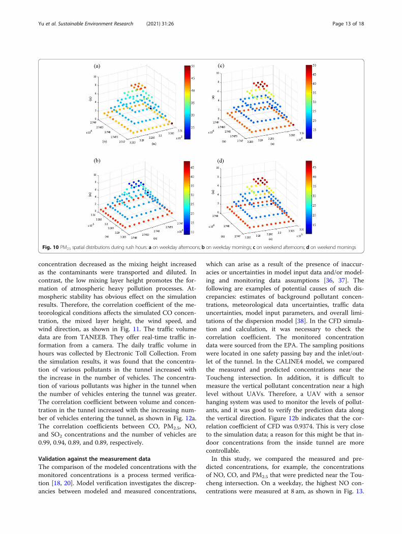
14 m), and the data for each hour were very close be-tween them. However, UAV monitoring was also af-fected by weather conditions.Figure 10 presents the concentration of PM2.5 with a

3D distribution. Generally, the concentration of PM2.5

decreased as the height increased, and the results weresimilar to those of another study [33]. Due to the min-imal ground emission source, no difference in all flightswas observed in the horizontal distribution. On weekdaymornings, the PM2.5 concentrations was approximately40–45 μg m− 3 at 1.5 m. The human activity caused theemissions of pollutants to accumulate [34, 35]. The ve-hicle volume on the highway during the week days waslower than that on weekends, and the concentration de-creased as the height increased. There is an incrementaltemperature in the air, while there is a rise in the solarenergy and radiation levels. Until the early afternoon,there was a gradual increase in the concentration of the

Fig. 7 Simulated hourly concentration of PM2.5 on the Toucheng highway intersection at (a) 9 m; b 7 m; c 5 m; and d 3 m. The x-axis and y-axisare Universal Transverse Mercator coordinate systems


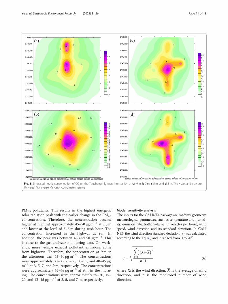
PM2.5 pollutants. This results in the highest energeticsolar radiation peak with the earlier change in the PM2.5

concentrations. Therefore, the concentration becamehigher at night at approximately 45–50 μg m− 3 at 1.5 mand lower at the level of 3–5 m during rush hour. Theconcentration increased in the highway at 9 m. Inaddition, the peak was between 48 and 50 μg m− 3. Thisis close to the gas analyzer monitoring data. On week-ends, more vehicle exhaust pollutant emissions comefrom highways. Therefore, the concentration at 9 m inthe afternoon was 45–50 μg m− 3. The concentrationswere approximately 30–35, 25–30, 30–35, and 40–45 μgm− 3 at 3, 5, 7, and 9 m, respectively. The concentrationswere approximately 45–48 μg m− 3 at 9 m in the morn-ing. The concentrations were approximately 25–30, 15–20, and 12–15 μg m− 3 at 3, 5, and 7 m, respectively.

Model sensitivity analysisThe inputs for the CALINE4 package are roadway geometry,meteorological parameters, such as temperature and humid-ity, emission rate, traffic volume (in vehicles per hour), windspeed, wind direction and its standard deviation. In CALINE4, the wind direction standard deviation (S) was calculatedaccording to the Eq. (6) and it ranged from 0 to 200.

S ¼

ffiffiffiffiffiffiffiffiffiffiffiffiffiffiffiffiffiffiffiffiffiffiffiffiffiXni¼1

Xi−X� �2n−1

vuuutð6Þ

where Xi is the wind direction, X is the average of winddirection, and n is the monitored number of winddirection.

Fig. 8 Simulated hourly concentration of CO on the Toucheng highway intersection at (a) 9 m; b 7 m; c 5 m; and d 3 m. The x-axis and y-ax areUniversal Transverse Mercator coordinate systems


The concentration rapidly dropped as the wind speedincreased, especially at 0.5–1m s− 1, and the CO concen-tration changed from 10 to 50 ppm. The wind directionstandard deviation is also important when the S is morethan 200. The CO concentration tended to be moderate,and the standard deviation of the wind direction was 50

at a CO concentration of approximately 120 ppb. The

standard deviation of wind direction was more than 200

when the concentration of CO remained at 50 ppb. At ahigh mixing layer height (1000 m), the concentration ofCO was 1.4–2.5 ppb. At a lower mixing layer height(500 m), the maximum CO concentration was approxi-mately 2.5–4.0 ppb. The contaminants were uniformlymixed by turbulence in the mixed layer since the

Fig. 9 a Hanging length with a sensor; b comparison of data from the UAV and EPA stations


concentration decreased as the mixing height increasedas the contaminants were transported and diluted. Incontrast, the low mixing layer height promotes the for-mation of atmospheric heavy pollution processes. At-mospheric stability has obvious effect on the simulationresults. Therefore, the correlation coefficient of the me-teorological conditions affects the simulated CO concen-tration, the mixed layer height, the wind speed, andwind direction, as shown in Fig. 11. The traffic volumedata are from TANEEB. They offer real-time traffic in-formation from a camera. The daily traffic volume inhours was collected by Electronic Toll Collection. Fromthe simulation results, it was found that the concentra-tion of various pollutants in the tunnel increased withthe increase in the number of vehicles. The concentra-tion of various pollutants was higher in the tunnel whenthe number of vehicles entering the tunnel was greater.The correlation coefficient between volume and concen-tration in the tunnel increased with the increasing num-ber of vehicles entering the tunnel, as shown in Fig. 12a.The correlation coefficients between CO, PM2.5, NO,and SO2 concentrations and the number of vehicles are0.99, 0.94, 0.89, and 0.89, respectively.

Validation against the measurement dataThe comparison of the modeled concentrations with themonitored concentrations is a process termed verifica-tion [18, 20]. Model verification investigates the discrep-ancies between modeled and measured concentrations,

which can arise as a result of the presence of inaccur-acies or uncertainties in model input data and/or model-ing and monitoring data assumptions [36, 37]. Thefollowing are examples of potential causes of such dis-crepancies: estimates of background pollutant concen-trations, meteorological data uncertainties, traffic datauncertainties, model input parameters, and overall limi-tations of the dispersion model [38]. In the CFD simula-tion and calculation, it was necessary to check thecorrelation coefficient. The monitored concentrationdata were sourced from the EPA. The sampling positionswere located in one safety passing bay and the inlet/out-let of the tunnel. In the CALINE4 model, we comparedthe measured and predicted concentrations near theToucheng intersection. In addition, it is difficult tomeasure the vertical pollutant concentration near a highlevel without UAVs. Therefore, a UAV with a sensorhanging system was used to monitor the levels of pollut-ants, and it was good to verify the prediction data alongthe vertical direction. Figure 12b indicates that the cor-relation coefficient of CFD was 0.9374. This is very closeto the simulation data; a reason for this might be that in-door concentrations from the inside tunnel are morecontrollable.In this study, we compared the measured and pre-

dicted concentrations, for example, the concentrationsof NO, CO, and PM2.5 that were predicted near the Tou-cheng intersection. On a weekday, the highest NO con-centrations were measured at 8 am, as shown in Fig. 13.

Fig. 10 PM2.5 spatial distributions during rush hours: a on weekday afternoons; b on weekday mornings; c on weekend afternoons; d on weekend mornings


Likewise, NO levels were higher on weekdays than onweekends, especially during the rush hour in the morn-ing. Provincial roads No. 2 and No. 9 are industrialroads, with trucks passing through this area to transportproducts. There are two peaks over the course of 24 h.The highest concentration is at 8 am. Additionally, theNO concentration was approximately 0.08 to 0.12 ppm.

The other peak is at 6 pm. Furthermore, the NO concen-tration was approximately 0.06 to 0.1 ppm. The simu-lated values correspond to the measured values, exceptin the afternoon. The difference in observed and simu-lated NO concentrations due to the terrain where thehighway is located in the valley. The trend is similar be-tween the observed and simulated NO concentrations

Fig. 11 a Relationship between wind speed and CO concentration; b the relationship between wind direction standard deviation and CO concentration


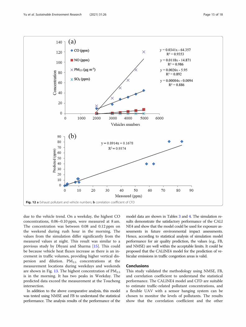
due to the vehicle trend. On a weekday, the highest COconcentrations, 0.06–0.10 ppm, were measured at 8 am.The concentration was between 0.08 and 0.12 ppm onthe weekend during rush hour in the morning. Thevalues from the simulation differ significantly from themeasured values at night. This result was similar to aprevious study by Dhyani and Sharma [15]. This couldbe because vehicle heat fluxes increase as there is an in-crement in traffic volumes, providing higher vertical dis-persion and dilution. PM2.5 concentrations at themeasurement locations during weekdays and weekendsare shown in Fig. 13. The highest concentration of PM2.5

is in the morning. It has two peaks in Weekday. Thepredicted data exceed the measurement at the Touchengintersection.In addition to the above comparative analysis, this model

was tested using NMSE and FB to understand the statisticalperformance. The analysis results of the performance of the

model data are shown in Tables 3 and 4. The simulation re-sults demonstrate the satisfactory performance of the CALINE4 and show that the model could be used for exposure as-sessments in future environmental impact assessments.Hence, according to statistical analysis of simulation modelperformance for air quality prediction, the values (e.g., FB,and NMSE) are well within the acceptable limits. It could beproposed that the CALINE4 model for the prediction of ve-hicular emissions in traffic congestion areas is valid.

ConclusionsThis study validated the methodology using NMSE, FB,and correlation coefficient to understand the statisticalperformance. The CALINE4 model and CFD are suitableto estimate traffic-related pollutant concentrations, anda flexible UAV with a sensor hanging system can bechosen to monitor the levels of pollutants. The resultsshow that the correlation coefficient and the other

Fig. 12 a Exhaust pollutant and vehicle numbers; b correlation coefficient of CFD


Fig. 13 Comparison of measured and predicted data: a NO on weekdays; b NO on weekends; c CO on weekdays; d CO on weekends; e PM2.5 onweekdays; f PM2.5 on weekends

Table 3 Statistical performance of the CALINE4

Statistical performanceindicators

NO CO PM2.5 NO CO PM2.5 Acceptablerange [14]Weekend Weekday

NMSE 0.4 0.09 0.08 0.2 0.2 0.09 NMSE ≤0.5

FB 0.1 0.09 −0.1 0.15 0.15 −0.1 − 0.5≤ FB ≤ 0.5

Correlation coefficient (r2) 0.66 0.50 0.51 0.74 0.67 0.50 r2 > 0.5


parameters are in a reasonable range, despite the trafficin this area being complicated. In the Hsuehshan tunnel,the vehicle speed is 40 km h− 1 when the fan is openedon the weekend, and SO2, CO, NO, and PM2.5 concen-trations are mainly distributed in the tunnel outlet, withconcentrations ranging from 0.001 to 0.004, 4.0 to 9.0,0.7 to 1.8 ppm, and 40 to 60 μg m− 3. On weekdays, SO2,CO, NO, and PM2.5 concentrations are mainly distrib-uted in the tunnel outlet, with concentrations rangingfrom 0.001 to 0.003, 2 to 6, 0.36 to 1.3, 0.36 to 1.08 ppm,and 20 to 55 μg m− 3. At the Toucheng Intersection, thesimulated PM2.5 concentrations located at 9.0, 7.0, 5.0,and 3.0 m were approximately 50 to 74 μg m− 3. On holi-days, the UAV monitoring concentrations were 40 to 45,25 to 30, 20 to 25, and 40 to 43 μg m− 3 in the morning.On the weekend, the highest pollutant emission ratecomes from Highway No. 5. The correlation coefficientsbetween traffic volume and CO, PM2.5, NO and SO2

concentrations were 0.99, 0.91, 0.89, and 0.89,respectively.The results provide information on vehicular exhaust

emissions in a long tunnel and along a 2 km length ofthe highway, including information on air quality to-gether with information on the three-dimensional spatialdistribution of PM2.5 concentrations. These data are use-ful for transportation planners working towards a trafficmanagement plan. Meanwhile, this study provides a ref-erence method to be used for environmental impact as-sessments for long tunnels and areas prone to trafficjams. For future research, CFD could simulate volatileorganic compounds in indoor environments to evaluatethe relationships between volatile organic compound useand health. Compared with the traditional measurementpollutant concentration method, UAVs with sensorhanging systems have many advantages in measuringvertical pollutants, thus they address the limitations offuture studies.

AcknowledgementsThe authors wish to thank the students of Air Pollution Control Laboratory,National Ilan University for their assistance in monitoring and sampling.

Authors’ contributionsShin Yu conceptualized the study, conducted laboratory works, provided thestatistics, processed the data and fulfilled the analysis, wrote the draft. ChangTang Chang provided software and performed the analysis supervision, draftwriting supervision. Chih Ming Ma performed the analysis supervision, finalmanuscript writing and editing. All authors read and approved the finalmanuscript.

FundingThis work was supported by Grant MOST105–2221-E-562-002-MY3.

Availability of data and materialsAll data generated or analyzed during this study are available upon request.

Declaration

Competing interestsThe authors declare they have no competing interests.

Author details1Department of Environmental Engineering, National Ilan University, Yilan260007, Taiwan. 2Department of Cosmetic Application and Management, St.Mary’s Junior College of Medicine, Nursing and Management, SanxingTownship 266003, Taiwan.

Received: 31 January 2021 Accepted: 12 July 2021

References1. Chuang HC, Ho KF, Lin LY, Chang TY, Hong GB, Ma CM, et al. Long-term

indoor air conditioner filtration and cardiovascular health: a randomizedcrossover intervention study. Environ Int. 2017;106:91–6.

2. Carslaw DC, Priestman M, Williams ML, Stewart GB, Beevers SD. Performanceof optimised SCR retrofit buses under urban driving and controlledconditions. Atmos Environ. 2015;105:70–7.

3. Saini J, Dutta M, Marques G. A comprehensive review on indoor air qualitymonitoring systems for enhanced public health. Sustain Environ Res. 2020;30:6.

4. Chuang KJ, Lin LY, Ho KF, Su CT. Traffic-related PM2.5 exposure and itscardiovascular effects among healthy commuters in Taipei, Taiwan. AtmosEnviron-X. 2020;7:100084.

5. Chen RY, Ho KF, Hong GB, Chuang KJ. Houseplant, indoor air pollution, andcardiovascular effects among elderly subjects in Taipei, Taiwan. Sci TotalEnviron. 2020;705:135770.

6. Polidori A, Arhami M, Sioutas C, Delfino RJ, Allen R. Indoor/outdoorrelationships, trends, and carbonaceous content of fine particulate matter inretirement homes of the Los Angeles basin. J Air Waste Manage. 2007;57:366–79.

7. Kaur S, Nieuwenhuijsen MJ, Colvile RN. Fine particulate matter and carbonmonoxide exposure concentrations in urban street transportmicroenvironments. Atmos Environ. 2007;41:4781–810.

8. Fruin S, Westerdahl D, Sax T, Sioutas C, Fine PM. Measurements andpredictors of on-road ultrafine particle concentrations and associatedpollutants in Los Angeles. Atmos Environ. 2008;42:207–19.

9. Huertas JI, Prato DF. CFD modeling of near-roadway air pollution. EnvironModel Assess. 2020;25:129–45.

10. Okokon EO, Yli-Tuomi T, Turunen AW, Taimisto P, Pennanen A, Vouitsis I,et al. Particulates and noise exposure during bicycle, bus and carcommuting: a study in three European cities. Environ Res. 2017;154:181–9.

11. Campagnolo D, Cattaneo A, Corbella L, Borghi F, Del Buono L, Rovelli S,et al. In-vehicle airborne fine and ultra-fine particulate matter exposure: theimpact of leading vehicle emissions. Environ Int. 2019;123:407–16.

12. Barnes MJ, Brade TK, MacKenzie AR, Whyatt JD, Carruthers DJ, Stocker J,et al. Spatially-varying surface roughness and ground-level air quality in anoperational dispersion model. Environ Pollut. 2014;185:44–51.

13. Batterman SA, Zhang K, Kononowech R. Prediction and analysis of near-road concentrations using a reduced-form emission/dispersion model.Environ Health-Glob. 2010;9:29.

14. Dhyani R, Singh A, Sharma N, Gulia S. Performance evaluation of CALINE 4model in a hilly terrain – a case study of highway corridors in HimachalPradesh (India). Int J Environ Pollut. 2013;52:244–62.

15. Dhyani R, Sharma N. Sensitivity analysis of CALINE4 model under mix trafficconditions. Aerosol Air Qual Res. 2017;17:314–29.

16. Baik JJ, Kim JJ, Fernando HJS. A CFD model for simulating urban flow anddispersion. J Appl Meteorol Clim. 2003;42:1636–48.

17. Tominaga Y, Stathopoulos T. Turbulent Schmidt numbers for CFD analysiswith various types of flowfield. Atmos Environ. 2007;41:8091–9.

Table 4 Performance evaluation of CALINE4 model

NMSE FB

This study 0.09–0.4 −0.1–0.2

Dhyani et al. [14] 0.05–1.8 −1.2–0.2

Dhyani and Sharma [15] 0.09 0.3


18. Wang XF, Conboy K, Cawley O. "Leagile" software development: anexperience report analysis of the application of lean approaches in agilesoftware development. J Syst Software. 2012;85:1287–99.

19. Qin DC, Guo B, Zhou J, Cheng HM, Chen XK. Indoor air formaldehyde(HCHO) pollution of urban coach cabins. Sci Rep-UK. 2020;10:332.

20. Cardozo JIH, Sanchez DFP. An experimental and numerical study of airpollution near unpaved roads. Air Qual Atmos Hlth. 2019;12:471–89.

21. Santiago JL, Martilli A, Martin F. CFD simulation of airflow over a regulararray of cubes. Part I: three-dimensional simulation of the flow andvalidation with wind-tunnel measurements. Bound-Lay Meteorol. 2007;122:609–34.

22. Llaguno-Munitxa M, Bou-Zeid E, Hultmark M. The influence of buildinggeometry on street canyon air flow: validation of large eddy simulationsagainst wind tunnel experiments. J Wind Eng Ind Aerod. 2017;165:115–30.

23. Bari S, Naser J. Simulation of airflow and pollution levels caused by severetraffic jam in a road tunnel. Tunn Undergr Sp Tech. 2010;25:70–7.

24. Bhautmage U, Gokhale S. Effects of moving-vehicle wakes on pollutantdispersion inside a highway road tunnel. Environ Pollut. 2016;218:783–93.

25. Zhang CH, Kovacs JM. The application of small unmanned aerial systems forprecision agriculture: a review. Precis Agric. 2012;13:693–712.

26. Hien VTD, Lin C, Thanh VC, Oanh NTK, Thanh BX, Weng CE, et al. Anoverview of the development of vertical sampling technologies for ambientvolatile organic compounds (VOCs). J Environ Manage. 2019;247:401–12.

27. Hildmann H, Kovacs E. Review: Using unmanned aerial vehicles (UAVs) asmobile sensing platforms (MSPs) for disaster response, civil security andpublic safety. Drones. 2019;3:59.

28. Gu QJ, Michanowicz DR, Jia CR. Developing a modular unmanned aerialvehicle (UAV) platform for air pollution profiling. Sensors-Basel. 2018;18:4363.

29. Ma CM, Hong GB, Chang CT. Influence of traffic flow patterns on air qualityinside the longest tunnel in Asia. Aerosol Air Qual Res. 2011;11:44–50.

30. Thompson JF, Soni BK, Weatherill NP, editors. Handbook of grid generation.1st Boca Raton: CRC Press; 1998.

31. Rhys-Tyler GA, Legassick W, Bell MC. The significance of vehicle emissionsstandards for levels of exhaust pollution from light vehicles in an urbanarea. Atmos Environ. 2011;45:3286–93.

32. Burr ML, Karani G, Davies B, Holmes BA, Williams KL. Effects on respiratoryhealth of a reduction in air pollution from vehicle exhaust emissions. OccupEnviron Med. 2004;61:212–8.

33. Peng ZR, Wang DS, Wang ZY, Gao Y, Lu SJ. A study of vertical distributionpatterns of PM2.5 concentrations based on ambient monitoring withunmanned aerial vehicles: a case in Hangzhou, China. Atmos Environ. 2015;123:357–69.

34. Cheng YH, Liu ZS, Chen CC. On-road measurements of ultrafine particleconcentration profiles and their size distributions inside the longesthighway tunnel in Southeast Asia. Atmos Environ. 2010;44:763–72.

35. He LY, Hu M, Zhang YH, Huang XF, Yao TT. Fine particle emissions from on-road vehicles in the Zhujiang Tunnel, China. Environ Sci Technol. 2008;42:4461–6.

36. Kastner-Klein P, Plate EJ. Wind-tunnel study of concentration fields in streetcanyons. Atmos Environ. 1999;33:3973–9.

37. Sagrado APG, van Beeck J, Rambaud P, Olivari D. Numerical andexperimental modelling of pollutant dispersion in a street canyon. J WindEng Ind Aerod. 2002;90:321–39.

38. El-Harbawi M. Air quality modelling, simulation, and computationalmethods: a review. Environ Rev. 2013;21:149–79.

Publisher’s NoteSpringer Nature remains neutral with regard to jurisdictional claims inpublished maps and institutional affiliations.


simulation and measurement of air quality in the traffic

Documents