Simulation and Verification of Laminar Pipe Flows

57:020 Intermediate Mechanics of Fluids CFD PRELAB 1

By Tao Xing and Fred Stern

1. Purpose The Purpose of CFD PreLab 1 is to teach students how to use the CFD educational interface (FlowLab 1.2), be familiar with the options in each step of CFD Process, and relate simulation results to AFD concepts. Students will simulate laminar pipe flow following “CFD process” by an interactive step-by-step approach. Students will have “hands-on” experiences using FlowLab to compute axial velocity profile, centerline velocity, and friction factor on three different meshes (Verification). Students will compare simulation results with AFD data, analyze the differences and possible numerical errors, and present results in Lab report.

Geometry parameters

Select Geometry

Geometry

IniCond

BounCond

Compibl

HeTran

FloProp

ViscMo

Solve t

Flow Chart f

2. Simulation

Physics

Own geom

Nozzl

e

St

U

tial itions

dary itions

ress-e?

at sfer?

w erties

Densi

Lamin

Turbu

Invisc

ous dels

or ISTUE T

Design

Mesh

etry

e

Coarse

Medium

Automatic

Manualructured

nstruct-ured

One Eq.

Two Eq.

ty and viscosity

ar

len

id

SA

k-w

k-e

Fine

Total pressure drop

XY plot

Validation

Verification

Iterations/ Steps

Converge-nt

LimitPrecisions Single

DoubleNumerical Schemes

Steady/ Unsteady?

Quick

2nd order upwind

1st order upwind

eaching Module for Pipe flow (red color illustrates the o

use in this CFD PreLab 1)

Post-processing

Wall friction

Streamlines

Vectors

Contours

Centerline Velocity

Centerline Pressure

Profiles of Axial Velocity

Pip

Sudden Expansion

Diffuser

Repor

ptions you will

1

In EFD Lab 2, you have conducted experimental study for turbulent pipe flow. The data you have measured will be used for CFD Lab 1. In CFD PreLab 1, simulation will be conducted only for laminar pipe flows, i.e. the inlet velocity (or Reynolds number) will be less than that for turbulent pipe flows. Comparisons between CFD and AFD can be conducted. The problem to be solved is that of laminar/turbulent flows through a circular pipe. Reynolds number is 655 for laminar pipe flow, based on pipe diameter.

Since the flow is axisymmetric we only need to solve the flow in a single plane from the centerline to the pipe wall. Boundary conditions need to be specified for inlet, outlet, wall, and axis, as described later. Uniform flow was specified at inlet, the flow will reach the fully developed regions after a certain distance downstream. No-slip boundary condition will be used for the wall and constant pressure for outlet. Symmetric boundary condition will be applied on the axis. Since the flow is laminar, turbulence models are not necessary. Analytical solutions (AFD) for Laminar Pipe Flow will be provided by TA of this Lab. 3. CFD Process Step 1: (Geometry)

1. Radius of pipe (0.02619 m) 2. Length of pipe (7.62 m)

Click <<Create>>, after you see the pipe geometry created, click <<Next>>. Step 2: (Physics)

OutletInlet Symmetry Axis

Pipe Wall

2

1. With or without Heat Transfer? Since we are dealing only with the flow and not with the thermal aspects of the flow like heat transfer etc, switch the <<heat transfer >> button off, which is the default setup. 2. Incompressible or compressible Choose “Incompressible”, which is the default setup. 3. Flow Properties

use the values shown in the above figure. Input the values and click <<OK>> 4. Viscous Model

In CFD PreLab 1, Choose laminar model and click <<OK>>.

3

5. Boundary Conditions At “Inlet”, we use zero gradient for pressure and fix the velocity to be 0.2m/s.

At “Axis”, FlowLab use zero gradient for axial velocity and Pressure and specify the magnitude for radial velocity to be zero. Read all the values and click <<OK>>

At “Outlet”, FlowLab uses magnitude for pressure and zero gradients for axial and radial velocities. Input “0” for the Gauge pressure and click <<OK>>

At “Wall”, no-slip boundary conditions are fixed for both axial and radial velocity, gradient for pressure is zero. Read the panel and click <<OK>>

6. Initial Conditions Use the following setup for initial conditions.

4

After specifying all the above parameters, click <<compute>> button and FlowLab will automatically calculate the Reynolds number based on the inlet velocity and pipe diameter you input. Click the <<next>>, this takes you to the next step, “Mesh”. Step 3: (Mesh)

For CFD PreLab 1, “Structured” meshes will be generated using either “Automatic” or “Manual” generations (see exercises at the end of this document for details). NR and NX is the number of intervals in axial and radial directions. For “Automatic” generation, just choose the mesh density: “coarse”, “medium” or “fine”, and click <<Create>>, FlowLab will automatically create the mesh you required and display the grid information NR, NX. For manually generation, you should first choose the “Manual” button, and then the following panel will be shown:

5

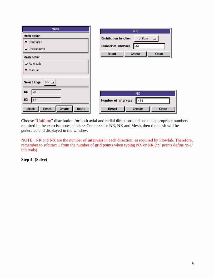
Choose “Uniform” distribution for both axial and radial directions and use the appropriate numbers required in the exercise notes, click <<Create>> for NR, NX and Mesh, then the mesh will be generated and displayed in the window. NOTE.: NR and NX are the number of intervals in each direction, as required by Flowlab. Therefore, remember to subtract 1 from the number of grid points when typing NX or NR (‘n’ points define ‘n-1’ intervals) Step 4: (Solve)

6

The flow is steady, so turn on the “Steady” option and turn off the “Unsteady” option. Specify the iteration number and convergence limit to be 10000 and 10-6 respectively. Use 10, 20, 40, 60, 100 for radial profile x/D positions and choose “Double precision” with “2nd order upwind scheme”. Use “New” calculation for this Lab. Then click <<iterate>> and FlowLab will begin the calculation, whenever you see the window, “Solution Converged”. Click <<OK>>.

The iterative history of residuals for continuity equation and X and Y momentum equations will be shown automatically. (NOTE: By now, you have to hit the XY plot tab in the menu bar twice (at bottom of screen) to bring up the Residual Plot window to the front and view residual behavior when you are running the exercises, similar to other XY plots).

7

Step 5: (Reports) Plot the XY plot for “wall friction factor distribution” and record the “wall friction factor” in the developed region (near outlet) and compare its value with the AFD data. Import AFD data for axial velocity profile and compare with CFD predictions in the XY plot.

8

“XY Plots” provide options to plot axial velocity profile (axial velocity vs. radial locations), centerline pressure/velocity distribution (pressure/velocity vs. x). The following figure shows the example for axial velocity profile:

To import the AFD data and put on top of the above CFD results, just click <<File>> button and use the browse button to locate the file you want and click <<Import>>.

9

You can also click <<Curves>> to choose which curve will be displayed, use “Ctrl” and left button of the mouse for multiple choices. To save the figure, click <<hardcopy>>. In this Lab:

1. AFD data for developed laminar axial velocity profile is at: C:\Documents and Settings\Fluidslab\myflowlab\axialvelocityAFD.xy

Verification and Validation In CFD PreLab 1, you will also conduct verification studies using the manually mesh generation options. (read exercise notes for details). The V&V panel is shown below. Whenever you manually create a mesh, that mesh will be automatically used as the default “fine” mesh for verification.

10

11

First input the refinement ratio you will use for the “coarse”, “medium”, and “fine” meshes. “Monitor location” is used to specify the locations for line monitors (verification of axial velocity profile) and will NOT be used in this PreLab.

Click <<Run>>, FlowLab will conduct simulation in the order of “fine mesh” “medium mesh” “coarse mesh”. The information on which mesh is solving now will be displayed in the left bottom window.

After all three meshes solved, you can click “Show Outlet Velocity”, then outlet velocity on three meshes will be shown together, import AFD data and tell which mesh predictions of axial velocity profile is the closest to AFD data.

You can also select which variables you want to be shown for verification results. In this Lab, you choose “friction factor”. Click “show verification”, you will get two tables: verification results table and the errors table. You need save both using “Alt+printScreen” and paste into WORD document. The following figures are samples.

Step 6: (Post-processing)

To show pressure contour, choose “contour”, click <<Activate>>, contour for axial velocity will be shown. You can then click <<Modify>> button to select different variables if you need. For a better view, press and hold the right button of the mouse and drag towards you, you will have a figure similar to the following:

NOTE: If you happen to rotate the figure, such as the following:

12

You can always use the button to align the pipe with the coordinate and use to view the full size of the pipe. To view velocity vectors, click <<Close>> on the modify panel, and select <<vector>> with <<Activate>>, if you don’t want pressure contour you plotted before to be shown, just choose <<contour>> and then click <<Deactivate>>. The following showing an example for velocity vectors example.

Note that, you can press and hold the middle button of the mouse and move to left or right to choose the intersection while the flow begins to become fully developed flows. Just as shown above. You can also use the <<Edit>> button for vectors to specify the better “scale” value.

13

14

Exercises You need finish the following assignments and present results in your lab reports following the lab report instructions

Simulation and Verification Study of Laminar Pipe Flow * You must save each case file for each exercise using “file” “save as”

1. Compare CFD with AFD on friction factor: Use “automatic” “medium” mesh, and all other default values in the instructions, iterate the simulation until it converges. Find the relative error between AFD friction factor(0.097747231) and CFD. Note: (1). Figures need to be saved: residual history, centerline pressure, centerline velocity, wall friction factor, contour of axial velocity, and velocity vectors. (2). Data need to saved: friction factor in the developed region, developing length.

NOTE: (1). To easily get the friction factor, you can plot “XY plot” under “Reports” first, click <<file>>button and then export file to the name you want. Use Excel to open that file and use the value closest to pipe outlet.

2. Verification for friction factor: use 2nd order upwind scheme with “ UlaminarU” model,

“ Udouble precisionU” and create UuniformU meshes using “UmanualU” function. Manually generate a mesh with 452 grid points in axial direction (X) and 45 points in the radial direction (R) (mesh 3). This mesh will be used as the “fine” mesh in verification study. Use convergent limits 10P

-6P and run verification using grid refinement ratio 1.414.

Meshes Pg Cg Ug(%) Ugc (%)

1,2,3

NOTE: (1). You only need create mesh 3 manually, when you click “run” in verification, FlowLab will automatically create the “medium” (mesh 2) and “coarse” mesh (mesh 1) (2). X and R should be NX+1 and NR+1 since NX and NR are the number of intervals. So, when you can create mesh manually, you need use NX, NR (451×44) for mesh 3. (3). Don’t specify any line monitor locations. (4). Figure need to be saved: residuals history for mesh 3, FlowLab “Errors” panel and “Verification” panel for friction factor. (5). Data need to be saved: the above table with values.

3. Questions need to be answered when writing CFD Lab 1 report:

3.1. Bind your answers to CFD PreLab1 questions with your CFD Lab 1 report 3.2. Answer all the questions in exercises 1 to 2 3.3. Analyze the difference between CFD and AFD and possible error sources. 3.4. Summarize your findings by analyzing the results (contours, centerline velocity distributions, centerline pressure distributions, etc.) and relate those findings to your classroom lectures or textbooks.

15