simulation-based optimization of football defenses
TRANSCRIPT

Simulation-Based Optimization
of Football Defenses
Daman Oberoi
Alan Fern
Department of Electrical Engineering and Computer Science
Oregon State University
December 7, 2006

1
Abstract
We develop a system for simulation-based optimization of defensive formations for
American football. The first component of the system is an environment for simulating football
plays with real physical interactions between players and their surroundings. The simulator is
built on the AGEIA PhysX engine, which incorporates rigid body dynamics and collision
detection. The simulator allows a user to design, visualize, and execute distinct plays for each
offensive player. In addition, the camera angle and zoom can be adjusted to suit the user's needs.
The second component of the system is a genetic algorithm that uses the simulator to optimize
the defensive formation based on the offense's playbook and its likelihood of running each play.
We show that this technique effectively tunes defenses to a variety of game situations.

2
Table of Contents
Abstract .......................................................................................................................................... 1
List of Figures ................................................................................................................................ 3
List of Tables ................................................................................................................................. 4
1 Introduction ............................................................................................................................ 5
2 A Simulator for American Football ...................................................................................... 5
2.1 Simulator Infrastructure................................................................................................. 5
2.2 Description of Football Environment ............................................................................ 6
2.3 Implementation ................................................................................................................ 6
3 Optimizing Football Defenses .............................................................................................. 10
3.1 Problem Description ....................................................................................................... 10
3.2 GA Background ............................................................................................................. 11
3.3 Applying a Genetic Algorithm to Football .................................................................. 12
4 Experiments........................................................................................................................... 14
4.1 Player Attributes ............................................................................................................ 14
4.2 Experimental Results..................................................................................................... 15
5 Summary and Future Work ................................................................................................ 25
Appendix A: Player Routes ........................................................................................................ 28
Appendix B: Probability Distributions ..................................................................................... 33
Appendix C: Fitness Graphs ...................................................................................................... 34
Appendix D: Defensive Performances After 50 Generations ................................................. 45
Appendix E: Comparison of Distribution Rankings ............................................................... 49
Appendix F: Simulator Instructions ......................................................................................... 53

3
List of Figures
Figure 1: Allowed player directional movements.......................................................................... 7
Figure 2: Offensive player routes .................................................................................................. 8
Figure 3: Example of a chromosome, genes, and alleles ............................................................. 11
Figure 4: Best fitness per generation for Defense A .................................................................... 23
Figure 5: Population fitness per generation for Defense A ......................................................... 24
4
List of Tables
Table 1: Probability Distribution A ............................................................................................. 13
Table 2: Player attributes by position. ......................................................................................... 14
Table 3: Defensive performances on Distribution A. .................................................................. 16
Table 4: Defensive performances on Distribution B. .................................................................. 16
Table 5: Raw results of Defenses A and B. ................................................................................. 16
Table 6: Defensive performances on Distribution C. .................................................................. 17
Table 7: Defensive performances on Distribution D. .................................................................. 18
Table 8: Raw results of Defenses C and D. ................................................................................. 18
Table 9: Defensive performances on Distribution E. ................................................................... 19
Table 10: Raw results of Defense E. ............................................................................................ 19
Table 11: Defensive performances on Distribution F. ................................................................. 20
Table 12: Defensive performances on Distribution G. ................................................................ 20
Table 13: Raw results of Defenses F and G. ................................................................................ 20
Table 14: Defensive performances on Distribution H. ................................................................ 21
Table 15: Defensive performances on Distribution I. .................................................................. 21
Table 16: Raw results of Defenses H and I. ................................................................................. 22
Table 17: Defensive performances on Distribution J................................................................... 22
Table 18: Raw results of Defense J. ............................................................................................. 22
Table 19: Raw results of Defenses B and I. ................................................................................. 25

5
1 Introduction
Imagine you are the coach of a football team in a hotly contested game. Your defense is
on the field and the game is on the line. Your team must get a defensive stop on the next series of
plays in order to have any chance of winning this game. Which plays do you call? Suppose you
have reviewed extensive tape on your opponent and are pretty confident about the distribution of
plays they will execute. You instruct your defense to set up accordingly, and on the next play
your players tackle the running back for a two yard loss. Congratulations.
This is precisely the type of scenario that our work aims to handle. This paper describes
how this project takes a first step in that direction. We develop a 3D simulator for American
football where the players interact with their environment based on real physics. Each offensive
player is dictated a distinct route, and the defense’s goal is to minimize the offense’s gain. We
employ a genetic algorithm to optimize the location of each defender. By running simulations
repeatedly, the genetic algorithm should strategically place defenders and allow them to
significantly curtail the number of yards gained by the offense.
Before continuing, we would like to distinguish between the terms location and position
as they are used throughout this paper. The former is used in reference to the placement of an
object in the environment. The latter is used to refer to the type of player (quarterback, running
back, safety, etc.) in the football domain.
Section 2 explains the game of football and elaborates on the infrastructure and
implementation of the simulator. Section 3 describes the problem we are solving, introduces
genetic algorithms, and illustrates how to apply a genetic algorithm to the problem at hand.
Section 4 discusses the experimental design and results. Finally, section 5 provides a summary
and suggests future work.
2 A Simulator for American Football
2.1 Simulator Infrastructure
The foundation of the simulator is comprised of the AGEIA PhysX engine, OpenGL, and
the OpenGL Utility Toolkit, better known as GLUT. AGEIA PhysX is touted as the world’s first
dedicated physics engine that allows for unscripted physical reality. It unites rigid body
dynamics simulation and collision detection into one package [1]. In our work, PhysX is used to
build the arena, draw all players, and run the simulation with realistic interactions between
players and the environment. OpenGL is a popular 2D and 3D graphics application programming
interface (API) that can be ported across all systems [2]. Since OpenGL is system independent, a
library of utilities called GLUT exists for OpenGL on each system [3]. We use OpenGL and
GLUT to accept user input, draw the viewing window and its contents, and control the camera,
lighting, and colors.

6
2.2 Description of Football Environment
Football is an extremely popular sport in American culture. It is played on a rectangular
field 100 yards in length with end zones and goal posts at each end. There are 11 players for each
of two teams on the field at any given time. The primary goal is to obtain possession of the ball
and advance it through a series of running and passing plays into the opponent’s end zone. The
offense gets four chances, or downs, to advance the ball, starting at the line of scrimmage. If the
offense gains at least 10 yards beyond the line of scrimmage, it is awarded another 4 downs.
Upon entering the end zone with the ball, a team scores a touchdown worth six points, and then
has the opportunity to kick the ball through the goal posts for an additional point [4]. Football
has more rules and scoring options than described here, but this provides the essence of the
game.
In building the simulator, it is essential that it incorporate and simulate fundamental
aspects of the game of football. First, the simulator should allow for three-dimensional shapes
and at least two-dimensional motion; the availability of a third dimension of motion is preferable
in the event that the experiments should require that in the future. Secondly, the simulator must
include 11 players from each team and allow them to act independently and simultaneously. It is
important that we be able to control the size of each player and their starting locations and
movements on the field. Thirdly, we need to build a suitable stadium. Specifically, this includes
a playing field and walls along the out of bounds lines. While no such walls exist along a real
football field, we prefer that players bounce off walls and remain in play rather than running out
of bounds. In fact, we require that players interact with everything in their environment, namely
the ground, walls, and other players, based on real physics. On a related note, we need to
identify when a defensive player comes into contact with the offensive player who has the ball in
order to declare the play dead at that point. Finally, we need to rerun the simulation
automatically based on two events: (1) the offense has been tackled, or (2) the offense scores a
touchdown.
While the critical requirements of the simulator have been described above, there are
several other features that would prove helpful. With 22 players on the field, it could be very
difficult to identify the role of each one. Consequently, it would be nice if players could be
colored independently. Furthermore, being able to select a player and get more information about
him, such has his field coordinates and position, would likely be quite useful. Also, the ability to
control the camera angle and zoom would be a nice feature. Lastly, we would like to be able to
control the speed of the simulation.
2.3 Implementation
The essence of the simulator is the AGEIA PhysX engine, which includes a 3D
environment where arbitrary shapes can be defined and can interact with their environment based
on physical reality. OpenGL allows us to set the initial camera properties and control the color of
individual objects and the lighting on the scene. By monitoring input from the keyboard and
mouse, GLUT allows us to interactively change the camera angle and zoom, select a player on
the field, and specify which offensive routes to draw.

7
Although OpenGL can draw arbitrary polygons, we use the drawing functionality of
PhysX in order to allow players to interact with the environment. Specifically, the players are
represented as spheres, two units in diameter. The stadium consists of a green ground plane and
four walls. Technically, the ground plane is infinite in size, but the walls limit the size of the
stadium. PhysX has parameters for both static friction and dynamic friction. Static friction is the
force that acts when there is no relative motion between two objects, in this case, a player and the
ground. Dynamic friction is the resistance between two objects in contact, of which at least one
is in motion [5]. In this simulator, both types of friction have been set to zero. This allows for
freer motion of the players and results in a smoother simulation. Also, the coefficient of
restitution, which controls the amount of bouncing between objects, particularly between two
players in our experiment, has been set to just 0.05 to minimize excessive bouncing.
The PhysX environment has a left-handed coordinate system, so all objects have a
specific three-dimensional coordinate location. This makes it simple to specify the placement of
each object in the scene. Dynamic objects can move about the scene by applying a force or
specifying a velocity. In our simulator, all players move with a constant speed dependent on their
position. At each time step, every player can move in only one of eight directions: straight up,
diagonal up-right, straight right, diagonal down-right, straight down, diagonal down-left, straight
left, and diagonal up-left. See Figure 1. Each dynamic object has its own thread and, therefore,
all objects update simultaneously at each time step.
Figure 1: The eight directions a player can move at each time step.
Each offensive player is given a specific route to run on each play. The route is indicated
by a set of five waypoints. At each time step, the player chooses the direction closest to the
straight line between his current location and the waypoint destination. Essentially, there is no
guarantee that a player will reach his destination exactly. Instead, he reaches the waypoint
approximately by making the best decision on a heading at each time step. In order to prevent a
player from toggling back and forth near a waypoint, we require that a player pass through at
least one of the x or z coordinates of the waypoint and then continue towards the next waypoint.
See Figure 2 for examples of player routes.

8
Figure 2: Shown are the routes of the offensive players. The running back is red for easy
identification. The running back’s route is shown in red, with each of the five waypoints
indicated by black circles. The routes of the other offensive players are shown in yellow with the
waypoints in red. Fewer than five waypoints can be seen for some players because their
waypoints are repeated, effectively shortening their route. The defense has been excluded from
this screenshot for clarity.
This project focuses on only offensive rushing plays; we have not implemented the
capability to handle passing. As a result, the simulator uses only players as dynamic objects; no
ball exists. While the design of a play may make it look like the ball is hiked and handed off
from the quarterback to the running back, in reality the running back is assumed to have the ball
at all times. A play is terminated when the running back reaches the end zone or when he comes
into contact with a defensive player. In either case, the next play begins automatically with the
offense starting at the same location on each iteration. We do not simulate advancement of the
offense on each play as in a real football game.
If an offensive player completes his route before the play is over, the player will continue
in a straight line downfield towards the end zone (downward in Figure 2). The quarterback is the
only exception to this rule; he does not move in any pre-determined direction after completing
his route. As the offensive player moves downfield, he looks to block the closest defensive

9
player within a pre-specified radius called a zone. We specify this zone radius dependent on each
player’s position. Although the quarterback does not run downfield, he does block defensive
players that enter his zone. The running back also runs downfield after completing his route, but
he does not block any defensive players. The running back is not intelligent enough to avoid
defensive players; he runs in a straight line regardless of who is in his path. Sometimes, however,
a group of offensive players obstruct his straight-line path towards the end zone. In such a
scenario, the running back bounces off his own players and may find another straight-line path
that leads to the end zone.
The defense has a much simpler strategy: everyone plays zone defense. A defensive
player only moves when an offensive player enters his zone radius. The ultimate goal of the
defense is to tackle the running back, who is the only player to ever possess the imaginary ball.
However, the defense never has any knowledge of the running back or his location. Therefore, a
defender attacks the nearest offensive player in his zone radius with the hope that he might be the
running back. Effectively, the defense stops the running back in one of three ways:
1) A defender is located where he does not get blocked and the running back runs closely
enough for the defender to pursue and touch the running back,
2) A offensive blocker pushes the defensive player into the running back,
3) A collection of defenders jam the path of the running back to the point where the blockers
cannot push them out, and the running back has no choice but to get tackled.
Surprisingly, one of the greatest challenges in building the simulator is controlling the
timing and speed of the simulation. The PhysX engine has a built-in clock, and the simulation
slows as more objects are added to the scene. Given the number of iterations that have to run for
this project, it is absolutely necessary to increase the pace of the simulations. The timing is
controlled predominantly by two functions: setTiming() and simulate(). The latter function
expects a real number, elapsedTime, as an input parameter and advances the simulation by that
amount of time. If elapsedTime is large, it is internally subdivided according to the parameters
passed to the function setTiming(). The setTiming() function takes three input parameters:
- NxReal maxTimestep: The default value is 1.0f / 60.0f.
- NxU32 maxIter: The default value is 8.
- NxTimeStepMethod method: The default value is NX_TIMESTEP_FIXED.
If method is NX_TIMESTEP_FIXED, elapsedTime is internally subdivided into at most maxIter
sub-steps that are no larger than maxTimestep. If elapsedTime is not a multiple of maxTimestep,
any remaining time is added to elapsedTime for the next time step. If more sub-steps than
maxIter are required to advance the simulation by elapsedTime, the remaining time is
accumulated for the next call to simulate(). Although other values can be used for method,
NX_TIMESTEP_FIXED is strongly recommended for a stable, reproducible simulation [1].
We experimented with several values for the timing. The goal was to find a setting that
would increase the rate of the simulation, but still be slow enough to allow for visual inspection
of each play. This was important as we were still determining a variety of experimental
10
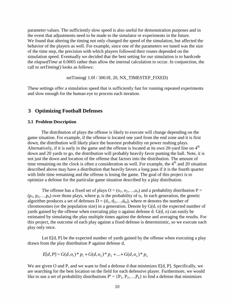
parameter values. The sufficiently slow speed is also useful for demonstration purposes and in
the event that adjustments need to be made to the simulator or experiments in the future.
We found that altering the timing not only changed the speed of the simulation, but affected the
behavior of the players as well. For example, since one of the parameters we tuned was the size
of the time step, the precision with which players followed their routes depended on the
simulation speed. Eventually we decided that the best setting for our simulation is to hardcode
the elapsedTime at 0.0005 rather than allow the internal calculation to occur. In conjunction, the
call to setTiming() looks as follows:
setTiming( 1.0f / 300.0f, 20, NX_TIMESTEP_FIXED)
These settings offer a simulation speed that is sufficiently fast for running repeated experiments
and slow enough for the human eye to process each iteration.
3 Optimizing Football Defenses
3.1 Problem Description
The distribution of plays the offense is likely to execute will change depending on the
game situation. For example, if the offense is located one yard from the end zone and it is first
down, the distribution will likely place the heaviest probability on power rushing plays.
Alternatively, if it is early in the game and the offense is located at its own 20-yard line on 4th
down and 20 yards to go, the distribution will probably heavily favor punting the ball. Note, it is
not just the down and location of the offense that factors into the distribution. The amount of
time remaining on the clock is often a consideration as well. For example, the 4th
and 20 situation
described above may have a distribution that heavily favors a long pass if it is the fourth quarter
with little time remaining and the offense is losing the game. The goal of this project is to
optimize a defense for the particular game situation described by a play distribution.
The offense has a fixed set of plays O = (o1, o2,…,on) and a probability distribution P =
(p1, p2,…,pn) over those plays, where pi is the probability of oi. In each generation, the genetic
algorithm produces a set of defenses D = (d1, d2,…,dm), where m denotes the number of
chromosomes (or the population size) in a generation. Denote by G(d, o) the expected number of
yards gained by the offense when executing play o against defense d. G(d, o) can easily be
estimated by simulating the play multiple times against the defense and averaging the results. For
this project, the outcome of each play against a fixed defense is deterministic, so we execute each
play only once.
Let E[d, P] be the expected number of yards gained by the offense when executing a play
drawn from the play distribution P against defense d.
nn podGpodGpodGPdE *),(...*),(*),(],[ 2211
We are given O and P, and we want to find a defense d that minimizes E[d, P]. Specifically, we
are searching for the best location on the field for each defensive player. Furthermore, we would
like to use a set of probability distributions P′ = {P1, P2,…,Pk} to find a defense that minimizes

11
the objective function E[d, Pi] for each Pi. The set of distributions P′ should represent all game
situations we might expect to encounter, and we would like to pre-compute the best defense for
each one.
3.2 GA Background
Genetic Algorithms (GAs) were invented by John Holland in the 1960s and were further
developed by Holland and his students and colleagues at the University of Michigan in the
1960’s and 1970’s [9]. As its name implies, a genetic algorithm simulates biological evolution. It
is used in computer science today to heuristically solve optimal solutions.
A GA consists of a population of chromosomes, each of which is an encoding for a
possible solution. A GA can optimize a solution over multiple variables. Each chromosome
consists of one or more genes, each of which encodes a value for a parameter that is being
optimized. Each gene is situated at a particular locus, or location, on the chromosome and is an
instance of one or more alleles [9]. Figure 3 shows a chromosome, which is often represented by
a string of bits. In this case, an allele can be either zero or one. Each gene consists of three
alleles, and the chromosome consists of three genes.
1 0 0 1 1 1 0 0 1
Figure 3: Example of a chromosome, genes, and alleles.
A pre-determined formula, known as a fitness function, is used to evaluate the quality of
the solution represented by each chromosome. The resulting value is known as the
chromosome’s fitness. Once the entire population has been evaluated, the next population of
chromosomes must be generated. First, it is necessary to select those chromosomes that will
reproduce to create offspring. These chromosomes are called parents and their offspring are
known as children. Although many approaches exist, a common technique for selecting the
parents is called elitism selection. This is similar to the colloquially known concept of “survival
of the fittest;” that is, elitism selection kills off all but a specified top percentage of chromosomes
based on their fitness. The parents generate offspring through a process called crossover, or
recombination. Typically the child is created by selecting two eligible parents, copying a portion
of the genes from one parent, and copying the remaining genes from the second parent. The child
may then undergo mutation, where random alleles are changed. In the case of alleles as bits, the
One chromosome that
represents a possible solution.
Allele Allele
Gene encodes one
variable, or trait.
Locus 1 Locus 2 Locus 3

12
allele will flip its bit, or in the case of a larger alphabet, the current value of the allele will be
replaced by a new randomly chosen symbol [9]. Enough children are produced to return to the
original population size, at which point, the evaluation process can begin again. Each cycle of
reproduction (including selection, crossover, and mutation) and fitness evaluation constitutes a
complete generation.
3.3 Applying a Genetic Algorithm to Football
A genetic algorithm inherently contains several adjustable components: chromosome
representation, fitness function, population size, survival rate, crossover technique, and mutation
rate. In our genetic algorithm, each chromosome represents a defensive formation. Each of the
11 genes in a chromosome is a base ten (x, z) coordinate pair that encodes the location of a
defensive player on the field. The size of the field is 120 units in the x direction and 70 units in
the z direction. The allowable values for the x coordinate of a defensive player range from 0
(corresponds to midfield or the 50-yard line) to 27 (near the line of scrimmage) in increments of
three. The allowable values for the z coordinate range from -30 to 30, which spans
approximately from right sideline to left sideline, in increments of three. The increment is chosen
to allow plenty of minimum starting space between players, which each have a diameter of two
units.
Next, we define the fitness function. Recall, given an offensive set of plays
O = (o1, o2,…,on) and a probability distribution P = (p1, p2,…,pn) over those plays, the goal is to
find a defense d that minimizes the objective function E[d, P]. Since a genetic algorithm is
designed to minimize a fitness function, it is only fitting that the objective function E[d, P] be the
fitness function in our genetic algorithm. Recall that E[d, P] is defined as follows:
n
i
ii podGPdE1
*),(],[ , where n is the number of offensive plays in O.
We choose a population size of 500 chromosomes. This provides a sufficient number of
distinct chromosomes to allow the GA to improve defenses, while requiring a reasonable amount
of time to complete each generation. We set the survival rate at 20% of the population size. This
yields 100 chromosomes as eligible parents, which includes plenty of variety for producing
potentially better children through crossover.
We use random single-point crossover between two separate parents and require that the
child have at least one gene from each parent. Specifically, a random number of genes are chosen
from parent #1, and the remaining genes are copied from parent #2 to form the child
chromosome. There is no guarantee that the child will have a distinct formation from either
parent. While one chromosome cannot be selected to serve as both parents, it is possible that two
parent chromosomes have the same defensive formation and crossover then results in an
identical child chromosome. Unlike other crossover algorithms, our approach gives equal
probability for reproduction to every parent. To avoid unnatural behavior, we ensure that
crossover does not result in any two players in one chromosome occupying the same location on
the field.
13
The main purpose of mutation is to help prevent the GA from getting stuck in local
minima. This value should be set high enough to shake up the population as needed, but not so
high as to nullify the purpose of crossover. We set the mutation rate at 3%. Specifically, each
individual coordinate (not the coordinate pair as a whole) of only the newly created
chromosomes in each generation change with a probability of 0.03. This ensures that the best
fitness value in the population can get no worse as the generations progress because the fittest
chromosome from the previous generation remains unchanged. A mutated coordinate replaces
the existing value with a new randomly chosen value within the valid range described above.
Similar to crossover, mutation is not allowed to result in two players occupying the same space
for a given chromosome.
We settle on the parameter values described above for population size, survival rate, and
mutation percentage based on experimentation. Population sizes of 100 and 250 chromosomes
did not offer a sufficient variety of defenses to evolve optimally, and 1000 chromosomes would
take far too long to process with the given computing resources. We first set the survival rate at
50%, but found that allowed far too many bad defenses to continue to the next generation and
produce children. Finally, we choose 3% mutation after observing that 1% did an unsatisfactory
job of avoiding local minima.
In this project the offense runs a set of four plays, each of which will be identified
henceforth by the pattern run by the running back. The running back runs wide left in play 1 and
runs middle left in play 3. Plays 2 and 4 are inversions of plays 1 and 3, respectively, for nearly
all players on the field. The only exception is that the outside wide receiver does not change his
location on the field between left and right plays. Plays 2 and 4 shall be identified as wide right
and middle right, respectively. Screenshots of the routes run by each player on each play can be
found in Appendix A.
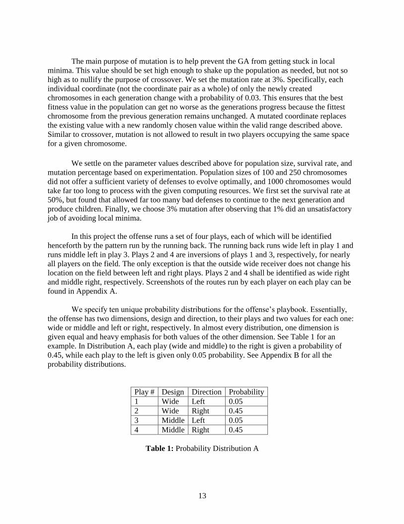
We specify ten unique probability distributions for the offense’s playbook. Essentially,
the offense has two dimensions, design and direction, to their plays and two values for each one:
wide or middle and left or right, respectively. In almost every distribution, one dimension is
given equal and heavy emphasis for both values of the other dimension. See Table 1 for an
example. In Distribution A, each play (wide and middle) to the right is given a probability of
0.45, while each play to the left is given only 0.05 probability. See Appendix B for all the
probability distributions.
Play # Design Direction Probability
1 Wide Left 0.05
2 Wide Right 0.45
3 Middle Left 0.05
4 Middle Right 0.45
Table 1: Probability Distribution A

14
4 Experiments
4.1 Player Attributes
Each player has a set of attributes that are assigned by their position. See Table 2. The
color of each position is used for easy identification. The zone radius indicates the
aggressiveness of a player to block defenders, in the case of an offensive player, or to pursue the
offense, in the case of a defensive player. The purpose of this parameter is described in greater
detail in the Implementation section above. It should be obvious that the defense is severely
handicapped. The fastest defensive players, safeties, are only half as fast as the quickest
offensive players, the running back and wide receivers. In fact, a safety has a speed of only 50,
while the slowest offensive player, an offensive lineman, has a speed of 40. Furthermore, a
defensive lineman has a zone radius of only 3, while his offensive counterpart has a zone radius
of 5. This means an offensive lineman reacts more quickly to blocking a defensive lineman than
the latter reacts to pursuing the offense. Also, since the mass of every player is set to 40 (not
shown in table), faster players can more easily push slower players out of place.
Originally, defensive players were set to have equivalent attribute values as their
offensive counterparts. After running some preliminary experiments, it became evident that the
defense performed far too well to be at all realistic. It was forcing the offense to lose several
yards on every play, and it would manage such performances after relatively few generations. It
was a challenge to set the player attributes to allow the offense to gain positive yards on average
while still allowing the defense to learn and defend effectively. The current values achieve a
reasonable balance, but even better settings may exist.
Table 2: Player attributes by position.
Position # Players Color Zone Radius Speed
OFFENSE
Running Back 1 Red N/A 100
Fullback 1 Yellow 6 90
Quarterback 1 Yellow 3 75
Wide Receiver 2 Yellow 8 100
Tight End 1 Yellow 5 50
Offensive Lineman 5 Yellow 5 40
DEFENSE
Defensive Lineman 4 Magenta 3 15
Linebacker 3 Cyan 6 30
Cornerback 2 Green 6 50
Safety 2 White 10 50
Total 22

15
4.2 Experimental Results
Based on our computational resources, we were able to run 50 generations for each of ten
probability distributions on the offense’s four plays. Ideally, we would have run multiple
iterations of 50 generations and averaged the results. This would reduce the variability in using a
non-guaranteed approach, namely a genetic algorithm, to find an optimal solution. Instead, we
report the results after 22 generations and 50 generations. We hope to find that the best
performing defense for a given probability distribution is the defense that was tuned on that
distribution.
We begin by discussing the results after 22 generations. Defense A is the best performing
defense, allowing 1.49 yards, on Distribution A, which places 90% emphasis on stopping plays
run right. Defense B was tuned on the opposite distribution, Distribution B, which puts 90%
emphasis on plays run left. Defense B allows 1.42 yards on Distribution B. The number of yards
allowed by each defense on its own distribution is approximately equal. Since we are minimizing
the sum of yards gained on each play, we expect Defenses A and B to allow a similar number of
yards on their respective distributions.
In contrast, we expect Defense A to do far worse on Distribution B than Defense B
performs on Distribution A. Defense A puts 0.45 weight on stopping the play wide right while
Defense B puts 0.45 weight on the wide left play. The difference is there is one wide receiver
blocking wide right and two wide receivers blocking wide left. Ignoring for a moment that we
are trying to minimize a weighted sum, a defense should allow fewer yards wide right than wide
left because it faces fewer blockers on the right side. Essentially, Defense A should perform
better wide right than Defense B performs wide left. This matches the data in Table 5, which
shows Defense A allowing -2.92 yards wide right, whereas Defense B allows -1.89 yards wide
left. By the same token, Defense A puts only 0.05 weight on the wide left play, and Defense B
puts 0.05 weight on the wide right play. Since the yardage allowed wide left contributes a very
small portion to the fitness of Defense A, it is likely to defend the left side with few players. This
means that the two wide receivers on the left side will likely push the sparse defenders back
several yards before the running back gets tackled. Similarly, the right side will contain few
defenders in Defense B, but there is only one wide receiver available for blocking. It is unlikely
that he will be as successful blocking the defenders as are two wide receivers. So we expect
Defense A to perform worse wide left than Defense B performs wide right, which is also
supported by the data in Table 5. Overall, the results of Defense A are more polarized, while
Defense B is more moderate. Consequently, Defense A should perform significantly worse than
Defense B on the opposite distribution. This result is supported by Table 3 and Table 4, which
show that Defense A allows 10.50 yards on Distribution B, while Defense B allows 5.99 yards
on Distribution A.

16
Defense Weighted Yardage
Allowed on Distribution A
A 1.48848
G 2.33069
E 2.47587
C 2.60386
J 2.70752
D 2.85566
H 2.90167
I 3.06664
F 4.91881
B 5.98732
Table 3: Defensive performances on Distribution A.
Defense Weighted Yardage
Allowed on Distribution B
B 1.41995
J 2.59902
H 2.89304
I 2.97561
F 3.52599
E 4.3197
G 4.72444
D 5.63078
C 6.40475
A 10.4955
Table 4: Defensive performances on Distribution B.
Plays Distribution A
Defense A Unweighted
Yardage Allowed Distribution B
Defense B Unweighted
Yardage Allowed
Wide Left 0.05 14.6195 0.45 -1.88529
Wide Right 0.45 -2.92489 0.05 4.49331
Middle Left 0.05 8.62318 0.45 3.58335
Middle Right 0.45 3.65011 0.05 8.62318
Table 5: Raw results of Defenses A and B.
Defense C is the second best performing defense on Distribution C, allowing just 0.72
yards. Only Defense H is better, allowing 0.57 yards. This result is not entirely alarming because
Distributions C and H are similar. While Distribution C puts 90% emphasis on plays run wide
and the remainder on plays run middle, Distribution H places 75% of the probability on wide
plays and 25% on middle plays. Defense D yields 2.86 yards, the fewest of any defense on

17
Distribution D. Note that Defense C allows a much smaller number of yards on its distribution
than does Defense D on its distribution. This indicates that it is more difficult for the defense to
tackle the running back when he runs up the middle as opposed to running wide. One reason for
this difference is that the routes of the blockers are much shorter when running up the middle,
allowing them to better adjust to blocking the defense. Conversely, on wide plays and in the case
of Defense C in particular, defenders can find a spot where they avoid being blocked (because
the blockers have not yet finished their routes), and still be in position to tackle the running back
as he approaches.
A counterintuitive reason why wide plays are easier to defend is due to the dominating
abilities of the offense. It is also attributable to the simple blocking scheme. A common scenario
on wide plays is the wide receiver aggressively blocks a defender. At the same time, he is
approached by another defender from the back side. Recall that an offensive player blocks the
closest defender in his zone radius. While battling the two defenders, the wide receiver may
become slightly more distanced from the original defender and, therefore, turn his attention to
blocking the backside defender. Since the wide receiver is among the fastest players on the field,
he will overpower any single defender. Unknowingly, the wide receiver may block the defender
into the running back, causing a yardage loss. This scenario is virtually impossible for plays run
up the middle because the running back gets to the line of scrimmage a fraction of a second
behind his lead blockers. There simply is insufficient time for the defense to sneak behind the
blockers and force themselves to be pushed into the running back. In summary, the potential of
the defense to limit yards is more restricted on middle plays than wide plays. This explains why
Defense C allows two fewer yards than Defense D on their respective distributions.
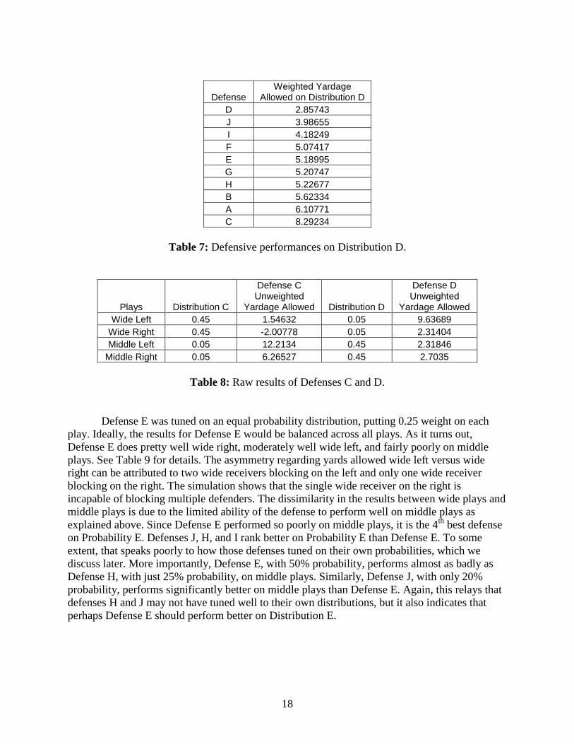
On Distribution D, Defense C gives up 8.29 yards, while Defense D allows 5.63 yards on
Distribution C. This is a greater discrepancy than we expected. Defense C’s results are mostly
unsurprising. It does very well wide right (-2.01 yards), moderately well wide left (1.55 yards),
and poorly middle left and right (12.21 yards and 6.27 yards respectively). On the other hand,
Defense D does about as well as can be expected on middle plays, allowing 2.32 yards middle
left and 2.70 yards middle right. It also performs poorly wide left as expected, giving up 9.64
yards. The surprise is that Defense D does pretty well wide right, allowing only 2.31 yards,
which is just as well as it did middle left. This unanticipated performance explains why Defense
D performs much better on Distribution C than vice versa.
Defense Weighted Yardage
Allowed on Distribution C
H 0.567941
C 0.716274
J 1.31999
E 1.60562
B 1.78393
G 1.84766
I 1.85976
F 3.37063
D 5.62901
A 5.87624
Table 6: Defensive performances on Distribution C.
18
Defense Weighted Yardage
Allowed on Distribution D
D 2.85743
J 3.98655
I 4.18249
F 5.07417
E 5.18995
G 5.20747
H 5.22677
B 5.62334
A 6.10771
C 8.29234
Table 7: Defensive performances on Distribution D.
Plays Distribution C
Defense C Unweighted
Yardage Allowed Distribution D
Defense D Unweighted
Yardage Allowed
Wide Left 0.45 1.54632 0.05 9.63689
Wide Right 0.45 -2.00778 0.05 2.31404
Middle Left 0.05 12.2134 0.45 2.31846
Middle Right 0.05 6.26527 0.45 2.7035
Table 8: Raw results of Defenses C and D.
Defense E was tuned on an equal probability distribution, putting 0.25 weight on each
play. Ideally, the results for Defense E would be balanced across all plays. As it turns out,
Defense E does pretty well wide right, moderately well wide left, and fairly poorly on middle
plays. See Table 9 for details. The asymmetry regarding yards allowed wide left versus wide
right can be attributed to two wide receivers blocking on the left and only one wide receiver
blocking on the right. The simulation shows that the single wide receiver on the right is
incapable of blocking multiple defenders. The dissimilarity in the results between wide plays and
middle plays is due to the limited ability of the defense to perform well on middle plays as
explained above. Since Defense E performed so poorly on middle plays, it is the 4th
best defense
on Probability E. Defenses J, H, and I rank better on Probability E than Defense E. To some
extent, that speaks poorly to how those defenses tuned on their own probabilities, which we
discuss later. More importantly, Defense E, with 50% probability, performs almost as badly as
Defense H, with just 25% probability, on middle plays. Similarly, Defense J, with only 20%
probability, performs significantly better on middle plays than Defense E. Again, this relays that
defenses H and J may not have tuned well to their own distributions, but it also indicates that
perhaps Defense E should perform better on Distribution E.

19
Defense Weighted Yardage
Allowed on Distribution E
J 2.65327
H 2.89736
I 3.02113
E 3.39779
G 3.52757
B 3.70364
F 4.2224
D 4.24322
C 4.5043
A 5.99198
Table 9: Defensive performances on Distribution E.
Plays Distribution E
Defense E Unweighted
Yardage Allowed
Wide Left 0.25 2.8351
Wide Right 0.25 -0.51994
Middle Left 0.25 6.26527
Middle Right 0.25 5.01072
Table 10: Raw results of Defense E.
Defense F is the 5th
best performing defense on Distribution F, obviously tuning poorly to
its distribution. Defense F allows 3.79 yards, more than 1.5 yards than the best performing
defense, Defense B. Looking at the play breakdown, it is clear why Defense F scores so poorly.
Defense F should allow the fewest yards wide left and middle left. Instead, it allows the fewest
yards wide left and wide right, and even those yardage allowances are not very good. Defense F
simply does not capitalize on the distribution’s strongest weights. It allows 4.31 yards middle
left, where Distribution F puts 0.375 weight. It is difficult to explain why the performance of
Defense F does not meet expectations.
Defense G yields 2.78 yards and ranks second best, just behind Defense J, on Distribution
G. Like Defense F, Defense G performs best on wide plays despite the distribution placing the
heaviest weights on plays to the right. The reason Defense G performs better than Defense F on
their respective distributions is that Defense G performs really well on one of the strong weights,
namely wide left, allowing negative yardage (-0.92).
Distribution F is similar to Distribution B and Distribution G is similar to Distribution A.
Consequently, we would expect the comparative results of Defenses F and G to be similar to
those of Defenses A and B. Specifically, we would expect Defenses F and G to perform equally
well on their own distributions, but Defense G should perform far worse on Distribution F than
vice versa for the same reasons as explained above for Defenses A and B. As it turns out, since
Defense F did not perform particularly well on any play, its overall results (3.79 yards) on

20
Distribution F are considerably worse than those of Defense G on Distribution G (2.78 yards). In
addition, Defense G actually performs better (4.28 yards) on Distribution F than Defense F does
on Distribution G (4.66 yards).
Defense Weighted Yardage
Allowed on Distribution F
B 2.27633
J 2.61936
H 2.89466
I 2.99268
F 3.78714
E 3.97398
G 4.27561
D 5.11045
C 5.69209
A 8.80666
Table 11: Defensive performances on Distribution F.
Defense Weighted Yardage
Allowed on Distribution G
J 2.68717
G 2.77952
E 2.82159
H 2.90005
I 3.04957
A 3.17729
C 3.31652
D 3.37599
F 4.65766
B 5.13094
Table 12: Defensive performances on Distribution G.
Plays Distribution F
Defense F Unweighted
Yardage Allowed Distribution G
Defense G Unweighted
Yardage Allowed
Wide Left 0.375 2.39481 0.125 3.78205
Wide Right 0.125 3.92056 0.375 -0.92668
Middle Left 0.375 4.30895 0.125 6.26527
Middle Right 0.125 6.26527 0.375 4.98963
Table 13: Raw results of Defenses F and G.
Defense H allows 1.44 yards and is the best defense for Distribution H, which places 0.75
weight on wide plays and 0.25 weight on middle plays. Defense I ranks third best on Distribution

21
I, giving up 3.75 yards. Since Distributions H and I are similar to Distributions C and D, we
expect parallel results. That is, Defense I should not do as well as Defense H on their respective
distributions because the capacity of the defense on middle plays is well restricted. By the same
token, we expect Defense H to perform worse on Distribution I than Defense I does on
Distribution H. Both of these are indeed true. Defense H yields 4.35 yards on Distribution I, and
Defense I gives up 2.30 yards on Distribution H. The only surprising element is that Defense I
performs better on Distribution H than Distribution I. This clearly indicates that Defense I did
not tune well to its distribution. However, unlike Defense F which also did not tune well,
Defense I ranks fairly well on its own distribution. Therefore, it must be difficult to score well on
Distribution I. This conclusion is reinforced by the fact that the best defense, Defense D, allows
3.38 yards on Distribution I, the most allowed by the best defense for any distribution. Since the
defense is minimizing a sum, Defense I must have found that while it could not further reduce
the yardage allowed on middle plays, it could decrease the yardage gain on wide plays. This
justifies how Defense I manages to score fairly well on Distribution I, but ultimately does better
on Distribution H.
Defense Weighted Yardage
Allowed on Distribution H
H 1.44147
J 1.81997
C 2.13679
E 2.27768
I 2.29527
G 2.47763
B 2.50382
F 3.69004
D 5.10934
A 5.91964
Table 14: Defensive performances on Distribution H.
Defense Weighted Yardage
Allowed on Distribution I
D 3.3771
J 3.48657
I 3.74698
H 4.35324
E 4.51789
G 4.57751
F 4.75475
B 4.90345
A 6.06431
C 6.87182
Table 15: Defensive performances on Distribution I.
22
Plays Distribution H
Defense H Unweighted
Yardage Allowed Distribution I
Defense I Unweighted
Yardage Allowed
Wide Left 0.375 -0.48135 0.125 2.68631
Wide Right 0.375 0.452526 0.125 0.452526
Middle Left 0.125 6.26527 0.375 3.24216
Middle Right 0.125 5.35298 0.375 5.7035
Table 16: Raw results of Defenses H and I.
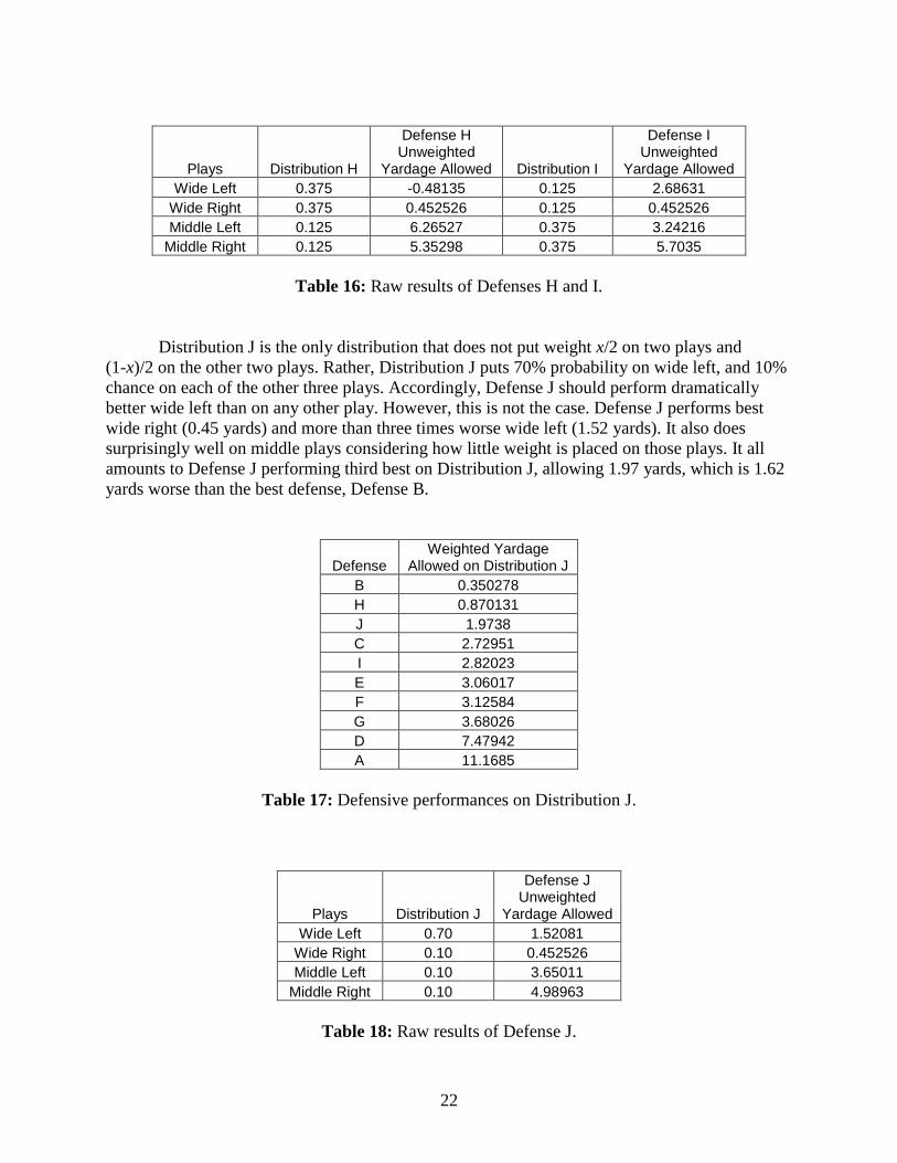
Distribution J is the only distribution that does not put weight x/2 on two plays and
(1-x)/2 on the other two plays. Rather, Distribution J puts 70% probability on wide left, and 10%
chance on each of the other three plays. Accordingly, Defense J should perform dramatically
better wide left than on any other play. However, this is not the case. Defense J performs best
wide right (0.45 yards) and more than three times worse wide left (1.52 yards). It also does
surprisingly well on middle plays considering how little weight is placed on those plays. It all
amounts to Defense J performing third best on Distribution J, allowing 1.97 yards, which is 1.62
yards worse than the best defense, Defense B.
Defense Weighted Yardage
Allowed on Distribution J
B 0.350278
H 0.870131
J 1.9738
C 2.72951
I 2.82023
E 3.06017
F 3.12584
G 3.68026
D 7.47942
A 11.1685
Table 17: Defensive performances on Distribution J.
Plays Distribution J
Defense J Unweighted
Yardage Allowed
Wide Left 0.70 1.52081
Wide Right 0.10 0.452526
Middle Left 0.10 3.65011
Middle Right 0.10 4.98963
Table 18: Raw results of Defense J.
23
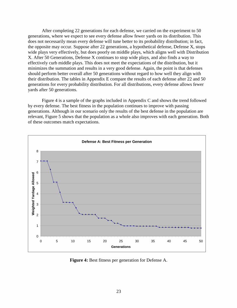
After completing 22 generations for each defense, we carried on the experiment to 50
generations, where we expect to see every defense allow fewer yards on its distribution. This
does not necessarily mean every defense will tune better to its probability distribution; in fact,
the opposite may occur. Suppose after 22 generations, a hypothetical defense, Defense X, stops
wide plays very effectively, but does poorly on middle plays, which aligns well with Distribution
X. After 50 Generations, Defense X continues to stop wide plays, and also finds a way to
effectively curb middle plays. This does not meet the expectations of the distribution, but it
minimizes the summation and results in a very good defense. Again, the point is that defenses
should perform better overall after 50 generations without regard to how well they align with
their distribution. The tables in Appendix E compare the results of each defense after 22 and 50
generations for every probability distribution. For all distributions, every defense allows fewer
yards after 50 generations.
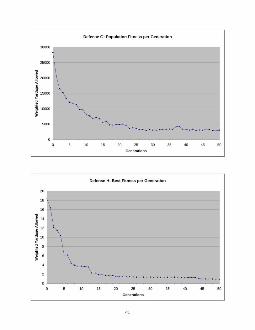
Figure 4 is a sample of the graphs included in Appendix C and shows the trend followed
by every defense. The best fitness in the population continues to improve with passing
generations. Although in our scenario only the results of the best defense in the population are
relevant, Figure 5 shows that the population as a whole also improves with each generation. Both
of these outcomes match expectations.
Defense A: Best Fitness per Generation
0
1
2
3
4
5
6
7
8
0 5 10 15 20 25 30 35 40 45 50
Generations
Weig
hte
d Y
ard
ag
e A
llo
wed
Figure 4: Best fitness per generation for Defense A.

24
Defense A: Population Fitness per Generation
0
5000
10000
15000
20000
25000
30000
0 5 10 15 20 25 30 35 40 45 50
Generations
Weig
hte
d Y
ard
ag
e A
llo
wed
Figure 5: Population fitness per generation for Defense A.
After completing 50 generations, we unexpectedly found that either Defense B or I
performs the best for every probability distribution. More specifically, Defense B ranks the best
for 7 of the 10 distributions, while Defense I is the best for the remaining three. A closer look
reveals that Defense B could potentially be declared the best overall defense. In addition to
owning 7 of 10 distributions, Defense B ranks second on the remaining three. On the other hand,
Defense I ranks from second down to seventh on the distributions where Defense B ranks first.
Furthermore, out of seven distributions, Defense B allows negative yardage on three of them.
See Appendix D for tables.
The key to Defense B’s dominance is a tremendous improvement where the distribution
weight is smallest. After 22 generations, Defense B allowed 4.49 yards and 8.62 yards on wide
right and middle right, respectively. After 50 generations, the yardage allowed is reduced to
-2.27 yards and 2.71 yards, respectively. Since Defense B performed well after 22 generations
where the distribution put the heaviest weight, there was not a great deal of room for
improvement on those plays. In fact, Defense B performs slightly worse on wide left after 50
generations (-1.78 yards) than it did after 22 generations (-1.89 yards). In exchange for this
minor decline, Defense B makes great strides on the remaining three plays. Another point to
notice is that Defense B does better wide right than wide left, despite Distribution B placing
more weight wide left. The simulator shows that Defense B exploits both the play design and the
blocking strategy. Not only is the single wide receiver on the right unable to push out the
multiple defenders, but he focuses on blocking the defender behind him and forces the defender
into the running back.

25
The story is quite different for Defense I. Recall that Defense I performed poorly after 22
generations where Distribution I placed the heaviest weights. After 50 generations, Defense I
finally figured out how to take advantage of the distribution’s weights and performs remarkably
well on middle plays (0.03 yards middle left and -0.30 yards middle right). In fact, it is the only
defense that causes a yardage loss on a middle play. This is surprising for two reasons: (1) As
has been stated previously, the defense is more handicapped on middle plays than wide plays by
virtue of the offensive blocking scheme and the lack of aggressiveness built in to the defensive
attacking strategy, and (2) Distribution D puts a heavier weight on middle plays than Distribution
I, but Defense D performs significantly worse on those plays than Defense I after 50 generations.
The reason Defense I is able to achieve negative yardage on a middle play is that it places a
defender next to the line of scrimmage where he does not get blocked because another defender
attracts the attention of the blockers. Like Defense B, Defense I does worse wide left after 50
generations (2.05 yards) than it did after 22 generations (-0.48 yards). However, this does not
greatly affect Defense I because Distribution I puts only 0.125 weight on the wide left play; the
improvement on the middle plays significantly outweighs the decline wide left.
Plays Distribution B
Defense B Unweighted
Yardage Allowed Distribution I
Defense I Unweighted
Yardage Allowed
Wide Left 0.45 -1.78831 0.125 2.0459
Wide Right 0.05 -2.27164 0.125 0.452526
Middle Left 0.45 2.61474 0.375 0.0267963
Middle Right 0.05 2.71133 0.375 -0.295881
Table 19: Raw results of Defenses B and I.
It is a challenge to explain why Defenses B and I do the best across all distributions after
50 generations. We expected that after 50 generations, every defense would perform the best for
the distribution on which it was tuned. Obviously, that did not turn out to be the case. Rather, it
seems that Defenses B and I found a way to break out of local minima better than all other
defenses. The genetic algorithm used in this experiment employs a great deal of randomness. If
we had the opportunity to run the entire experiment multiple times, we could average the results
and determine whether it was a fluke that Defenses B and I did so well or whether their
distributions truly foster dominant defenses.
5 Summary and Future Work
In this work, we make two contributions: (1) a graphical simulator to optimize defenses for
the game of American football, and (2) optimized defenses for a variety of game situations. The
simulator can be configured with relative ease to include more waypoints in the route design,
different colors for the environment and players, different camera angles, and a number of other
parameters. Moreover, the simulator is completely independent of the learning algorithm. We

26
use a genetic algorithm to optimize defenses, but any other optimization method could be
substituted.
The experimental results showed that defenses tuned on a distribution with a 90-10
balance of weights (Defenses A-D) rank the best for their distribution after 22 generations. The
results are less consistent for defenses tuned on 75-25 weights (Defenses F-H). After 50
generations, we find that either Defense B or I does the best for every probability distribution.
Perhaps the first step in continuing work on this domain would be to run the experiment
multiple times and average the results to form firmer conclusions. It may help to run each
defense for more than 50 generations. In addition, the simulator could be extended to allow
richer football scenarios (i.e. pass plays) and more realistic player behavior, such as improved
blocking and a more intelligent defensive attack strategy. Furthermore, the GA could search over
not only player locations, but also over player instructions, such as zone versus man defense.
Finally, we are curious how a different optimization strategy, such as simulated annealing, would
compare to the results achieved by a genetic algorithm.

27
References
[1] AGEIA. http://www.ageia.com.
[2] OpenGL – The Industry’s Foundation for High Performance Graphics.
http://www.opengl.org/about/overview.
[3] OpenGL Utility Toolkit – Wikipedia, the free encyclopedia.
http://en.wikipedia.org/wiki/GLUT.
[4] The Football Dictionary. http://library.thinkquest.org/12590/dictionary.htm.
[5] DiscoverHover :: Curriculum Guides :: Glossary of Terms.
http://www.discoverhover.org/infoinstructors/vocab.htm.
[6] Euler Integration – Wikipedia, the free encyclopedia.
http://en.wikipedia.org/wiki/Euler_integration.
[7] Mitchell, Melanie. An Introduction to Genetic Algorithms. Prentice-Hall of India Private
Limited. October 2002.

28
Appendix A: Player Routes
Provided are screenshots of the routes for each offensive player on each play. Fewer than
five waypoints can be seen for some players because their waypoints are repeated, effectively
shortening their route. The defense has been excluded from these screenshots for clarity.
Key
RB Running Back
FB Fullback
QB Quarterback
C Center
LG Left Guard
LT Left Tackle
RG Right Guard
RT Right Tackle
TE Tight End
IWR Inside Wide Receiver
OWR Outside Wide Receiver

29
Play 1: Wide Left
RT RG
C
RB
LG LT
TE OWR
FB IWR QB

30
Play 2: Wide Right
OWR RB FB
RT RG C LG LT
TE
IWR QB

31
Play 3: Middle Left
RT
RG C
LG LT
TE
OWR
RB FB IWR QB

32
Play 4: Middle Right
RT RG C LG LT
TE OWR
RB FB
IWR
QB

33
Appendix B: Probability Distributions
The ten probability distributions are provided here for quick reference. They are also
included in Tables 5, 8, 10, 13, 16, and 18.
Play Distribution A Distribution B Distribution C Distribution D Distribution E
Wide Left 0.05 0.45 0.45 0.05 0.25
Wide Right 0.45 0.05 0.45 0.05 0.25
Middle Left 0.05 0.45 0.05 0.45 0.25
Middle Right 0.45 0.05 0.05 0.45 0.25
Play Distribution F Distribution G Distribution H Distribution I Distribution J
Wide Left 0.375 0.125 0.375 0.125 0.70
Wide Right 0.125 0.375 0.375 0.125 0.10
Middle Left 0.375 0.125 0.125 0.375 0.10
Middle Right 0.125 0.375 0.125 0.375 0.10

34
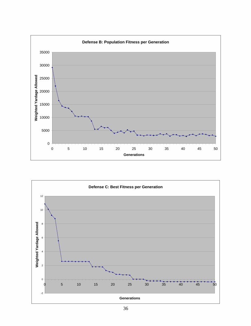
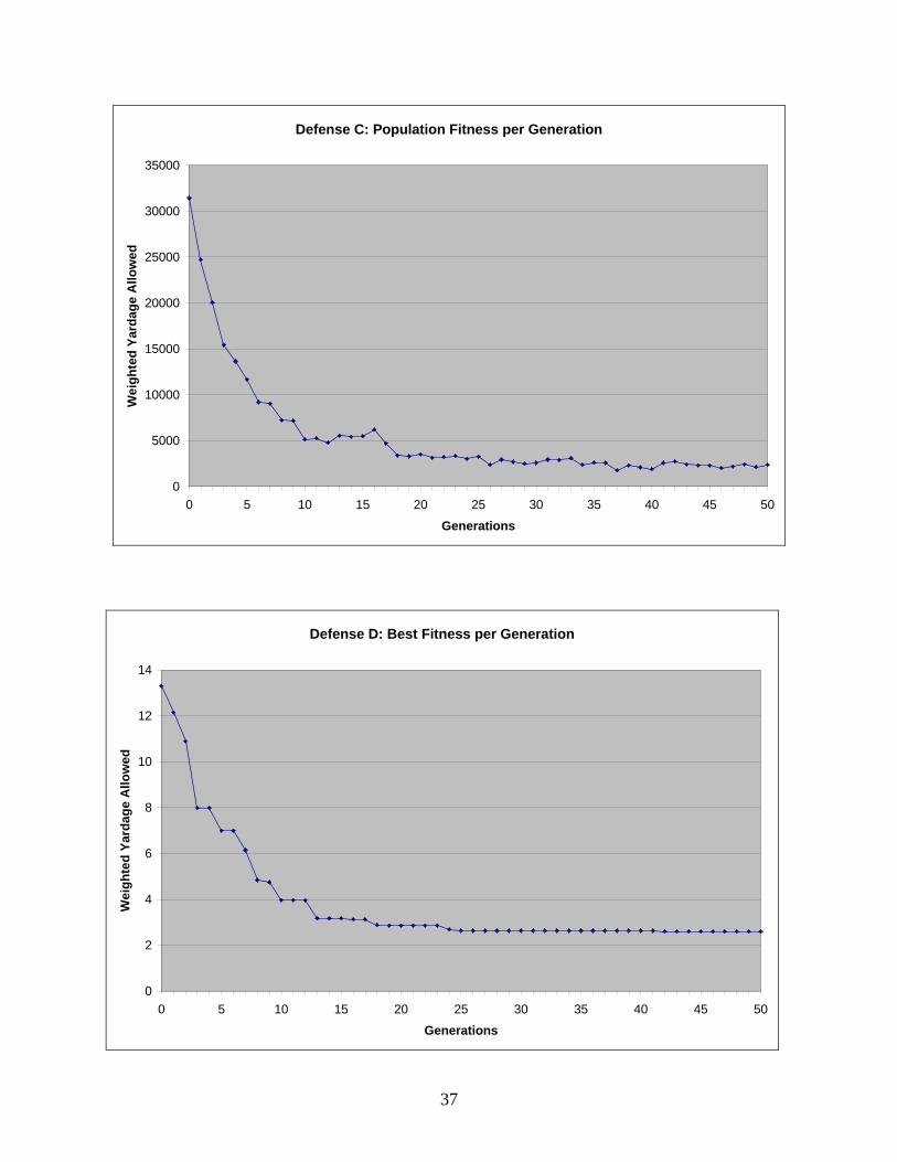
Appendix C: Fitness Graphs
Included here are graphs of Best Fitness per Generation and Population Fitness per
Generation for each defense on its own distribution.
Defense A: Best Fitness per Generation
0
1
2
3
4
5
6
7
8
0 5 10 15 20 25 30 35 40 45 50
Generations
We
igh
ted
Yard
ag
e A
llo
we
d

35
Defense A: Population Fitness per Generation
0
5000
10000
15000
20000
25000
30000
0 5 10 15 20 25 30 35 40 45 50
Generations
We
igh
ted
Yard
ag
e A
llo
we
d
Defense B: Best Fitness per Generation
0
2
4
6
8
10
12
14
16
0 5 10 15 20 25 30 35 40 45 50
Generations
Weig
hte
d Y
ard
ag
e A
llo
wed
36
Defense B: Population Fitness per Generation
0
5000
10000
15000
20000
25000
30000
35000
0 5 10 15 20 25 30 35 40 45 50
Generations
We
igh
ted
Yard
ag
e A
llo
we
d
Defense C: Best Fitness per Generation
-2
0
2
4
6
8
10
12
0 5 10 15 20 25 30 35 40 45 50
Generations
We
igh
ted
Yard
ag
e A
llo
we
d
37
Defense C: Population Fitness per Generation
0
5000
10000
15000
20000
25000
30000
35000
0 5 10 15 20 25 30 35 40 45 50
Generations
Weig
hte
d Y
ard
ag
e A
llo
wed
Defense D: Best Fitness per Generation
0
2
4
6
8
10
12
14
0 5 10 15 20 25 30 35 40 45 50
Generations
Weig
hte
d Y
ard
ag
e A
llo
wed

38
Defense D: Population Fitness per Generation
0
5000
10000
15000
20000
25000
30000
0 5 10 15 20 25 30 35 40 45 50
Generations
Weig
hte
d Y
ard
ag
e A
llo
wed
Defense E: Best Fitness per Generation
0
2
4
6
8
10
12
14
0 5 10 15 20 25 30 35 40 45 50
Generations
We
igh
ted
Yard
ag
e A
llo
we
d

39
Defense E: Population Fitness per Generation
0
5000
10000
15000
20000
25000
30000
35000
0 5 10 15 20 25 30 35 40 45 50
Generations
We
igh
ted
Yard
ag
e A
llo
we
d
Defense F: Best Fitness per Generation
0
5
10
15
20
25
0 5 10 15 20 25 30 35 40 45 50
Generations
We
igh
ted
Yard
ag
e A
llo
we
d

40
Defense F: Population Fitness per Generation
0
5000
10000
15000
20000
25000
30000
35000
0 5 10 15 20 25 30 35 40 45 50
Generations
Weig
hte
d Y
ard
ag
e A
llo
wed
Defense G: Best Fitness per Generation
0
2
4
6
8
10
12
14
16
18
0 5 10 15 20 25 30 35 40 45 50
Generations
We
igh
ted
Yard
ag
e A
llo
we
d
41
Defense G: Population Fitness per Generation
0
5000
10000
15000
20000
25000
30000
0 5 10 15 20 25 30 35 40 45 50
Generations
We
igh
ted
Yard
ag
e A
llo
we
d
Defense H: Best Fitness per Generation
0
2
4
6
8
10
12
14
16
18
20
0 5 10 15 20 25 30 35 40 45 50
Generations
Weig
hte
d Y
ard
ag
e A
llo
wed

42
Defense H: Population Fitness per Generation
0
5000
10000
15000
20000
25000
30000
35000
0 5 10 15 20 25 30 35 40 45 50
Generations
We
igh
ted
Yard
ag
e A
llo
we
d
Defense I: Best Fitness per Generation
0
1
2
3
4
5
6
7
8
9
0 5 10 15 20 25 30 35 40 45 50
Generations
Weig
hte
d Y
ard
ag
e A
llo
wed

43
Defense I: Population Fitness per Generation
0
5000
10000
15000
20000
25000
30000
0 5 10 15 20 25 30 35 40 45 50
Generations
We
igh
ted
Yard
ag
e A
llo
we
d
Defense J: Best Fitness per Generation
0
2
4
6
8
10
12
14
16
18
20
0 5 10 15 20 25 30 35 40 45 50
Generations
Weig
hte
d Y
ard
ag
e A
llo
wed

44
Defense J: Population Fitness per Generation
0
5000
10000
15000
20000
25000
30000
35000
0 5 10 15 20 25 30 35 40 45 50
Generations
We
igh
ted
Yard
ag
e A
llo
we
d

45
Appendix D: Defensive Performances After 50 Generations
The tables provided here show the performance of each defense for a given probability
distribution after 50 generations.
Defense Weighted Yardage
Allowed on Distribution A
I 0.174125
B 0.239184
A 0.774904
E 1.00507
G 1.15986
C 1.3042
J 1.34502
H 2.43017
D 2.60011
F 3.17017
Defense Weighted Yardage
Allowed on Distribution B
B 0.393877
I 0.940544
H 1.25415
F 1.93694
J 2.44723
E 2.56418
C 3.21126
D 3.52659
A 4.07327
G 4.20109
Defense Weighted Yardage
Allowed on Distribution C
B -1.56067
C -0.358676
J 0.200841
H 0.353766
G 0.560995
E 0.56348
I 1.11084
A 1.80924
F 2.04227
D 3.52482

46
Defense Weighted Yardage
Allowed on Distribution D
I 0.00383291
B 2.19373
D 2.60188
E 3.00578
A 3.03893
F 3.06483
H 3.33056
J 3.59141
G 4.79996
C 4.87414
Defense Weighted Yardage
Allowed on Distribution E
B 0.316531
I 0.557334
E 1.78463
H 1.84216
J 1.89612
C 2.25773
A 2.42409
F 2.55355
G 2.68048
D 3.06335
Defense Weighted Yardage
Allowed on Distribution F
B 0.364872
I 0.79684
H 1.47466
F 2.16817
J 2.24056
E 2.27185
C 2.85369
D 3.35288
A 3.45483
G 3.63086

47
Defense Weighted Yardage
Allowed on Distribution G
B 0.268189
I 0.317828
E 1.29741
A 1.39335
J 1.55168
C 1.66177
G 1.73009
H 2.20967
D 2.77382
F 2.93893
Defense Weighted Yardage
Allowed on Distribution H
B -0.856722
C 0.622477
J 0.836572
I 0.903273
H 0.911914
E 1.02141
G 1.3558
A 2.03981
F 2.234
D 3.35177
Defense Weighted Yardage
Allowed on Distribution I
I 0.211396
B 1.48978
E 2.54785
H 2.77241
D 2.77493
A 2.80837
F 2.8731
J 2.95567
C 3.89299
G 4.00515
48
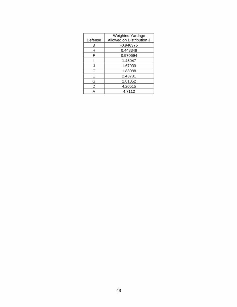
Defense Weighted Yardage
Allowed on Distribution J
B -0.946375
H 0.443349
F 0.970694
I 1.45047
J 1.67039
C 1.83088
E 2.43731
G 2.81052
D 4.20515
A 4.7112

49
Appendix E: Comparison of Distribution Rankings In the Experimental Results section, we provide tables for how each defense performs on
a given distribution. Here we provide a different perspective. The tables included here show how
a given defense performs on each probability distribution. The results are in ascending order of
yardage allowed.
22 Generations 50 Generations
Distribution Weighted Yardage
Allowed by Defense A
Distribution Weighted Yardage
Allowed by Defense A
A 1.48848 A 0.774904
G 3.17729 G 1.39335
C 5.87624 C 1.80924
H 5.91964 H 2.03981
E 5.99198 E 2.42409
I 6.06431 I 2.80837
D 6.10771 D 3.03893
F 8.80666 F 3.45483
B 10.4955 B 4.07327
J 11.1685 J 4.7112
22 Generations 50 Generations
Distribution Weighted Yardage
Allowed by Defense B
Distribution Weighted Yardage
Allowed by Defense B
J 0.350278 C -1.56067
B 1.41995 J -0.946375
C 1.78393 H -0.856722
F 2.27633 A 0.239184
H 2.50382 G 0.268189
E 3.70364 E 0.316531
I 4.90345 F 0.364872
G 5.13094 B 0.393877
D 5.62334 I 1.48978
A 5.98732 D 2.19373
22 Generations 50 Generations
Distribution Weighted Yardage
Allowed by Defense C
Distribution Weighted Yardage
Allowed by Defense C
C 0.716274 C -0.358676
H 2.13679 H 0.622477
A 2.60386 A 1.3042
J 2.72951 G 1.66177
G 3.31652 J 1.83088
E 4.5043 E 2.25773
F 5.69209 F 2.85369
B 6.40475 B 3.21126
I 6.87182 I 3.89299
D 8.29234 D 4.87414

50
22 Generations 50 Generations
Distribution Weighted Yardage
Allowed by Defense D
Distribution Weighted Yardage
Allowed by Defense D
A 2.85566 A 2.60011
D 2.85743 D 2.60188
G 3.37599 G 2.77382
I 3.3771 I 2.77493
E 4.24322 E 3.06335
H 5.10934 H 3.35177
F 5.11045 F 3.35288
C 5.62901 C 3.52482
B 5.63078 B 3.52659
J 7.47942 J 4.20515
22 Generations 50 Generations
Distribution Weighted Yardage
Allowed by Defense E
Distribution Weighted Yardage
Allowed by Defense E
C 1.60562 C 0.56348
H 2.27768 A 1.00507
A 2.47587 H 1.02141
G 2.82159 G 1.29741
J 3.06017 E 1.78463
E 3.39779 F 2.27185
F 3.97398 J 2.43731
B 4.3197 I 2.54785
I 4.51789 B 2.56418
D 5.18995 D 3.00578
22 Generations 50 Generations
Distribution Weighted Yardage
Allowed by Defense F
Distribution Weighted Yardage
Allowed by Defense F
J 3.12584 J 0.970694
C 3.37063 B 1.93694
B 3.52599 C 2.04227
H 3.69004 F 2.16817
F 3.78714 H 2.234
E 4.2224 E 2.55355
G 4.65766 I 2.8731
I 4.75475 G 2.93893
A 4.91881 D 3.06483
D 5.07417 A 3.17017

51
22 Generations 50 Generations
Distribution Weighted Yardage
Allowed by Defense G
Distribution Weighted Yardage
Allowed by Defense G
C 1.84766 C 0.560995
A 2.33069 A 1.15986
H 2.47763 H 1.3558
G 2.77952 G 1.73009
E 3.52757 E 2.68048
J 3.68026 J 2.81052
F 4.27561 F 3.63086
I 4.57751 I 4.00515
B 4.72444 B 4.20109
D 5.20747 D 4.79996
22 Generations 50 Generations
Distribution Weighted Yardage
Allowed by Defense H
Distribution Weighted Yardage
Allowed by Defense H
C 0.567941 C 0.353766
J 0.870131 J 0.443349
H 1.44147 H 0.911914
B 2.89304 B 1.25415
F 2.89466 F 1.47466
E 2.89736 E 1.84216
G 2.90005 G 2.20967
A 2.90167 A 2.43017
I 4.35324 I 2.77241
D 5.22677 D 3.33056
22 Generations 50 Generations
Distribution Weighted Yardage
Allowed by Defense I
Distribution Weighted Yardage
Allowed by Defense I
C 1.85976 D 0.00383291
H 2.29527 A 0.174125
J 2.82023 I 0.211396
B 2.97561 G 0.317828
F 2.99268 E 0.557334
E 3.02113 F 0.79684
G 3.04957 H 0.903273
A 3.06664 B 0.940544
I 3.74698 C 1.11084
D 4.18249 J 1.45047

52
22 Generations 50 Generations
Distribution Weighted Yardage
Allowed by Defense J
Distribution Weighted Yardage
Allowed by Defense J
C 1.31999 C 0.200841
H 1.81997 H 0.836572
J 1.9738 A 1.34502
B 2.59902 G 1.55168
F 2.61936 J 1.67039
E 2.65327 E 1.89612
G 2.68717 F 2.24056
A 2.70752 B 2.44723
I 3.48657 I 2.95567
D 3.98655 D 3.59141

53
Appendix F: Simulator Instructions
There are three versions of the football simulator. While all of them are essentially the
same, they each have different inputs and outputs that focus it to a specific purpose. The main,
and most important, simulator is the one that employs a genetic algorithm and uses the results of
the simulation to evolve better defenses. We altered the main simulator to create a second
simulator, one that automatically evaluates all defenses on all probability distributions. The third
simulator is primarily intended for investigative purposes. We use this manual evaluation
simulator to gain better understanding of the interactions between offense and defense. For
example, this simulator was used to design offensive plays and determine how defenses were
causing yardage losses.
The main simulator expects one or two input files. The first and required argument
specifies a probability distribution. This file can have any name, but it must match the format
shown in Figure F1. Each line of the input must specify the play number, play design, play
direction, and the probability expressed as a decimal. The sum of the probabilities for the plays
must be 1. The amount of white space does not matter, but we use a single tab between words.
The number of plays in this file should match the number of plays specified as a global constant
in the code. The second input file is required to continue the genetic algorithm where it left off.
This is useful for gathering results after x number of executions and then continuing processing
for analysis at further generations, much like we reported results after 22 and 50 generations.
This file is generated as part of the output during processing and is described in more detail
below. The simulator continues processing from the generation, chromosome, and play where it
was interrupted. We do not recommend stopping the simulator between generations while
crossover and mutation are occurring, as these are not replicated on continuation.
Figure F1: Sample input file to main simulator. This file specifies a probability distribution.
The main simulator writes output to the console for easy visual inspection and also prints
to four text files. Every output file contains a header that provides details on a variety of GA
parameter settings, such as the population size, survival rate, and mutation rate. This header is
printed every time the GA starts processing, including manual continuations. As each generation
completes processing, the entire population of chromosomes is appended to
GA_all_placements.txt. This is useful in the event that we need to compare the performance of
multiple chromosomes within a given generation. GA_fitness.txt provides information on the
best fitness, population fitness, and processing time for each generation. This file is used to graph
trend information regarding the progress of the GA. GA_raw_data.txt contains the raw yardage
allowed on every play for every chromosome and generation. It also includes the best fitness,
population fitness, and execution time for each generation. In addition, it gives details on
1 wide left 0.70
2 wide right 0.10
3 middle left 0.10
4 middle right 0.10
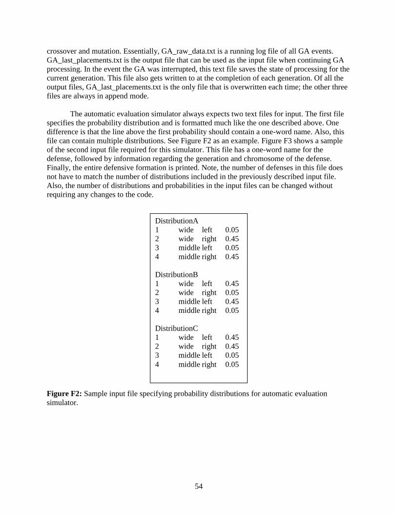
54
crossover and mutation. Essentially, GA_raw_data.txt is a running log file of all GA events.
GA_last_placements.txt is the output file that can be used as the input file when continuing GA
processing. In the event the GA was interrupted, this text file saves the state of processing for the
current generation. This file also gets written to at the completion of each generation. Of all the
output files, GA_last_placements.txt is the only file that is overwritten each time; the other three
files are always in append mode.
The automatic evaluation simulator always expects two text files for input. The first file
specifies the probability distribution and is formatted much like the one described above. One
difference is that the line above the first probability should contain a one-word name. Also, this
file can contain multiple distributions. See Figure F2 as an example. Figure F3 shows a sample
of the second input file required for this simulator. This file has a one-word name for the
defense, followed by information regarding the generation and chromosome of the defense.
Finally, the entire defensive formation is printed. Note, the number of defenses in this file does
not have to match the number of distributions included in the previously described input file.
Also, the number of distributions and probabilities in the input files can be changed without
requiring any changes to the code.
Figure F2: Sample input file specifying probability distributions for automatic evaluation
simulator.
DistributionA
1 wide left 0.05
2 wide right 0.45
3 middle left 0.05
4 middle right 0.45
DistributionB
1 wide left 0.45
2 wide right 0.05
3 middle left 0.45
4 middle right 0.05
DistributionC
1 wide left 0.45
2 wide right 0.45
3 middle left 0.05
4 middle right 0.05

55
Figure F3: Sample input file specifying defenses for the automatic evaluation simulator.
The automatic evaluation simulator writes two text output files. The first line of
rawEvaluations.txt defines how the raw yardage is computed. The rest of the file includes the
raw yardage allowed by each defense on each play. Figure F4 shows a sample output file based
on the input given in Figure F3. The second file, summaryEvaluations.txt, contains the fitness
values of all defenses sorted in ascending order for each probability distribution. This file also
has the fitness of each defense sorted in ascending order on all distributions. Given the input files
in Figures F3 and F4, Figure F5 shows the sample output file.
Figure F4: Sample output file (rawEvaluations.txt) containing raw yardage data.
DefenseA
Gen# 50 Chrom# 0
18 24 21 24 24 27 27 15 27 21 24
24 6 27 24 -9 -27 6 24 -24 -6 -24
0.774904 0 0 0 0 0 0 0 0 0 0
DefenseB
Gen# 50 Chrom# 0
24 27 27 24 27 27 27 24 24 21 27
6 -3 -24 -6 -6 6 24 30 -21 24 -27
0.393877 0 0 0 0 0 0 0 0 0 0
Raw yardage definition: Running Back yards gained relative to line of scrimmage
Defense_v3.8a
Gen# 50 Chrom# 0
Play: 1 RawYardage: 6.23594
Play: 2 RawYardage: -2.92489
Play: 3 RawYardage: 2.73519
Play: 4 RawYardage: 3.65011
Defense_v3.8b
Gen# 50 Chrom# 0
Play: 1 RawYardage: -1.78831
Play: 2 RawYardage: -2.27164
Play: 3 RawYardage: 2.61474
Play: 4 RawYardage: 2.71133
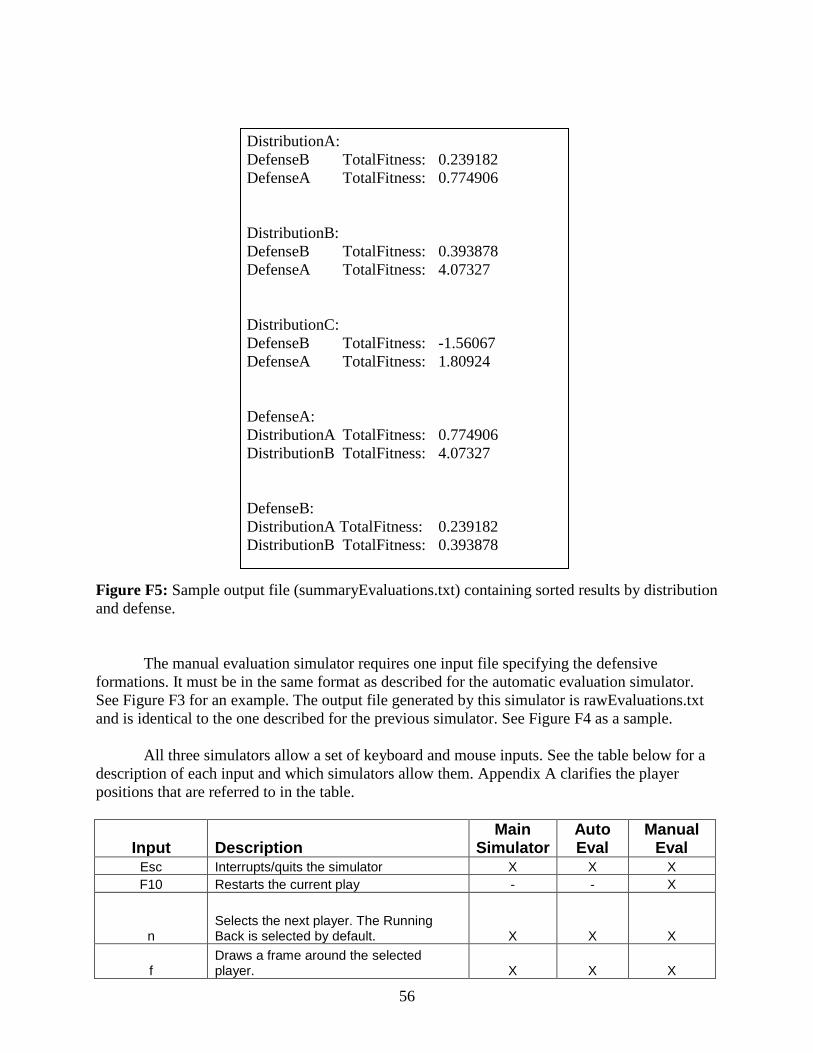
56
Figure F5: Sample output file (summaryEvaluations.txt) containing sorted results by distribution
and defense.
The manual evaluation simulator requires one input file specifying the defensive
formations. It must be in the same format as described for the automatic evaluation simulator.
See Figure F3 for an example. The output file generated by this simulator is rawEvaluations.txt
and is identical to the one described for the previous simulator. See Figure F4 as a sample.
All three simulators allow a set of keyboard and mouse inputs. See the table below for a
description of each input and which simulators allow them. Appendix A clarifies the player
positions that are referred to in the table.
Input Description Main
Simulator Auto Eval
Manual Eval
Esc Interrupts/quits the simulator X X X
F10 Restarts the current play - - X
n Selects the next player. The Running Back is selected by default. X X X
f Draws a frame around the selected player. X X X
DistributionA:
DefenseB TotalFitness: 0.239182
DefenseA TotalFitness: 0.774906
DistributionB:
DefenseB TotalFitness: 0.393878
DefenseA TotalFitness: 4.07327
DistributionC:
DefenseB TotalFitness: -1.56067
DefenseA TotalFitness: 1.80924
DefenseA:
DistributionA TotalFitness: 0.774906
DistributionB TotalFitness: 4.07327
DefenseB:
DistributionA TotalFitness: 0.239182
DistributionB TotalFitness: 0.393878

57
c Prints the environment coordinates of the player to the console. X X X
t Prints the player type or position to the console. X X x
p Pauses play execution. - - X
i Advances to the next defense. - - X
> Advances to the next play. Wraps around from last play to first play. - - X
< Returns to the previous play. Wraps around from first play to last play. - - X
0 Toggles drawing the route of the Running Back. X X X
1 Toggles drawing the route of the Center. X X X
2 Toggles drawing the route of the Left Guard. X X X
3 Toggles drawing the route of the Left Tackle. X X X
4 Toggles drawing the route of the Right Guard. X X X
5 Toggles drawing the route of the Right Tackle. X X X
6 Toggles drawing the route of the Tight End. X X X
7 Toggles drawing the route of the outside Wide Receiver. X X X
8 Toggles drawing the route of the inside Wide Receiver. X X X
9 Toggles drawing the route of the Quarterback. X X X
- (dash)
Toggles drawing the route of the Fullback. X X X
= Toggles drawing of all routes. X X X
~ Clears drawing of all routes. X X X
w Zooms in camera. X X X
s Zooms out camera. X X X
q Moves camera up (from initial perspective). X X X
z Moves camera down (from initial perspective). X X X
a Moves camera left. X X X
d Moves camera right. X X X
Mouse Left-Click & Drag Rotates camera. X X X