simulation-based uncertainty quantification of human ... · simulation-based uncertainty...
TRANSCRIPT

INTERNATIONAL JOURNAL FOR NUMERICAL METHODS IN BIOMEDICAL ENGINEERINGInt. J. Numer. Meth. Biomed. Engng. 2013; 00:1–24Published online in Wiley InterScience (www.interscience.wiley.com). DOI: 10.1002/cnm
Simulation-based uncertainty quantification of human arterialnetwork hemodynamics
Peng Chen1,∗, Alfio Quarteroni1,2, Gianluigi Rozza3
1Modelling and Scientific Computing, CMCS, Mathematics Institute of Computational Science and Engineering,MATHICSE, Ecole Polytechnique Federale de Lausanne, EPFL, Station 8, CH-1015 Lausanne, Switzerland.
2 Modellistica e Calcolo Scientifico, MOX, Dipartimento di Matematica F. Brioschi, Politecnico di Milano, P.zaLeonardo da Vinci 32, I-20133, Milano, Italy.
3 SISSA MathLab, International School for Advanced Studies, via Bonomea 265, 34136 Trieste, Italy.
SUMMARY
This work aims at identifying and quantifying uncertainties from various sources in human cardiovascularsystem based on stochastic simulation of a one dimensional arterial network. A general analysis ofdifferent uncertainties and probability characterization with log-normal distribution of these uncertaintiesis introduced. Deriving from a deterministic one dimensional fluid structure interaction model, we establishthe stochastic model as a coupled hyperbolic system incorporated with parametric uncertainties to describethe blood flow and pressure wave propagation in the arterial network. By applying a stochastic collocationmethod with sparse grid technique, we study systemically the statistics and sensitivity of the solution withrespect to many different uncertainties in a relatively complete arterial network with potential physiologicaland pathological implications for the first time. Copyright c© 2013 John Wiley & Sons, Ltd.
Received . . .
KEY WORDS: uncertainty quantification, sensitivity analysis, stochastic collocation method, cardiovas-cular modelling, human arterial network, wave propagation, hemodynamics
1. INTRODUCTION
Mathematical modelling and numerical simulation of human cardiovascular system have undergonea vast development over the last few decades thanks to better understanding of the morphologyand functionality of cardiovascular system, the availability of abundant clinical data as wellas fast growing of computational resources [38, 23]. Specifically, various deterministic modelstargeted for the full human arterial tree, or specific sites (e.g. the carotid bifurcation, the aorticarch etc.), have been established [23, 2]. For instance, Navier-Stokes equations and elastic orviscoelastic equations are coupled together to characterize the fluid structure interaction propertybetween the blood flow and the arterial wall in three dimensional configurations [23]; the onedimensional hyperbolic system simplified from the full three dimensional equations together withappropriate coupling conditions at the vascular junctions are widely used to describe the bloodflow and pressure wave propagation phenomena in the arterial tree; geometrical multiscale modelscoupling the macrosvascular network (large arterials), mesovascular network (medium or smallarterials) as well as microvascular network (arterioles or capillaries) are investigated for the
∗Correspondence to: Modelling and Scientific Computing, CMCS, Mathematics Institute of Computational Scienceand Engineering, MATHICSE, Ecole Polytechnique Federale de Lausanne, EPFL, Station 8, CH-1015 Lausanne,Switzerland. Email: [email protected]
Copyright c© 2013 John Wiley & Sons, Ltd.Prepared using cnmauth.cls [Version: 2010/03/27 v2.00]

2 P. CHEN, A. QUARTERONI, G. ROZZA
hope to simulate systemically the physiological blood flow in the entire human vascular network[30, 24, 28]. Moreover, models for tissue perfusion [18], mass transfer [50], bypass design [40],electromechanical activity of the heart [14] and so on have also been developed with specificobjectives. Meanwhile, various efficient computational techniques [20, 35, 9, 8, 23, 17, 27] havealso enhanced greatly for the cardiovascular modelling and simulation.
However, there are always discrepancies between measurements and the deterministic simulationresults, since many uncertainties exist in cardiovascular system due to its complexity, diversity andvariability [23]. For instance, the evolution of cerebral aneurysm can be influenced evidently byrandom external pressure or inflows [43]; the development of carotid atherosclerosis might be highlyrelated to the inhomogeneous randomly distributed components of blood as well as the patternof blood flow, whose geometry may be uncertain in a large degree due to the accumulation offatty material [38]. Some of the uncertainties, namely epistemic uncertainties, can be reduced bymore precise measurement or more advanced noise filtering techniques, while the other of them,namely aleatory uncertainties, are very difficult if not impossible to be accurately captured due to theinhomogeneous and multiscale properties of the cardiovascular system that undergoes an instantlyand intrinsically variation owing to, for instance, the surrounding tissue pressure or external workforce [23]. To identify and quantify these uncertainties, even if partially, and incorporate them intothe well developed deterministic models will benefit not only for more accurate modelling andsimulation of the cardiovascular system, but also for better understanding of the cardiovasculardiseases. Therefore, development and analysis of efficient computational methods for uncertaintyquantification becomes very important for mathematical modelling and numerical simulation ofcardiovascular system.
In the modelling of the complex cardiovascular system, uncertainties are inevitably encounteredfrom various sources and may play an important role in computational simulation. When it comes tomathematical modelling, these uncertainties may be classified in general in the following categories:
1. Computational geometries: Blood flow in the vascular system and the heart depends on thegeometry of the blood lumen and blood vessel, which could be uncertain in a large extent,e.g., for what concerns, branch separation or bifurcation, high deflection bends, arterial wallthickness, lumen narrowed down by atherosclerosis or balloon-like bulge in the wall due toaneurysms. In fact, geometrical noise typically comes from the reconstruction of the geometryof the blood vessel with data from medical image devices, such as CT or MRI [38].
2. Mathematical models: There have been many mathematical models built in differentgeometrical scales and for different physical properties. Depending on the computationalgeometry, we may have multiscale models accounting for the detailed or simplified fluidvelocity field and pressure with rigid or compliant walls. Based on the physical properties,we can characterize blood flow with Newtonian or non-Newtonian rheology, with or withoutviscoelastic or inertial properties, etc. [23]. Uncertainties thus arise from adoption of differentmathematical models.
3. Physical parameters: When the mathematical model is established, the coefficients orphysical parameters in the mathematical model is exposed to various uncertainties due tocrude or unavailable measurements. The outcome of the blood flow simulation is undoubtedlydetermined at a certain extent by these physical parameters accounting for material propertiesof fluid and structure, such as the permeability, elasticity, compliance or Young’s modulus ofthe arterial wall, the diffusivity of substance dissolved in the inhomogeneous blood solventand so on [50].
4. Boundary conditions: Even for the same mathematical model and the same physicalparameters, the confidence in the output of the computational simulation also depends on theuncertainties of boundary conditions prescribed on the boundary of the computational domain,including the inlet velocities or flow flux, outlet resistance or lumped parameter models, theinteraction on the interface between the lumen and the arterial wall, etc [43].
5. External sources or forces: The transport of the main substance is carried by the blood,which also contains some other substances that make the chemical reaction between thesedifferent and contacting substances possible, resulting in increase or decrease of the substance
Copyright c© 2013 John Wiley & Sons, Ltd. Int. J. Numer. Meth. Biomed. Engng. (2013)Prepared using cnmauth.cls DOI: 10.1002/cnm

SIMULATION-BASED UNCERTAINTY QUANTIFICATION OF HUMAN ARTERIAL NETWORK 3
of interest. Meanwhile, the flow rate of the blood is influenced by the surrounding tissue oruncertain distribution of external work force, which may also lead to the variation of the bloodflow [23].
In order to have more precise characterization and interpretation of the cardiovascular systemby mathematical modelling and numerical simulation, these uncertainties must be taken intoaccount with different emphasis depending on the purpose. How to identify and propagate theinfluential uncertainties in the mathematical modelling on different levels is still at the beginningof investigation [43, 2, 49]. In fact, there is no mature techniques to characterize and representthese heterogeneous uncertainties arising from different sources, let alone systematic analysis of theinfluence of them to the cardiovascular system. Preliminary work has been carried out for parametricuncertainty quantification in a local region or part of the vascular network with only one or two typesof parameters [43, 49]. The authors in [43] proposed an adaptive stochastic collocation frameworkfor uncertainty quantification and propagation in cardiovascular simulations. They studied the radiusof the abdominal aortic aneurysm, the radius and inflow velocity of the carotid artery bifurcationas well as flow split of the LPA/RPA as random variables following either Gaussian or uniformdistribution to account for the uncertainty impact on blood flow modelled by three dimensionalNavier-Stokes equations with rigid arterial wall in a small region. A main part of the vascularnetwork with 37 arterial segments with independent and uniformly distributed parameters for eachsegment was described by a one dimensional stochastic model by the authors in [49]. In particular,they considered the sensitivity of pressure with respect to the uncertainty of material parameter(e.g. Young modulus) in different segments and apply generalized polynomial chaos combined withstochastic collocation method to compute the solution.
In this work, we concentrate on and highlight the following three aspects for uncertaintyquantification in the human arterial tree: 1, we first investigate several parametric uncertaintiesindependently for time dependent sensitivity and stochastic convergence analysis; 2, and then westudy systemically many different sources of parametric uncertainties (around 10) listed aboveat the same time and examine their distinct importance to cardiovascular simulation via globalsensitivity analysis; 3, we also consider parameter dependent boundary conditions (resistance) ineach distal boundary site and geometrical parameter (cross-section area) in each arterial segmentobeying independent and identical probability distribution to unveil the most important region wherethe uncertainty is located for the quantity of interest. For this set of preliminary and explanatoryanalyses, we build a one dimensional stochastic fluid structure interaction model for the systemicarterial tree based on a one dimensional deterministic model validated by clinical measurements[39]. Although it couldn’t be applied to study the local flow fields as in three dimensional modellingwith detailed geometry, e.g. secondary flow, wall shear stress, vorticity of the velocity field, we aresatisfied with this simplified one dimensional model for the fact that it is intrinsically a coupledhyperbolic system suitable to describe the blood flow and pressure wave propagation in the globalvascular network. Moreover, we consider the vascular network with great completeness of thesystemic circulation, incorporating the detailed description of the cerebral and coronary arteries,wall viscoelastic properties, wall friction and convection acceleration effect as well as realistic distalboundary conditions at the terminal sites characterized by three element windkessel model [39, 29].These advantages enable us in a large extent to carry out more realistic uncertainty quantification inthe global vascular network with many parameters.
In section 2 we summarize the deterministic fluid structure interaction model of the humanarterial tree with brief description of the coupling condition and the lumped parameter model for theterminal boundary as well as the basic numerical approximation scheme. Based on the deterministicmodel we formulate the stochastic model in the probability framework and introduce the stochasticcollocation method to solve the stochastic system. Criteria for statistical and sensitivity analysisare defined according to the representation of stochastic collocation solution. In section 3, westudy the statistics and sensitivity of the solution with respect to different uncertainties in threeaspects: 1, stochastic regularity and nonlinearity of the solution as well as the convergence analysisof the collocation method in the case of one dimensional parametric uncertainty; 2, systemic timeaveraged and time dependent sensitivity analysis of all the uncertainties over one heart beat in the
Copyright c© 2013 John Wiley & Sons, Ltd. Int. J. Numer. Meth. Biomed. Engng. (2013)Prepared using cnmauth.cls DOI: 10.1002/cnm
4 P. CHEN, A. QUARTERONI, G. ROZZA
case of moderate (10) dimensional parametric uncertainty; 3, quantification of the dependence ofuncertainty location with independent random variables to account for uncertainty of resistance ateach distal boundary and reference area in each arterial segment in the case of high (47 and 103)dimensional parametric uncertainty.
2. MATHEMATICAL MODELLING OF THE HUMAN ARTERIAL TREE
2.1. Deterministic modelling: one dimensional fluid structure interaction
We introduce the simplified one dimensional deterministic fluid structure interaction modelto describe the blood flow in arteries and its interaction with the blood vessel displacementfollowing [22, 36]. In the absence of bifurcation, each segment of the arteries can be consideredas a cylindrical compliant and impermeable tube with cross section S(t, x), being t ∈ (0, T ] thetime and x ∈ [0, L] the axial coordinate. The radius r of the tube and the pressure P of theblood flow are assumed to be functions of only t and x. We also assume that the velocity u ofthe blood flow is dominated in the axial coordinate and depends on t, x and r with the profiles(r, θ) = θ−1(θ + 2)(1− rθ), where we have θ = 2 for parabolic Poiseuille profile, θ = 9 for morephysiological Womersley profile and θ →∞ for a simple flat profile [23]. The state variables forthe study of wave propagation phenomena, namely the cross-sectional area A, the volumetric flowrate Q and the average pressure P , are defined by
A(t, x) =
∫S(t,x)
dS, Q(t, x) =
∫S(t,x)
uxdS, P (t, x) =1
A
∫S(t,x)
PdS. (1)
By integrating the three dimensional Navier-Stokes equations on a generic section S and replacingthe velocity and pressure by the state variables defined in (1) (see [36, 23, 29] for details), we obtainthe following simplified one dimensional equations governed by mass and momentum conservationlaw
∂A
∂t+∂Q
∂x= 0 in (0, T ]× [0, L],
∂Q
∂t+
∂
∂x
(αQ2
A
)+A
ρ
∂P
∂x+ kr
Q
A= 0 in (0, T ]× [0, L],
(2)
where the second term and the fourth term of the momentum equation account for the convectiveacceleration effect and the wall friction effect, respectively. α and kr are the Coriolis coefficient andfriction coefficient defined as
α =1
A
∫S(t,x)
s2dS, kr = −2πµ
ρ
ds
dr
∣∣∣r=1
, (3)
being µ the kinematic viscosity, ρ the blood density and r = 1 on the arterial wall.In order to close the fluid system (2) consisting of two equations and three variables A,Q and P ,
we need to provide an additional relation between the pressure and the wall deformation and thusthe cross section area according to certain constitutive law of the arterial wall, for instance [36]
P − Pext = ψ(A) + ψ(A) := β
(√A
A0− 1
)+ γ
(1
A√A
∂A
∂t
), (4)
which incorporates not only the elastic effect in the first term but also the viscoelastic effect in thesecond term. The coefficients β and γ entail the physical parameters for the material property of thearterial wall in the following formula
β =
√π
A0
hE
1− ν2, γ =
T tanφ
4√π
hE
1− ν2, (5)
Copyright c© 2013 John Wiley & Sons, Ltd. Int. J. Numer. Meth. Biomed. Engng. (2013)Prepared using cnmauth.cls DOI: 10.1002/cnm

SIMULATION-BASED UNCERTAINTY QUANTIFICATION OF HUMAN ARTERIAL NETWORK 5
where h,E, ν,A0 are the wall thickness, Young modulus, Poisson coefficient and referencesectional area under only external pressure Pext; the viscoelastic parameters T and φ are the wavecharacteristic time and angle determining the viscoelasticity effect. More complex wall models canalso be employed by taking into account inertia, longitudinal elasticity, etc. [22]. Initial conditionsfor system (2) can be chosen in the reference state, being A = A0, Q = 0 and P = Pext or any otherstate with data extracted from either numerical simulations or clinical measurements [23].
For numerical approximation of system (2), we apply operator splitting techniques, decomposingthe volumetric flow rate into two parts Q = Q+ Q that account for the elastic effect and theviscoelastic effect respectively, and rewrite (2) for the elastic component in the conservationform [29]
∂U
∂t+∂F (U)
∂x+ S(U) = 0 in (0, T ]× [0, L], (6)
where U = [A,Q]T and U = [A, Q]T are the total and conservative variables, F = [Q,F2]T are thecorresponding fluxes with
F2 =
∫ A
A0
A
ρ
∂ψ
∂AdA+ α
Q2
A, (7)
and S = [0, S2]T consists of the friction and the non-uniformity of the geometry and the materialwith
S2 = krQ
A+A
ρ
(∂ψ
∂A0
∂A0
∂x+∂ψ
∂β
∂β
∂x
)− ∂
∂A0
∫ A
A0
A
ρ
∂ψ
∂AdA
∂A0
∂x− ∂
∂β
∫ A
A0
A
ρ
∂ψ
∂AdA
∂β
∂x. (8)
As for the viscoelastic part, we obtain from system (2)
1
A
∂Q
∂t− ∂
∂x
(γ
ρA3/2
∂Q
∂x
)= 0 in (0, T ]× [0, L]. (9)
There have been several numerical discretization schemes applied to approximate (6) and (9),e.g. second order Taylor-Galerkin [22], discontinuous Galerkin [44], spectral/hp element [49]. Wechoose the second order Taylor-Galerkin finite element approximation for simplicity, which is moreconvenient to deal with the operator splitting techniques [29]. It can be shown [36] that (6) is afirst order non-linear hyperbolic system so that some compatibility condition is needed to enablethe computation of state variables at the first and last nodes. Moreover, the system (6) and (9) areclosed by imposing valid boundary conditions, such as physiological flow rate, terminal absorbingconditions or lumped parameter models, for instance, the three element windkessels consisting oftwo resistors and one capacitor described by the ordinary differential equation
P − Pv + CR2dP
dt= (R1 +R2)Q+ CR1R2
dQ
dtin (0, T ], (10)
where Pv is the prescribed venous pressure, C is the capacitance and R1, R2 are the resistances withthe common relation R1 = 4R/5, R2 = R/5 where R = R1 +R2 is the total resistance [39].
The one dimensional fluid structure interaction model (2) and (4) together with proper initial andboundary conditions is among the most popular way to describe the blood flow and its interactionwith the arterial wall in each arterial segment locally [39]. In order to construct all the segmentsstructurally and functionally to form the human arterial tree, suitable coupling conditions are neededat the bifurcations. It is demonstrated in [22] that a domain decomposition approach by keeping themass conservation and total pressure continuity are satisfactory for characterizing blood velocityand pressure wave propagation without evident dissipation of energy in the arterial branching. Moreexplicitly, supposing there are Np proximal segments and Nd distal segments at a certain joint, weimpose the following equations for the proximal and distal state variables (Qp, P p) and (Qd, P d)
Np∑n=1
Qpn =
Nd∑m=1
Qdm, and P pn = P dm, ∀n = 1, . . . , Np,m = 1, . . . , Nd. (11)
Copyright c© 2013 John Wiley & Sons, Ltd. Int. J. Numer. Meth. Biomed. Engng. (2013)Prepared using cnmauth.cls DOI: 10.1002/cnm
6 P. CHEN, A. QUARTERONI, G. ROZZA
This approach can be realized numerically by nonlinear Richardson strategy, using Newton orinexact Newton method combined with Broyden algorithm for updating Jacobian matrix, see [29]for details.
2.2. Stochastic modelling: quantifying uncertainties
As introduced in section 1, there are many different kinds of uncertainties arising from diversesources of the human arterial tree with distinct features. Among several possible approaches todescribe these uncertainties, e.g., evident theory, fuzzy set theory, probability theory, the latter onesprovide a general framework to characterize various uncertainties more precisely in a quantitativeway [7, 5]. Roughly speaking, we employ the concept of random variable in probability theory torandomize a deterministic variable or parameter, e.g. the reference area A0(x) ∈ R, x ∈ [0, L], toa real-valued random variable depending also on some outcome ω of a set of probability eventsΩ, i.e. A0(x, ω) ∈ R, x ∈ [0, L], ω ∈ Ω. Once the deterministic variable is replaced by a randomvariable, the model consisting of (6), (9) and (10) becomes a stochastic model. In order to solvethe stochastic model, we first take a series of stochastic realization A0(x, ωn), n = 1, 2, . . . , Naccording to certain prescribed probability distribution, then solve a deterministic model for eachA0(x, ωn), n = 1, 2, . . . , N . For the sake of evaluating statistics of the stochastic solution, e.g.expectation or mean value where we need to compute an integral of the solution with respect to aprobability distribution, we use properly selected quadrature formulas based on a set of collocationpoints and weights, which is called stochastic collocation method [4]. When the number of randomvariables becomes large, for instance K random variables, we need NK collocation points forthe full tensor product stochastic collocation method, yielding NK deterministic models to solve,which is computationally prohibitive especially when the solution of a single deterministic model isexpensive. In this case, we employ sparse grid stochastic collocation method [32], i.e. select somerepresentative collocation points to form a sparse grid to alleviate considerably the computationaleffort. In general, this method features more accurate and efficient evaluation of the statistics ofstochastic solution. Let us introduce the procedure more rigorously.
Given a complete probability space (Ω,F ,P), which consists of the set of outcomes Ω, the σ-algebra of events F and a probability measure P : F → [0, 1], we can define a random variableY : Ω→ R such that for every Borel set B ⊂ R we have Y −1(B) = ω∈ Ω : Y (ω) ∈ B ∈ F .Provided that the random variable depends also on temporal or spatial coordinate, we have stochasticprocess or random fields [7]. The stochastic system of the one dimensional fluid structure interactionmodel corresponding to the deterministic system (6), (9) and (10) becomes: find the stochastic stateprocesses (A,Q,P ) : (0, T ]× [0, L]× Ω→ R3, such that P-almost surely the following equationshold with proper initial boundary conditions:
∂U
∂t(t, x, ω) +
∂F (U)
∂x(t, x, ω) + S(U)(t, x, ω) = 0 in (0, T ]× [0, L]× Ω,
1
A
∂Q
∂t(t, x, ω)− ∂
∂x
(γ
ρA3/2
∂Q
∂x
)(t, x, ω) = 0 in (0, T ]× [0, L]× Ω,
P (t, ω)− Pv + CR2dP
dt(t, ω) = (R1 +R2)Q(t, ω) + CR1R2
dQ
dt(t, ω) in (0, T ]× Ω.
(12)For each realization ω ∈ Ω, we assume that the stochastic system (12) shares the same mathematicalproperties as its deterministic counterpart, in particular, being still a hyperbolic system. Thestochasticity of the state variables is propagated from the random inputs accounting for theuncertainties of involved parameters in the system, including the geometrical parameters, physicalparameters as well as parameters arising from boundary conditions and external pressure. Theseparameters can be either represented by random variables or stochastic processes following certainprobability distributions. In order to calibrate the probability distributions from various datasources such as literatures, measurements or experts’ opinions, we may employ statistical inferencetechniques, for instance, linear and nonlinear regression, maximum likelihood estimation, maximumentropy, etc. [19, 46].
Copyright c© 2013 John Wiley & Sons, Ltd. Int. J. Numer. Meth. Biomed. Engng. (2013)Prepared using cnmauth.cls DOI: 10.1002/cnm
SIMULATION-BASED UNCERTAINTY QUANTIFICATION OF HUMAN ARTERIAL NETWORK 7
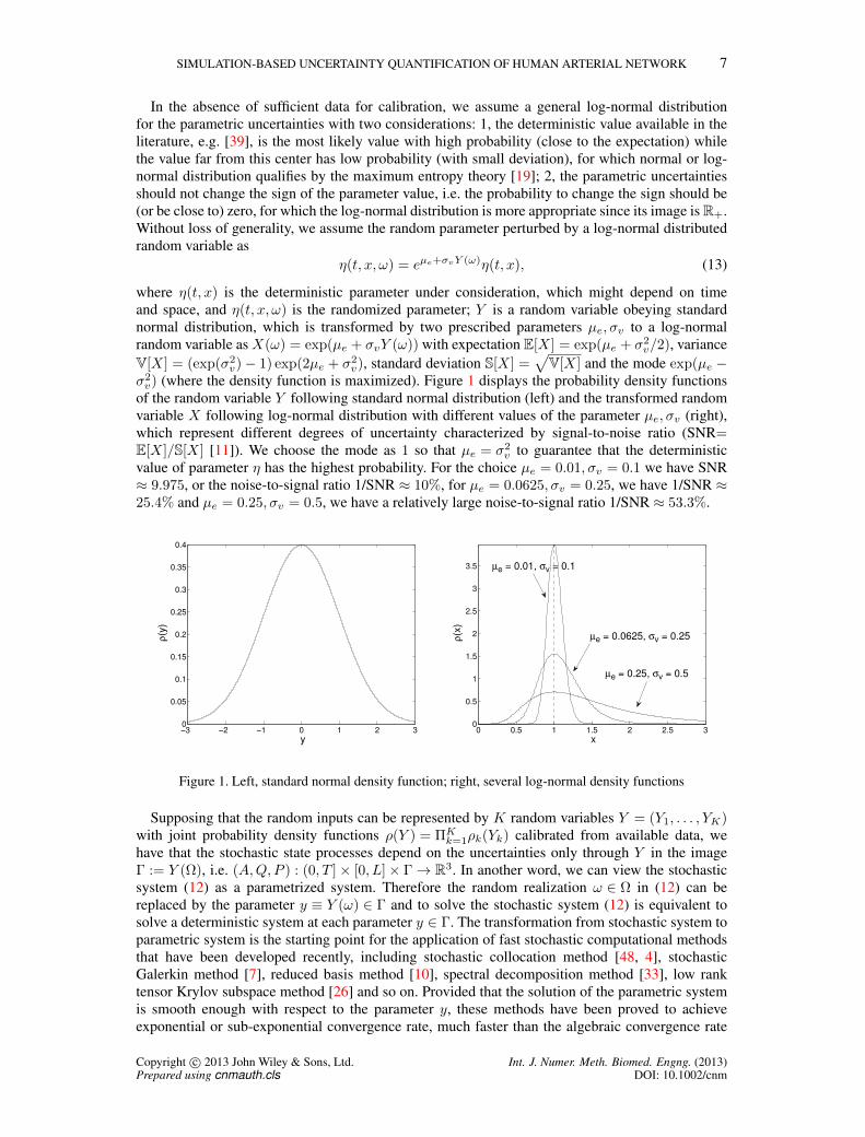
In the absence of sufficient data for calibration, we assume a general log-normal distributionfor the parametric uncertainties with two considerations: 1, the deterministic value available in theliterature, e.g. [39], is the most likely value with high probability (close to the expectation) whilethe value far from this center has low probability (with small deviation), for which normal or log-normal distribution qualifies by the maximum entropy theory [19]; 2, the parametric uncertaintiesshould not change the sign of the parameter value, i.e. the probability to change the sign should be(or be close to) zero, for which the log-normal distribution is more appropriate since its image is R+.Without loss of generality, we assume the random parameter perturbed by a log-normal distributedrandom variable as
η(t, x, ω) = eµe+σvY (ω)η(t, x), (13)
where η(t, x) is the deterministic parameter under consideration, which might depend on timeand space, and η(t, x, ω) is the randomized parameter; Y is a random variable obeying standardnormal distribution, which is transformed by two prescribed parameters µe, σv to a log-normalrandom variable as X(ω) = exp(µe + σvY (ω)) with expectation E[X] = exp(µe + σ2
v/2), varianceV[X] = (exp(σ2
v)− 1) exp(2µe + σ2v), standard deviation S[X] =
√V[X] and the mode exp(µe −
σ2v) (where the density function is maximized). Figure 1 displays the probability density functions
of the random variable Y following standard normal distribution (left) and the transformed randomvariable X following log-normal distribution with different values of the parameter µe, σv (right),which represent different degrees of uncertainty characterized by signal-to-noise ratio (SNR=E[X]/S[X] [11]). We choose the mode as 1 so that µe = σ2
v to guarantee that the deterministicvalue of parameter η has the highest probability. For the choice µe = 0.01, σv = 0.1 we have SNR≈ 9.975, or the noise-to-signal ratio 1/SNR ≈ 10%, for µe = 0.0625, σv = 0.25, we have 1/SNR ≈25.4% and µe = 0.25, σv = 0.5, we have a relatively large noise-to-signal ratio 1/SNR ≈ 53.3%.
−3 −2 −1 0 1 2 30
0.05
0.1
0.15
0.2
0.25
0.3
0.35
0.4
y
ρ(y
)
0 0.5 1 1.5 2 2.5 30
0.5
1
1.5
2
2.5
3
3.5
x
ρ(x
)
µe = 0.0625, σv = 0.25
µe = 0.25, σv = 0.5
µe = 0.01, σv = 0.1
Figure 1. Left, standard normal density function; right, several log-normal density functions
Supposing that the random inputs can be represented by K random variables Y = (Y1, . . . , YK)with joint probability density functions ρ(Y ) = ΠK
k=1ρk(Yk) calibrated from available data, wehave that the stochastic state processes depend on the uncertainties only through Y in the imageΓ := Y (Ω), i.e. (A,Q,P ) : (0, T ]× [0, L]× Γ→ R3. In another word, we can view the stochasticsystem (12) as a parametrized system. Therefore the random realization ω ∈ Ω in (12) can bereplaced by the parameter y ≡ Y (ω) ∈ Γ and to solve the stochastic system (12) is equivalent tosolve a deterministic system at each parameter y ∈ Γ. The transformation from stochastic system toparametric system is the starting point for the application of fast stochastic computational methodsthat have been developed recently, including stochastic collocation method [48, 4], stochasticGalerkin method [7], reduced basis method [10], spectral decomposition method [33], low ranktensor Krylov subspace method [26] and so on. Provided that the solution of the parametric systemis smooth enough with respect to the parameter y, these methods have been proved to achieveexponential or sub-exponential convergence rate, much faster than the algebraic convergence rate
Copyright c© 2013 John Wiley & Sons, Ltd. Int. J. Numer. Meth. Biomed. Engng. (2013)Prepared using cnmauth.cls DOI: 10.1002/cnm

8 P. CHEN, A. QUARTERONI, G. ROZZA
N−1/2 of Monte-Carlo method [21]. Moreover, stochastic collocation method, similar to Monte-Carlo method, turns out more applicable for nonlinear and complex system due to its non-intrusivefeature that enables us to use the deterministic solver directly and repeatedly without mathematicalreformulation [6, 15].
Given the collocation points in Γ ⊂ R, e.g.,−∞ < y0 < y1 < y2 < · · · < yN <∞ as well as thecorresponding functions f(yn), 0 ≤ n ≤ N (state variables (A,Q,P ) in our context), we define theunivariate N th order Lagrangian interpolation
UNf(y) =
N∑n=0
f(yn)ln(y), where ln(y) =∏m6=n
y − ym
yn − ym0 ≤ n ≤ N. (14)
Rewrite the univariate interpolation formula (14) with the index k for the kth dimension as
UNkf(yk) =
∑ynkk ∈Θk
f(ynk
k )lnk
k (yk), where Θk = ynk
k ∈ Γk, nk = 0, . . . , Nk for some Nk ≥ 1
(15)then the multivariate interpolation is given as the tensor product of the univariate interpolation
(UN1⊗ · · · ⊗ UNK
) f(y) =∑
yn11 ∈Θ1
· · ·∑
ynKK ∈ΘK
f(yn11 , . . . , ynK
K )(ln11 (y1)⊗ · · · ⊗ lnK
K (yK)). (16)
In order to alleviate the “curse of dimensionality” in the interpolation on the full tensor product gridfor high dimensional problems, we employ the Smolyak sparse grid interpolation that considerablyreduces the number of the total collocation nodes by removing most of the cross-dimensionalcollocation nodes in an optimizing way while keeping high order interpolation in each dimension[45]. It achieves fast convergence rate without much sacrifice of accuracy compared to the samelevel of the full tensor product interpolation, in particular for analytic problem, and is proven tobe one of the most efficient and widely used stochastic collocation methods [48, 32]. The generalSmolyak formula reads
Sqf(y) =∑
q−K+1≤|i|≤q
(−1)q−|i|(K − 1q − |i|
)(U i1 ⊗ · · · ⊗ U iK
)f(y), (17)
where |i| = i1 + · · ·+ iK with the multivariate index i = (i1, . . . , iK) defined via the two possiblesets
Xs(q,K) :=
i ∈ NK
+ ,∀ ik ≥ 1 :
K∑k=1
ik ≤ q
or Xp(q,K) :=
i ∈ NK
+ ,∀ ik ≥ 1 :
K∏k=1
ik ≤ q
(18)
and the set of collocation nodes of the sparse grid is thus collected as
H(q,K) =⋃
q−K+1≤|i|≤q
(Θi1 × · · · ×ΘiK
), (19)
where #Θik = 1 if ik = 1, and #Θik = 2ik−1 + 1 when ik > 1 in a nested structure. Note that wedenote U ik ≡ UNk
defined in (15) for Nk = 2ik−1. We define q −K as the level of interpolation.Figure 2 depicts the full tensor product grid, sparse grid with index setsXs(q,K) andXp(q,K) withcollocations nodes defined as Gauss-Hermite quadrature abscissas [13] for two independent randomvariables obeying standard normal distribution, from which we can observe a large reduction of thetotal number of collocation nodes, especially for the sparse grid with index set Xp(q,K). Moreadvanced techniques, such as anisotropic sparse grid [31], sparse grid constructed via hierarchicalsurplus [25] and reduced basis [15], have been developed by taking advantage of stochasticregularity and a posteriori error estimate for further reduction of the computational cost.
Copyright c© 2013 John Wiley & Sons, Ltd. Int. J. Numer. Meth. Biomed. Engng. (2013)Prepared using cnmauth.cls DOI: 10.1002/cnm

SIMULATION-BASED UNCERTAINTY QUANTIFICATION OF HUMAN ARTERIAL NETWORK 9
−4 −3 −2 −1 0 1 2 3 4−4
−3
−2
−1
0
1
2
3
4
−4 −3 −2 −1 0 1 2 3 4−4
−3
−2
−1
0
1
2
3
4
−4 −3 −2 −1 0 1 2 3 4−4
−3
−2
−1
0
1
2
3
4
Figure 2. Two dimensional (K = 2) full tensor product grid (left, 81 nodes) and sparse grid with index setXs(q,K) (middle, 49 nodes) and index set Xp(q,K) (right, 25 nodes), all the collocation nodes are chosen
as Gauss-Hermite quadrature abscissas with the level of interpolation q −K = 3
By repeatedly solving a deterministic system at each collocation node (19), we can constructan explicit formula for the stochastic state variables at any parameter y ∈ Γ via the sparse gridinterpolation (17). In practice, we are more interested in the evaluation of the statistics of the statevariables, such as expectation or variance, which can be computed straightforwardly as
E[f ] ≈ E[Sqf ] =
∫Γ
Sqf(y)ρ(y)dy =∑
q−K+1≤|i|≤q
(−1)q−|i|(K − 1q − |i|
)E[(U i1 ⊗ · · · ⊗ U iK
)f]
(20)where the tensor product expectation can be evaluated by the following quadrature formula
E[(UN1 ⊗ · · · ⊗ UNK) f ] =
∑yn11 ∈Θ1
· · ·∑
ynKK ∈ΘK
f(yn11 , . . . , ynK
K )(wn1
1 × · · · × wnK
K
), (21)
being (ynk
k , wnk
k ), 1 ≤ k ≤ K the quadrature abscissas and weights according to the joint probabilitydistribution function and UNk
≡ U ik , 1 ≤ k ≤ K. The evaluation of variance is computed by
V[f ] = E[(f − E[f ])2
]≈ E
[Sqf2
]−(E[Sqf ]
)2. (22)
In order to improve the accuracy of the numerical integral in (20) and the numerical interpolationin (17), it is favourable to select the collocation points as the quadrature abscissas. Availablequadrature rules include Clenshaw-Curtis quadrature (with Chebshev Gauss Lobatto nodes),Gaussian quadrature based on various orthogonal polynomials and so on [37, 32].
Another interest is to study the sensitivity of the state variables with respect to differentparameters, or in another word, how the solution depends on each parameter at some realizationy ∈ Γ, namely local or pointwise sensitivity analysis [41], as well as how much weight that theuncertainty arising from each parameter contributes to the total variation of the solution in the nameof global sensitivity analysis [42, 12]. In the uncertainty quantification of the human arterial tree, weare more interested in how different parameters affect the blood flow and pressure wave propagationsystemically, therefore, the global sensitivity analysis. Following [12], we define the variance basedglobal sensitivity index - main effect of the kth parameter as
Gk[f ] =V[E[f |yk]]
V[f ], k = 1, . . . ,K, (23)
where V[E[f |yk]] is the variance of the expectation of the variable f conditioned on the kthparameter yk, accounting for the contribution to the total variance of the solution by this parameter.More explicitly, it can be evaluated approximately via the sparse grid interpolation by
V[E[f |yk]] ≈∫
Γk
(∫Γ∗k
Sqf(y)ρ(y∗k)dy∗k
)2
ρ(yk)dyk −(∫
Γ
Sqf(y)ρ(y)dy
)2
, (24)
Copyright c© 2013 John Wiley & Sons, Ltd. Int. J. Numer. Meth. Biomed. Engng. (2013)Prepared using cnmauth.cls DOI: 10.1002/cnm

10 P. CHEN, A. QUARTERONI, G. ROZZA
where yk is the kth element of y in one dimensional parameter space Γk and y∗k is the adjointcounterpart or all the other elements of y, a K − 1 dimensional parameter living in the parameterspace Γ∗k. The advantage of (23) attributes to its ability to measure the relative importance ofdifferent parameters and thus provide a guide for the effort (spent on collecting data, selectingstatistical inference techniques, etc.) to quantify the uncertainty arising from each of them.
3. SOME NUMERICAL RESULTS AND ANALYSIS
3.1. Set up of simulation
We take the one dimensional human arterial tree with schematic representation from [39], see Figure3 for details. It represents the main systemic arterial tree with great completeness, including theaortic arch and the coronary network, the principal abdominal aorta branches as well as the cerebralarterial tree. There are 103 segments in the arterial tree, indexed from 1 to 103, thus 103 onedimensional fluid structure interaction models (2) coupled together at the junctions by (11). Eachof the 47 distal boundaries are described by one lumped parameter model (10). At the proximalboundary of ascending aorta 1 (1), a physiological flow rate over one heart beat of 0.8 second isimposed as the boundary condition. The value of geometrical parameters including arterial segmentlength and lumen diameter as well as the terminal resistance and compliance are set according tothe data presented in [39]. The parameter θ for the velocity profile is set to 9, leading to a morephysiological Womersley flow. Poisson coefficient ν = 0.5 represents an incompressible arterialwall. Wall thickness h, Young modulus E, characteristic time T and characteristic angle φ arechosen the same as in [29].
Figure 3. Schematic representation of the human arterial tree, taken from [39]. A: main systemic arterial tree.B: detail of the aortic arch and the coronary network. C: detail of the principal abdominal aorta branches. D:blown-up schematic of the detailed cerebral arterial tree, connected via the carotids (segments 5 and 15) and
the vertebrals (segments 6 and 20) to the main arterial tree. R: right; L: left.
For physiological considerations, we are mainly interested in the blood flow rate and pressure atthe following 18 representative locations (8 in the cerebral arterial tree and 10 in the main arterialtree) marked with circle in Figure 3: right coronary RCA (96), ascending aorta 2 (95), left commoncarotid (15), left radial (22), abdominal aorta A (28), left external iliac (44), right anterior tibial (55),
Copyright c© 2013 John Wiley & Sons, Ltd. Int. J. Numer. Meth. Biomed. Engng. (2013)Prepared using cnmauth.cls DOI: 10.1002/cnm

SIMULATION-BASED UNCERTAINTY QUANTIFICATION OF HUMAN ARTERIAL NETWORK 11
right femoral (52), thoracic aorta A (18), right subclavian B, axillary, brachial (7), middle cerebralM1 (73), right ant. cerebral A2 (76), right ant. choroidal (100), right post. cerebral 2 (64), basilarartery 2 (56), right vertebral (6), left internal carotid (16), left ophthalmic (82).
We implement the solver for the coupled stochastic system (12) based on the deterministic solverimplemented in LifeV [1], a parallel library written in C++, for the one dimensional fluid structureinteraction model of the human arterial tree. The spatial and temporal discretization are specifiedas 2 mesh elements for 1 centimeter and 2 milliseconds per time step, respectively. Piecewiselinear polynomial functions are used as the finite element bases. The output of blood flow rate andpressure is taken in the time interval of the sixth heart beat (4.0 - 4.8 seconds), when the simulationreaches a relatively stable periodic state. Although the discretization has been rather crude in orderto reduce the computational time, it is fine enough to capture the right wave propagation phenomenaaccurately compared to a finer discretization presented in [29]. It takes around 25 minutes to run thesimulation for six heart beats by 16 processors (Intel Xeon Nehalem 2.66 GHz). Thanks to the non-intrusive property of the stochastic collocation method, we can run the stochastic simulation at eachrandom realization or collocation node in a complete parallel structure. For instance, it takes around50 hours to run the stochastic simulations with the second level of interpolation for 10 randomvariables or the first level of interpolation for 103 random variables by 10×16 processors.
3.2. One dimensional parametric uncertainty - preliminary analysis
The boundary conditions - prescribed physiological flow rate Q(t) and terminal resistance atdifferent locationsR(location), the geometrical parameter - reference area of the arterial wallA0(x),the physical parameter - Young modulus E(x) and many other parameters, are different amongpeople of different ages, sizes, genders and other factors. Even for the same person, these parametersmay vary according to the work effort, healthy state, etc. In this section we study independentlythe uncertainty effect of these parameters to the blood flow and pressure wave propagation withdifferent degrees of uncertainties. We first define the a posteriori error of the statistics (expectationand standard deviation) approximated by the stochastic collocation method in level l = q −K (17)as
error(El[f ]) =||E[Sq+1f ]− E[Sqf ]||
||E[Sq+1f ]||, error(Sl[f ]) =
||S[Sq+1f ]− S[Sqf ]||||S[Sq+1f ]||
, (25)
where the norm ||v|| is space and time averaged value of the quantity v.
0 0.1 0.2 0.3 0.4 0.5 0.6 0.7 0.8
0
50
100
150
200
250
300
t [s]
Q [cm
3/s
]
Ascending aorta 1 (1)
0 0.1 0.2 0.3 0.4 0.5 0.6 0.7 0.8
0
50
100
150
Q [cm
3/s
]
t [s]
Abdominal aorta A (28)
0 0.1 0.2 0.3 0.4 0.5 0.6 0.7 0.8
1
1.1
1.2
1.3
1.4
1.5
x 105
P [dyn/c
m2]
0 0.1 0.2 0.3 0.4 0.5 0.6 0.7 0.80
5
10
15
20
25
Q [cm
3/s
]
t [s]
Left common carotid (15)
0 0.1 0.2 0.3 0.4 0.5 0.6 0.7 0.8
1
1.1
1.2
1.3
1.4
1.5
x 105
P [dyn/c
m2]
Figure 4. Imposed physiological flow rate for one heart beat (left), expectation with deformation by standarddeviation of flow rate and pressure at the locations 28 and 15 during the sixth heart beat
The prescribed physiological flow rate for one heart beat is displayed on the left of Figure 4,which is randomized by a log-normal distributed random variable X(ω) = exp(µe + σvY (ω)) (13)with µe = 0.01, σv = 0.1 and Y follows standard normal distribution, see Figure 1. The statisticsare computed via (20) and (22). The expectation E[·] and expectation with deformation by standarddeviation E[·]− S[·] and E[·] + S[·] of the flow rate and the pressure at the location of abdominalaorta A (28) and left common carotid (15) are shown in Figure 4, from which we can observe thatboth quantities display some uncertainty effect due to the prescribed random flow rate and it hasa relatively larger impact on the pressure (change in mean value) than on the flow rate (change in
Copyright c© 2013 John Wiley & Sons, Ltd. Int. J. Numer. Meth. Biomed. Engng. (2013)Prepared using cnmauth.cls DOI: 10.1002/cnm

12 P. CHEN, A. QUARTERONI, G. ROZZA
0.8 0.9 1 1.1 1.2 1.3
0.8
0.9
1
1.1
1.2
1.3
1.4
1.5
x 105
x
P [
dyn
/cm
2]
at 18 locations
0.8 0.9 1 1.1 1.2 1.3
40
45
50
55
60
x
Q [cm
3/s
]
Abdominal aorta A (28)
0.8 0.9 1 1.1 1.2 1.3
1.75
1.8
1.85
1.9
1.95
2
2.05
2.1
2.15
x
Q [cm
3/s
]
Basilar artery 2 (56)
Figure 5. The dependence of pressure (left) and flow rate with respect to the random variable X
0.8 0.9 1 1.1 1.2 1.3
1.2
1.3
1.4
1.5
1.6
1.7
x 105
x
P [dyn/c
m2]
at 18 locations
0.6 0.8 1 1.2 1.4 1.6 1.8 2 2.2
0.8
1
1.2
1.4
1.6
1.8
x 105
x
P [dyn/c
m2]
at 18 locations
1 2 3 4 5 6
0.85
0.9
0.95
1
1.05
1.1
1.15
1.2
1.25
1.3
1.35
x 105
x
P [dyn/c
m2]
at 18 locations
Figure 6. The dependence of pressure with respect to different random variables X accounting for theuncertainties of the parameters area A0 (left), resistance R (middle) and Young modulus E (right)
0.8 0.9 1 1.1 1.2 1.3
61
61.5
62
62.5
63
63.5
64
64.5
65
65.5
x
Q [cm
3/s
]
Abdominal aorta A (28)
0.6 0.8 1 1.2 1.4 1.6 1.8 2 2.2
3.3
3.4
3.5
3.6
3.7
3.8
3.9
4
4.1
4.2
x
Q [cm
3/s
]
Left internal carotid (16)
1 2 3 4 5 6
0.9
0.905
0.91
0.915
0.92
0.925
0.93
0.935
x
Q [cm
3/s
]
Right vertebral (6)
0.8 0.9 1 1.1 1.2 1.31.15
1.2
1.25
1.3
1.35
1.4
1.45
1.5
1.55
1.6
x
Q [cm
3/s
]
Right anterior tibial (55)
0.6 0.8 1 1.2 1.4 1.6 1.8 2 2.2
1.2
1.4
1.6
1.8
2
2.2
2.4
x
Q [cm
3/s
]
Right coronary RCA (96)
1 2 3 4 5 6
64
65
66
67
68
69
70
x
Q [cm
3/s
]
Thoracic aorta A (18)
Figure 7. The dependence of flow rate with respect to different random variables X accounting for theuncertainties of the parameters area A0 (left), resistance R (middle) and Young modulus E (right)
wave shape) at both locations. We remark that uncertainties arising from the shape of the prescribedinflow rate or the frequency of heart beat can also lead to variation of both the mean value and thewave shape of the blood flow rate and the pressure due to different wave propagation and refectionfeatures. However, this kind of uncertainty is beyond our consideration in the present work.
Copyright c© 2013 John Wiley & Sons, Ltd. Int. J. Numer. Meth. Biomed. Engng. (2013)Prepared using cnmauth.cls DOI: 10.1002/cnm

SIMULATION-BASED UNCERTAINTY QUANTIFICATION OF HUMAN ARTERIAL NETWORK 13
Figure 5 depicts the dependence of pressure at all the locations and flow rate at two representativelocations (magnitude is different at different locations), from which we can tell that the pressureand flow rate increase linearly with respect to the random variable X , which implies that in orderto obtain accurate first (expectation) and second (variance) moments of the output, we only need asmall level of interpolation by the stochastic collocation method, which is verified from the relativeerror in Table I, i.e. the error of the second level of interpolation is just slightly smaller than that ofthe first level of interpolation. ∗
parameter flow rate Q area A0 resistance R Young modulus Elevel l 1 2 1 2 1 2 3 1 2 3
error(El[Q]) 0.012 0.008 0.078 0.048 0.013 0.011 0.007 11.687 3.186 0.422error(Sl[Q]) 0.317 0.236 3.218 2.356 1.469 0.226 0.165 92.540 39.088 8.959error(El[P ]) 0.003 0.002 0.011 0.007 0.003 0.003 0.002 1.677 0.492 0.075error(Sl[P ]) 0.068 0.051 0.656 0.438 0.082 0.025 0.020 42.766 15.812 2.565
Table I. A posteriori error of the statistics (25) for different parameters in different levels (×10−3)
As for the geometrical parameter A0, terminal resistance R and Young modulus E,we use (µe = 0.01, σv = 0.1, 1/SNR ≈ 10%), (µe = 0.0625, σv = 0.25, 1/SNR ≈ 25.4%), (µe =0.25, σv = 0.5, 1/SNR ≈ 53.3%), respectively, to distinguish the different degrees of uncertaintiesin (13). The dependence of pressure at all the locations and flow rate at some representative locationswith respect to different uncertainties are shown in Figure 6 and 7. It is quite evident that all thesequantities display nonlinear dependence on the uncertainties with high stochastic regularity. Inparticular, the pressure decreases as the area of the lumen increases and becomes more flat when thearea becomes large enough, which is in accordance with physiological flow. On the other hand, thepressure increases as both the resistance and Young modulus increase, and start to slightly decreasewhen the Young modulus becomes large enough. Different from the pressure, the flow rate dependson the uncertainty in a distinct manner in different locations of the arterial tree for all the parametersas can be observed in Figure 7. This is verified from the value of the error (×10−3) in Table I, wherethe error of expectation and standard deviation of the flow rate Q is larger than that of the pressureP with the same level of interpolation for all the parameters.
3.3. Moderate dimensional parametric uncertainty - systemic analysis
There are many different uncertainties from various sources entering into the coupled hyperbolicsystem (6), (9) and (10). For a systemic study of their impact to the stochastic solution, weparametrize them with the same signal-to-noise ratio and conduct a global sensitivity analysis byevaluating the main effect (23). More specifically, we consider the following uncertainties:
1. Geometrical parameters: in our one dimensional model, we keep the length of each segmentas a deterministic value to retain the geometry of the arterial tree and only consider thereference area A0 of the lumen as the uncertain parameter; we incorporate the uncertaintyof wall thickness h into the elastic and viscoelastic term;
2. Mathematical and physical parameters: we randomize the blood density ρ and viscosity µ toaccount for the convection acceleration and wall friction effects, as well as Young modulus Eand characteristic time T to account for the elastic and viscoelastic effects of the arterial wall
∗From numerical perspective, we can see that it is sufficient for the first level of interpolation to compute the statisticsof both the flow rate Q and the area A0 with uncertainty in a small range (1/SNR ≈ 10%) since the error in the secondlevel is not quite different from that in the first level for all the four statistics E[Q], S[Q],E[P ], S[P ]. In contrast, fora relatively large range of uncertainty for resistance (1/SNR ≈ 25.4%), the first level of interpolation is still sufficientfor the first moment (expectation E[Q],E[P ]) while the second level of interpolation is needed to have apparently moreaccurate second moment (standard deviation S[Q], S[P ]). When the range of uncertainty is very large, as for Youngmodulus (1/SNR ≈ 53.3%) with high non-linearity, we need high level of interpolation to evaluate accurately both theexpectation and standard deviation as can be seen in Table I that the error between different levels of interpolation is farfrom each other for all the statistics.
Copyright c© 2013 John Wiley & Sons, Ltd. Int. J. Numer. Meth. Biomed. Engng. (2013)Prepared using cnmauth.cls DOI: 10.1002/cnm

14 P. CHEN, A. QUARTERONI, G. ROZZA
0 0.1 0.2 0.3 0.4 0.5 0.6 0.7 0.80
10
20
Q[cm3 /s]
t [s]
Left common carotid
0 0.1 0.2 0.3 0.4 0.5 0.6 0.7 0.8
1
1.2
1.4
1.6
x 105
P[dyn/cm2 ]
0 0.1 0.2 0.3 0.4 0.5 0.6 0.7 0.81
2
3
4
Q[cm3 /s]
t [s]
Left radial
0 0.1 0.2 0.3 0.4 0.5 0.6 0.7 0.8
1
1.5
x 105
P[dyn/cm2 ]
0 0.1 0.2 0.3 0.4 0.5 0.6 0.7 0.8
0
100
200
300
400
Q[cm3 /s]
t [s]
Ascending aorta 2
0 0.1 0.2 0.3 0.4 0.5 0.6 0.7 0.8
1.1
1.2
1.3
1.4
1.5
1.6
x 105
P[dyn/cm2 ]
0 0.1 0.2 0.3 0.4 0.5 0.6 0.7 0.80
100
200
Q[cm3 /s]
t [s]
Thoracic aorta A
0 0.1 0.2 0.3 0.4 0.5 0.6 0.7 0.8
1
1.2
1.4
1.6
x 105
P[dyn/cm2 ]
0 0.1 0.2 0.3 0.4 0.5 0.6 0.7 0.8
2
Q[cm3 /s]
t [s]
Right coronary RCA
0 0.1 0.2 0.3 0.4 0.5 0.6 0.7 0.8
1
1.5
x 105
P[dyn/cm2 ]
0 0.1 0.2 0.3 0.4 0.5 0.6 0.7 0.8
0
100
Q[cm3 /s]
t [s]
Abdominal aorta A
0 0.1 0.2 0.3 0.4 0.5 0.6 0.7 0.8
1
1.2
1.4
1.6
x 105
P[dyn/cm2 ]
0 0.1 0.2 0.3 0.4 0.5 0.6 0.7 0.8−10
0
10
20
30
Q[cm3 /s]
t [s]
Left external iliac
0 0.1 0.2 0.3 0.4 0.5 0.6 0.7 0.8
1
1.2
1.4
1.6
1.8
x 105
P[dyn/cm2 ]
0 0.1 0.2 0.3 0.4 0.5 0.6 0.7 0.8
2
Q[cm3 /s]
t [s]
Right anterior tibial
0 0.1 0.2 0.3 0.4 0.5 0.6 0.7 0.8
1
1.5
x 105
P[dyn/cm2 ]
0 0.1 0.2 0.3 0.4 0.5 0.6 0.7 0.8
0
10
Q[cm3 /s]
t [s]
Right femoral
0 0.1 0.2 0.3 0.4 0.5 0.6 0.7 0.8
1
1.5
2x 10
5
P[dyn/cm2 ]
0 0.1 0.2 0.3 0.4 0.5 0.6 0.7 0.8−10
−5
0
5
10
15
20
25
Q[cm3 /s]
t [s]
Right subclavian B, axillary, brachial
0 0.1 0.2 0.3 0.4 0.5 0.6 0.7 0.8
1
1.1
1.2
1.3
1.4
1.5
1.6
1.7
x 105
P[dyn/cm2 ]
Figure 8. Expectation E and expectation biased by standard deviation E− S and E+ S of flow rate Q andpressure P at 10 representative locations in the main systemic arterial tree
(Poisson coefficient ν, wall thickness h and the characteristic angle φ in (5) are incorporatedvia E and T in each term);
3. Parameters from boundary conditions: the uncertainties arising from the prescribed flow rateQ at the proximal boundary of ascending aorta 1 (1), the resistance R and the capacitance Cin the lumped parameter model for the outflow boundary condition are taken into account;
4. External source or force term: we also consider the external pressure Pext and the venouspressure Pv as the sources of uncertainties.
In order to distinguish the impact of these different uncertainties to the solution of the stochasticsystem (12), we parametrize them with the same signal-to-noise ratio via (13). † Expectation (E[·])
† For the sake of computational effort, we take µe = 0.01, σv = 0.1 to obtain more accurate evaluation of the secondstatistical moment (e.g. variance, main effect in (23)) with small level of interpolation. Moreover, a small perturbationof these parameters will retain the mathematical property of the hyperbolic system. The Galerkin-Hermite quadrature
Copyright c© 2013 John Wiley & Sons, Ltd. Int. J. Numer. Meth. Biomed. Engng. (2013)Prepared using cnmauth.cls DOI: 10.1002/cnm

SIMULATION-BASED UNCERTAINTY QUANTIFICATION OF HUMAN ARTERIAL NETWORK 15
0 0.1 0.2 0.3 0.4 0.5 0.6 0.7 0.8
1
Q[cm3 /s]
t [s]
Middle cerebral M1
0 0.1 0.2 0.3 0.4 0.5 0.6 0.7 0.8
1
1.5
x 105
P[dyn/cm2 ]
0 0.1 0.2 0.3 0.4 0.5 0.6 0.7 0.8
0.8
0.9
1
1.1
1.2
1.3
Q[cm3 /s]
t [s]
Right ant. cerebral A2
0 0.1 0.2 0.3 0.4 0.5 0.6 0.7 0.8
0.9
1
1.1
1.2
1.3
1.4
x 105
P[dyn/cm2 ]
0 0.1 0.2 0.3 0.4 0.5 0.6 0.7 0.8
0.4
0.45
0.5
0.55
0.6
0.65
Q[cm3 /s]
t [s]
Right ant. choroidal
0 0.1 0.2 0.3 0.4 0.5 0.6 0.7 0.8
0.9
1
1.1
1.2
1.3
1.4
x 105
P[dyn/cm2 ]
0 0.1 0.2 0.3 0.4 0.5 0.6 0.7 0.8
0.75
0.8
0.85
0.9
0.95
1
1.05
1.1
1.15
Q[cm3 /s]
t [s]
Right post. cerebral 2
0 0.1 0.2 0.3 0.4 0.5 0.6 0.7 0.8
0.95
1
1.05
1.1
1.15
1.2
1.25
1.3
1.35
x 105
P[dyn/cm2 ]
0 0.1 0.2 0.3 0.4 0.5 0.6 0.7 0.8
1
2
3
Q[cm3 /s]
t [s]
Right vertebral
0 0.1 0.2 0.3 0.4 0.5 0.6 0.7 0.8
1
1.2
1.4
1.6
x 105
P[dyn/cm2 ]
0 0.1 0.2 0.3 0.4 0.5 0.6 0.7 0.8
Q[cm3 /s]
t [s]
Basilar artery 2
0 0.1 0.2 0.3 0.4 0.5 0.6 0.7 0.8
1
1.5
x 105
P[dyn/cm2 ]
0 0.1 0.2 0.3 0.4 0.5 0.6 0.7 0.82
3
4
5
6
7
Q[cm3 /s]
t [s]
Left internal carotid
0 0.1 0.2 0.3 0.4 0.5 0.6 0.7 0.8
1
1.1
1.2
1.3
1.4
1.5
x 105
P[dyn/cm2 ]
0 0.1 0.2 0.3 0.4 0.5 0.6 0.7 0.8
0.22
0.24
0.26
0.28
0.3
0.32
Q[cm3 /s]
t [s]
Left ophthalmic
0 0.1 0.2 0.3 0.4 0.5 0.6 0.7 0.8
0.9
1
1.1
1.2
1.3
1.4
x 105
P[dyn/cm2 ]
Figure 9. Expectation E and expectation biased by standard deviation E− S and E+ S of flow rate Q andpressure P at 8 representative locations in the cerebral arterial tree
and expectation biased by standard deviation (E[·]− S[·] and E[·] + S[·]) of the blood flow rateand pressure is shown at the 18 representative locations in Figure 8 for the systemic main arterialtree and Figure 9 for the cerebral arterial tree. From both these two figures, we observe a goodoverall agreement in both wave shape and amplitude of the blood flow rate and pressure betweenour simulation and the model prediction in [39], which is validated in high accordance with clinicalmeasurements. In particular, all the shape features of the primary wave and secondary wave of theblood flow from measurement are well captured by our simulations.
Beside the significant similarity between the measurement and the simulation, as both observedin [39] and our work, another important observation from our stochastic simulation is that largevariation of the blood flow occurs near the peak of flow wave during the systolic period (see,e.g., ascending aorta 2 (95), thoracic aorta A (18), abdominal aorta A (28)), while the variationof pressure is not that different during the whole heart beat at most of the locations (e.g. left radial(22), left common carotid (15)). Otherwise said, the shape of the flow rate is changed while the
abscissas are used as the collocation nodes for the stochastic collocation method with Smolyak sparse grid interpolationformula (17), whereK = 10 and we use the first (q −K = 1) and second (q −K = 2) levels of interpolation with 21 and241 collocation nodes respectively to compute the statistics (20) (22) and sensitivity (23). The relative error as defined in(25) between the two levels of interpolation for the statistics of E[Q],S[Q],E[P ], S[P ] are 2.29%, 8.69%, 0.38%, 1.59%,respectively, which are small enough even for the second moment of standard deviation. The small relative error impliesthat the first level of interpolation is sufficient to evaluate the statistics and also the second moment of main effect (23).We note that all the results we discuss below are evaluated from the second level of interpolation.
Copyright c© 2013 John Wiley & Sons, Ltd. Int. J. Numer. Meth. Biomed. Engng. (2013)Prepared using cnmauth.cls DOI: 10.1002/cnm
16 P. CHEN, A. QUARTERONI, G. ROZZA
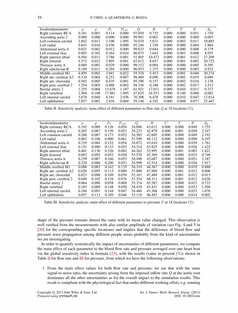
location/parameter ρ µ Pv Pext Q R C T E A0Right coronary RCA 0.181 0.003 0.114 0.000 97.059 0.735 0.000 0.000 0.051 1.750Ascending aorta 2 0.000 0.000 0.000 0.000 99.991 0.003 0.000 0.000 0.000 0.003Left common carotid 2.842 0.012 3.100 1.095 76.070 5.631 0.000 0.003 0.011 10.885Left radial 0.841 0.016 0.436 0.000 95.246 1.330 0.000 0.000 0.004 1.864Abdominal aorta A 0.021 0.002 0.012 0.000 99.633 0.044 0.000 0.000 0.008 0.179Left external iliac 0.803 0.302 0.364 0.024 86.675 3.642 0.000 0.001 0.008 8.055Right anterior tibial 6.504 0.011 3.786 0.001 51.805 10.472 0.000 0.001 0.012 27.209Right femoral 4.572 0.022 2.895 0.001 62.812 8.657 0.000 0.001 0.002 20.725Thoracic aorta A 0.069 0.001 0.029 0.000 99.312 0.094 0.000 0.000 0.005 0.395Right subclavian B 0.189 0.011 0.294 0.000 96.953 1.375 0.000 0.000 0.003 0.932Middle cerebral M1 4.859 0.002 3.041 0.022 55.518 5.453 0.000 0.001 0.046 30.274Right ant. cerebral A2 0.334 0.004 0.252 0.007 98.469 0.096 0.000 0.002 0.019 0.689Right ant. choroidal 0.503 0.005 0.435 0.001 95.296 0.157 0.000 0.002 0.016 3.138Right post. cerebral 2 1.254 0.005 0.468 0.002 94.336 0.188 0.000 0.002 0.017 3.512Basilar artery 2 1.255 0.068 13.678 1.187 61.921 17.011 0.000 0.044 0.011 0.327Right vertebral 2.504 0.108 17.981 1.095 47.625 24.553 0.000 0.140 0.006 0.082Left internal carotid 3.678 0.040 4.161 2.036 70.308 6.478 0.000 0.010 0.047 12.814Left ophthalmic 7.857 0.002 2.916 0.004 59.140 4.292 0.000 0.008 0.077 25.447
Table II. Sensitivity analysis: main effect of different parameters to flow rate Q at 18 locations (%)
location/parameter ρ µ Pv Pext Q R C T E A0Right coronary RCA 0.192 0.089 0.126 0.054 54.096 43.612 0.000 0.000 0.049 1.755Ascending aorta 2 0.265 0.087 0.150 0.053 54.223 42.879 0.000 0.001 0.058 2.247Left common carotid 0.260 0.087 0.173 0.052 54.565 42.605 0.000 0.000 0.049 2.192Left radial 0.003 0.106 0.000 0.061 51.599 48.112 0.000 0.000 0.009 0.107Abdominal aorta A 0.219 0.084 0.152 0.054 54.072 43.610 0.000 0.000 0.039 1.761Left external iliac 0.151 0.090 0.133 0.055 54.314 43.825 0.000 0.000 0.026 1.422Right anterior tibial 0.401 0.130 0.326 0.082 44.262 52.995 0.000 0.001 0.003 1.821Right femoral 0.093 0.095 0.052 0.058 53.570 45.369 0.000 0.000 0.015 0.746Thoracic aorta A 0.259 0.087 0.166 0.053 54.490 42.687 0.000 0.000 0.051 2.187Right subclavian B 0.220 0.088 0.200 0.053 54.998 42.514 0.000 0.000 0.030 1.917Middle cerebral M1 0.088 0.083 0.162 0.135 54.319 44.367 0.000 0.000 0.019 0.880Right ant. cerebral A2 0.020 0.095 0.113 0.089 51.800 47.909 0.000 0.001 0.012 0.006Right ant. choroidal 0.023 0.098 0.109 0.070 52.167 47.489 0.000 0.001 0.012 0.013Right post. cerebral 2 0.049 0.102 0.116 0.076 51.354 48.311 0.000 0.001 0.012 0.026Basilar artery 2 0.064 0.096 0.058 0.069 53.374 45.587 0.000 0.000 0.023 0.733Right vertebral 0.183 0.089 0.148 0.058 54.470 43.431 0.000 0.000 0.033 1.598Left internal carotid 0.184 0.091 0.144 0.047 54.460 43.368 0.000 0.000 0.033 1.676Left ophthalmic 0.057 0.113 0.249 0.046 53.118 46.493 0.000 0.000 0.014 0.002
Table III. Sensitivity analysis: main effect of different parameters to pressure P at 18 locations (%)
shape of the pressure remains almost the same with its mean value changed. This observation iswell verified from the measurements with also similar amplitude of variation (see Fig. 4 and 5 in[39] for the corresponding specific locations) and implies that the difference of blood flow andpressure wave propagation among different people arises probably from the kind of uncertaintieswe are investigating.
In order to quantify systemically the impact of uncertainties of different parameters, we computethe main effect of each parameter to the blood flow rate and pressure averaged over one heart beatvia the global sensitivity index in formula (23), with the results (value in percent (%)) shown inTable II for flow rate and III for pressure, from which we have the following observations:
1. From the main effect values for both flow rate and pressure, we see that with the samesignal-to-noise ratio, the uncertainty arising from the imposed inflow rate Q at the aortic rootdominates all the other uncertainties as for the overall impact to the simulation results. Thisresult is compliant with the physiological fact that under different working effort, e.g. running
Copyright c© 2013 John Wiley & Sons, Ltd. Int. J. Numer. Meth. Biomed. Engng. (2013)Prepared using cnmauth.cls DOI: 10.1002/cnm
SIMULATION-BASED UNCERTAINTY QUANTIFICATION OF HUMAN ARTERIAL NETWORK 17
0 0.1 0.2 0.3 0.4 0.5 0.6 0.7 0.80
50
G[Q
][%
]
t [s] − w.r.t.young modules E
Left common carotid
0 0.1 0.2 0.3 0.4 0.5 0.6 0.7 0.80
2
G[P
][%
]
0 0.1 0.2 0.3 0.4 0.5 0.6 0.7 0.80
1
2
3
4
5
6
7
G[Q
][%
]
t [s] − w.r.t.venous pressure Pv
Left radial
0 0.1 0.2 0.3 0.4 0.5 0.6 0.7 0.80
0.2
0.4
0.6
0.8
1
1.2
1.4
G[P
][%
]
0 0.1 0.2 0.3 0.4 0.5 0.6 0.7 0.80
100
G[Q
][%
]
t [s] − w.r.t.flow rate Q
Ascending aorta 2
0 0.1 0.2 0.3 0.4 0.5 0.6 0.7 0.8
50
G[P
][%
]
0 0.1 0.2 0.3 0.4 0.5 0.6 0.7 0.80
0.5
1
1.5
G[Q
][%
]
t [s] − w.r.t.characteristic time T
Thoracic aorta A
0 0.1 0.2 0.3 0.4 0.5 0.6 0.7 0.80
0.01
0.02
G[P
][%
]
0 0.1 0.2 0.3 0.4 0.5 0.6 0.7 0.80
5
G[Q
][%
]
t [s] − w.r.t.resistance R
Right coronary RCA
0 0.1 0.2 0.3 0.4 0.5 0.6 0.7 0.8
40 G[P
][%
]
0 0.1 0.2 0.3 0.4 0.5 0.6 0.7 0.80
0.005
0.01
G[Q
][%
]
t [s] − w.r.t.capacitance C
Abdominal aorta A
0 0.1 0.2 0.3 0.4 0.5 0.6 0.7 0.80
1
2
3x 10
−4
G[P
][%
]
0 0.1 0.2 0.3 0.4 0.5 0.6 0.7 0.80
0.1
G[Q
][%
]
t [s] − w.r.t.external pressure Pext
Left external iliac
0 0.1 0.2 0.3 0.4 0.5 0.6 0.7 0.8
0.05
G[P
][%
]
0 0.1 0.2 0.3 0.4 0.5 0.6 0.7 0.80
20
40
G[Q
][%
]
t [s] − w.r.t.reference area A0
Right anterior tibial
0 0.1 0.2 0.3 0.4 0.5 0.6 0.7 0.80
5
10
G[P
][%
]
0 0.1 0.2 0.3 0.4 0.5 0.6 0.7 0.82
3
4
5
6
7
8
9
10
G[Q
][%
]
t [s] − w.r.t.fluid density ρ
Right femoral
0 0.1 0.2 0.3 0.4 0.5 0.6 0.7 0.80
0.2
0.4
0.6
0.8
1
1.2
1.4
G[P
][%
]
0 0.1 0.2 0.3 0.4 0.5 0.6 0.7 0.80
20
G[Q
][%
]
t [s] − w.r.t.fluid viscosityµ
Right subclavian B,axillary, brachial
0 0.1 0.2 0.3 0.4 0.5 0.6 0.7 0.80
0.5
1
G[P
][%
]
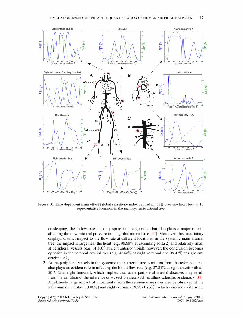
Figure 10. Time dependent main effect (global sensitivity index defined in (23)) over one heart beat at 10representative locations in the main systemic arterial tree
or sleeping, the inflow rate not only spans in a large range but also plays a major role inaffecting the flow rate and pressure in the global arterial tree [47]. Moreover, this uncertaintydisplays distinct impact to the flow rate at different locations: in the systemic main arterialtree, the impact is large near the heart (e.g. 99.99% at ascending aorta 2) and relatively smallat peripheral vessels (e.g. 51.80% at right anterior tibial); however, the conclusion becomesopposite in the cerebral arterial tree (e.g. 47.63% at right vertebral and 98.47% at right ant.cerebral A2).
2. At the peripheral vessels in the systemic main arterial tree, variation from the reference areaalso plays an evident role in affecting the blood flow rate (e.g. 27.21% at right anterior tibial,20.73% at right femoral), which implies that some peripheral arterial diseases may resultfrom the variation of the reference cross section area, such as atherosclerosis or stenosis [34].A relatively large impact of uncertainty from the reference area can also be observed at theleft common carotid (10.88%) and right coronary RCA (1.75%), which coincides with some
Copyright c© 2013 John Wiley & Sons, Ltd. Int. J. Numer. Meth. Biomed. Engng. (2013)Prepared using cnmauth.cls DOI: 10.1002/cnm

18 P. CHEN, A. QUARTERONI, G. ROZZA
pathological implications that dysfunctions of the brain (e.g. stroke) and the heart (e.g. heartattack) are due to the blockage of blood flow in the common carotid and coronary arteries [3].
3. In contrast, the variation of the inflow rate does not have so different effects on the pressureat different locations, staying between 50%− 55% for both the systemic main arterial treeand the cerebral arterial tree with an exception 44.3% (see Table III) from the most distalarterial segment right anterior tibial. In fact, most of the uncertainties display a relatively largervariation at different locations for the flow rate than for the pressure, as can be observed quiteevidently from Table II and III. It is interesting to point out that the uncertainty arising fromthe resistance at the terminal boundaries has a major impact to pressure, over 40% at all therepresentative locations. This implies that the inter-individual variability of the pressure mayarise from different structure of terminal arterial network and a more detailed modeling of thearterial network at the terminal boundaries would help to improve the simulation accuracy ofthe pressure.
4. As for the uncertainty arising from physical parameters ρ, µ, C, T,E and prescribed pressurePv, Pext, they are not so important as the parameters analyzed above for both flow rate andpressure. We remark that the analysis is under the same signal-to-noise ratio for all parameters.However, the fact is that some of the parameters are easy to measure with high accuracy inpractice , e.g. inflow rate, reference area, while some others, e.g. young modulus, are moredifficult to measure, thus they are affected by high noise potentially leading to large variationson the simulation results.
0 0.1 0.2 0.3 0.4 0.5 0.6 0.7 0.8
20
30
40
G[Q][%]
t [s] − w.r.t.reference area A0
Middle cerebral M1
0 0.1 0.2 0.3 0.4 0.5 0.6 0.7 0.80
2
4
6
G[P][%]
0 0.1 0.2 0.3 0.4 0.5 0.6 0.7 0.80
1
G[Q][%]
t [s] − w.r.t.fluid viscosityµ
Right ant. cerebral A2
0 0.1 0.2 0.3 0.4 0.5 0.6 0.7 0.80
0.5
G[P][%]
0 0.1 0.2 0.3 0.4 0.5 0.6 0.7 0.8
1
2
x 10−3
G[Q][%]
t [s] − w.r.t.external pressure Pext
Right ant. choroidal
0 0.1 0.2 0.3 0.4 0.5 0.6 0.7 0.8
0.06
0.08
G[P][%]
0 0.1 0.2 0.3 0.4 0.5 0.6 0.7 0.80
2
G[Q][%]
t [s] − w.r.t.young modules E
Right post. cerebral 2
0 0.1 0.2 0.3 0.4 0.5 0.6 0.7 0.80
1G[P][%]
0 0.1 0.2 0.3 0.4 0.5 0.6 0.7 0.80
10
20
30
40
G[Q][%]
t [s] − w.r.t.resistance R
Right vertebral
0 0.1 0.2 0.3 0.4 0.5 0.6 0.7 0.830
35
40
45
50
55
G[P][%]
0 0.1 0.2 0.3 0.4 0.5 0.6 0.7 0.8
10
15
20
G[Q][%]
t [s] − w.r.t.venous pressure Pv
Basilar artery 2
0 0.1 0.2 0.3 0.4 0.5 0.6 0.7 0.80
0.1
0.2
G[P][%]
0 0.1 0.2 0.3 0.4 0.5 0.6 0.7 0.8
50
60
70
80
G[Q][%]
t [s] − w.r.t.flow rate Q
Left internal carotid
0 0.1 0.2 0.3 0.4 0.5 0.6 0.7 0.8
45
50
55
60
G[P][%]
0 0.1 0.2 0.3 0.4 0.5 0.6 0.7 0.8
10
G[Q][%]
t [s] − w.r.t.fluid density ρ
Left ophthalmic
0 0.1 0.2 0.3 0.4 0.5 0.6 0.7 0.80
G[P][%]
Figure 11. Time dependent main effect (global sensitivity index defined in (23)) over one heart beat at 8representative locations in the cerebral arterial tree
Copyright c© 2013 John Wiley & Sons, Ltd. Int. J. Numer. Meth. Biomed. Engng. (2013)Prepared using cnmauth.cls DOI: 10.1002/cnm

SIMULATION-BASED UNCERTAINTY QUANTIFICATION OF HUMAN ARTERIAL NETWORK 19
In order to have a closer look at the sensitivity of flow rate and pressure with respect to all of theuncertainties at different time of one heart beat, we compute the variation in time of the sensitivity(time dependent main effect) of different sources of uncertainties at different locations. We pick themost important source of uncertainty in general according to Table II, e.g. imposed heart flow rateQ, at the most evident location, e.g. ascending aorta 2 (95), and then the second most importantsource at the second most evident location and so on. Following this order we plot the Figure 10and 11 for the time dependent main effect, which delivers more information about the uncertaintyimpact at different time. More specifically, we can draw the following conclusions:
1. The main effect (global sensitivity in time) of most of the parametric uncertainties varies ina large range within one heart beat. The variation of the main effect of some uncertaintiesis quite different or even opposite for flow rate and pressure in some local time region, e.g.resistance R at right coronary RCA (96) or reference area A0 at middle cerebral M1 (73),and changes in a similar way for some other uncertainties, e.g. Young modulus E at Rightpost.cerebral 2 (64) or venous pressure Pv at left radial (22). In general, even though someuncertainties dominate the others, as observed from the averaged main effect in Table II andIII, from the variation of the main effect in time we can see that quite a few uncertaintiesplay a near important role in an oscillating way. This suggests that when considering impactof uncertainty at local time, it would be misleading to overemphasize some uncertainties andneglect some others.
2. The large variation of the main effect occurs at some common time, especially at the beginningof systolic period and end of the diastolic period, e.g. flow rate Q at ascending aorta 2 (95) orcharacteristic time T at thoracic aorta A (18), or at the time of maximum or minimum flowrate during the systolic and diastolic periods, e.g. fluid density ρ at left ophthalmic (82) orfluid viscosity µ at right ant. cerebral A2 (76). Moreover, the evident main effect of most ofthe uncertainties span in a relatively large time range over one heart beat, e.g. flow rate Qat ascending aorta 2 (95) or Young modulus E at left common carotid (15), while for someother few uncertainties, it restricts at a small local time with peaks, e.g. characteristic time Tat thoracic aorta A (18) or fluid viscosity µ at right ant. cerebral A2 (76).
3.4. High dimensional parametric uncertainty - differentiated analysis
For systemic quantification of the impact of different uncertainties, it is reasonable to use the sameprobability distribution for one uncertainty in the global arterial network. However, in order toquantify some uncertainty arising from the same source but at different locations, it is more realisticto perform differentiated analysis by employing independent random variables to characterize theuncertainty at each of the location. In this section, we take two of the influential uncertainties forthe blood wave propagation (see Table III), resistance R at the 47 different distal boundaries andcross section reference areaA0 in the 103 different arterial segments of the schematic representationof the human arterial tree in Figure 3, and assign independent random variables to each of them atdifferent locations to study locally the impact of different uncertainties.
We assume that the resistance at the mth distal boundary is randomized by (13) as
Rm(ω) = exp(µe + σvYm(ω))Rm, 1 ≤ m ≤M, (26)
where Ym, 1 ≤ m ≤M are independent random variables obeying standard distribution.The largest five values of the main effect § and their total weight (in percent (%)) is shown in
Table IV and V, from which the following physiological implications can be drawn:
§We choose µe = 0.01, σv = 0.1 for the sake of computational effort and accurate evaluation of the statistics andsensitivity with small level of interpolation. By the main effect formula (23) and Smolyak sparse grid collocation method(17) with the first level of interpolation q −K = 1, we compute main sensitivity at the 18 representative locations withrespect to each random resistance at the 47 distal boundaries.
Copyright c© 2013 John Wiley & Sons, Ltd. Int. J. Numer. Meth. Biomed. Engng. (2013)Prepared using cnmauth.cls DOI: 10.1002/cnm

20 P. CHEN, A. QUARTERONI, G. ROZZA
1. In general, the largest impact to flow rate comes from the uncertainty of resistance at thenearest distal boundaries and it dominates the impact of resistance variation from all the otherboundaries, e.g. the impact to right anterior tibial (92.14%) comes from its distal boundary.
2. In particular, the largest impact of the uncertainty of resistance to flow rate at the ascendingaorta 2 comes from the coronary arteries (99, 98, 96), which implies that strong resistance oreven blockage of the coronary arteries would potentially lead to heart attack or heart failureas expected.
3. As for the impact to pressure, the largest values come mostly from the uncertainty of resistanceat the distal boundaries of abdominal aorta branches along the ascending aorta (34, 36, 38,33), no matter where the location of the pressure is considered. This indicates that resistanceat these locations have a major influence to the global pressure and a more detailed modelingof the branch arteries is needed to improve the simulation precision.
location/order 1st 2nd 3rd 4th 5th 1-5Right coronary RCA 98.010 (96) 0.579 (34) 0.385 (36) 0.383 (38) 0.288 (26) 99.645Ascending aorta 2 33.864 (99) 22.409 (98) 20.864 (96) 6.975 (34) 4.649 (36) 88.762Left common carotid 16.781 (34) 11.166 (36) 11.142 (38) 9.760 (78) 8.225 (26) 57.074Left radial 96.782 (22) 0.923 (34) 0.613 (36) 0.612 (38) 0.459 (26) 99.389Abdominal aorta A 35.757 (34) 23.834 (36) 23.802 (38) 6.727 (26) 2.027 (33) 92.147Left external iliac 64.780 (47) 14.886 (48) 4.873 (34) 4.369 (49) 3.291 (38) 92.198Right anterior tibial 92.143 (55) 2.066 (34) 1.403 (38) 1.395 (36) 1.044 (54) 98.051Right femoral 65.185 (54) 19.086 (55) 4.749 (34) 3.213 (38) 3.200 (36) 95.434Thoracic aorta A 28.948 (34) 19.304 (36) 19.281 (38) 13.910 (26) 4.030 (33) 85.472Right subclavian B 47.514 (8) 38.477 (11) 4.160 (34) 2.767 (36) 2.761 (38) 95.680Middle cerebral M1 45.862 (75) 44.636 (74) 2.839 (34) 1.886 (36) 1.881 (38) 97.103Right ant. cerebral A2 98.004 (76) 0.569 (34) 0.378 (36) 0.377 (38) 0.283 (26) 99.610Right ant. choroidal 97.686 (100) 0.670 (34) 0.445 (36) 0.443 (38) 0.334 (26) 99.577Right post. cerebral 2 97.666 (64) 0.670 (34) 0.445 (36) 0.444 (38) 0.334 (26) 99.560Basilar artery 2 34.116 (65) 34.053 (64) 12.039 (58) 12.039 (57) 1.273 (34) 93.520Right vertebral 34.364 (65) 34.298 (64) 12.124 (58) 12.124 (57) 1.166 (78) 94.075Left internal carotid 23.796 (78) 10.593 (102) 10.019 (34) 8.436 (75) 8.303 (76) 61.147Left ophthalmic 95.852 (82) 1.232 (34) 0.819 (36) 0.817 (38) 0.615 (26) 99.336
Table IV. The largest five values and their summation of main effect (value in percent (%)) of flow rate withrespect to resistance from their corresponding boundaries in bracket (·) at 18 locations
location/order 1st 2nd 3rd 4th 5th 1-5Right coronary RCA 29.782 (34) 19.783 (36) 19.725 (38) 14.823 (26) 4.135 (33) 88.248Ascending aorta 2 30.395 (34) 20.190 (36) 20.131 (38) 15.127 (26) 4.219 (33) 90.063Left common carotid 30.390 (34) 20.186 (36) 20.127 (38) 15.129 (26) 4.219 (33) 90.051Left radial 24.430 (22) 22.267 (34) 14.790 (36) 14.747 (38) 11.115 (26) 87.350Abdominal aorta A 30.959 (34) 20.557 (36) 20.491 (38) 14.091 (26) 4.251 (33) 90.350Left external iliac 30.371 (34) 20.597 (38) 20.478 (36) 13.650 (26) 4.133 (33) 89.229Right anterior tibial 53.200 (55) 12.236 (34) 8.317 (38) 8.264 (36) 6.540 (54) 88.556Right femoral 29.180 (34) 19.806 (38) 19.688 (36) 13.052 (26) 3.972 (33) 85.698Thoracic aorta A 30.403 (34) 20.194 (36) 20.134 (38) 15.138 (26) 4.221 (33) 90.091Right subclavian B 30.117 (34) 20.007 (36) 19.952 (38) 14.996 (26) 4.179 (33) 89.252Middle cerebral M1 29.744 (34) 19.757 (36) 19.699 (38) 14.814 (26) 4.129 (33) 88.143Right ant. cerebral A2 24.067 (76) 22.659 (34) 15.050 (36) 15.005 (38) 11.286 (26) 88.067Right ant. choroidal 23.451 (34) 21.853 (100) 15.578 (36) 15.532 (38) 11.681 (26) 88.094Right post. cerebral 2 27.227 (64) 21.695 (34) 14.411 (36) 14.369 (38) 10.805 (26) 88.506Basilar artery 2 29.461 (34) 19.569 (36) 19.512 (38) 14.668 (26) 4.090 (33) 87.300Right vertebral 30.179 (34) 20.047 (36) 19.989 (38) 15.023 (26) 4.190 (33) 89.429Left internal carotid 30.228 (34) 20.079 (36) 20.020 (38) 15.053 (26) 4.197 (33) 89.576Left ophthalmic 24.635 (34) 17.590 (82) 16.356 (36) 16.308 (38) 12.280 (26) 87.168
Table V. The largest five values and their summation of main effect (value in percent (%)) of pressure withrespect to resistance from their corresponding boundaries in bracket (·) at 18 locations
Copyright c© 2013 John Wiley & Sons, Ltd. Int. J. Numer. Meth. Biomed. Engng. (2013)Prepared using cnmauth.cls DOI: 10.1002/cnm

SIMULATION-BASED UNCERTAINTY QUANTIFICATION OF HUMAN ARTERIAL NETWORK 21
As for the uncertainty quantification with respect to reference areaA0, we take the same numericaldesign as for the resistance, leading to 103 independent random variables. The main effect resultsare shown in Table VI for flow rate and VII for pressure, from which we may have the followingobservations:
1. In general, the most important uncertainty for the flow rate at the representative locationscomes from the location itself or the few nearest arterial segments. For instance, the maineffect with the largest value 98.5% at left ophthalmic (82) in the cerebral arterial tree is due tothe uncertainty of the reference area of the arterial segment itself.
2. The largest values of the main effect for the pressure concentrate again at the few locations(27, 95, 18), which are very close to the heart, i.e. a small change of the cross sectionarea of the large arteries near the heart leads to relatively large variation of pressure wavepropagation in the global arterial network, which implies that some arterial diseases suchas aorta atherosclerosis or the equivalent aorta stiffening may result in severe change of theglobal blood pressure.
3. An interesting observation is that the main effect of the flow rate at the abdominal aorta A(28) distributes rather dispersedly than concentrated in a small region, i.e. coming from theuncertainty of the reference area not only near the heart (ascending aorta 2 (95)) but alsofrom the four longest peripheral arterial segments - the arms (7, 21) and legs (52, 46) as wellas other regions. These many influential sources might provide an environment to developaneurysms with high probability, which could also be observed in the basilar artery 2 (56),see Table VI.
location/order 1st 2nd 3rd 4th 5th 1-5Right coronary RCA 45.498 (96) 13.333 (27) 9.516 (95) 4.743 (18) 4.091 (21) 77.181Ascending aorta 2 77.616 (95) 7.039 (1) 5.138 (98) 1.907 (27) 1.225 (46) 92.925Left common carotid 58.289 (16) 10.457 (12) 7.408 (15) 3.479 (69) 3.311 (68) 82.943Left radial 89.126 (22) 2.912 (21) 2.443 (27) 1.362 (95) 0.994 (7) 96.837Abdominal aorta A 15.811 (95) 10.886 (7) 10.786 (21) 8.570 (52) 8.570 (46) 54.623Left external iliac 46.320 (46) 22.054 (49) 19.212 (48) 4.457 (44) 1.769 (47) 93.811Right anterior tibial 92.292 (55) 6.218 (52) 0.329 (54) 0.318 (95) 0.181 (7) 99.338Right femoral 33.939 (55) 32.890 (52) 29.903 (54) 0.629 (7) 0.566 (95) 97.927Thoracic aorta A 25.131 (95) 13.627 (21) 12.261 (7) 8.885 (14) 4.138 (15) 64.042Right subclavian B 32.805 (11) 29.928 (7) 26.728 (8) 2.912 (21) 1.692 (27) 94.065Middle cerebral M1 48.828 (74) 48.447 (75) 0.820 (16) 0.479 (27) 0.325 (95) 98.898Right ant. cerebral A2 75.245 (76) 4.403 (27) 3.530 (12) 3.005 (95) 2.095 (68) 88.277Right ant. choroidal 91.213 (100) 2.504 (12) 1.562 (27) 1.069 (95) 0.604 (9) 96.953Right post. cerebral 2 91.862 (64) 1.878 (27) 1.287 (95) 0.743 (21) 0.670 (18) 96.441Basilar artery 2 27.970 (9) 18.040 (20) 15.745 (16) 15.338 (6) 15.088 (12) 92.181Right vertebral 63.532 (6) 19.705 (20) 6.048 (9) 3.454 (16) 3.319 (12) 96.058Left internal carotid 62.295 (16) 11.773 (12) 4.017 (69) 3.794 (68) 3.604 (74) 85.483Left ophthalmic 98.458 (82) 0.491 (16) 0.267 (27) 0.180 (95) 0.096 (9) 99.492
Table VI. The largest five values and their summation of main effect (value in percent (%)) of flow rate withrespect to reference area from their corresponding boundaries in bracket (·) at 18 locations
4. CONCLUDING REMARKS
In this work we presented a general framework for simulation-based uncertainty quantification inthe human arterial network. We identified the main uncertainties arising from various sources andcharacterized them by random variables obeying certain specific probability distributions. Based ona one dimensional deterministic fluid structure interaction model (a system of nonlinear hyperbolicequation), we introduced the stochastic model by incorporating many different kinds of uncertaintiesinto blood flow in arteries and its interaction with arterial walls in a human arterial network.
Copyright c© 2013 John Wiley & Sons, Ltd. Int. J. Numer. Meth. Biomed. Engng. (2013)Prepared using cnmauth.cls DOI: 10.1002/cnm
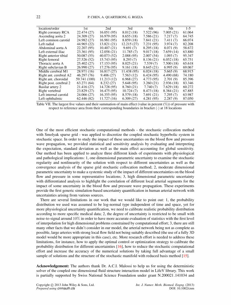
22 P. CHEN, A. QUARTERONI, G. ROZZA
location/order 1st 2nd 3rd 4th 5th 1-5Right coronary RCA 22.474 (27) 16.051 (95) 8.012 (18) 7.522 (96) 7.005 (21) 61.064Ascending aorta 2 24.309 (27) 16.979 (95) 8.655 (18) 7.586 (21) 7.217 (7) 64.745Left common carotid 24.982 (27) 16.981 (95) 8.859 (18) 7.841 (21) 7.411 (7) 66.074Left radial 44.965 (22) 13.821 (21) 12.215 (27) 7.231 (95) 3.974 (7) 82.208Abdominal aorta A 22.207 (95) 10.407 (21) 9.691 (7) 8.295 (18) 8.071 (9) 58.672Left external iliac 23.361 (95) 12.058 (21) 11.785 (7) 9.017 (18) 7.659 (14) 63.880Right anterior tibial 50.087 (55) 40.073 (52) 2.088 (95) 2.007 (54) 1.093 (7) 95.347Right femoral 27.526 (52) 15.743 (95) 8.293 (7) 8.136 (21) 6.052 (18) 65.751Thoracic aorta A 25.402 (27) 17.153 (95) 8.025 (21) 7.539 (7) 7.500 (18) 65.618Right subclavian B 26.990 (27) 17.276 (95) 9.161 (18) 8.645 (21) 6.995 (9) 69.067Middle cerebral M1 28.971 (16) 16.817 (27) 11.438 (95) 6.024 (18) 5.665 (9) 68.915Right ant. cerebral A2 46.297 (76) 9.406 (27) 7.563 (12) 6.424 (95) 4.490 (68) 74.180Right ant. choroidal 59.741 (100) 11.213 (12) 6.968 (27) 4.773 (95) 2.701 (9) 85.396Right post. cerebral 2 63.271 (64) 8.232 (27) 5.648 (95) 3.260 (21) 2.936 (18) 83.346Basilar artery 2 21.416 (27) 14.728 (95) 8.760 (21) 7.740 (7) 7.629 (18) 60.272Right vertebral 23.829 (27) 16.475 (95) 10.724 (7) 8.473 (18) 8.384 (21) 67.885Left internal carotid 24.066 (27) 16.355 (95) 8.579 (18) 7.691 (21) 7.295 (7) 63.987Left ophthalmic 62.446 (82) 11.727 (16) 6.309 (27) 4.281 (95) 2.287 (9) 87.050
Table VII. The largest five values and their summation of main effect (value in percent (%)) of pressure withrespect to reference area from their corresponding boundaries in bracket (·) at 18 locations
One of the most efficient stochastic computational methods - the stochastic collocation methodwith Smolyak sparse grid - was applied to discretize the coupled stochastic hyperbolic system instochastic space. In order to study the impact of these uncertainties on the blood flow and pressurewave propagation, we provided statistical and sensitivity analysis by evaluating and interpretingthe expectation, standard deviation as well as the main effect accounting for global sensitivity.Our method has been applied to analyze three different kinds of experiments with physiologicaland pathological implications: 1, one dimensional parametric uncertainty to examine the stochasticregularity and nonlinearity of the solution with respect to different uncertainties as well as theconvergence analysis of the sparse grid stochastic collocation method; 2, moderate dimensionalparametric uncertainty to make a systemic study of the impact of different uncertainties on the bloodflow and pressure in some representative locations; 3, high dimensional parametric uncertaintywith differentiated analysis to highlight the correlation of different local arterial segments for theimpact of some uncertainty in the blood flow and pressure wave propagation. These experimentsprovide the first generic simulation-based uncertainty quantification in human arterial network withuncertainties arising from various sources.
There are several limitations in our work that we would like to point out: 1, the probabilitydistribution we used was assumed to be log-normal type independent of time and space, yet formore physiological uncertainty quantification, we need to calibrate realistic probability distributionaccording to more specific medical data; 2, the degree of uncertainty is restricted to be small withnoise-to-signal around 10% in order to have more accurate evaluation of statistics with the first levelof interpolation for high dimensional problems constrained by computational effort; 3, there are stillmany other facts that we didn’t consider in our model, the arterial network being not as complete aspossible, large arteries with strong local flow field not being suitably described (the use of a fully 3Dmodel would be more appropriate in this case), etc. More research effort is needed to address theselimitations, for instance, how to apply the optimal control or optimization strategy to calibrate theprobability distribution for different uncertainties [16], how to reduce the stochastic computationaleffort and increase the accuracy of the numerical solutions by taking full advantage of a smallsample of solutions and the structure of the stochastic manifold with reduced basis method [15].
Acknowledgement: The authors thank Dr. A.C.I. Malossi to help us for using the deterministicsolver of the coupled one dimensional fluid structure interaction model in LifeV library. This workis partially supported by Swiss National Science Foundation under grant N.200021 141034 and
Copyright c© 2013 John Wiley & Sons, Ltd. Int. J. Numer. Meth. Biomed. Engng. (2013)Prepared using cnmauth.cls DOI: 10.1002/cnm

SIMULATION-BASED UNCERTAINTY QUANTIFICATION OF HUMAN ARTERIAL NETWORK 23
the MATHCARD project ERC-2008-AdG-227058 http://www.mathcard.eu/. G. Rozzaacknowledges the excellence grant NOFYSAS of SISSA.
REFERENCES
1. LifeV Project, http://www.lifev.org/.2. D. Ambrosi, A. Quarteroni, and G. Rozza. Modelling of Physiological Flows. Springer, Series MS&A, 2011.3. American Heart Association. Heart and stroke facts. The Association, 1991.4. I. Babuska, F. Nobile, and R. Tempone. A stochastic collocation method for elliptic partial differential equations
with random input data. SIAM Journal on Numerical Analysis, 45(3):1005–1034, 2007.5. I. Babuska, F. Nobile, and R. Tempone. Reliability of computational science. Numerical Methods for Partial
Differential Equations, 23(4):753–784, 2007.6. I. Babuska, F. Nobile, and R. Tempone. A stochastic collocation method for elliptic partial differential equations
with random input data. SIAM review, 52(3):317, 2010.7. I. Babuska, R. Tempone, and G.E. Zouraris. Galerkin finite element approximations of stochastic elliptic partial
differential equations. SIAM Journal on Numerical Analysis, 42(2):800–825, 2005.8. S. Badia, A. Quaini, and A. Quarteroni. Modular vs. non-modular preconditioners for fluid–structure systems with
large added-mass effect. Computer Methods in Applied Mechanics and Engineering, 197(49):4216–4232, 2008.9. S. Badia, A. Quaini, and A. Quarteroni. Splitting methods based on algebraic factorization for fluid-structure
interaction. SIAM Journal on Scientific Computing, 30(4):1778–1805, 2008.10. S. Boyaval, C. Le Bris, T. Lelievre, Y. Maday, N.C. Nguyen, and A.T. Patera. Reduced basis techniques for
stochastic problems. Archives of Computational Methods in Engineering, 17:435–454, 2010.11. J.T. Bushberg. The essential physics of medical imaging. Williams & Wilkins, 2002.12. G.T. Buzzard and D. Xiu. Variance-based global sensitivity analysis via sparse-grid interpolation and cubature.
Communications in Computational Physics, 9:542–67, 2011.13. C. Canuto, MY Hussaini, A. Quarteroni, and TA Zang. Spectral Methods: Fundamentals in Single Domains.
Springer, 2006.14. D. Chapelle, M. Fernandez, J.F. Gerbeau, P. Moireau, J. Sainte-Marie, and N. Zemzemi. Numerical simulation of
the electromechanical activity of the heart. Functional Imaging and Modeling of the Heart, 5528:357–365, 2009.15. P. Chen, A. Quarteroni, and G. Rozza. Comparison of reduced basis method and collocation method for stochastic
elliptic problems. EPFL, MATHICSE Report 34, submitted, 2012.16. P. Chen, A. Quarteroni, and G. Rozza. Stochastic optimal Robin boundary control problems of advection-
dominated elliptic equations. EPFL, MATHICSE Report 23, submitted, 2012.17. P. Crosetto, S. Deparis, G. Fourestey, and A. Quarteroni. Parallel algorithms for fluid-structure interaction problems
in haemodynamics. SIAM Journal on Scientific Computing, 33(4):1598–1622, 2011.18. C. D’Angelo and A. Quarteroni. On the coupling of 1d and 3d diffusion-reaction equations. application to tissue
perfusion problems. Mathematical Models and Methods in Applied Sciences, 18(8):1481–1504, 2008.19. A.C. Davison. Statistical models. Cambridge University Press, 2003.20. S. Deparis, M. Discacciati, G. Fourestey, and A. Quarteroni. Fluid-structure algorithms based on steklov-poincare
operators. Computer Methods in Applied Mechanics and Engineering, 195(41-43):5797–5812, 2006.21. G.S. Fishman. Monte Carlo: Concepts, Algorithms, and Applications. Springer, 1996.22. L. Formaggia, D. Lamponi, and A. Quarteroni. One-dimensional models for blood flow in arteries. Journal of
engineering mathematics, 47(3):251–276, 2003.23. L. Formaggia, A. Quarteroni, and A. Veneziani. Cardiovascular Mathematics: Modeling and simulation of the
circulatory system, volume 1. Springer, 2009.24. L. Grinberg, T. Anor, JR Madsen, A. Yakhot, and GE Karniadakis. Large-scale simulation of the human arterial
tree. Clinical and Experimental Pharmacology and Physiology, 36(2):194–205, 2009.25. A. Klimke. Uncertainty modeling using fuzzy arithmetic and sparse grids. Universitat Stuttgart. PhD thesis,
Universitat Stuttgart, 2006.26. D. Kressner and C. Tobler. Low-rank tensor Krylov subspace methods for parametrized linear systems. SIAM
Journal on Matrix Analysis and Applications, 32(4):1288–1316, 2011.27. T. Lassila, A. Manzoni, A. Quarteroni, and G. Rozza. A reduced computational and geometrical framework for
inverse problems in haemodynamics. MATHICSE Report 12, 2011.28. A.C.I. Malossi. Partitioned Solution of Geometrical Multiscale Problems for the Cardiovascular System. PhD
thesis, 2012.29. A.C.I. Malossi, P.J. Blanco, and S. Deparis. A two-level time step technique for the partitioned solution of one-
dimensional arterial networks. Computer Methods in Applied Mechanics and Engineering, 237-240(0):212–226,2012.
30. F. Nobile. Coupling strategies for the numerical simulation of blood flow in deformable arteries by 3d and 1dmodels. Mathematical and Computer Modelling, 49(11-12):2152–2160, 2009.
31. F. Nobile, R. Tempone, and C.G. Webster. An anisotropic sparse grid stochastic collocation method for partialdifferential equations with random input data. SIAM Journal on Numerical Analysis, 46(5):2411–2442, 2008.
32. F. Nobile, R. Tempone, and C.G. Webster. A sparse grid stochastic collocation method for partial differentialequations with random input data. SIAM Journal on Numerical Analysis, 46(5):2309–2345, 2008.
33. A. Nouy. A generalized spectral decomposition technique to solve a class of linear stochastic partial differentialequations. Computer Methods in Applied Mechanics and Engineering, 196(45-48):4521–4537, 2007.
34. K. Ouriel. Peripheral arterial disease. The lancet, 358(9289):1257–1264, 2001.35. A. Quaini and A. Quarteroni. A semi-implicit approach for fluid-structure interaction based on an algebraic
fractional step method. Mathematical models and methods in applied sciences, 17(06):957–983, 2007.
Copyright c© 2013 John Wiley & Sons, Ltd. Int. J. Numer. Meth. Biomed. Engng. (2013)Prepared using cnmauth.cls DOI: 10.1002/cnm

24 P. CHEN, A. QUARTERONI, G. ROZZA
36. A. Quarteroni and L. Formaggia. Mathematical modelling and numerical simulation of the cardiovascular system.Handbook of numerical analysis, 12:3–127, 2004.
37. A. Quarteroni, R. Sacco, and F. Saleri. Numerical Mathematics. Springer, 2007.38. A. Quarteroni, M. Tuveri, and A. Veneziani. Computational vascular fluid dynamics: problems, models and
methods. Computing and Visualization in Science, MS&A Series, 2(4):163–197, 2000.39. P. Reymond, F. Merenda, F. Perren, D. Rufenacht, and N. Stergiopulos. Validation of a one-dimensional model of
the systemic arterial tree. American Journal of Physiology-Heart and Circulatory Physiology, 297(1):H208–H222,2009.
40. G. Rozza. Shape design by optimal flow control and reduced basis techniques: Applications to bypassconfigurations in haemodynamics. PhD thesis, EPFL, 2005.
41. A. Saltelli, K. Chan, E.M. Scott, et al. Sensitivity analysis, volume 134. Wiley New York, 2000.42. A. Saltelli, M. Ratto, T. Andres, F. Campolongo, J. Cariboni, D. Gatelli, M. Saisana, and S. Tarantola. Global
sensitivity analysis: the primer. Wiley Online Library, 2008.43. S. Sankaran and A.L. Marsden. A stochastic collocation method for uncertainty quantification and propagation in
cardiovascular simulations. Journal of Biomechanical Engineering, 133(31):228–240, 2011.44. S.J. Sherwin, L. Formaggia, J. Peiro, and V. Franke. Computational modelling of 1d blood flow with variable
mechanical properties and its application to the simulation of wave propagation in the human arterial system.International Journal for Numerical Methods in Fluids, 43(6-7):673–700, 2003.
45. S.A. Smolyak. Quadrature and interpolation formulas for tensor products of certain classes of functions. InDoklady Akademii Nauk SSSR, volume 4, pages 240–243, 1963.
46. C. Soize. Construction of probability distributions in high dimension using the maximum entropy principle:Applications to stochastic processes, random fields and random matrices. International Journal for NumericalMethods in Engineering, 76(10):1583–1611, 2008.
47. N. Westerhof, N. Stergiopulos, and M. Noble. Snapshots of hemodynamics: an aid for clinical research andgraduate education. Springer, 2010.
48. D. Xiu and J.S. Hesthaven. High-order collocation methods for differential equations with random inputs. SIAMJournal on Scientific Computing, 27(3):1118–1139, 2005.
49. D. Xiu and S.J. Sherwin. Parametric uncertainty analysis of pulse wave propagation in a model of a human arterialnetwork. Journal of Computational Physics, 226(2):1385–1407, 2007.
50. P. Zunino. Mathematical and numerical modeling of mass transfer in the vascular system. PhD thesis, EPFL,2002.
Copyright c© 2013 John Wiley & Sons, Ltd. Int. J. Numer. Meth. Biomed. Engng. (2013)Prepared using cnmauth.cls DOI: 10.1002/cnm