simulation modeling applications in organization management shweikeh_0.pdf · simulation modeling...

An-Najah National University

Faculty of Graduate Studies

Simulation Modeling Applications in Organization

Management

By

Ahmed Adli Shwaikeh

Supervisor

Dr. Amjed Ghanim

This Thesis is submitted in Partial Fulfillment of the Requirements for

the Degree of Master of Engineering Management, Faculty of

Graduate Studies, An-Najah National University, Nablus- Palestine.

2013

II

Simulation Modeling Applications In Organization

Management

By

Ahmed Adli Shwaikeh

This Thesis was defended successfully on 4/4/2013 and approved by:

Defense Committee Members Signatures

Dr. Amjed Ghanim (Supervisor) .………………

Dr. Mahasen Anabtawi (External Examiner) ……………......

Dr. Yahya Saleh (Internal Examiner) ..………………

III

ACKNOWLEDGMENT

In the beginning I thank ALLAH and praise Him in a manner that befits the

(infinite) number of His creation, and as it pleases Him, for supporting me

in the completion of this work. I would like to express my gratitude to my

supervisor Dr. Amjed Ghanim for being an outstanding advisor and

excellent professor. I am deeply indebted to my committee members, Dr.

Mahasen Anabtawi and Dr. Yahya Saleh for their time and effort in

reviewing this work.

I am greatly indebted to Sinokrot Global Group for their business case

contributions. I’m especially indebted to G.M Mazen Sinokrot, Eng.

Muhsen Sinokrot, Eng. Hamzeh Sinokrot and the staff who shared their

experiences and insights with me.

My sincere thanks go to Dr. Husam Araman and Dr. Mohamed Othman for

providing me with their valuable insights on my research progress.

I am deeply and forever indebted to my parents Adli and Basemah for their

love, support and encouragement throughout my entire life. I am also very

grateful to my brothers; Eng. Hussein, Mr. Tariq, Mr. Oday, Dr. Abdul

Aziz, sister Haneen, and to their lovely families.

Words fail me to express my appreciation to my wife Dr. Heba whose

dedication, love and persistent confidence in me, have taken the load off

my shoulder. I owe her for being unselfishly letting her intelligence,

passions, and ambitions collide with mine.

iv

االقرار

:أنا الموقع أدناه مقدم الرسالة التي تحمل العنوان

Simulation Modeling Applications In Organization

Management

Declaration

The work provided in this thesis, unless otherwise referenced, is the

researcher's own work, and has not been submitted elsewhere for any other

degree or qualification.

Student's Name: اسم الطالب :

Signature: : التوقيع

Date: : التاريخ

v

LIST OF CONTENTS No. Subject Page

SIGNATURES II

ACKNOWLEDGMENT III

DECLARATION IV

LIST OF FIGURS VIII

LIST OF TABLES X

ABSTRACT XII

CHAPTER 1: INTRODUCTION 1

1.1 SIMULATION 2

1.2 STRATEGIC MANAGEMENT AND SIMULATION 2

1.3 RESEARCH STATMENT 4

1.4 RESEARCH OBJECTIVES 6

1.5 RESEARCH (IMPORTANCE) 6

1.6 METHODOLOGY 7

1.7 RESEARCH TOOLS 7

1.8 ORGANIZATION OF THE THISES 8

CHAPTER 2: SIMULATION 10

2.1 SYSTEM, MODEL, AND SIMULATION 10

2.1.1 SYSTEM 10

2.1.2 MODEL 11

2.1.3 SIMULATION 12

2.2 TYPES OF SIMULATION 13

2.3 ROLE OF SIMULATION 15

2.4 SIMULATION ADVANTAGES 17

2.5 DISADVATAGES OF SIMULATION 20

2.6 WHEN SIMULATION IS APPROPRIATE 21

2.7 SIMULATION METHODOLOGY 21

2.7.1 STEP 1: DEFINING OBJECTIVE, SCOPE, AND

REQUIREMENTS

22

2.7.2 STEP 2: COLLECTING AND ANALYZING SYSTEM

DATA

23

2.7.3 STEP 3: BUILDING THE MODEL 24

2.7.4 STEP 4: VERIFYING AND VALIDATING THE MODEL 24

2.7.5 STEP 5: CONDUCTING SIMULATION EXPERIMENTS 25

2.7.6 STEP 6: PRESENT THE RESULTS 25

CHAPTER 3: LITER ATURE REVIEW 27

3.1 SUPPLY CAHIN 27

3.2 INVENTORY MANAGMNET 30

3.3 MANUFACTURING MANAGMENT 31

vi

3.4 RISK MANAGEMENT 37

CHAPTER 4: CASE STUDY 39

4.1 SINOKROT FOOD COMPANY 39

4.2 SINOKROT SYSTEM 40

4.2.1 PRODUCTION 40

4.2.2 RAW MATERIALS INVENTORY MANAGEMENT 43

4.2.3 DISTRIBUTION CENTERS AND PRODUCT DEMAND 45

4.2.4 SALES INVENTORY MANAGEMENT 46

4.2.5 SALES, PALLETIZING AND TRANSPORTATION 48

4.2.6 GENERAL CONCEPTUAL MODEL 49

4.3 PROBLEM DIFINITION AND OBJECTIVES 49

4.4 SIMULATION MODEL AND DESCRIPTION 51

4.5. MODEL VERIFICATION 69

4.5.1 DIVIDE AND CONQURE APPROACH 69

4.5.2 ANIMATION 69

4.6 MODEL VALIDATION 73

4.7 REPLICATION EXPERIMENTALDESIGN 78

4.8 SCENARIOS DEVELOPMENT AND ANALYSIS 79

4.8.1 SCENARIO 1: 15% MARKET DEMAND INCREASE 79

4.8.2 SCENARIO 2: DEVELOPMENT OF SALES INVENTORY

TARGET LEVEL

84

4.8.3 SCENARIO 3: ALLOCTING PRODCUTION LINE 1 FOR

PRODUCT GROUP 1 ONLY

88

4.8.4 SCENARIO 4: RAW MATERIAL INVENTORY

MANGMENT BASED ON FIXED-ORDERED

QUANTITY

90

4.8.5 SCENARIO 5: RAW MATERIAL INVENTORY

MANGMENT BASED ON FIXED-TIME PERIOD MODEL

104

CHAPTER 5: THESIS CONCLUSION 114

5.1 THESIS RESULTS AND CONCLUSIONS 114

5.2 CONTRIBUTION TO KNOWLEDG AND PRACTICE 116

5.3 THESIS RECOMANDATIONS AND FUTURE WORKS 118

BIOGRAPHY 121

APPENDICES 128

APPENDIX A: CONCEPTUAL MODEL 128

APPENDIX B: INPUT DATA FITTING (SAMPLES) 137

GENERAL CONCEPTOF INPUT DATA FITTING 137

APPENDIX C: SINOKROT SIMULATION MODEL 144

APPENDIX D: SIMULATION MODEL VALIDATION 153

1-DEMAND VALIDATION 153

vii

2-PRODUCTION RATE VALIDATION 157

3. PRODUCED QUANTITIES VALIDATION 164

APPENDIX E: SIMULATIOM SCENARIOS 168

SCENARIO 4: OPTIMUM RE-0RDER POINT 170

SCENARIO 5: OPTIMUM FIXED- TIME INVENTORY

REVIEW

175

viii

LIST OF FIGURS Figure

No.

Subject Page

(1.1) MCDM and strategic, tactical, operational levels 5

(2.1) Elements of a system from simulation prospective 13

(2.2) Iterative nature of simulation 22

(4.1) General Sinokrot conceptual mode 50

(4.2) Create entities and orders (main Sinokrot model) 54

(4.4) Sub-Model: Production Management (Continue) 61

(4.5) Raw Material order 64

(4.6) Create entities and orders 66

(4.7) Delivery management 67

(4.8) Distribution management 68

(4.9) Simulation model structure for verification 70

(4.10) Simulation entity type and picture for verification 70

(4.11) Following the entities for verification 72

(4.12) Using variable displays for verification 73

(4.13) Check the simulation model for verification 73

(4.14) Simulation model validation procedure 76

(4.15) Statistical steady state sales versus number of

simulation replications

76

(4.16) Annual Product cost, based on size of order 79

(4.17) Inventory position and lead time lead time are

stochastic (fixed order quantity)

92

(4.20) Proposed simulation model of fixed time based raw

material inventory

106

(4.21) Raw material simulation model in case of stochastic

demand and stochastic lead time

107

(4.22) Raw Material 4 Inventory for main Sinokrot and

scenario 5 model

113

B.1 StatFit software fitting results 139

B.2 Daily demand StatFit software fitting results 141

B.3 Daily demand StatFit software fitting results 142

C.1 Main Sinokrot simulation model 144

C.2 Simulation modules 144

ix

C.3 Structure of main Sinokrot simulation model 145

C.4 Distribution centers demand and sales inventory 145

C.5 Distribution centers demand sub-model 146

C.6 Sales inventory sub-model 146

C.7 Production management and production 147

C.8 Production management sub-model 147

C.9 Raw material requirement planning sub-model 148

C.10 Production sub-model 148

C.11 Break-down sub-model 149

C.12 Raw material inventory sub-model 149

C.13 Raw material orders 150

C.14 Structure of Sinokrot sales delivery simulation

model

151

C.15 Delivery orders 152

C.16 Distribution orders 152

E.1 Scenario 4:Q-based inventory in case of stochastic

demand and stochastic lead time

170

E.2 Scenario 5:Inventory fixed-time reviewing in case

of stochastic demand and stochastic lead time

175

x

LIST OF TABLES Table

No.

Subject Page

(1.1) Thesis Time Frame 7

(3.1) Supply chain planning issues 29

(4.1) Used ARENA terms and abbreviations 52

(4.2) Simulation entities and orders sequence 53

(4.3) Simulation entity type and picture 71

(4.4) Simulation model validation summary (continue) 77

(4.5) Scenario1 comparisons (15% demand increase),

(continue)

82

(4.6) Production line utilization 83

(4.7) Scenario 2 comparison (Development of sales

inventory target level)

86

(4.8) Sales inventory average reduction 87

(4.9) Scenario 3 comparison 89

(4.10) Annual production line utilization 89

(4.11) Ad hoc raw material inventory system, continue 94

(4.11) Ad hoc raw material inventory system 94

(4.12) Scenario 4 (Q-based inventory system 94

(4.13) Compared costs of scenario 4 with ad hoc system 101

(4.14) Scenario 5 (T-based inventory system) 110

(4.15) Compared total inventory costs (scenario 5) with

Ad hoc system

112

(A.1) Production lines and product groups 128

(A.2) Production Lines rates 128

(A.3) General Production Line Breakdown 129

(A.4) Raw Material Order Frequency, Ordered Quantities

and Reorder Point

129

(A.5) Bill of Materials 130

(A.6) Daily product demand statistical distributions 131

(A.7) Daily product demand of distribution center

percentage

135

(A.8) Product Sales Target Level 135

(A.9) Number of cases per pallet 136

xi

(B.3) Daily demand StatFit software fitting results 137

(D.1) Real demand (semi-month demand of some

products)

153

(D.2) Simulation model demand (semi-month demand of

some products)

154

(D.3) Paired T-Test (Demand) 155

(D.4) Non-parametric test (rank sum test) (Demand) 155

(D.5) Demand validation summery 156

(D.6) Real Production rate (production rate of some

products)

158

(D.7) Paired T-Test (Production rate) 161

(D.8) Nonparametric test 162

(D.9) Production rate validation summery 163

(D.10) Real produced quantities of some products 164

(D.11) Simulation produced quantities of some products 165

(D.12) Paired T-Test (produced quantities of some

products)

166

(D.13) Nonparametric test 166

(D.14) Demand validation summery 167

(E.1) Sales T-test and F-test results (scenario 1) 168

(E.2) Fixed Q-based raw material inventory (scenario 4) 171

(E.3) Raw material inventory level T-test and F-test

results (ad hoc and scenario 4 models)

174

(E.4) Optimum inventory fixed-time reviewing in case of

stochastic demand and stochastic lead time

176

(E.5) Scenario5: Raw material inventory level T-test and

F-test results

180

xii

Simulation Modeling Applications in Organization Management

By

Ahmed Adli Shwaikeh

Supervisor

Dr. Amjed Ghanim

Abstract

The purpose of this thesis is to develop simulation models in areas of

supply chain, manufacturing systems, and risk management in case of

stochastic driving factors, very complex systems, and interrelated factors

where analytical or mathematical models are not effective.

To understand the structure of supply chain, manufacturing systems, and

risk management models, a simulation model for Sinokrot Company is

developed according to a methodology which includes collecting and

analyzing data, building the simulation model using ARENA software and

Excel sheets, verification and validation, statistical experimented design,

and performance analysis.

Many simulation scenarios are developed in order to evaluate: ad hoc

system, decisions at all levels to achieve organization objectives such as

increase products sales, allocation a specific production line, inventory

management, and others.

Besides, this thesis deals with developing optimization-simulation models

to design or re-design inventory management parameters in order to

minimize inventory costs, inventory level based on lean manufacturing

philosophy, and maintain stock-out percentage less than specific point.

xiii

Those models are considered as knowledge contribution in these areas

where simulation models are recommended to improve ad hoc system. It is

concluded that the role of the developed simulation models in improving

supply chain, manufacturing system and risk management, is needed where

decisions at all level are made based on simulated scenarios or polices in

stochastic and complex environment.

1

CHAPTER 1

INTRODUCTION

The enterprises and companies in the world are now affected by very

variable and interrelated multi driving factors as well as the complex

environment. The traditional strategic planning tools are not effective to

deal with high speed changing and the complex relations among these

driving factors; due to some of these tools are static tools in dynamic

environment and even dynamic tools cannot provide decisions with

confidence or justifications of expected outputs in complex environment.

To over-come this problem, many of simulation techniques are used at

strategic, tactical and operational levels.

Simulation applications can be used in generating strategic decisions,

scenarios, and policies according to ad hoc situation and desired situation

(vision). In addition, Simulation applications are used to evaluate each

decision supporting to achieve higher level objectives, evaluate the impact

of these decisions on the enterprise resources and competitive advantages

to evaluate set contingency plans, and analyze the relationships among the

system internal and external driving factors.

Recently, simulation techniques have been used popularly because of the

reduction in cost of using user-friendly and powerful simulation software

which leads to increase the speed of model building and delivery according

2

to established set of guidelines of simulation referenced to. Zandian.

[Zandian, 2004]

1.1 SIMULATION

Simulation can be defined as “the imitation of a dynamic system using a

computer model in order to improve system performance”[Harrell, 2004],

and simulation tools “provide the modeler with the ability to develop

simulations using entities that are natural to the system, appeal to human

cognition, and exhibit localized behaviors, which is important for complex

systems”.[Booch, 1991]

1.2 STRATEGIC MANAGEMENT AND SIMULATION

Strategic management is the systematic analysis of the factors

associated with(the external and the internal environment to provide the

basis for maintaining optimum management practices). The objective of

strategic management is to achieve better alignment of corporate policies

and strategic priorities.

Axelson et al. find the formulation of a strategy that outlines current

state (the planned or target state) and the operational planned mechanisms

to reach the planned state that should be documented and communicated to

different levels in the organization. [Axelson et al., 2004]

Papageorgiou and Hadjis in 2011 assured that the complexity and

uncertainty of the organizational environment as well as the continuous

change which is manifested in new business models and new value systems

http://www.businessdictionary.com/definition/systematic.html

http://www.businessdictionary.com/definition/analysis.html

http://www.businessdictionary.com/definition/factor.html

http://www.businessdictionary.com/definition/associated.html

http://www.investorwords.com/16419/external_environment.html

http://www.businessdictionary.com/definition/internal-environment.html

http://www.investorguide.com/definition/provide.html

http://www.investorguide.com/definition/basis.html

http://www.businessdictionary.com/definition/optimum.html

http://www.investorguide.com/definition/management.html

http://www.businessdictionary.com/definition/practice.html

http://www.investorwords.com/3372/objective.html

http://www.businessdictionary.com/definition/strategic.html

http://www.businessdictionary.com/definition/achieve.html

http://www.businessdictionary.com/definition/alignment.html

http://www.businessdictionary.com/definition/corporate-policy.html

http://www.businessdictionary.com/definition/strategic-priorities.html

3

make it impossible for the intuitive human mind alone to respond with

developing effective strategies.

Simulation can test and investigate effectiveness of various business

scenarios prior to their implementation. In this way possible mistakes

which can prove detrimental to organizations can be avoided.

Zandian classified the usage of computer simulation in businesses as

strategic, tactical, or operational based on the time horizon of the decisions

made in the simulation study; the time horizon of strategic decisions which

upper management takes covers from three years to five or more years,

tactical decisions which middle management takes such as purchasing new

machines covers from one year to three years, and operational decisions

which lower-level management makes such as scheduling of products or

workforce assignments covers from days to weeks. [Zandian, 2004]

On the other hand, Tesfamariam, and Karlsson refer Multiple

Criteria Decision Making (MCDM) to make decisions in the presence of

multiple, incommensurable, and often conflicting criteria. When dealing

with such multiple criteria, it becomes necessary to capture the preferences

of these criteria in view of their importance or influence to the overall

performance objective. This parameterization of criteria can be

accomplished by explicating the management view or perception of the

higher level strategic objective in terms of the criteria.

4

They discuss the relations between current system configurations and

operation conditions; top-down analysis and bottom-up analysis. Top-down

analysis refers to interpreting down (decomposition) of strategic objectives

to operational level parameter, while bottom-up analysis refers to how

limited is the present system to meet the requirements and what is the level

of reconfiguration needed to improve this., Figure (1.1) shows top-down

analysis and bottom-up analysis and multi criteria decision making.

[Tesfamariam, and Karlsson, 2005]

1.3 RESEARCH STATMENT

In this thesis, the researcher will build a model that can be used in

strategic management. The model will be based on utilizing simulation

techniques to evaluate a present and desired situation. Making Decisions

process is associated with problem definition, collecting and analyzing

data, defending criteria, forming alternatives, and then making decision.

Simulation modeling is used in analyzing behavior of studied system,

especially where analytical method cannot provide real solutions or rational

results. Simulation can analyze complex system due to interrelated external

and internal driving variables (stochastic variables) and at hierarchal levels,

such as, plant design and layout at strategic level, purchasing new machine

at tactical level, and scheduling and control at operational level.

Strategically, plant capacity parameters are led by driving external and

internal variables such as expected market share, demand behavior, number

of production lines, production rate, and handling material system.

5

The researcher will build the model based on simulation techniques

to be utilized in operational making decisions to ensure these decisions will

serve tactical or strategic planes. Also, the researcher will investigate the

implementation of the making decision process in one of the Palestinian

organizations (Sinokrot Food Company -SFCo). He will investigate the

degree to which simulation techniques can be used in making decision.

Figure (1.1) MCDM and strategic, tactical, operational levels [Tesfamariam, and Karlsson,

2005]

He will build some simulation models based on ad hoc Sinokrot system and

scenarios or decisions. This thesis will be finalized with optimization

simulation models; where they are used to determine the optimum raw

6

material inventory parameters which based on either optimum order-

quantity inventory system or optimum fixed reviewing time.

1.4 RESEARCH OBJECTIVES

1. Develop simulated planning management tool that will enable

mangers to evaluate Ad-hoc and desired situation when managers

deal with multi-criteria decisions and behavior of interrelated

internal and external variables.

2. Evaluate the integrity and compatibility of the model.

3. Evaluate the implementation of making decision process in local

organization (Sinokrot Food Company as case study), and the degree

to which they utilize simulation techniques in making decision.

4. Evaluate desired scenarios or decisions that are taken before

implementation.

5. Build optimized simulation models in inventory management.

1.5 RESEARCH (IMPORTANCE)

Strategic management model can be a good tool in strategy

formulation, implementation and evaluation when mangers face semi-

steady behavior of internal variables such as: number of production lines,

production rates of production lines, number of working hours, waiting

times, inventory parameters, works in process, production time, number of

workers, scheduling in addition to the external driving variables such as:

demand variables, market share, competitors, delivery and transportation,

raw materials prices and so on.

7

Simulation modeling is powerful tool used in complex system; where

interrelated internal and external driving force variables are stochastic.

The importance of this thesis is dealing with real case (Sinokrot Food

Company) where the researcher will evaluate ad hoc system, proposed

scenarios and decisions, and he will design optimization methodology used

in inventory management. The last methodology can be applied in

determining optimum parameters of any inventory in the world.

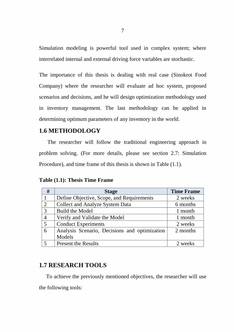
1.6 METHODOLOGY

The researcher will follow the traditional engineering approach in

problem solving. (For more details, please see section 2.7: Simulation

Procedure), and time frame of this thesis is shown in Table (1.1).

Table (1.1): Thesis Time Frame

# Stage Time Frame

1 Define Objective, Scope, and Requirements 2 weeks

2 Collect and Analyze System Data 6 months

3 Build the Model 1 month

4 Verify and Validate the Model 1 month

5 Conduct Experiments 2 weeks

6 Analysis Scenario, Decisions and optimization

Models

2 months

5 Present the Results 2 weeks

1.7 RESEARCH TOOLS

To achieve the previously mentioned objectives, the researcher will use

the following tools:

8

1. Define objectives, scope and requirements: by conducting interviews

with Sinokrot Food Company, represented by GM, production

manager, and sales manager.

2. Data collection: by conducting interviews with GM, production

manager, sales manager, maintenance technician, quality assurance

manager, laboratory technicians, production supervisors, and

inventory manager, by using historical data when is available, and by

watching and monitoring the processes in the company.

3. Data analysis: by using Stat-Fit software which provides good

statistical analysis and statistical experiments design besides to MS.

Excel sheets.

4. Building model: there are many simulation software packages can

be used to build the desired simulation model, such as ARENA,

SIMULAT8, GOLDSIM, ProModel and others. The researcher uses

ARENA software (student version) because it is a simulation

environment consisting of module templates and augmented by a

visual front end. ARENA is suitable to deal with heretical systems

such as main models and sub-models and so on.

1.8 ORGANIZATION OF THE THISES

The thesis begins with introduction chapter to provide the reader with

what the thesis is about in general, how the researcher will deal with thesis

problem, introductory of simulation and tools.

9

The second chapter “SIMULATION” is to give well-defined

simulation, types of simulation, related topics such as analytical modeling

versus simulation modeling, simulation role, simulation advantages and

disadvantages and simulation methodology.

The researcher goes over to mention previous contributions in 3 main

fields; namely supply chain management, production management, and risk

management. Then, the researcher will answer the question of relationship

between this thesis and previous contributions.

To achieve cited objectives, chapter 4 case study (Sinokrot Food

Company) is presented. The researcher described Sinokrot system. Then,

simulation models were built according to simulation methodology. After

that scenarios and decisions were analyzed. Optimization simulation

models were also presented. Finally, the researcher ends the thesis with

thesis conclusions, recommendations and future work.

Detailed Sinokrot system, collected data, analyzed data results, and

details of the simulation models are presented in the appendices.

10

CHAPTER 2

SIMULATION

2.1 SYSTEM, MODEL, AND SIMULATION

Simulation is powerful tool to model studied system. Real dynamic of

systems includes manufacturing, supply chain, information system,

management systems and so on. Model is representative of the real system,

while the simulation is mimic modeling of the system. All of these

terminologies will be explained in the following sections.

2.1.1 SYSTEM

Blanchard defines the system as a collection of elements that function

together to achieve a desired goal. [Blanchard, 1991] The systems have

three types of variables according to C. Harrell et al. [Harrellet al., 2004] as

following:

1. Decision variables (input or independent variables) which affect the

behavior of the system.

2. Response variables (performance or output variables) which measure

the performance of the system in response to particular decision.

3. State variables which indicate the status of the system at any specific

point in time such as the current number of entities waiting to be

processed or the current status (busy, idle, or down such as

unscheduled maintenance) of a particular resource.

11

2.1.2 MODEL

White and Ingalls define the model as simplified abstractions, which

embrace only the scope and level of detail needed to satisfy specific study

objectives. Models are employed when investigation of the actual system is

impractical or prohibitive. This might be because direct investigation is

expensive, slow, disruptive, unsafe, or even illegal. Indeed, models can be

used to study systems that exist only in concept. [White, and Ingalls, 2009]

El- Haik and Al-Aomar classify models as following [El- Haik and Al-

Aomar, 2006]:

Physical Models are tangible prototypes of actual products or

processes.

Graphical Models are abstractions of actual products or processes

using graphical tools.

Mathematical models(Mathematical modeling) is the process of

representing system behavior with formulas or mathematical

equations

Computer Models are numerical, graphical, and logical

representation of a system (a product or a process) that utilizes the

capability of a computer in fast computations, large capacity,

consistency, animation, and accuracy.

12

2.1.3 SIMULATION

In English, the simulation can be defined as a way” to reproduce the

conditions of a situation, as means of a model, for study or testing or

training etc.” [Oxford American Dictionary, 1980] Harrell et al. defined

simulation as the “imitation of a dynamic system using a computer model

in order to evaluate and improve system performance.” [Harrell et al,

2004], Kelton et al. refer it to a board collection of methods and

applications to mimic the behavior of real systems” [Kelton et al., 2001],

on the other hand, Bangsow defined simulation as the reproduction of a real

system with its dynamic processes in a model. The aim is to reach

transferable findings for the reality. In a wider sense, simulation means

preparing, implementing, and evaluating specific experiments with a

simulation model. [Bangsow, 2010]

In this thesis, simulation can be defined as a mimic methodology uses

computer technology or software to model a system which deals with

complexity of stochastic input data and interrelated (interdependent)

internal and external variables besides to multi criteria making decision in

order to study the system behavior based on determined parameters, test

desired situations or scenarios, detect system problems, develop the system,

optimize system efficiency and effectiveness.

The system from simulation perspective consists of entities,

activities, resources, and controls. As shown in Figure (2.1) these elements

13

define the “who, what, where, when, and how of entity processing. Entities

such as customers are items processed through performing activities in the

system by means called resources which perform the activities, while the

control is how, when, and where activities are performed such as routing

sequences, work schedules, instruction sheets, and task prioritization.

Figure (2.1): Elements of a system from simulation prospective, [Harrell et al, 2004]

2.2 TYPES OF SIMULATION

White and Ingalls categorize simulation types as the following [White, and

Ingalls, 2009]:

Static versus Dynamic

Static simulation is one that is not based on time, where the dynamic

simulation includes the passage of time. It looks at state changes as they

occur over time. According to this description, simulation system of the

case study in this thesis is considered as dynamic simulation system.

14

Stochastic Versus Deterministic

Simulations -in which one or more variables are random- are referred to

as stochastic or probabilistic simulations. A stochastic simulation produces

output itself random and therefore gives only one data point of how the

system might behave, while simulations which have no input components

that are random are said to be deterministic. Based on this description,

simulation system in this thesis is considered as stochastic simulation

system.

Discrete Event Versus Continuous Simulation

A discrete event simulation is one in which state changes occur at

discrete points in time as triggered by events. In continuous simulation,

state variables changes continuously with respect to time and therefore

referred to as continuous (change state variables such as level of oil in an

oil tanker that is being either loaded or unloaded). The simulation system of

the case study is considered discrete event simulation.

So the case study (Sinokrot Food Company) is dynamic, stochastic, and

discrete event Simulation.

Analytical Modeling Versus Simulation Modeling

Altiok and Melamed differentiated between analytical and simulation

solutions or performance measures, where the analytical models calls for

the solution of mathematical problem, the derivation of mathematical

15

formulas, or more generally, algorithmic procedures. The solution is then

used to obtain performance measures of interest.

On the other hand, “a simulation model calls for running (executing) a

simulation program to produce sample histories. A set of statistics

computed from these histories is then used to form performance measures

of interest.”[Altiok, and Melamed, 2007]

In this thesis, it is focused on simulation system because of system

complexity referred to stochastic variability and interrelated

(interdependencies) of the system variables, where analytical modeling

cannot deal with what appears in the case study.

2.3 ROLE OF SIMULATION

El- Haik and Al-Aomar clarify the role of simulation by first justifying

the use of simulation both technically and economically and then

presenting the spectrum of simulation applications to various industries in

the manufacturing and service sectors. The role can be summarized in the

following points [El- Haik and Al-Aomar, 2006]:

A. Simulation Justification

1. Technical Justifications

Simulation capabilities are unique and powerful in system

representation, performance estimation, and improvement.

16

Simulation is often utilized when the behavior of a system is

complex, stochastic (rather than deterministic), and dynamic (rather than

static).

Analytical methods, such as queuing systems, inventory models, and

Markovian models -which are commonly used to analyze production

systems-often, fail to provide statistics on system performance when real-

world conditions intensify to overwhelm and exceed the system

approximating assumptions.

Decision support encountering critical stages of design so that

designers reveal insurmountable problems that could result in project

cancellation, and save cost, effort, and time.

2. Economical Justifications

Although simulation studies might be costly and time consuming in

some cases, the benefits and savings obtained from such studies often

recover the simulation cost and avoid much further costs.

Simulation can reduce cost, risk, and improve analysts’

understanding of the system under study.

B. Simulation Applications

Wide spectrum of simulation applications to all aspects of science

and technology

Utilizing simulation in practical situations and designing queuing

systems, communication networks, economic forecasting, and strategies

and tactics.

17

2.4 SIMULATION ADVANTAGES

Zandian remarks simulation advantages in the following points [Zandian,

2004]:

Increase in Global Competition

In the last 20 years, almost all businesses have provided products and

services globally, so that pressures exerted on them to increase their

competitiveness by using simulation tools for testing implementations of

continuous productivity improvement, process reengineering, and the best

alternative system design.

Cost Reduction Efforts

Simulation modeling becomes an essential tool to increase the robustness

of the system relative to internal and external disturbances in design of lean

or agile systems to increase production rates and flexibility while reducing

the investments in inventories, equipment, and labor.

Improved Making Decision

Simulation modeling has been proved as an effective tool in training

managers because they can understand the effects of their decisions on the

important performance metrics of the system. And also “Simulation avoids

the expensive, time-consuming, and disruptive nature of traditional trial-

and-error techniques.”[Harrell et al, 2004]

18

Effective Problem Diagnosis

Simulation models can solve a problem at different levels of details and

complexity with the credibility management requires for effective use in

real-life situations rather than other analytical tools such as mathematical

techniques, artificial intelligence, statistical techniques, and root cause

analysis techniques, which either require too many simplistic assumptions

to solve the problem or are too complex to be explained credibly to

management.

Prediction and Explanation Capabilities

Simulation modeling provides both prediction and explanation of a

system’s performance under different conditions. In addition to predicting

what the system’s performance will be for a set of conditions, the user can

also comprehend the reasons why the system produces those results and

behaves in a certain way.

Risk Analysis

Flangagan and Norman mention probability analysis as a powerful tool in

investigating problems which do not have a single value solution.

Simulation is the most easily used form of probability analysis. It makes

the assumption that parameters subject to risk and uncertainty can be

described by probability distributions. [Flangagan and Norman, 1999]

19

C. Chung added the following points [C. Chung et al, 2004]:

Experimentation in Compressed Time

Because the model is simulated on a computer, experimental simulation

runs may be made in compressed time and so that multiple replications of

each simulation run can easily be run to increase the statistical reliability of

the analysis. Thus, systems that were previously impossible to be analyzed

robustly can now be studied.

Reduced Analytic Requirements

Before the existence of computer simulation, only simple systems that

involved probabilistic elements could be analyzed by the average

practitioner. More complex systems were strictly the domain of the

mathematician or operations research analyst. In addition, systems could be

analyzed only with a static approach at a given point in time. In contrast,

the advent of simulation methodologies has allowed practitioners to study

systems dynamically in real time during simulation runs.

Easily Demonstrated Models

The use of animation during a presentation can help establish model

credibility. Animation can also be used to describe the operation and

interaction of the system processes simultaneously. This includes

dynamically demonstrating how the system model handles different

situations.

20

2.5 DISADVATAGES OF SIMULATION

According to [Chung et al., 2004] simulation modeling has specific

disadvantages, given as follows:

Simulation Cannot Give Accurate Results When the Input Data

Are Inaccurate (garbage-in-garbage-out (GIGO))

The results obtained from simulation models are as good as the model

Data inputs, assumptions, and logical design. Data collection is considered

the most difficult part of the simulation process.

Simulation Cannot Provide Easy Answers to Complex Problems

If the system analysis has many components and interactions, the best

alternative operating or resource policy is likely to consider each element

of the system. It is possible to make simplifying assumptions for the

purpose of developing a reasonable model in a reasonable amount of time.

However, if critical elements of the system are ignored, then any operating

or resource policy is likely to be less effective.

Simulation Alone Cannot Solve Problems

Simulation provides the management with potential solutions to solve the

problem. Potential solutions are developed but are never or only poorly

implemented because of organizational inertia or political considerations.

21

2.6 WHEN SIMULATION IS APPROPRIATE

According to Harrel et al. [Harrell et al, 2004], Simulation is appropriate

if the following criteria hold true:

An operational (logical or quantitative) decision is being made.

The process being analyzed is well defined and repetitive.

Activities and events are interdependent and variable.

The cost impact of decision is greater than the cost of doing the

simulation.

The cost of experiment in the actual system is greater than the cost of

simulating it.

In this thesis, simulation modeling is an appropriate analysis tool for

the case study (Sinokrot Food Company) because of well-defined and

repetitive process such as production, interdependency variables such as

produced quantities, break down times and frequency, availability of raw

materials, readiness of production lines, and also logic operational is used

in scheduling production. Besides the cost of simulation in negligible when

it is compared to actual system costs.

2.7 SIMULATION METHODOLOGY

Simulation analyst follows a generic and systematic approach for

applying a simulation study effectively. This approach is atypical

engineering methodology for system design, problem solving, or system

22

improvement. It consists of common stages for performing the simulation

study as shown in the figure (2.2).

Harrell et al mention the following steps [Harrell et al., 2004]:

Figure (2.2): Iterative nature of simulation,[Harrell et al., 2004]

2.7.1 STEP 1: DEFINING OBJECTIVE, SCOPE, AND REQUIREMENTS

Simulation objectives can be grouped into the following general categories:

Performance analysis – What is the all-around performance of the

system in terms of resource utilization, flow time, output rate, etc.

Capacity or constraint analysis – What is the production capacity of

the system and where are the bottlenecks?

23

Configuration comparison –How well does one system configuration

meet performance objectives compared to another?

Optimization –When are the settings for particular decision variables

best achieve desired performance goals?

Sensitivity analysis – Which decision variables are the most

influential on performance measures, and how influential are they?

Visualization –How can system dynamics be most effectively

visualized?

An important part of the scope is a specification of the models that will

be built (as-is model), when evaluating improvements to an existing

system; it is often desirable to model the current system first. This is called

an “as-is” model. Results from the as-is model are statistically compared

with output of the real-world system to validate the simulation model. This

as-is model can then be used as a benchmark or baseline to compare the

results of “to-be” models. With the scope of work defined, resources,

budget and time requirements can be determined for the project.

2.7.2 STEP 2: COLLECTING AND ANALYZING SYSTEM DATA

The steps of gathering data should follow this sequence:

Determine data requirements and identify data sources.

Collect the data (such as entity flow).

Make assumption where necessary.

Analyze the data (such as distribution fitting).

24

Document and approve the data.

2.7.3 STEP 3: BUILDING THE MODEL

The conceptual model is the result of the data-gathering effort and is

a formulation in one’s mind (supplemented with notes and diagrams) of

how a particular system operates. Building a simulation model requires that

this conceptual model to be converted to a simulation model. The

simulation model consists of structural elements (entities, location,

resources) and operational elements (routings, operations, entity arrivals,

entity and resource movement)

2.7.4 STEP 4: VERIFYING AND VALIDATING THE MODEL

“Verification is the process of determining whether the simulation model

correctly reflects the conceptual model.” [Harrell, 2004] or verification is

“ensuring that the simulation model has all the necessary components and

that the model actually runs. In reality, it is interested in getting the model

not just to run but to run the way we want it to. In other words, it is

interested in ensuring that the model operates as intended. Another way to

look at the verification processes is to consider it as: Building the model

correctly.”[Chung et al., 2004]

"Validation is focused on the correspondence between model and reality:

are the simulation results consistent with the system being analyzed? Did

25

we build the right model? Based on the results obtained during this phase,

the model and its implementation might need refinement.”[Wainer, 2009]

Harrell et al. argue the use of combination of techniques when a validating

a model such as watching the animation, comparing with actual system,

comparing with other model, conducting degeneracy and extreme condition

tests, checking for face validity, testing against historical data, performing

sensitivity analysis techniques, running traces, and conducting tests.

[Harrell et al., 2004]

2.7.5 STEP 5: CONDUCTING SIMULATION EXPERIMENTS

When executing the simulation model by following the goals stated

in the conceptual model, it is needed to evaluate the outputs of the

simulator, and using statistical correlation to determine a precision level for

the performance metrics. “This phase starts with the design of the

experiments, using different techniques. Some of these techniques include

sensitivity analysis, optimization, variance reduction (to optimize the

results from a statistical point of view), and ranking and selection

(comparison with alternative systems).” [Wainer, 2009]

2.7.6 STEP 6: PRESENT THE RESULTS

Simulation outputs are analyzed in order to understand the system

behavior. These outputs are used to obtain responses about the behavior of

the original system. “At this stage, visualization tools can be used to help

26

with the process. The goal of visualization is to provide a deeper

understanding of the real systems being investigated and to help in

exploring the large set of numerical data produced by the simulation.”

[Wainer, 2009]

27

CHAPTER 3

LITER ATURE REVIEW

Simulation modeling is used in many fields, such as supply chain

management, transportation, logistics, manufacturing, reengineering

processes, maintenance, optimization, risk management, layout design,

project management, and etc.

In this chapter, the literature reviews of supply chain management,

manufacturing management, and risk management is presented.

3.1 SUPPLY CAHIN

The objective of supply chain management is to meet customer demand

for guaranteed delivery of high quality and low cost with minimal lead

time.

Some of inefficiencies in the business can be found from suppliers or in the

business processes themselves. So simulation according to Chang et al. can

helps companies to understand the overall supply chain processes and

characteristics to be able to capture system dynamics, to model unexpected

events in certain areas and understand the impact of these events on the

supply chain as well as being able to dramatically minimize the risk of

change in planning process. [Chang et al., 2002]

And also Chang et al, in order to analyze the supply chain, simulator

should use operating performance prior to the implementation of the

28

system, perform what-if analysis to lead better planning decisions, and

compare of various operational alternatives without interrupting the real

system.[Chang et al., 2002]

Hellström et al. used simulation in analyzing a case study to model

both operational (material handling) and tactical (order process, inventory

management) supply chain scenarios. The response from the model was

that the material handling procedures became faster and more accurate,

resulting in less utilization of resources. While in tactical planning,

simulation had the ability to tell how the retail supply chain performed and

behaved when different ordering rules were used. [Hellström et al., 2002]

X. Qi developed an integrated making decision model for a supply

chain system where a manufacturer faces a price-sensitive demand and

multiple capacitated suppliers. “The goal is to maximize total profit by

determining an optimal selling price and at the same time acquiring enough

supplying capacity.”[Qi, 2007]

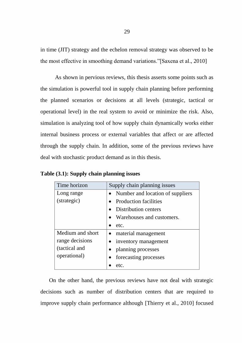
Thierry et al. focus on the role of modeling and simulation in

studying various issues in supply chain management based on time horizon

decisions [Thierry et al., 2010] as shown in Table (2.1).

Saxena et al. presented a simulation model to analyze the effect of

different ordering policies and different set of parameters for different

nodes of supply chain on a cost and time performance. It was founded just-

29

in time (JIT) strategy and the echelon removal strategy was observed to be

the most effective in smoothing demand variations.”[Saxena et al., 2010]

As shown in pervious reviews, this thesis asserts some points such as

the simulation is powerful tool in supply chain planning before performing

the planned scenarios or decisions at all levels (strategic, tactical or

operational level) in the real system to avoid or minimize the risk. Also,

simulation is analyzing tool of how supply chain dynamically works either

internal business process or external variables that affect or are affected

through the supply chain. In addition, some of the previous reviews have

deal with stochastic product demand as in this thesis.

Table (3.1): Supply chain planning issues

Time horizon Supply chain planning issues

Long range

(strategic)

Number and location of suppliers

Production facilities

Distribution centers

Warehouses and customers.

etc.

Medium and short

range decisions

(tactical and

operational)

material management

inventory management

planning processes

forecasting processes

etc.

On the other hand, the previous reviews have not deal with strategic

decisions such as number of distribution centers that are required to

improve supply chain performance although [Thierry et al., 2010] focused

30

on the role of simulation modeling based on time horizon, and [Saxena et

al., 2010] deled with some strategies (JIT).Also, they deled with one

product, while this thesis deals with multi-products sharing with

interrelated raw materials which are determined by bill of materials (BOM)

for each product.

3.2 INVENTORY MANAGMNET

Inventory management is an important tool to mitigate the risks arising

due to Supply failures. Cannella et al. conclude that an increment of

production capacity does not necessarily improve customer service without

demand amplification. Risk in this case is due to satisfying at a higher cost

an over-estimated market demand. [Cannella et al., 2008]

Samvedi et al. developed a simulation model to study which inventory

method will be the best for such situations and the impact of periodic

inventory parameters values on supply disruption situations. Moreover, the

research led to that the cost of the players in the chain increases with

increasing maximum inventory level and decreases with increasing review

period.[Samvedi et al., 2011]

Alizadeh et al. developed an inventory simulation model to reduce total

inventory cost when demand and lead time are stochastic variables. In

addition, they used optimization to determine the optimal or near optimal

lead time to minimize the inventory total cost. [Alizadeh et al., 2011]

31

Akcay et al. studied estimation of inventory targets when demand

process is auto-correlated and only a limited amount of historical data is

available. A developed simulation model was used to expect the cost due to

demand parameter uncertainty, and to obtain the value of the bias

parameter to reduce the impact of parameter uncertainty in inventory-target

estimation. [Akcay et al., 2012]

As shown in pervious reviews, simulation models were developed to

study impact of increment of production capacity, periodic inventory

parameters, inventory targets, or to minimize total inventory cost when

demand and lead time are stochastic. Indeed, simulation can be used to

model real inventory system where demand and lead time are stochastic,

need to determine optimal inventory target level, optimal reorder point and

optimal order quantity for fixed-ordered-quantity system, optimal

reviewing time for fixed-time-reviewing system, optimal inventory

capacity, and so on.

3.3 MANUFACTURING MANAGMENT

PRODCUTIION PLANNING AND SCHEDULING

Vasudevan et al. presented the integration use of process simulation,

production scheduling, and material handling. Several suggested

improvements were simulated and analyzed. These improvements increase

productivity by 47% and annual revenue $1,800,000. [Vasudevan et al.,

2008].

32

Wu et al. introduced an integrated dynamic simulation model for

multi-workstation production systems. The model is used to analyze the

fundamental properties and dynamic behavior of multi-workstation

production systems. As a result; “the low variation of the lead time at each

workstation indicated simulation was able to predict lead times based on

real production data. The predicted lead time can be used to plan

production in common static capacity planning systems used in industry,

such as MRP.” [Wu et al., 2008]

Sun et al. developed a multi-item MRP (Material Requirements

Planning) simulation model to study the effects of factors such as forecast

errors, process variability, and levels of updating frequency on the

performance of MRP system in terms of average inventory and fill rate

under different operating conditions.[Sun et al., 2009]

Hübl et al. introduced a simulation model for analyzing production

systems. The model included stochastic behavior for customer

performance, processing times, set up times and purchasing lead time.

The model combines three hierarchical levels; the highest level: MPS

(Master Production Schedule) which calculates the aggregated production

program. The midterm level: two PPC (Production Planning and Control)

methods MRPII and Conwip (Constant Work in process).and lowest level,

different dispatching rules. The interactions between the levels were tested

and manufacturing system was analyzed [Hübl et al, 2011]

33

In my point view planning and scheduling simulation models -as

shown in previous literature reviews- are useful when dealing with

planning input variables such as stochastic customer behavior, stochastic

market demand, net requirement quantities, delivery time, resources, etc. in

addition, planning and scheduling scenarios are simulated to find the best

scenario. These models were built to study of real systems and their

performance measures such as resources utilization, fill rate, lead time, etc.

on the other hand, planning and scheduling models are effected when

multiple products share raw materials determined by bill of material for

each product. These interrelated variables will be undertaken in this work.

BOTTELNECKS DETECTION AND ELIMINATION

Sengupta et al. present a method to identify and rank the bottlenecks

in a manufacturing system by using simulation techniques. The proposed

method was based on analyzing inter-departure time from different

machines, the duration of machine being active without interruption, and

utilization of machines. It was founded that bottle necks were detected

where the machine with the highest utilization, and the machine with the

longest average up-stream queue length. [S. Sengupta et al, 2008].

Moreover, Pawlewski et al. presented simulation model to describe

the elements of the production system in the relationships between them

and to analyze when resources were required and when were available in

the same time frame. [Pawlewski et al., 2010]

34

This thesis is based on the previous reviews. So that bottlenecks can

be detected by measure performance variables such as duration production

line being active (or more detailed machines in the production line) without

interruption, utilization either daily production utilization (real production

time to available production time) or annual utilization (number of

production periods to available annual production periods).

MAINTENACE MANAGMENT

Ali et al. presented simulation optimization model to minimize

maintenance investment and system downtimes. The model was based on

optimization selection for maintenance polices optimization system design,

and optimization maintenance scheduling schemes in order to evaluate

these variables on the overall system performance.[Ali et al., 2008]

Altuger et al. developed maintenance simulation to analyze

production line performance and equipment utilization. The model assessed

different preventive maintenance scheduling techniques to select the best.

Maintenance scheduling techniques included: Global Maintenance Order

(GMO), Reliability-Based Maintenance Order (RMO) and Value-Based

Maintenance Order (VMO). [Altuger et al., 2009]

Breakdowns in general can be defined as causes make the production line

or machine stop. Therefore breakdown can include scheduled maintenance,

unscheduled maintenance, parts shortage, and reproduction.

35

SETUP TIME REDUCTION

Kämpf et al. explores the optimal sequencing and lot size problem

for a stochastic production and inventory system with multiple items. The

system consists of a single-stage-multiple-product type manufacturing unit

that has to meet a random demand for N items. Simulation model was

developed to find optimal sequencing and lot size parameter values that

maximize expected profit per time unit. [Kämpf et al., 2006]

Grewal et al. investigate the benefits of setup time reduction and lot

size optimization as well as reorder point optimization as decision

variables. Discreet event simulation model was developed to study the

effect of cited decision variables on performance variables such as total

inventory and customer service levels. It was found that setup time

reduction alone reduces the total system inventory required to meet a

specific customer fill rate, and the optimal lot sizes decrease significantly

with reduced setups. In addition, lot sizes are found to be slightly smaller at

increased service level targets. [Grewal et al., 2009]

Setup time reduction affects the performance measures, total inventory, and

customer fill rate positively. Setup times can be reduced also by adopting

some production management polices as will be shown in the thesis.

36

LEAN MUNIFACTURING

“Lean is the set of ‘tools’ that assist in the identification and steady

elimination of waste (muda), the improvement of quality, and production

time and cost reduction.”[Wilson, 2010] The wastes include over

production, transportation, unnecessary inventory, inappropriate process,

activity resulting from rejected product, unnecessary motion, knowledge

disconnections, and unused creativity.

Heilala et al. proposed an integrated simulation tool to maximize

production efficiency and balance environmental constraints already in the

system design phase. They used simulation to identify production waste

(e.g. waiting, work in process, inventories, and transportations), Value

Stream Mapping (VSM) and other process modeling methods. Then they

developed scenarios to eliminate these wastes. [Heilala et al., 2008]

Brown et al. presented a simulation model to study “the ability to

identify cost reduction opportunities through improving operational

efficiencies provides companies with the ability to reduce costs while

maintaining service levels”.[Brown et al., 2009]

Gregg et al. presented an approach for modeling manufacturing process

flows. Simulation incorporates a work flow schedule to model cycle time

and resource usage, accounting for task sequencing, task duration

variability, resource requirements (labor, tooling, position, etc.), maximum

capacity, and contention. “The approach has been used successfully within

37

Boeing to support analysis and cycle time reduction of aircraft and

spacecraft production flows and resource requirements analysis including

labor and equipment.”[Gregg et al., 2011]

Mahfouz et al. developed simulation based optimization model to

evaluate the lean implementation in SME (Small to Medium Enterprise)

packaging manufacturer. Four lean factors have been defined; demand

management, preventive maintenance, labor capacity, and production flow,

and examined against three response functions, cycle time, WIP (Work in

Process) and staff utilization.

“The model has contributed significantly to develop a better understanding

of the system dynamics (i.e. impact on overall performance) through the

factor analysis phase.”[Mahfouz et al., 2011]

In my point view; simulation means simulating the real system,

studying system behavior, detecting manufacturing wastes, developing

scenarios to eliminate the wastes, and analyzing system performance.

3.4 RISK MANAGEMENT

“Risk can be defined as the probability of occurrence of an event that

would have a negative effect on a goal.” [Vose, 2000]

Lesnevski et al. presented a procedure for generating a fixed-width

confidence interval for a coherent risk measure. Coherent risk measures

based on generalized scenarios were viewed as estimating the maximum

38

expected value from among a collection of simulated “systems”. The

procedure improved upon previous methods by being reliably efficient for

simulation of generalized scenarios and portfolios with heterogeneous

characteristics. [Lesnevski et al., 2006]

Chen et al. presented simulation model to evaluate product prices and

to estimate the risk measures of portfolio. [Chen et al., 2007]

Better et al. explored applications of simulation optimization

involving risk and uncertainty due to simulation optimization capabilities,

quality of solutions, interpretability, and practicality. They demonstrated

advantages of using a Simulation Optimization approach to tackle risky

decisions by show casing the methodology on two popular applications

from the areas of finance and business process design. [Better et al., 2008]

Hennet et al. analyze the risks incurred by supply chains-both

externally and internally- which present several alternatives to evaluate the

risks of disruption of a supply chain and bankruptcy of one or several of its

member enterprises that discuss the integration of risk management within

classical supply chain management approaches. [Hennet et al., 2009]

In point view; there are some risk issues as shown in the previous

reviews. Simulation can measure risk by analyzing the model behavior,

suggesting scenario to reduce or eliminate the risk, and evaluating the total

performance. These theses will highlight internal and external risks in

manufacturing, Inventory, and supply chain systems.

39

CHAPTER 4

CASE STUDY

4.1. SINOKROT FOOD COMPANY

Sinokrot Food Company is based in Baytonia industrial zone in Ramallah

and Al-Bireh governance –West Bank. It produces more than 60 products

through 8 modern production lines according to international quality and

health standards. Some of these products are Ali Baba, Ali Baba- Gifts,

Jericho Wafer, Sinokrot Wafer, Sababa Nougat, Marsh, Zaki, Toffee Nut,

Rollo, Rolls Royce, Noody Loose, Noody 48 pieces, Marie Biscuit, Family

Cookies 300 gm, Family Cookies 600 gm, Jammy, Noody tubes,. It has a

local market share of about 30% and exports its products to Jordan, Saudi

Arabia, USA and England. It is the first Palestinian company that obtained

the ISO 2000 certificate in the year 1996. It is also the first Palestinian and

Arab food company that was able to develop and produce fortified food

products so as to participate in solving the malnutrition dilemma among

children. It distributes its products to more than 4000 outlets in the local

market. Among the notable business partners are the World Food Program

(WFP), American Near East Refugee Aid (ANERA) and the Islamic Bank

for Development.

40

4.2 SINOKROT SYSTEM

4.2.1 PRODUCTION

Production system in SFCo includes 8 production lines to produce 60final

products. Production rates, daily produced quantity, production lines

breakdown times and frequencies are stochastic variables. The following

sections describe in more details of production system.

PRODUCTS

Sinokrot Food Company (SFCo.) produces more than 60 products, 98% of

them are semi-daily produced, while others are produced rarely or when are

demanded. Semi-daily produced products are 20 products, and they are

denoted in simulation system by PR; as abbreviation of products.

PRODUCTS GROUPING

SFCo owns 8 production lines. Each production line produces alike

products called “products groups”, i.e. “production line 1” produces

“products group 1” ,”production line 2” produces “products group 2” and

so on, as an exception of this rule, “ production line 1” produces “products

group 2” if the line is not busy.

“products group 1” includes “product 1” and “product 2”, while “products

group 2” includes “product 3”, product 4”, product 5”, and “product 5”.

Table (A.1) in Appendix A shows these products groups. These products

groups are obtained by interviewing the production manager.

41

PRODCUTIO PERIODS

The production system of SFCo includes 2 production periods; the first

begins in 7:30 to 16:00 (production time is 8.5 hours), while the second

begins 16:00 to 23:30 (production time is 7.5 hours) as obtained from daily

production reports.

PRODUCTION RATES

Production rate can be expressed by produced quantities per production

period. In our case, production line rate of each product varies refers to

considered reasons related to human power, quality of raw material,

reproduction, breakdowns and unscheduled maintenance. In addition, the

production rate is a stochastic variable by which the value changes

according to product and production period.

In our case, production rate is defined as in term of actual time consumed

(second) to produce 1unit (1carton case, or 1 kg for “product 11”). Data of

production rate is obtained from daily production reports for 12 months,

calculating net production time (after removing breakdowns time), and

calculating production rate by dividing net production time by produced

quantity as shown in EQ.1. The calculated production rates were compared

with production rates obtained by sit watching and monitoring (samples).

The result of comparing assured that homogeneity of both sources of data,

besides to discussing them with production manager.

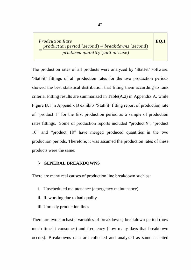
42

EQ.1

The production rates of all products were analyzed by ‘StatFit’ software.

‘StatFit’ fittings of all production rates for the two production periods

showed the best statistical distribution that fitting them according to rank

criteria. Fitting results are summarized in Table(A.2) in Appendix A. while

Figure B.1 in Appendix B exhibits ‘StatFit’ fitting report of production rate

of “product 1” for the first production period as a sample of production

rates fittings. Some of production reports included “product 9”, ‘product

10” and “product 18” have merged produced quantities in the two

production periods. Therefore, it was assumed the production rates of these

products were the same.

GENERAL BREAKDOWNS

There are many real causes of production line breakdown such as:

i. Unscheduled maintenance (emergency maintenance)

ii. Reworking due to bad quality

iii. Unready production lines

There are two stochastic variables of breakdowns; breakdown period (how

much time it consumes) and frequency (how many days that breakdown

occurs). Breakdowns data are collected and analyzed as same as cited

43

production rates, and summarized for all production lines in Table (A.3) in

Appendix A.

PRODUCTION MANAGEMENT

Production management is based on:

i. Checking maximum inventory shortage of a product among products

in the same product group. Product inventory shortage is

EQ.2

ii. Checking availability of raw material used to produce the expected

quantities.

iii. To utilize setup time there was no change product through

production periods. The change occurs only at beginning of them.

4.2.2 RAW MATERIALS INVENTORY MANAGEMENT

SFCo consumes many raw materials to produce more than 60 products.

SFCo purchases these materials from local suppliers and or international

suppliers. Also, it assures the quality when receipts them. Number of raw

44

materials is more than 100 but they can be grouped in 11 groups, namely

RM1, RM2… and RM11.

RAW MATERIALS INVENTORY MANAGEMENT

Raw material inventory management is periodic order; some of raw

materials are ordered every 26 working days (month), and some of them

are ordered every 20 working days. There was no accurate historical of

ordered quantities because some of raw materials were sold to other

manufacturers. Therefore, the ordered quantities and reorder points were

assumed to be correct according to production manager experience. Table

(A.4) in Appendix A exhibits the raw material order frequency, ordered

quantities and reorder point.

RAW MATERIALS RISK

Some factors affect the raw material ordered quantities and reviewing times

such as international or local suppliers, purchasing lead time, fluctuate

draw material prices, and Israeli occupation polices.

BILL OF MATERIALS

Table (A.5) in Appendix A exhibits product structure of components (raw

materials) according to laboratory supervisor. Bill of material is expressed

by weight to produce one case of product.

45

4.2.3 DISTRIBUTION CENTERS AND PRODUCT DEMAND

Distribution centers are very important components of the supply chain.

Sinokrot Food Company (SFCo) provides Palestinian market with its

products through 5 distribution centers distributed in West Bank.

Distribution centers provide the company with required products

(customers’ orders), and receipt the finished products to deliver them to the

customers.

The distribution centers are denoted in simulation system by DC; as

abbreviation of Distribution Center.

TOTAL DAILY PRODUCT DEMAND

Total daily product demand for any product is sum of distribution centers

demands as shown in EQ.3. Daily demands of any product were obtained

from historical reports (for 12 months). all of these daily demands were

grouped for each month and analyzed by using ‘StatFit’ software to fit

them with best statistical distribution as shown in Table (A.6) in Appendix

A. Figure B.1 in Appendix B exhibits ‘StatFit’ fitting report of total daily

“product 6” demand as an example.

EQ.3

46

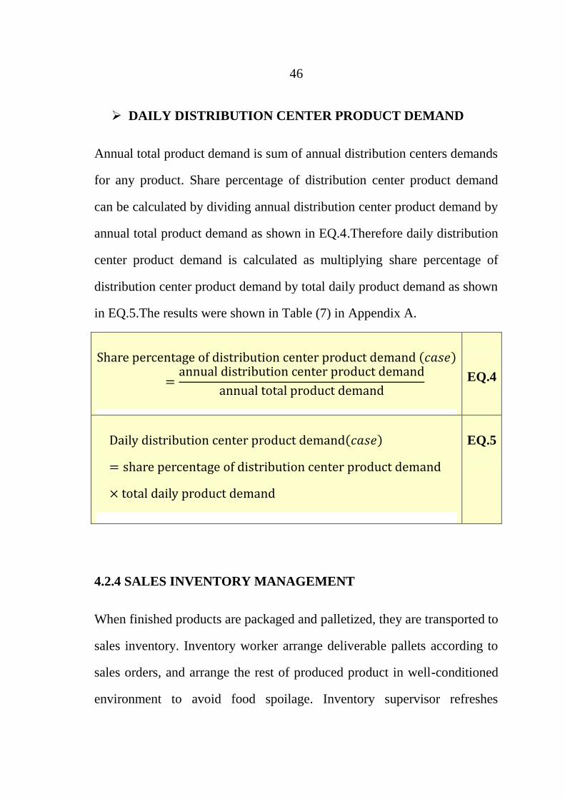
DAILY DISTRIBUTION CENTER PRODUCT DEMAND

Annual total product demand is sum of annual distribution centers demands

for any product. Share percentage of distribution center product demand

can be calculated by dividing annual distribution center product demand by

annual total product demand as shown in EQ.4.Therefore daily distribution

center product demand is calculated as multiplying share percentage of

distribution center product demand by total daily product demand as shown

in EQ.5.The results were shown in Table (7) in Appendix A.

EQ.4

EQ.5

4.2.4 SALES INVENTORY MANAGEMENT

When finished products are packaged and palletized, they are transported to

sales inventory. Inventory worker arrange deliverable pallets according to

sales orders, and arrange the rest of produced product in well-conditioned

environment to avoid food spoilage. Inventory supervisor refreshes

47

inventory level when he receipts or back finished product up to

transporters.

SALES INVENTORY CAPACITY

Sales inventory consists of 3 vertical layers to utilize the sales inventory

space; sales inventory is capable to store 200 pallets of products. Sales

department determined target level by their experience for each product so

that to avoid product shortage to fulfill distribution center demand. Table

(A.8) in appendix A exhibits product target level.

SALES INVENTORY MANAGEMENT

The main principle in food inventory is FIFO (first in, first out) because it

keeps material or product in good quality and safety.

Inventory monitoring principle is based on product inventory level, safety

stock level, the product demand, and booked order demand. To determine

which product is most required among the product group, it have to be the

higher production priority which can be defined as the difference between

product sales inventory target in addition to booked sales and product sales

inventory level.

Sales inventory input is presented by produced quantity of a product, while

sales inventory output is presented by product sold quantity. Following

equation EQ.6 presents product sales inventory level in a certain time

period (i).

48

EQ.6

4.2.5 SALES, PALLETIZING AND TRANSPORTATION

The last operations that SFCo performs before deliveries the final products

are palletizing the required products and arranging them in such manner

according to transporter capacity i.e. 10-12 pallets.

SALES AND PALLETIZING

To prepare ordered quantity of products, they must be palletized. Ordered

quantities can be rounded to quarter of pallet. Table (A.9) in Appendix A

exhibits number of cases per pallet.

TRANSPORTATION

SFC owns 5 transporters to deliver the products to the 5 distribution

centers; each transporter is capable to deliver 10-12 pallets per charge. The

transportation time depend on the distance between the sales inventory and

distribution center, and Israeli occupation obstacles.

49

TRANSPORTATION RISK

Israeli occupation policies affect transportation time; the policies are

reflective of security and general policy in Israel. So, transportation time is

dependent factor varies from time to time.

4.2.6 GENERAL CONCEPTUAL MODEL

Conceptual model is a represent of the actual system or real life system

under study. The general conceptual model of Sinokrot system is shown in

Figure (4.1).

4.3. PROBLEM DIFINITION AND OBJECTIVES

Analytical making decision process is very hard one when dealing with

stochastic input variables and complex interrelated variables. To overcome

this problem, simulation techniques are used in making decision at all

levels; strategic, operational, and tactical level.

50

DISTRIBUTION

CENTERS

PRODCUT

DEMANDS

SALES

INVENTORY

DELIVERY

MANAGMENT

TRANSPOR-

TATION

DISTRIBUTION

CENTERS

PRODCUT SALES

PRODCUTION

PLANNING AND

SCHEDULING

PRODCUTION

MATERIAL

REQUIRMENT

PLANNING

MATRIAL

INVENTORY

MAIN SINOKROT DELIVERY

Figure (4.1): General Sinokrot conceptual model

Simulation modeling of: supply chain, manufacturing system, and risk

management is a cornerstone of simulation applications for many years.

Recently, there has been an increasing interest in excellence in evaluating

the real system proposed scenarios or decisions and optimization system

parameters.

According to the case study, there are many objectives in simulating the

real life system in order to achieve the organization objectives:

1. Develop real model (ad-hoc model), to evaluate current parameters

and performance indicators of supply chain, manufacturing system,

and risk management.

51

2. Develop simulation models to evaluate decisions or scenarios in

order to achieve organization objectives at all levels; strategic,

operational, and tactical levels.

3. Develop optimization simulation model to design or re-design

inventory management parameters to minimize inventory costs,

minimize stored quantity according to lean manufacturing

philosophy, and maintain stock-out percentage less than a specific

point.

4.4 SIMULATION MODEL AND DESCRIPTION

Before describing the simulation model, some ARENA terms are required

to be understood as well as the abbreviations that used in this thesis

(especially in the following equations) as shown in Table (4.1).

Simulation model is composed of two separated simulation models; the

first is "Main Sinokrot simulation" model, while the second is "Delivery

simulation" model. The output of main Sinokrot simulation model is the

input data of the delivery simulation model by using MS Excel sheet

named “Main Sinokrot simulation” to overcome problems and constraints

of student version of ARENA Software such as limited number of modules

and variables.

Main Sinokrot simulation model is composed of creation entities creation

module in addition to 3 branches or stations named; “product demand and

sales”, “production planning management and production”, “and raw

52

material management”. Creation entities modules create entities and assign

their sequence or future stations or branches that will enter. Number of

daily created entities in simulation model is 131 entities which are named

orders assigned as in Table (4.2).

Table (4.1): Used ARENA terms and abbreviations

Term Meaning Used

Abbreviation

Attribute store information for each entity

common characteristic of all entities

, but with a specific value than differ

from one entity to another

values are tied to a specific entities

[att.]

Expression Predefined or set values such as

constants

[exp.](argument

1, argument 2)

Variables

(global)

Store some real-valued quantity that

can be reassigned during the

simulation run.

They can be vector or matrix as

dimensional tables of individual

values.( one- or two-dimensional

arrays)

(argument

1)[1dVar.] for

one-

dimensional

array

(argument 1,

argument 2)

[2dVar.] for

two-

dimensional

array

In the beginning, entities attributes for each entity in simulation model are

assigned including EPD (entities per day), creation day, creation month,

entity sequence. Figure (‎4.2) illustrates process flowchart of entities

53

creation and assigning attributes, while Figures C.1 and C.3 in Appendix C

illustrate the ARENA software modules that used to create the entities.

Table (4.2): Simulation entities and orders sequence

Entities orders

1-20 Distribution center 1 products demand orders





101-120 Production orders

121-131 Raw material orders

Distribution center demand varies according to creation day and creation

month for each distribution center of each product. For each order,

Distribution center demand attribute (DC DEMAND) is assigned as in

EQ.7 which is based in EQ.5, then 2 dimensions variable DCs DEMAND

(PR,DC) and total demand of the 5 distribution centers DCs DEMAND

(PR,6) is assigned directly as in equations EQ.8 and EQ.9 which based on

EQ.3.

54

START

Create EntitiesEntity: 20-product distribution center demand

Assign Order / Entity AttributesEPD, DAY, MONTH, ENTITY SEQUENCE

Route Entities

Production

lines

Raw

materialsDCs

Figure (4.2): Create entities and orders (main Sinokrot model)

EQ.7

EQ.8

EQ.9

55

In general, the simulation model checks out if the daily total demand of a

specific product can be fulfilled or not. In case the demand is greater than

the stored product sales inventory, the orders are assigned booked sales,

otherwise assigned distribution centers demand as shown in sub-model

distribution center demand in Figure (4.3).The simulation system launches

values either of booked sales or distribution center demands as MS EXCEL

sheets. Then the booked sales orders stay in simulation system until

fulfilled, while distribution center demand go forward next process “sub-

model sales inventory”.

When booked sales order is fulfilled, reassign booked sales modules

assigns it as distribution center demand, update the sales inventory

according to EQ.8 and EQ.9, as well as converting distribution center

demand to palletized distribution center sales as shown in sub-model sales

inventory in Figure (4.3).

EQ.10

EQ.11

56

The simulation system creates daily 20 production order and assigns their

production attributes such as product, production line, and total booked

sales.

The created production orders enter submodel production management.

The simulation model holdes them, assignes the priority according to

maximum product sales inventory shortage, and releases them when all

orders are heldi.e when number of held orders becomes 20 orders, as

shown in Figure (4.4)

Then many “decide” modules are used to check if the production lines

availability for production periods 1 and 2.If the production line is

available, the production ordres book the available production lines while

the other production orders in same products group leave the system

according to unavailable production lines.

In a special case when the production line 1 is available (not busy) in

period 1 or period 2, and when ther are sales inventory shortage of products

group 2 more than group 1, the production orders of this group are assigned

as products group 1 and they are managed to be produced in according to

maximum sales inventory shortage, otherwise they leave the simulation

system.

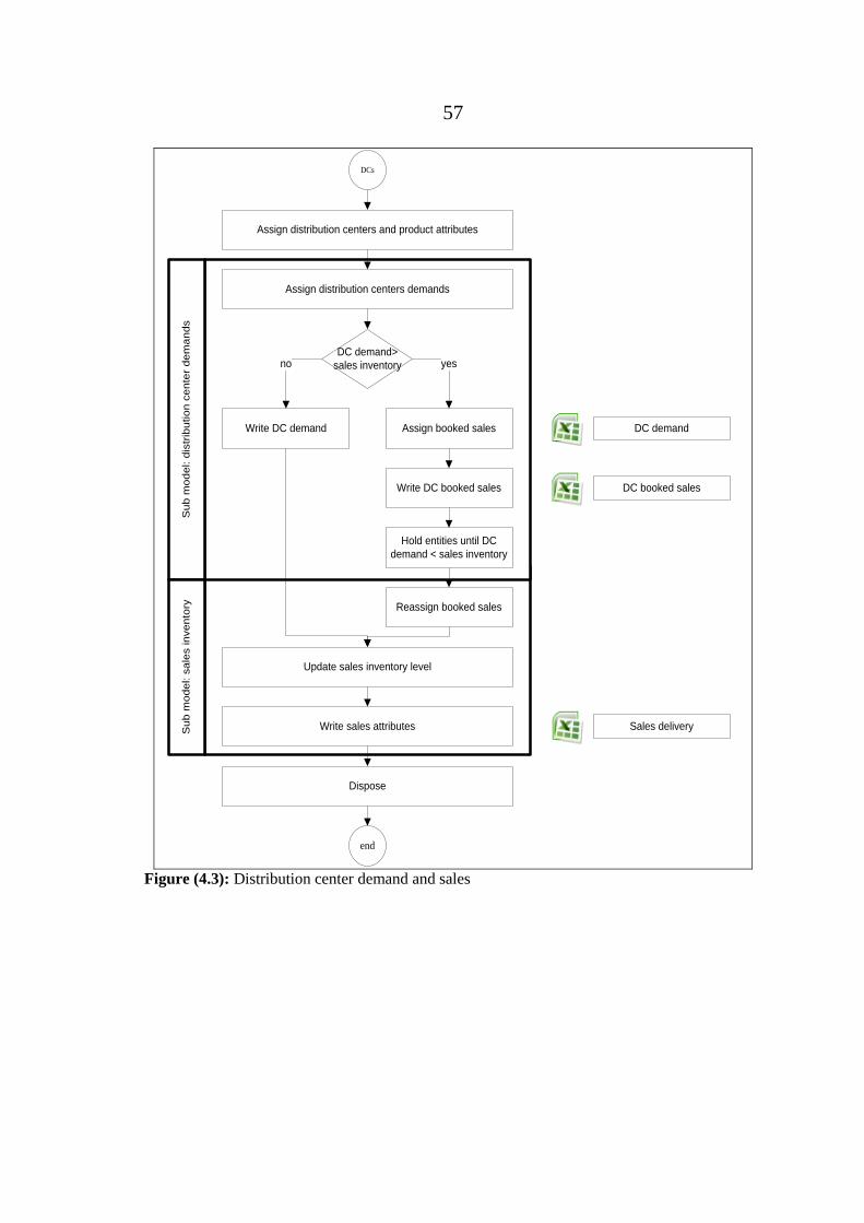
57

DCs

Assign distribution centers and product attributes

Assign distribution centers demands

DC demand>

sales inventory

Assign booked sales

yes

Write DC demand

no

Write DC booked sales

Hold entities until DC

demand < sales inventory

Reassign booked sales

Update sales inventory level

Write sales attributes

Dispose

end

DC demand

DC booked sales

Sales delivery

Su

b m

od

el: d

istr

ibu

tio

n c

en

ter

de

ma

nd

sS

ub

mo

de

l: s

ale

s in

ve

nto

ry

Figure (4.3): Distribution center demand and sales

58

Expected production quantity for each managed production order is

assigned as in EQ.12.

For production period 1

EQ.12


Production orders enter sub-submodel named raw material inventory

planning to assign expected consumable raw material. The sub-submodel

checks the availability of them. If the raw material is not available, the

production fails and leaves the system after assigning lost producable

quantities.Then another production order bookes the available line.

Product sales invnetory shortage is the core player; the simulation model

check if the expected product quantity will fullfill the shortage.In case the

expected product quantity is enough and assigned consumable raw

materials are available, the production order will be assgned to be

produced in the first production period. so, the production line will be free

for the second production period and another production order can be

assigned to be produced in the second production period.

If the expected product quantitiy of the the first product will not fullfill the

shortage, the correspondent production line will be booked to produce the

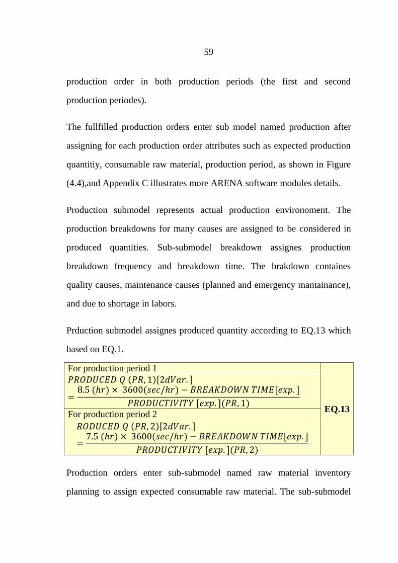
59

production order in both production periods (the first and second

production periodes).

The fullfilled production orders enter sub model named production after

assigning for each production order attributes such as expected production

quantitiy, consumable raw material, production period, as shown in Figure

(4.4),and Appendix C illustrates more ARENA software modules details.

Production submodel represents actual production environoment. The

production breakdowns for many causes are assigned to be considered in

produced quantities. Sub-submodel breakdown assignes production

breakdown frequency and breakdown time. The brakdown containes

quality causes, maintenance causes (planned and emergency mantainance),

and due to shortage in labors.

Prduction submodel assignes produced quantity according to EQ.13 which

based on EQ.1.


EQ.13


Production orders enter sub-submodel named raw material inventory

planning to assign expected consumable raw material. The sub-submodel

60

checks the availability of them. If the raw material is not available, the

production order fails and leaves the system after assign lost produced

quantities.Then another production order does not book the available line

and the lost production quantitiy is described as cost.

Although production orders leave the system but their attributes and

variables are transmitted and expressed to the second model by using Excel

sheets. The Attributes include day creation, product, deliverable product

pallets, distination distribution center, and delivery time (day). Number of

product delliverable pallets is calculated as in EQ.14.

EQ.14

The last type of created orders in this simulation model is raw material

orders, which enter raw materiall station. Raw material management

modules check if the order frequency (periodic raw material order) and

assgne there ordered quantities, as shown in Figure (4.5), and Appendix C

illustrates more ARENA software modules details.

As soon as the raw material ordered quantities are assigned, the simulation

update raw material inventory level as in EQ.15.

EQ.15

61

Assign production attributes (product, production line, total booked sales)

Assign products priority (hold until all products orders enter the sub model)

If sales

shortage > 0

yes

Su

b m

od

el:

pro

du

ctio

n m

an

ag

em

en

t

Production

lines

if production lines

availability (1st and

2nd

periods)

Assign only one product and production

quantity (second period)

Assign only one product and production

quantity (first period)

If product

group =2

no

Chang product group 2 to 1

yes

Check

production line

1 availability

Production line

for period 2

is available

No

Production line

for period 1

is available

Production

line for

period 1

is available

Production

line for

period 2

is available

No

A

Dispose

end

Figure (4.4): Sub-Model: Production Management (Continue)

62

Su

b-

su

b m

od

el: r

aw

ma

teria

l in

ve

nto

ry p

lan

nin

g

Dispose

end

Lost planning Rm

Su

b m

od

el: p

rod

uctio

n m

an

ag

em

en

t

Assign first raw material

If raw material

≤11No

Assign consumable raw material

Yes

If consumable raw

material ≤ raw

material inventory

Assign next raw materialCheck raw material

iterations until =1

Yes No

Reassign consumable raw

material (booked raw

material)

NO

Check production

periods

Yes

Assign lost expected

production due to raw

material for 1st & 2

nd

periods



material for 1st period



material for 2nd

period

Period=1 & 2

Period =2

Period =1

Write lost production due to raw material

Check if sales

inventory shortage<

expected pr

quantities

Assign production line 2=0

and expected production

quantities for 1st & 2

nd periods

No

Check production

period

Yes

Assign expected production


nd

periods

Assign expected

production quantities for

1st period

Assign expected production

quantities for 2nd

period

Period= 2

Period= 1& 2Period =1

Write EXPECTED PRODUCTION

A

B

Figure(4.4):Sub-Model: Production Management (Continue(

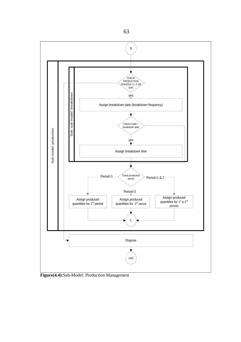
63

Su

b m

od

el: p

rod

uctio

n

Su

b-

su

b m

od

el: b

rea

kd

ow

n

CHECK

PRODUCTION

PERIODS =1, 2 OR

both

Assign breakdown date (breakdown frequency)

yes

Check if date =

breakdown date

Assign breakdown time

yes

Check production

period

Assign produced


nd

periods

Assign produced

quantities for 1st period

Assign produced

quantities for 2nd period

Period=1

Period=2

Period=1 & 2

B

C

Dispose

end

Figure(4.4):Sub-Model: Production Management

64

Dispose

end

Assign sales inventory and write produced quantities and lost quantities

Lost planning Rm

Su

b-

su

b m

od

el: r

aw

ma

teria

l in

ve

nto

ry p

lan

nin

g

Assign first raw material

If raw material

≤11

Assign consumable raw material

Yes

If consumable raw

material ≤ raw

material inventory

Assign next raw materialCheck raw material

iterations until =1

Yes No

Reassign consumable raw

material (booked raw

material)

NO

Check production

periods

Yes



material for 1st & 2

nd

periods



material for 1st period



material for 2nd

period

Period=1 & 2

Period =2

Period =1

Write lost production due to raw material shortage

no

Su

b m

od

el: p

rod

uctio

n

C

PRODUCED Q

Figure(4.5):Raw material orders (Continue (

65

Raw

material

Check if date =

order

frequency date

yes

no Assign raw material inventory = raw material inventory+

ordered raw material

Assign available raw material =raw material inventory

Write ordered raw material

end

Dispose

ordered raw material

Figure(4.5):Raw Material order

All output data are expressed to “Sinokrot Sales Delivery simulation” by

MS EXCEL sheets named “Main Sinkort Model” as input data to “Sinokrot

Sales Delivery simulation” model.

“Sinokrot Sales Delivery simulation” is composed of 2 branches named;

delivery management and distribution management. Each of them creates

orders named delivery orders and distribution orders, as shown in Figure

(4.6), Appendix C shows more details.

66

START

Create Entities

Entity: orders

110 0rders per day

Assign Order Attributes and sequence

Route Entities

DELIVE

RYSALES

Figure(4.6): Create entities and orders (Sinokrot Sales Delivery simulation)

When delivery orders are created (100 entity per working day), they assign

required attributes such as day, month, distribution center, and deliverable

pallets. The orders are grouped until deliverable pallet exceeds half pallet

for each product that will be delivered. After that, products delivery orders

are grouped until total deliverable pallets exceeds 10 pallets and not more

than 12 pallets. Next, the simulation model assigns charge ready for

distribution. Otherwise, when product delivery pallets is less than half

pallet, they booked until exceeds half pallet. As shown in Figure (4.7).

Distribution orders are created to represent charges, i.e. number of

distribution orders is same as number of charges as output of delivery

management. The distributions orders wait until transporters are available,

67

then they are transported to specified distribution center and recording

waiting and transportation time, as shown in Figure (4.8).

Sales

Read sales attributes

(day, PR, DC, deliverable product pallet, to-delivery time)

Assign sales delivery attributes and rounding to 0.25 pallet

Deliverable

pallets >= 0.5yes

no

Assign DC deliverable

pallets

Dispose

end

Sales delivery

Assign small pallets

Deliverable

pallets < 12

Small pallets >

0.5

YesYes

Assign transportable DC pallets

No

No

Figure (4.7): Delivery management

68

start

Create distribution order = charges

Assign DC charging attributes

Transportation to attended DC

end

Sinokrot distribution

Hold distribution orders until availability of transporters

Write transportation attributes

Assign waiting time and transportation time

Figure (4.8): Distribution management

69

4.5. MODEL VERIFICATION

Verification is the process of insuring that the model operates as intended.

This phase generally consists of debugging. The following techniques are

used to perform debugging according to [Law and Kelton, 2000]:

4.5.1 DIVIDE AND CONQURE APPROACH

It is breaking the larger detailed system model into a smaller, simpler, or

perhaps higher-level model. Therefore, any errors in syntax or variable

naming can be more easily addressed to enhance the details or expansion of

the model.

SINOKROT simulation model is divided to two main models; SINOKROT

main model and SINOKROT delivery model related to each other by MS

EXCEL sheet to transfer data as shown in the following Figure (4.9).

4.5.2 ANIMATION

Different entity pictures

Entities pictures are not only used to show entities type but also the status

in the system as shown in Table (4.3).Some examples are shown in Figure

(4.10).To illustrate this concept, pictures of production entities are blue

pages to represent production orders for period 1, green pages to rep-resent

production orders for period 2, and red pages to represent failed production

orders..

70

SINOKROT SIMULATION MODEL

MAIN SINOKROT MODEL SINOKROT SALES DELIVERY

DISTRIBUTION

CENTERS

PRODUCTION

MANAGMENT

RAW MATERIAL

MANAGMENT

SALES DELIVERY

MANAGMENT

SALES

DISTRIBUTION

MANAGMENT

DEMAND

SALES

IVENTORY

PRODUCTION

MANAGMENT

PRODUCTION

RAW

MATERIAL

PLANNING

PRODUCTION

BREAKDOWNS

RAW

MATERIAL

CONSUMING

SIMULATION EXPANSION

SIMULATION

DETAILS

MODELS

SUBMODELS

AND SUB-

SUBMODELS

Figure (4.9): Simulation model structure for verification

Figure (4.10): Simulation entity type and picture for verification

71

Table (4.3): Simulation entity type and picture

Model Entity type Entity status Picture

SINOKROT

MAIN

MODEL

Demand and

sales entities

Sales demand order Yellow ball

Sales order Green ball

Booked sales order Red ball

Production

entities

Plan production order Envelope

Production order for

period 1 Blue page


period 2 Green page


both period Yellow page

Failed production order Red page

Raw material

entities

Raw material Empty box

Ordered raw material Package

SINOKROT

DELIVERY

MODEL

Delivery order

Delivery order Blue page

Pallets more than 0.5 Yellow page

Delivered pallets Empty box

Distribution

order

Distribution order Report

Transportation order Truck

Following or tracking the entities through the system, as shown in

Figure (4.11)

1. Using variable displays in the simulator screens, as shown in Figure

(4.12)

2. Stepping through the program

3. Writing data to external files, such as MS Excel sheets “Sinokrot

main model”.

4. Using error and debugs manger in ARENA Software, as shown in

Figure (4.13)

72

The final result of using previous verification techniques is that Sinokort

models of the case study are verified.

Figure (4.11): Following the entities for verification

73

Figure (4.12): Using variable displays for verification

Figure (4.13): Check the simulation model for verification

37

4.6 MODEL VALIDATION

There are two major types of validation according to [LAW and

Kelton,2000]:

“Face validity means that the model, at least on the surface,

represents reality, i.e. face validity is review the simulation results

for reasonableness, if the results are consistent with how the

74

enterprise perceives the system should operate, then the simulation

model is said to have face validity.

Statistical validity involves a quantitative comparison between the

output performance of the actual system and the model Sinokrot

simulation models are reviewed to assure face validation (reviewing

simulation results) by researcher and Sinokrot Staff. On the other

hand, statistical validity is conducted in the following manner

according to [Chung et al., 2004], and Figure (14.4) shows this

manner.

1. Analyzing statistically the real data and data that generated by

simulation model which named simulation data.

2. Check normality of real and simulation data by chi-square test,

Kolmogorov-Smirnov, or Anderson-Darling, with confidence

interval 95% in our case study (α = 0.05).

3. If both of them are normal distribution i.e. hypothesis test result is to

not reject the null hypothesis(as illustrated in General Concept of

Input Data Fitting in Appendix B), then natural pairing test must be

conducted, otherwise i.e. one of them is not normal distributed, non-

parametric test must be conducted.

4. T-student test is used to accept or reject the null hypothesis that both

of real data and simulation data are paired naturally. If result is not to

reject the null hypothesis, the simulation system is valid; otherwise,

75

if the result is to reject the null hypothesis, F-test must be conducted

to check if they have the same variances.

5. If both variances of both data are equal, then independent T-test must

be conducted, otherwise i.e. variances are not equal, Smith–

Satterthwaite test must be conducted.

6. If independent T-test shows no rejection of the null hypothesis, so

the simulation system is valid, otherwise the simulation model must

be developed and revalidated.

7. According to step 2, if one of them is not normal distributed, non-

parametric test should be conducted such as U test or rank sum test.

So if the result is to accept the null hypothesis, the simulation is

valid, and otherwise the simulation model must be developed and

revalidated.

8. According to step 5, if Smith–Satterthwaite test accept the null

hypothesis, simulation model is valid, otherwise, it must be

developed and revalidated.

To check the validity of Sinokrot simulation models, the real data and

simulation data are compared according the pervious procedure. Some of

these comparisons summaries are shown in Table (4.4) and Appendix D

shows the details.

It is concluded that Sinokrot simulation models are valid to the reality.

76

STARTBoth

Normal?Non-Parametric TestNo

Both Normal?

Yes

Natural Pairing?

Paired T-TestYes

Both Normal?

No

Vars Equal?Smith-Satterwaithe

TestNo

Yes Non-Parametric Test Finish

Figure (4.14): Simulation model validation procedure [Chung, 2004]

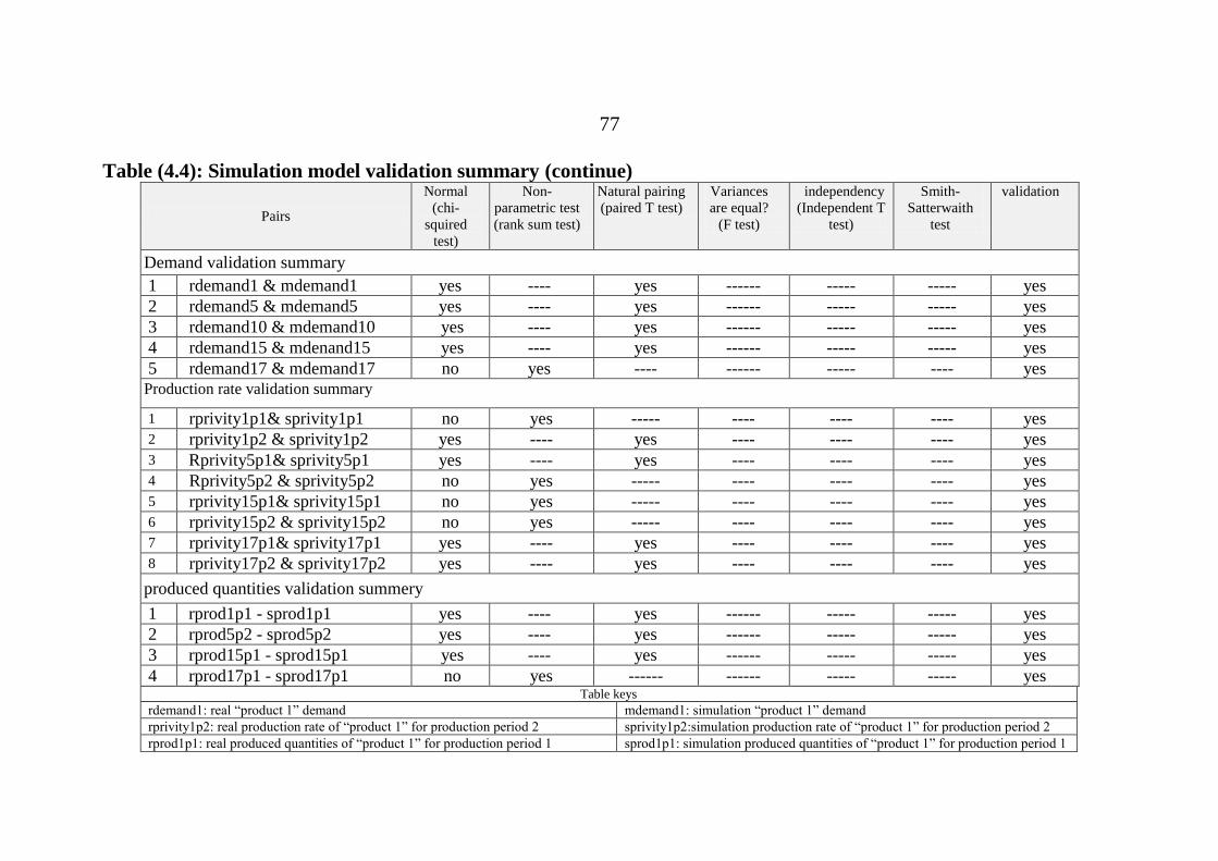
77

Table (4.4): Simulation model validation summary (continue)

Pairs

Normal

(chi-

squired

test)

Non-

parametric test

(rank sum test)

Natural pairing

(paired T test)

Variances

are equal?

(F test)

independency

(Independent T

test)

Smith-

Satterwaith

test

validation

Demand validation summary

1 rdemand1 & mdemand1 yes ---- yes ------ ----- ----- yes



4 rdemand15 & mdenand15 yes ---- yes ------ ----- ----- yes

5 rdemand17 & mdemand17 no yes ---- ------ ----- ---- yes

Production rate validation summary

1 rprivity1p1& sprivity1p1 no yes ----- ---- ---- ---- yes

2 rprivity1p2 & sprivity1p2 yes ---- yes ---- ---- ---- yes

3 Rprivity5p1& sprivity5p1 yes ---- yes ---- ---- ---- yes 4 Rprivity5p2 & sprivity5p2 no yes ----- ---- ---- ---- yes

5 rprivity15p1& sprivity15p1 no yes ----- ---- ---- ---- yes

6 rprivity15p2 & sprivity15p2 no yes ----- ---- ---- ---- yes

7 rprivity17p1& sprivity17p1 yes ---- yes ---- ---- ---- yes

8 rprivity17p2 & sprivity17p2 yes ---- yes ---- ---- ---- yes

produced quantities validation summery

1 rprod1p1 - sprod1p1 yes ---- yes ------ ----- ----- yes



4 rprod17p1 - sprod17p1 no yes ------ ------ ----- ----- yes Table keys

rdemand1: real “product 1” demand mdemand1: simulation “product 1” demand

rprivity1p2: real production rate of “product 1” for production period 2 sprivity1p2:simulation production rate of “product 1” for production period 2

rprod1p1: real produced quantities of “product 1” for production period 1 sprod1p1: simulation produced quantities of “product 1” for production period 1

78

4.7 REPLICATION EXPERIMENTALDESIGN

“The input distributions of simulation models are usually probabilistic in

nature. This input variability naturally results in some variation in the

output measures of performance. Because the output measures have some

variation, it is inappropriate for the simulation practitioner to recommend

any given course of action based on the results from a single simulation run

or replication. To reduce the chance of making a wrong recommendation, it

is necessary to run a number of simulation replications and then make the

recommendations based on all of the available data”. [Chung, 2004]

“A good design of simulation replications allows the analyst to obtain the

most statistical information from simulation runs for the least

computational cost. In particular, we seek to minimize the number of

replications and their length, and still obtain reliable statistics”. [Altiok et

al., 2007]

In our case, to obtain the minimum replications of Sinokrot simulation

model that assure reliable output statistics, simulation model variables such

as product sales are statistically studied and analyzed. “Product sales” as a

function of “number of replications” is shown in Figure (4.15) which

shows 12 replications as the minimum replication number.

79

Figure (4.15): Statistical steady state sales versus number of simulation replications

4.8 SCENARIOS DEVELOPMENT AND ANALYSIS

According to Dijk and Sluis,” Simulation is standard used and known for

evaluation purposes of process performance. Its application for

optimization purposes, however, seems to be limited mainly to a

comparison of scenarios or parameterized search methods”. [Dijk and

Sluis, 2008]

4.8.1 SCENARIO 1: 15% MARKET DEMAND INCREASE

OBJECTIVES

Study the effect of increasing in market demands upon the following

factors or variables:

1. Actual product sales

2. Product sales to product demand percentage

3. Daily sales inventory average

4. Produced quantities of products

5. Daily production lines utilization

700000

800000

900000

1000000

1100000

1200000

0 10 20 30 40 50 60 70

pro

du

ct 1

an

nu

al s

ale

s

number of simulation replications

80

6. Annual production line utilization

The last two performance variables can be defined as shown in EQ.16

and EQ.17. Where actual utilized production time during one period is net

production times after subtracting breakdowns times, and production time

is 8.5 hours for the first production period and 7.5 for the second

production period. While number of utilized production periods is annual

sumو first and second production periods are actually used. Number of

available production period is 624 production period per year (multiplying

of 2 production periods per day, 26 day per month, and 12 month per year).

EQ.16

Annual production line utilization

EQ.17

SCENARIO 1 RESULTS ANALYSIS AND

RECOMANDATIONS

Sinokrot simulation model is used to study the cited variables when market

demands of products increase by 15%. Those variables are compared with

ad hoc (as is) SFCo system. The comparison results are shown in Tables

4.4 and 4.5. While statistical experiment design are used to compare

population means such as T-test and F-test to compare statistically between

81

to populations, the results are not to reject null hypothesis (no differences

between the two populations) as shown in table (E.1) in appendix E.

Table (4.5) and Table (4.6) show the following points:

1. Sales to demand percentages are about 100% for both ad hoc and

scenario 1.

2. In general, annual produced quantities are the same in both systems.

To fulfill the 15% demand increase, Sales inventory level average

and inventory level at the end of year in scenario 1 are less than

those in ad hoc system.

3. Annual production line utilization percentages are the same for both

ad hoc and scenario 1to produce the same annual produced

quantities. It can be concluded that SFCo can fulfill the market

demand increase by 15 %.

Annual production lines results show weak annual utilization of production

lines. It is recommended to increase market demands of the products;

marketing campaigns must be increased in order to increase sales and

annual production line utilization.

82

Table (4.5): Scenario1 comparisons (15% demand increase), (continue)

Ad hoc (As is) system

PRODCUTS 1 2 3 4 5 6 7 8 9 10

Annual demand 1,396,993 9,889 124,535 213,019 87,219 122,756 15,548 13,348 6,699 9,959

Sales to demand % 100% 100% 100% 100% 100% 100% 100% 100% 100% 100%

Daily average of sales inventory 68,482 4,114 4,759 5,498 1,991 4,800 485 1,808 874 522

Sales inventory at end of year 75,283 2,468 4,668 5,512 1,871 4,322 522 3,066 333 880

Annual produced quantity 1,446,958 10,535 119,950 217,086 79,053 109,008 11,833 11,703 5,589 7,752 PRODCUTS 11 12 13 14 15 16 17 18 19 20

Annual demand 14,004 24,613 28,567 7,108 51,069 12,008 17,657 18,258 7,699 5,016

Sales to demand % 100% 100% 100% 100% 100% 98% 98% 100% 100% 99%

Daily average of sales inventory 569 1,604 1,444 450 3,628 1,550 2,047 1,476 836 952

Sales inventory at end of year 240 885 1,756 308 3,619 1,462 1,734 2,231 522 2,299

Annual produced quantity 10,787 21,080 22,868 5,684 49,501 11,638 15,874 16,955 6,315 6,666

Scenario 1 results

PRODCUTS 1 2 3 4 5 6 7 8 9 10

Annual demand 1,607,928 11,391 143,074 242,609 100,854 141,171 17,897 15,418 7,716 11,423

Sales to demand % 100% 100% 100% 100% 100% 100% 100% 100% 100% 100%


Sales inventory at end of year 56,152 16,342 2,686 37,323 2,474 5,104 484 1,391 1,286 452

Annual produced quantity 1,453,239 16,844 113,827 236,302 78,119 107,612 11,833 11,703 5,589 7,752 PRODCUTS 11 12 13 14 15 16 17 18 19 20

Annual demand 16,193 28,294 32,887 8,175 58,734 13,837 20,454 20,988 8,931 5,132

Sales to demand % 100% 100% 100% 100% 100% 98% 98% 100% 99% 100%


Sales inventory at end of year 300 1,896 1,210 525 3,572 2,556 2,531 966 730 2,552


83

Table (4.6): Production line utilization

DAILY PRODCUTION LINE UTILIZATION

PRODUCTION LINES 1 2 3 4 5 6 7 8

Ad hoc (As is) system 98.5% 99.2% 99.3% 98.3% 99.9% 99.9% 100.0% 100.0%

Scenario 1 results 98.6% 99.1% 99.2% 98.3% 99.9% 99.9% 100.0% 100.0%

ANNAUAL UTILIZATION OF PRODCUTION LINES

PRODUCTION LINES 1 2 3 4 5 6 7 8

Ad hoc (As is) system 48.6% 82.2% 10.6% 3.5% 8.7% 18.6% 4.6% 3.0%

Scenario 1 results 48.6% 82.4% 10.6% 3.5% 8.6% 18.6% 4.6% 3.0%

84

4.8.2 SCENARIO 2: DEVELOPMENT OF SALES INVENTORY

TARGET LEVEL

OBJECTIVES

Study the effect of reduction of sales inventory target on sales inventory

average.


RECOMANDATIONS

Production priority in Sinokrot simulation model is based on the

difference of product sales inventory target level and current product sales

inventory level. This deference is called product sales inventory shortage as

shown in EQ.2.

Scenario 2 based on the following questions, can sales inventory average

be reduced according to lean manufacturing philosophy? How can it be

done, and what are sales inventory target levels required in condition of

maintaining sales to demand percentages?

Sinokrot simulation model is used to determine minimum sales inventory

during the year and to determine scenario 2 sales targets as shown in

EQ.18.

Sales target level (scenario 2)

EQ.18

85

SCENARIO 2 RESULTS ANALYSIS AND RECOMANDATIONS

After running “scenario 2: simulation model”, the results are exhibited in

Table (4.7) and Table (4.8), and the following points can be concluded:

1. Reduction of sales target levels do not effect on the sales to demand

percentages and annual produced quantities.

2. Reduction of sales target levels lead to 83% sales inventory average

reduction, and- as a results- lead to reduction of inventory holding

cost.

3. Reduction decreases sales inventory at the end of year.

According to previous point, it is recommended to adopt the reduction of

sales targets.

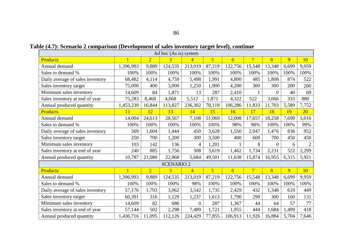
86

Table (4.7): Scenario 2 comparison (Development of sales inventory target level), continue Ad hoc (As is) system

Products 1 2 3 4 5 6 7 8 9 10

Annual demand 1,396,993 9,889 124,535 213,019 87,219 122,756 15,548 13,348 6,699 9,959

Sales to demand % 100% 100% 100% 100% 100% 100% 100% 100% 100% 100%


Sales inventory target 75,000 400 3,000 1,250 1,900 4,200 300 300 200 200

Minimum sales inventory 14,609 84 1,871 13 287 2,410 1 0 40 69

Sales inventory at end of year 75,283 8,468 4,668 5,512 1,871 4,322 522 3,066 333 880

Annual produced quantity 1,453,239 16,844 113,827 236,302 78,119 106,286 11,833 11,703 5,589 7,752

Products 11 12 13 14 15 16 17 18 19 20

Annual demand 14,004 24,613 28,567 7,108 51,069 12,008 17,657 18,258 7,699 5,016

Sales to demand % 100% 100% 100% 100% 100% 98% 98% 100% 100% 99%


Sales inventory target 250 700 1,200 300 3,500 400 600 700 450 450

Minimum sales inventory 103 142 136 4 1,201 1 8 0 6 2

Sales inventory at end of year 240 885 1,756 308 3,619 1,462 1,734 2,231 522 2,299


SCENARIO 2

Products 1 2 3 4 5 6 7 8 9 10

Annual demand 1,396,993 9,889 124,535 213,019 87,219 122,756 15,548 13,348 6,699 9,959

Sales to demand % 100% 100% 100% 98% 100% 100% 100% 100% 100% 100%


Sales inventory target 60,391 316 1,129 1,237 1,613 1,790 299 300 160 131

Minimum sales inventory 14,609 82 686 0 287 1,367 44 64 57 77

Sales inventory at end of year 57,144 502 2,298 7,489 1,721 1,955 444 1,684 1,499 418

Annual produced quantity 1,436,716 11,095 112,126 224,429 77,855 106,913 11,926 16,884 5,704 7,646

87

Table (4.7): Scenario 2 comparison (Development of sales inventory target level)

SCENARIO 2

Products 11 12 13 14 15 16 17 18 19 20

Annual demand 14,004 24,613 28,567 7,108 51,069 12,008 17,657 18,258 7,699 5,016

Sales to demand % 100% 100% 100% 100% 100% 98% 98% 100% 99% 100%

Daily average of sales inventory 365 1,948 1,337 441 2,456 1,547 1,843 1,473 1,027 866

Sales inventory target 147 558 1,064 296 2,299 399 592 700 444 448

Minimum sales inventory 94 213 136 4 1,266 2 9 611 109 2

Sales inventory at end of year 573 1,513 1,417 557 2,248 1,275 1,513 935 1,191 2,670


Table (4.8): Sales inventory average reduction

Products 1 2 3 4 5 6 7 8 9 10

Sales inventory average reduction 83% 44% 64% 64% 87% 51% 89% 75% 70% 86%

Products 11 12 13 14 15 16 17 18 19 20

Sales inventory average reduction 64% 121% 93% 98% 68% 100% 90% 100% 123% 91%

88

4.8.3 SCENARIO 3: ALLOCTING PRODCUTION LINE 1 FOR

PRODUCT GROUP 1 ONLY

OBJECTIVES

Study the effect of allocating production line 1 for product group 1

only upon the following variables:

Product sales to demand percentage

Annual produced quantities

Annual production line utilization


RECOMANDATIONS

Production line 1 is shared between product groups 1 and 2, while

production line 2 is allocated only for producing product group 2. In this

scenario, production line 1 is allocated to produce product group 1 only. To

study the effects of this scenario, Sinokrot simulation model is used after

deletion simulation modules that used to allow product group 2 enters the

production line 1 in production management sub-model.

After running “scenario 3 simulation model”, the results are exhibited in

Table (4.9) and Table (4.10), and the following points can be concluded:

Allocating “production line 1” to produce “product group 1” only does not

effect on sales to demand percentages. SFCo owns good potentials to

provide the market with same required products quantities.

Approximately, there are no differences between ad hoc system and

Scenario 3 in annual produced quantities.

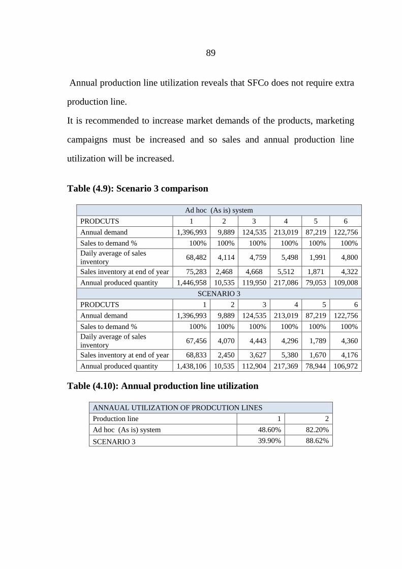
89

Annual production line utilization reveals that SFCo does not require extra

production line.

It is recommended to increase market demands of the products, marketing

campaigns must be increased and so sales and annual production line

utilization will be increased.

Table (4.9): Scenario 3 comparison

Ad hoc (As is) system

PRODCUTS 1 2 3 4 5 6

Annual demand 1,396,993 9,889 124,535 213,019 87,219 122,756

Sales to demand % 100% 100% 100% 100% 100% 100%

Daily average of sales

inventory 68,482 4,114 4,759 5,498 1,991 4,800

Sales inventory at end of year 75,283 2,468 4,668 5,512 1,871 4,322

Annual produced quantity 1,446,958 10,535 119,950 217,086 79,053 109,008

SCENARIO 3

PRODCUTS 1 2 3 4 5 6

Annual demand 1,396,993 9,889 124,535 213,019 87,219 122,756

Sales to demand % 100% 100% 100% 100% 100% 100%

Daily average of sales

inventory 67,456 4,070 4,443 4,296 1,789 4,360

Sales inventory at end of year 68,833 2,450 3,627 5,380 1,670 4,176

Annual produced quantity 1,438,106 10,535 112,904 217,369 78,944 106,972

Table (4.10): Annual production line utilization

ANNAUAL UTILIZATION OF PRODCUTION LINES

Production line 1 2

Ad hoc (As is) system 48.60% 82.20%

SCENARIO 3 39.90% 88.62%

90

4.8.4 SCENARIO 4: RAW MATERIAL INVENTORY MANGMENT

BASED ON FIXED-ORDERED QUANTITY

OBJECTIVES

Developing raw material inventory system based on simulation procedure

to:

1. Minimize average daily inventory level

2. Minimize inventory stock out to fulfill the production demand.

3. Determine optimum order quantity and optimum reorder point for

each raw material.

4. Analyze inventory attributes according to Lean manufacturing

philosophy, where Lean manufacturing is a management philosophy

focused on eliminating waste, reducing inventory, and increasing

profitability.

Ad hoc raw material inventory attributes, and performance variables are

shown in Table (4.11), note that costs are expressed by cost unit for

confidential purposes.

D. Blanchard mentions some principles that companies should follow to

build and manage lean systems as the following:

Measure any improvements in subsystem performance by weighing

their impact on the whole system.

91

Maintain inventories in an undifferentiated (unfinished) form for as

long as it is economically feasible to do so.

Buffer variation in demand with capacity, not inventory.

Use forecasts to plan and pull to execute.

Make decisions that promote a growth strategy and focus on

improving throughput.

Reduce variation in the system, which will allow the supply chain to

generate higher throughput with lower inventory and lower operating

expense.

SCENARIO 4 MODEL

There are many models that inventory management based on, but the

main models that widely used are fixed-ordered quantity model which will

be discussed here and fixed-time period model will be discussed in the

scenario 5. These models will be studied and analyzed by using simulation

techniques to achieve the objectives.

Total annual cost is sum of holding cost, annual demand, and ordering

cost. It can be calculated by EQ.19. Optimum order quantity can be

calculated by EQ.20 where is first derivative of EQ.19, and Figure (4.16)

illustrates optimum order quantity that minimize the total cost, while Figure

(4.17) shows the inventory position.

92

Figure (4.16): Annual Product cost, based on size

of order [Jacob and Chase, 2008]

Figure (4.17): Inventory position and lead time [Jacob and Chase, 2008]

Where: TC: Total annual cost D: demand (annual)

C: cost per unit Q: quantity to be ordered

S: cost of placing an order H: annual holding and storage cost per unit

L: lead time Z: number of standard deviations for a specified

service probability :average daily demand

R: Reorder point σL: standard deviation of usage during lead time

EQ.19

EQ.20

EQ.21

Safety stock = EQ.22

93

EQ.21 is applicable to determine re-order point when lead time is

deterministic and safety stock is considered according to standard deviation

of usage material during lead time. In reality, lead time is rarely

deterministic; however, it depends on dynamic variables such as logistics,

transportation, and administration arrangements. So there is more

probability of occurrence of risky stock out which leads to production

failures and increases costs and loses.

94

Table (4.11): Ad hoc raw material inventory system, continue

Raw material 1 2 3 4 5 6

Annual Demand (Kg) 799,509 521,615 297,669 627,633 3,861 27,105

Inventory Level Average (Kg) 45,705 38,746 30,128 54,849 1,163 2,236

Order Quantity (Kg) 45,000 49,000 32,000 62,000 1,000 2,600

Theoretical Optimum Order Quantity (Kg) 14,094 9,195 6,201 11,064 80 478

Number of Orders 24 12 12 12 12 12

Time between Orders (day) 13 26 26 26 26 26

Re-order Point (Kg) 43,562 23,700 15,456 33,024 362 848

Theoretical re-order point (Kg) 14,094 9,195 6,201 11,064 80 478

Stock-out probability 1.6% 4.4% 3.5% 2.6% 1.3% 1.1%

purchasing cost (per Kg) 4 4 3 5 15 11

Ordering Cost (per Order) 100 100 100 130 15 15

Holding Cost (per Kg) 0.60 0.60 0.60 0.60 1.00 0.80

purchasing cost (cost unit) 2,798,280 2,086,460 863,241 3,138,165 57,914 292,735

Ordering Cost (cost unit) 2,400 1,200 1,200 1,560 180 180

Holding Cost (cost unit) 27,423 23,248 18,077 32,910 1,163 1,789

Inventory Total Cost (cost unit) 2,828,103 2,110,908 882,518 3,172,634 59,257 294,704

95

Table (4.11): Ad hoc raw material inventory system

Raw material 7 8 9 10 11 Sum

Annual Demand (Kg) 46,088 236,163 15,816 908 25,994

Inventory Level Average (Kg) 5,986 20,156 4,630 35 4,930

Order Quantity (Kg) 5,800 23,500 3,900 200 4,300

Theoretical Optimum Order Quantity (Kg) 812 4,920 279 25 458

Number of Orders 12 12 12 3 12

Time between Orders (day) 26 26 26 100 26

Re-order Point (Kg) 2,668 22,391 1,072 81 2,281

Theoretical re-order point (Kg) 812 4,920 279 25 458

Stock-out probability 4.5% 2.2% 4.3% 19.4% 5.3%

purchasing cost (per Kg) 9 14 15 20 21

Ordering Cost (per Order) 38 100 60 10 40

Holding Cost (per Kg) 0.90 0.60 0.60 2.50 1.00

purchasing cost (cost unit) 396,359 3,235,430 234,073 18,166 545,864

Ordering Cost (cost unit) 456 1,200 720 31 480 13,666,687

Holding Cost (cost unit) 5,388 12,094 2,778 86 4,930 9,607

Inventory Total Cost (cost unit) 402,203 3,248,724 237,571 18,284 551,274 129,885

96

The following procedure is proposed to overcome the cited problem:

1. Run main Sinokrot simulation model, and collect the output file (excel

sheet named main Sinokrot simulation model) to obtained daily

demand of each raw material and total annual demand (D).

2. Determine the optimum order quantity theoretically by using equation

EQ.20.

3. Determine the mean of lead time statistical distribution, then consider

it as deterministic lead time then calculate Reorder point with safety

stock equals to zero.

4. Calculate theoretical Reorder point.

5. Build simulation model as shown conceptually in Figure (4.18) which

named scenario 4: fixed Q-based raw material inventory system, and

shown modularly in figure (E.1) in appendix E.

6. Tabulate values of multiplications of the optimum order quantity (Qopt)

and Reorder point for each raw material.

7. Run scenario 4 simulation models by using optimum order quantities

and reorder point as well as recording the results such as raw material

inventory, stock out percentage, and number of orders.

8. Calculate annual holding cost by using EQ.19 but take in

consideration that annual holding cost can theoretically calculated by

multiplying half of order quantity unit by holding cost per year. This

case is special case when stock out equals zero but practically it is

97

supposed to use raw material inventory level average instead of half

order quantity.

9. Calculate purchasing cost by multiplying cost per unit, order quantity

and number of orders.

10. Calculate ordering cost by multiplying cost per order by number of

orders.

11. Excel sheet is used to calculate the above costs and total annual

inventory costs are automatically calculated.

12. Re-run Scenario 4 simulation model by using multiplications of order

point and Reorder point values, and go through steps 7 to 12.

13. After complete the required table, sort Q values and Re-order point

values where inventory stock-out percentage greater than 0.

14. Actual optimum order quantity and optimum Re-order point where the

total costs are minimal as shown in Table (E.2) in appendix E.

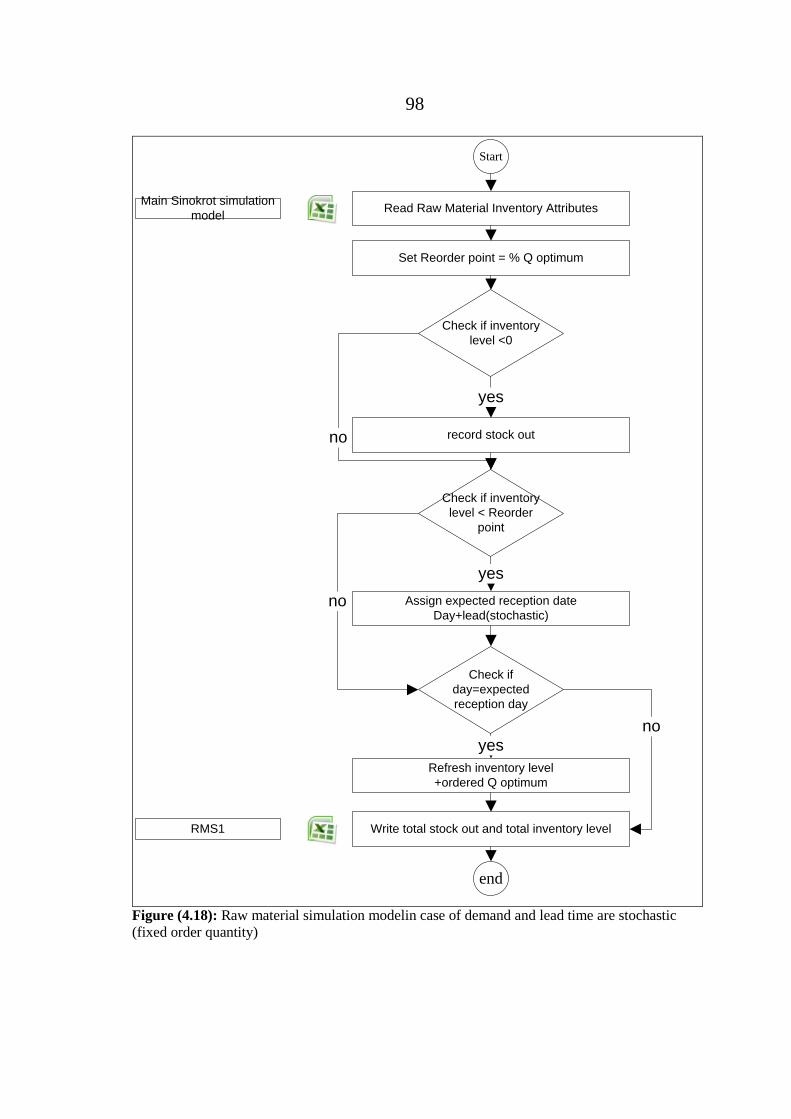
98

Start

Read Raw Material Inventory Attributes

record stock out

end

Refresh inventory level

+ordered Q optimum

Assign expected reception date

Day+lead(stochastic)

Main Sinokrot simulation

model

Check if inventory

level <0

yes

Check if inventory

level < Reorder

point

yes

Check if

day=expected

reception day

no

yes

Write total stock out and total inventory levelRMS1

Set Reorder point = % Q optimum

no

no

Figure (4.18): Raw material simulation modelin case of demand and lead time are stochastic

(fixed order quantity)

99

Table (4.12): Scenario 4 (Q-based inventory system, continue


Annual Demand (Kg) 652,068 421,354 242,371 324,455 2,206 24,197

Inventory Level Average (Kg) 151,787 50,443 40,590 162,938 1,316 1,905

Order Quantity (Kg) 130,414 105,338 80,790 324,455 2,206 4,033

Theoretical Optimum Order Quantity (Kg) 5 4 3 1 1 6

Number of Orders 64 80 107 320 320 53

Time between Orders (day) 105,704 9,195 6,201 11,064 80 478

Re-order Point (Kg) 0.0% 0.0% 0.0% 0.0% 0.0% 0.0%

Theoretical re-order point (Kg) 4 4 3 5 15 11

Stock-out probability 100 100 100 130 15 15

purchasing cost (per Kg) 0.60 0.60 0.60 0.60 1.00 0.80

Ordering Cost (per Order) 2,282,238 1,685,416 702,876 1,622,275 33,090 261,328

Holding Cost (per Kg) 500 400 300 130 15 90

purchasing cost (cost unit) 91,072 30,266 24,354 97,763 1,316 1,524

Ordering Cost (cost unit) 2,373,810 1,716,082 727,530 1,720,168 34,421 262,942


Inventory Total Cost (cost unit) 151,787 50,443 40,590 162,938 1,316 1,905

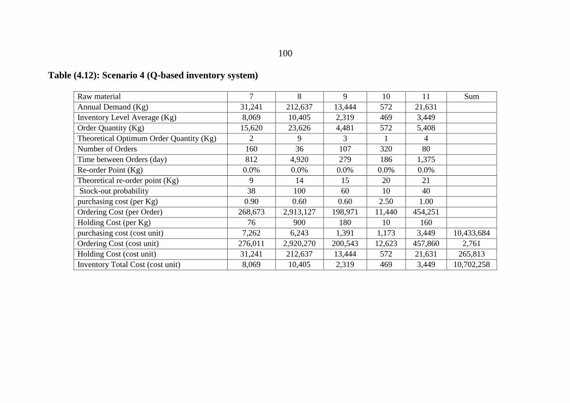
100

Table (4.12): Scenario 4 (Q-based inventory system)


Annual Demand (Kg) 31,241 212,637 13,444 572 21,631


Order Quantity (Kg) 15,620 23,626 4,481 572 5,408

Theoretical Optimum Order Quantity (Kg) 2 9 3 1 4


Time between Orders (day) 812 4,920 279 186 1,375

Re-order Point (Kg) 0.0% 0.0% 0.0% 0.0% 0.0%

Theoretical re-order point (Kg) 9 14 15 20 21

Stock-out probability 38 100 60 10 40

purchasing cost (per Kg) 0.90 0.60 0.60 2.50 1.00

Ordering Cost (per Order) 268,673 2,913,127 198,971 11,440 454,251

Holding Cost (per Kg) 76 900 180 10 160

purchasing cost (cost unit) 7,262 6,243 1,391 1,173 3,449 10,433,684

Ordering Cost (cost unit) 276,011 2,920,270 200,543 12,623 457,860 2,761

Holding Cost (cost unit) 31,241 212,637 13,444 572 21,631 265,813

Inventory Total Cost (cost unit) 8,069 10,405 2,319 469 3,449 10,702,258

101

Table (4.13): Compared costs of scenario 4 with ad hoc system


Purchasing cost (cost unit) 82% 81% 81% 52% 57% 89%

Ordering Cost (cost unit) 21% 33% 25% 8% 8% 50%

Holding Cost (cost unit) 332% 130% 135% 297% 113% 85%

Inventory Total Cost (cost unit) 84% 81% 82% 54% 58% 89%






102

SCENARIO 4 RESULTS AND RECOMANDATIONS

Results of executing raw material simulation procedure such as optimum

order quantity, optimum reorder point, daily average inventory, and total

inventory are shown in Table (4.12). Comparisons between main Sinokrot

simulation model and scenario 4 are conducted as shown in Table (4.13).

Statistical experiments are used to compare between main Sinokrot

simulation model and scenario 4 (Q-based raw material inventory). Daily

inventory level results which are optioned from both simulation models

present two different populations. Independent T test and F test are used to

conduct the null hypothesis assure that there are significant differences

between both populations means as shown in table (E.3) in appendix E. and

also Figure (4.19) represents this differences.

Table (4.13) exhibits significant differences in annual purchasing cost and

total annual inventory cost between the models; these differences refer to

many factors such as following:

1. Optimum Order quantity in scenario 4 is 360% more than ad hoc

system but consider that stock out percentages are 0% in scenario 4,

This factor leads to increase sales inventory average, and –as a

results- 205% increasing of holding cost.

2. Although of increasing in optimum order quantities, number of

orders in scenario 4 is less than in ad hoc system i.e. 29% ordering

cost to ad hoc system, an –as a result- the annual purchased

103

quantities is less than ad hoc system i.e. 76% purchasing costs to ad

hoc system.

3. Total annual inventory costs in scenario 4 are 78% of ad hoc system.

So it is recommended to adopt scenario 4.

Figure (4. 19): Raw Material 4 Inventory for main Sinokrot and scenario 4 models (raw

material 9)

0

1,000

2,000

3,000

4,000

5,000

6,000

7,000

8,000

1

12

23

34

45

56

67

78

89

10

0

11

1

12

2

13

3

14

4

15

5

16

6

17

7

18

8

19

9

21

0

22

1

23

2

24

3

25

4

26

5

27

6

28

7

29

8

30

9

Ram material 9 inventory level

ad hock scenario 4

104

4.8.5 SCENARIO 5: RAW MATERIAL INVENTORY MANGMENT

BASED ON FIXED-TIME PERIOD MODEL

OBJECTIVES

Developing raw material inventory system based on simulation procedure

in order to:

1. Minimize average daily inventory level.

2. Minimize inventory stock out to fulfill the production demand.

3. Determine optimum time between orders for each raw material.

4. Analyze inventory attributes according to Lean manufacturing

philosophy.

SCENARIO 5 MODEL

In fixed–time period system, inventory is counted only at particular

times, such as every week or every month. Also, generated order quantities

vary from period to period depending on the usage rates. Safety stock must

protect against stock outs during the review period itself as well as during

the lead time from order placement to order receipt.

Time between inventory reviews and putting orders (T) is determined by

inventory manger experience or routine visits of vendors taking in account

the ordered quantities have to fulfill raw material demands including time

between reviews and lead time as in EQ. 23.

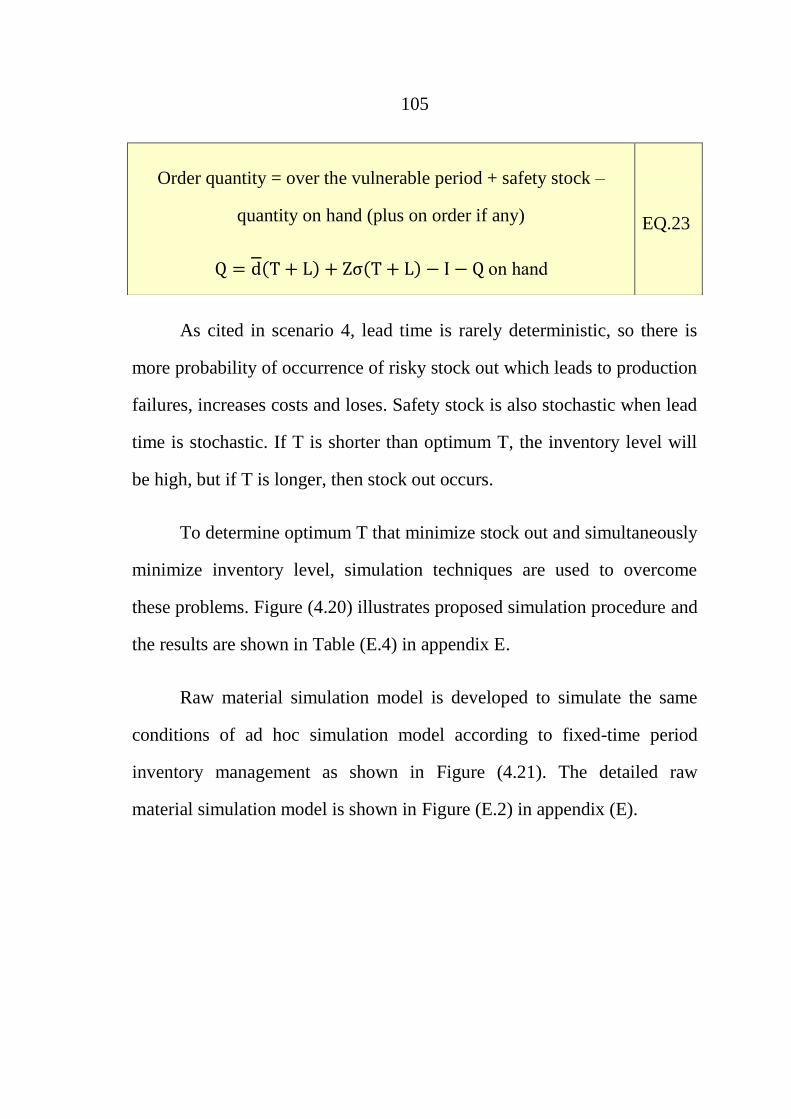
105

As cited in scenario 4, lead time is rarely deterministic, so there is

more probability of occurrence of risky stock out which leads to production

failures, increases costs and loses. Safety stock is also stochastic when lead

time is stochastic. If T is shorter than optimum T, the inventory level will

be high, but if T is longer, then stock out occurs.

To determine optimum T that minimize stock out and simultaneously

minimize inventory level, simulation techniques are used to overcome

these problems. Figure (4.20) illustrates proposed simulation procedure and

the results are shown in Table (E.4) in appendix E.

Raw material simulation model is developed to simulate the same

conditions of ad hoc simulation model according to fixed-time period

inventory management as shown in Figure (4.21). The detailed raw

material simulation model is shown in Figure (E.2) in appendix (E).

on hand

Order quantity = over the vulnerable period + safety stock –

quantity on hand (plus on order if any) EQ.23

106

Figure (4.20): Proposed simulation model of fixed time based raw material inventory

Run main (Sinokrot) simulation model

Collect raw material demand and inventory level

Build raw material simulation model

Assign T for all rawmaterials

Run raw material simulation model

Collect stock out, ordered quantities, and raw material inventory level

Set stock out occurrence probabilities (service level 100%)

Calculate total annual cost for each raw material for each T

Optimum T when percentage stock out-inventories ≤ service level and

minimum total annual cost

Reassign new T (until all Ts under study are assigned)

Develop main (Sinokrot) simulation model and run it

Conduct experimental design to compare developed performance indicators

with original performance indicators

107

Start

Read Raw Material Inventory Attributes

record stock out

end

Refresh inventory level

By adding ordered Q optimum

Assign expected reception date

day +lead(stochastic) and order Quantity

Sinokrot distribution

Check if inventory

level <0

yes

Check if day = T

yes

Check if

day=expected

reception day

no

Write total stock out, total inventory level, and

ordered quantitiesRMS2OUT

Set fixed-time periods T (day)

no

Tabulate T , total annual cost, set T optimum

that produces stock out probabilities less than

service level (0.05%) and minimizes total cost

Redevelop main simulation model, study and

analysis

Figure (4.21): Raw material simulation modelin case of stochastic demand andstochastic lead

time

108

Results of executing raw material simulation procedure such as order

quantity, optimum fixed-time period, daily average inventory, and total

inventory are shown in Table (4.14), while Table (4.15) exhibits

comparative results between ad hoc system and scenario 5(fixed-period-

based raw material inventory). Figure (4.22) presents inventory level of

“raw material 9” as an example in both models.

Moreover, Statistical experiments are used to compare between ad hoc

model and scenario 5. Daily inventory level results are optioned from both

simulation models present two different populations, T-test and F-test are

conducted as shown in table (E.5) in appendix E. it is assumed as a null

hypothesis there are mean differences between populations, where the

results assure that differences according to 95% confidence interval.

General results of Scenario 5 (T-based inventory system) exhibit the

following points:

1. Average of order quantities in this system is about 30% of order

quantities in the ad hoc system which leads to 67% reduction in

annual purchased quantities.

2. Ordering cost in scenario 5 is 117% when compared with ordering

cost in the ad hoc system due to number of orders in scenario 5.

3. When 67% reduction in annual purchased quantities occurs, the

holding cost is reduced to 81% due to reduction in average of raw

109

materials. This point clarifies how this system achieves lean

manufacturing objectives in reducing of inventories.

4. In general, total annual inventory cost drops to 67% of total annual

costs in the ad hoc system.

For the previous points, it is recommended that to adopt simulation

modeling of T-based inventory system, un-required stored quantities,

and total inventory costs must be reduced.

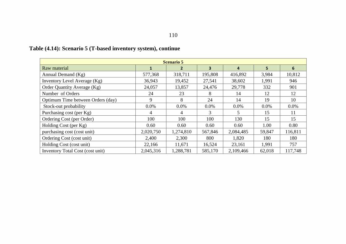
110

Table (4.14): Scenario 5 (T-based inventory system), continue

Scenario 5


Annual Demand (Kg) 577,368 318,711 195,808 416,892 3,984 10,812

Inventory Level Average (Kg) 36,943 19,452 27,541 38,602 1,991 946

Order Quantity Average (Kg) 24,057 13,857 24,476 29,778 332 901

Number of Orders 24 23 8 14 12 12

Optimum Time between Orders (day) 9 8 24 14 19 10

Stock-out probability 0.0% 0.0% 0.0% 0.0% 0.0% 0.0%

Purchasing cost (per Kg) 4 4 3 5 15 11

Ordering Cost (per Order) 100 100 100 130 15 15

Holding Cost (per Kg) 0.60 0.60 0.60 0.60 1.00 0.80

purchasing cost (cost unit) 2,020,750 1,274,810 567,846 2,084,485 59,847 116,811

Ordering Cost (cost unit) 2,400 2,300 800 1,820 180 180

Holding Cost (cost unit) 22,166 11,671 16,524 23,161 1,991 757

Inventory Total Cost (cost unit) 2,045,316 1,288,781 585,170 2,109,466 62,018 117,748

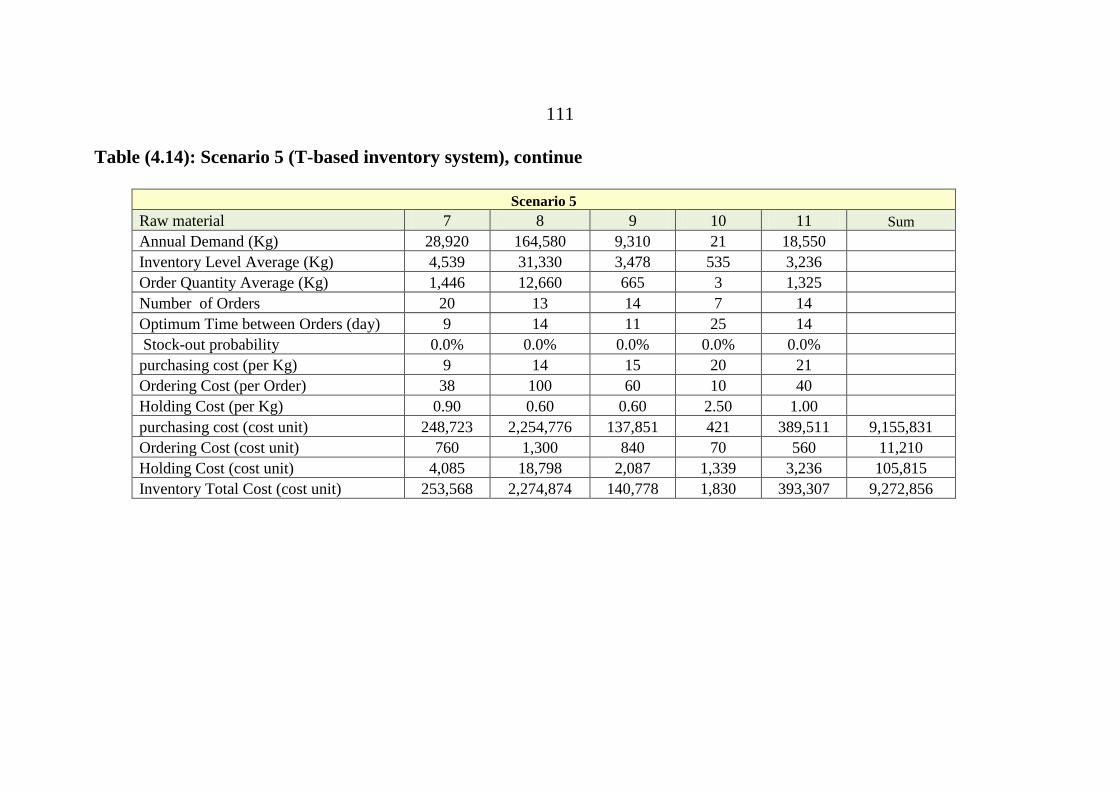
111

Table (4.14): Scenario 5 (T-based inventory system), continue

Scenario 5


Annual Demand (Kg) 28,920 164,580 9,310 21 18,550


Order Quantity Average (Kg) 1,446 12,660 665 3 1,325


Optimum Time between Orders (day) 9 14 11 25 14

Stock-out probability 0.0% 0.0% 0.0% 0.0% 0.0%

purchasing cost (per Kg) 9 14 15 20 21

Ordering Cost (per Order) 38 100 60 10 40

Holding Cost (per Kg) 0.90 0.60 0.60 2.50 1.00

purchasing cost (cost unit) 248,723 2,254,776 137,851 421 389,511 9,155,831

Ordering Cost (cost unit) 760 1,300 840 70 560 11,210


Inventory Total Cost (cost unit) 253,568 2,274,874 140,778 1,830 393,307 9,272,856

112

Table (4.15): Compared total inventory costs (scenario 5) with Ad hoc system






Order quantity (Kg) 53% 28% 76% 48% 33% 35%

Number of orders 185% 88% 31% 54% 46% 46%




Number of orders 77% 50% 54% 7% 54% 77%



Order quantity (Kg) 25% 54% 17% 2% 31%

113

Figure (4. 22): Raw Material 4 Inventory for main Sinokrot and scenario 5 model

0

2,000

4,000

6,000

8,000

1

15

29

43

57

71

85

99

11

3

12

7

14

1

15

5

16

9

18

3

19

7

21

1

22

5

23

9

25

3

26

7

28

1

29

5

30

9

ad hock

scenario 5

114

CHAPTER 5

THESIS CONCLUSION

5.1 THESIS RESULTS AND CONCLUSIONS

In this thesis, it is provided an overview of the main concepts that are

related to the simulation studies of supply chain management systems,

manufacturing system, and risk management. Simulation has the ability to

tell how a supply chain or a manufacturing system performs behave over

time when different rules and policies are applied. This point agrees with

conclusions at [Chang et al., 2002], [Thierry et al., 2010] and [Hennet et

al., 2009].

Simulation is used to study stochastic natures of demand, and lead time,

effect of finite production capacity over the performance of supply chain as

conducted in simulation scenarios. Like similar conclusions are conducted

in [Thierry et al., 2010] and [Cannella et al., 2008].

Simulation is a very efficient way of analyzing what – if scenarios and

can be used for improving the performance of manufacturing system i.e.

management and processes. The models were tested for many different

parameters. It would be beneficial to run a real life model on simulator

designed for those conditions before actual collaboration and decision

variable is put into practice.

115

Simulation models of a supply chain have been built to facilitate the use

of simulation in designing, evaluating, and optimizing supply chains. Some

Simulation models are discussed in this thesis. The first application is to

show behavior of supply chain, manufacturing, and risk attributes when the

market demand of products increases where the market demand is

stochastic variable. Also production rates and breakdowns are stochastic,

besides of interrelated variables such as consumed raw material (bill of

materials), and production lines readiness for production. Many

performance variables are considered in making decision such as sales to

demand percentage, produced quantities, daily production line utilization,

and annual production line utilization.

Simulation modeling detects behavior of the studied system and shows

performance variables so that enable mangers to take decisions at all levels;

for example, strategic decisions as focus marketing campaigns to increase

products sales. Also, there are operational decisions such as redesign

inventory target levels of products in order to increase production priorities.

And finally, the tactical decisions such as scheduling maintenance

(breakdowns reduction) in order to increase daily production line

utilization. In addition, the last point agrees with some pervious

conclusions which were cited in [Sun et al., 2009] and [Hübl et al, 2011].

Some simulation models are built to optimize inventory management;

either optimum order quantity based inventory management, or fixed time

reviewing based inventory management. These models are used when the

116

demand and supplier lead time are stochastic with complex interrelated

variable such as demand based on bill of materials of all products.

Simulation techniques are used to optimize order quantity and reorder

level (point) that minimize total inventory cost, minimize stored quantity

average or constrained with inventory capacity and in condition no stock-

out quantities. Simulation modeling of this inventory management show

reduction of annual cost and stored quantities average in absences of stock

out quantities.

On the other hand, simulation modeling of fixed time reviewing based

inventory to optimize the fixed time (T) that minimize total inventory cost,

reduce stored quantities average with stock-out probability equal to 0 i.e.

100% service level, and also, results show optimum fixed time that full fill

the cited parameters.

The last three conclusion points are similar to conclusions in [Alizadeh

et al., 2011] and [Alizadeh et al., 2011], but -in addition to stochastic

demand- the cited models in this thesis are based on stochastic produced

quantities, stochastic breakdowns, and integrated with production planning

models.

5.2 CONTRIBUTION TO KNOWLEDG AND PRACTICE

1. Developing integrated simulation system includes supply chain,

manufacturing, and risk application where:

117

Stochastic market demands of the products varies from month to

month, some of them follow trends where others do not, besides to

geographical distributed demands according to distribution centers.

Stochastic production rates depend on nature of products, stochastic

breakdowns frequency, stochastic breakdowns times, and production

periods.

Arranging soled products to nearest 0.25 pallets and arranging them

in order to maximize soled products according to transporter

capacity, in addition to checking available transporter.

Complex bill of material; where 11 raw materials are used in

production of 20 products i.e. used raw materials are interrelated

relations and combination of products.

Manufacturing system includes two models; production planning and

production process. Production planning is to check product priority,

available production line, expected producible quantity, expected

consumed raw material according to each product, and raw material

availability. Production process is to produce required product

quantities in both production period in consider breakdowns, raw

material availability, updates raw material inventory and sales (final

products) inventory.

Raw material inventory based on stochastic lead time and stochastic

raw material demands depend to stochastic demands of products.

118

2. Developing scenarios which are used to evaluate ad hoc system and

what if systems in order to improve product sales to product

demands, to increase annual production line utilization and to reduce

risk sales stock-out probabilities.

3. Developing optimization models in inventories management; fixed

order based inventory management and fixed reviewing period based

inventory management. These models are developed to determine

optimum order quantity and optimum reorder point that minimize

daily inventory management which minimize total annual inventory

cost with zero stock-out percentage. While the second one is to

determine optimum fixed reviewing period T to minimize daily

inventory management, minimize total annual inventory cost based

with zero stock out percentage. Both models are suitable for food

industry.

5.3 THESIS RECOMANDATIONS AND FUTURE WORKS

Besides to recommendations cited in scenarios, there are many future

works are recommended, either works based on current Sinokrot simulation

model, or works based on modified Sinokrot simulation models as the

following points:

Future works based on current simulation model include:

Studying and analyzing adopting optimum order quantity and reorder

point for the sales inventory (finished products) based in the same

119

method mentioned in scenario 4 to minimize risk of stock-out

percentages and total annual sales inventory cost.

Studying and analyzing adopting optimum reviewing time and

ordering for the sales inventory (finished products) based in the same

method mentioned in scenario 5.

Studying the manufacturing lead time to minimize sales inventory

stock-out percentage and total annual sales inventory costs.

Analyzing production rates of all production lines by adopting

polices to minimize breakdown times such as schedule maintenance

and minimize reworks to achieve Lean manufacturing philosophy.

Future works based on modified Sinokrot simulation models include:

Studying the negative effects of Israeli occupation obstacles in

delivering the finished products and/ or receiving raw materials. (It

can be based on situations occurred in 2002).

Studying the effect of fluctuated raw material prices on the whole

Sinokrot system.

Studying optimum geographical distribution of market distribution

centers i.e. number and sites, to minimize delivery costs, and

maximize Sinokrot market share.

Studying optimum allocating human resources (number of labors for

each production line) that maximize production rate, and minimize

the total production costs.

120

Adopt optimum manufacturing layout re-design that facilitate

production flows and minimize transportation.

Building a simulation model that facilitate production planning; so

that when production manager plan to next week, the excepted

produced quantity can be calculated based on the production

parameters such number of workers, expected break-downs, and

expected consumed raw materials, to facilitate also raw material

inventory to put an order or not.

121

REFERENCES

1. A. Akcay, B. Biller, and S. Tayur, 2012, A Simulation-based

Approach to Capturing Auto-correlated Demand Parameter

Uncertainty in Inventory Management, Proceedings of the 2012

Winter Simulation Conference, www.wsc.com..

2. A. Ali, X. Chen, Z. Yang, J. Lee and J. Ni, 2008, Optimized

Maintenance Design for Manufacturing Performance

Improvement Using Simulation, Proceedings of the 2008 Winter

Simulation Conference, www.wsc.com.

3. M. Alizadeh, H. Eskandari, and S. Sajadifar, 2011,Analyzing a

Stochastic Inventory System For Deteriorating Items with

Stochastic Lead Time Using Simulation Modeling, Proceedings of

the 2012 Winter Simulation Conference, www.wsc.com.

4. T. Altiok, and B. Melamed, 2007, Simulation Modeling and

Analysis with ARENA, 1st edition, Elsevier Inc., USA.

5. G. Altuger and C. Chassapis, 2009, Multi-Criteria Preventive

Maintenance Scheduling Through ARENA Based Simulation

Modeling, Proceedings of the 2009 Winter Simulation Conference,

www.wsc.com.

6. D. Axelson, P Gröndahl, A. Hägg, M. Jackson, K. Karlsson, M. Milic,

M. Sjöberg, and N. Tjärnberg, 2004, Woxen report, No. 36, ISSN

1650-1888.

http://www.wsc.com/

http://www.wsc.com/

http://www.wsc.com/

http://www.wsc.com/

122

7. S. Bangsow, 2010, Manufacturing Simulation with Plant

Simulation and SimTalk: Usage and Programming with Examples

and Solutions, Steffen Bangsow, p2.

8. M. Better, F. Glover, G. Kochenberger, and H. Wang, 2008,

Simulation optimization: Applications in Risk Management,

International Journal of Information Technology & Decision

Making, Vol. 7, No 4 (2008) 571-587.

9. B. Blanchard, 1991, System Engineering Management, John Willy

and Sons, New York.

10. D. Blanchard, Supply Chain Management: Best Practices, John

Wiley & Sons, Inc., Hoboken, New Jersey, 2007.

11. G. Booch, 1991, Object-Oriented Design with Applications, The

Benjamin /Cummings Publishing company, Inc., Redwood City,

CA.

12. J. Brown and D. Sturrock, 2009, Identifying Cost Reduction and

Performance Improvement: Opportunities through Simulation,

Proceedings of the 2009 Winter Simulation Conference,

www.wsc.com.

13. S .Cannella, E. Ciancimino and A. Márquez, Capacity constrained

supply chains: a simulation study, International Journal of

Simulation and Process Modeling, Vol. 4, No. 2, pp.139–147, 2008.

http://www.wsc.com/

123

14. Y. Chang and H. Makatsoris, 2002, Supply Chain modeling Using

Simulation, International Journal of SIMULATION Vol. 2 No. 1,

p24-30.

15. N. Chen and L. J. Hong, 2007, Monte Carlo Simulation in Financial

Engineering, Proceedings of the 2007 Winter Simulation

Conference, www.wsc.com

16. C. Chung, 2004, Simulation Modeling Handbook: a Practical

Approach,1st edition, CRC Press LLC, USA.

17. N. Dijk, and E. Sluis, 2008, Practical Optimization by OR and

Simulation, Simulation Modeling Practice and Theory, Elsevier

Inc.,www.elsevier.com.

18. E. Enrich, Oxford American Dictionary, Oxford University Press.

New York.

19. R. Flangagan, and G. Norman, 1999, Risk management and

construction, 4th edition, Black-well Ltd, United Kingdome.

20. M. Gregg, S. Van Andel, and S. Saylor, 2011, Lean+ Manufacturing

Process Analysis Simulation (LPAS+), Proceedings of the 2011

Winter Simulation Conference, www.wsc.com.

21. C. Grewal, S. Enns, and P. Rogers, 2009, Performance Effects of

Setup Time Reduced with and without Decision Variable Re-

Optimization: A simulation Optimization Study, Proceedings of

the 2009 Winter Simulation Conference,www.wsc.com.

http://www.wsc.com/

http://www.elsevier.com/

http://www.wsc.com/

http://www.wsc.com/

124

22. B. El- Haik and R. Al-Aomar, 2006, Simulation- Based Lean Six-

Sigma and Design for six-sigma, A John Wiley & Sons, Inc.,

Hoboken, New Jersey, USA.

23. C. Harrell, B. Ghosh, and R. Bowden, 2004, Simulation Using

ProModel,2nd edition, McGraw-Hill Companies, Inc.

24. J. Heilala, S. Vatanen, H. Tonteri, J. Montonen, S. Lind,B. Johansson,

and J. Stahre, 2008,Simulation–Based Sustainable Manufacturing

System Design, Proceedings of the 2008 Winter Simulation

Conference, www.wsc.com.

25. D. Hellström, and M. Johnsson. 2002. “Using Discrete-event

Simulation in Supply Chain Planning.” 14th

Annual Conference for

Nordic Researchers in Logistics. Trondheim, Norway: NOFOMA

26. J. Hennet, J. Mercantini, and I. Demongodin, 2009, Toward an

Integration of Risk Analysis in supply chain Assessment,

www.lsis.org.

27. A. Hübl, K. Altendorfer, H. Jodlbauer, M. Gansterer, R. F. Hartl,

2011, Flexible Model for Analyzing Production System With

Discrete Event Simulation, Proceedings of the 2011 Winter

Simulation Conference, www.wsc.com.

28. F. Jacob and R. Chase, 2008, Operations and Supply Management:

The Core, by McGraw-Hill/Irwin, New York.

http://www.wsc.com/

http://www.lsis.org/

http://www.wsc.com/

125

29. M. Kämpf and P. Köchel, 2006, Simulation-based sequencing and

lot size optimization for a production-and-inventory system with

multiple items, Elsevier Inc., www.elsevier.com.

30. WW. Kelton, RSadowski, and D. Sadowski, 2001, Simulation with

ARENA, 2nd edition, McGraw-Hill.

31. A. Law, and D. Kelton,. 2000, Simulation Modeling and Analysis,

3rd

edition, McGraw-Hill, New York.

32. V. Lesnevski, B. L. Nelson, and J. Staum, 2006, An Adaptive

Procedure Of estimating Coherent Risk Measures Based On

Generalized Scenarios, Proceedings of the 2006 Winter Simulation


33. A. Mahfouz, J. Shea, and A. Arisha, 2011, Simulation Based

Optimization Model for The Lean Assessment In SME: A Case

Study, Proceedings of the 2011 Winter Simulation Conference,

www.wsc.com.

34. G. Papageorgiou and A. Hadjis, 2011, Strategic Management via

System Dynamics Simulation Models, World Academy of Science,

Engineering and Technology 2011 , European University Cyprus,

Nicosia, Cyprus

35. P. Pawlewski and M. Fertsch, 2010, Modeling and Simulation

Method to Find and Eliminate Bottlenecks in Production Logistics

Systems, Proceedings of the 2010 Winter Simulation Conference,

www.wsc.com.

http://www.elsevier.com/

http://www.wsc.com/

http://www.wsc.com/

126

36. X. Qi, 2007, Order splitting with multiple capacitated suppliers’,

European Journal of Operational Research, Vol. 178, No. 2,

pp.421–432.

37. A. Samvedi and V. Jain, 2011,StudingThe Impact Of Various

Inventory Policies On A Supply Chain With Intermittent Supply

Distributions, Proceedings of the 2012 Winter Simulation


38. A. Saxena, Y. Ducq, R. Malairajan and P. Sivakumar,2010,

Simulation based Decision Making Scenarios in Dynamic Supply

Chain, International Journal of Enterprise Network Management

4, 2 (2010) 166-182.

39. S. Sengupta, K. Das, and R. VanTil, 2008, A New Method for

Bottleneck detection, Proceedings of the 2008 Winter Simulation


40. L. Sun, S. Heragu, L. Chen, and M. Spearman, 2009, Simulation

Analysis of a Multi-Item MRP System Based on Factorial Design,


www.wsc.com.

41. D. Tesfamariam, and K. Karlsson, 2005, a Systematic Analysis of a

Decision Making Process. Manufacturing Strategy and System

Configuration, Royal institute technology, Stockholm.

http://www.wsc.com/

http://www.wsc.com/

http://www.wsc.com/

127

42. C. Thierry, G. Bel and A. Thomas, 2010, The Role of Modeling and

Simulation in Supply Chain Management, Supply Chain

Management M&S Magazine – 2010 / n4 (Oct).

43. K. Vasudevan, R. Lote, E. Williams, and O. Ülgen, 2008, Iterative

Use of Simulation Scheduling Methodologies to Improve

Productivity, Proceedings of the 2008 Winter Simulation


44. D. Vose, 2000, Risk Analysis: A Quantitative Guide, John Wiley

and Sons, Chichester.

45. G. A. Wainer, 2009, Discrete-Event Modeling and Simulation: A

Practitioner’s Approach, CRC Press, Taylor & Francis Group,

USA.

46. K. White, and R. Ingalls, 2009, Introduction to Simulation,


p12:23.(2009-2)

47. L. Wilson, 2010, How to Implement Lean Manufacturing, The

McGraw-Hill Companies, Inc., New York, page 9.

48. T. Wu, L. Shi, B. Quirt, and N. Duffie, 2008, Integrated Dynamic

And Simulation Model on Coupled Closed-Loop Workstation

Capacity Controls in a Multi-Workstation Production System,


www.wsc.com.

49. B. Zandian, 2004, Maynard's Industrial engineering handbook,2nd

edition, McGraw Hill.

http://www.wsc.com/

http://www.wsc.com/

128

APPENDICES

APPENDIX A: CONCEPTUAL MODEL Table (A.1): Production lines and product groups

Production

Lines

Product

Groups

Products

1 1 Product 1,Product 2

2 (or 1*) 2 Product 3,Product 4, Product 5, Product 6

3 3 Product 7,Product 8, Product 9, Product 10

4 4 Product 11

5 5 Product 12, Product 13

6 6 Product 14, Product 15

7 7 Product 16, Product 17, Product 18

8 8 Product 19,product 20 * If “production line 1” is not busy

Table (A.2): Production Lines rates

Products Production Line Production rate (Second Per Case)

First Production Period Second Production Period

Product 1 **LOGN(4.5,0.48) LOGN(4.4,0.62)

Product 2 LOGN(6.3, 5.84) LOGN(5.5,7.91)

Product 3 LOGN(7.2, 1.83) LOGN(7.1, 1.4)

Product 4 LOGN(50.0,25.70) LOGN(48.62, 22.60)

Product 5 LOGN(52.7,20.96) LOGN(50.8, 4.30)










Product 15 LOGN(62.0, 8.40) LOGN(59.0,9.00)





Product20 LOGN(44.2, 20.00) LOGN(43.5, 22.30) ** LOGN(mu, sigma): Log Normal distribution

129

Table (A.3): General Production Line Breakdown

Production

Line

Breakdown Frequency

(Working Day)

Breakdown Time

(Second)

1 5 LOGN(4105, 713)

2 8 LOGN(4055, 510)

3 9 LOGN(4178, 450)

4 4 LOGN(4334, 409)

5 17 LOGN(910, 500)

6 11 LOGN(654, 330)

7 23 LOGN(1003, 640)

8 20 LOGN(1049,639)

Table (A.4): Raw Material Order Frequency, Ordered Quantities and

Reorder Point

Raw Material Order frequency

(production day)

Ordered

quantities (Kg)

Reorder point

(Kg)

Raw Material 1 13 47000 25000

Raw Material 2 26 49000 35000

Raw Material 3 26 32000 15000

Raw Material 4 26 52000 30000

Raw Material 5 26 1000 700



Raw Material 8 26 23500 12000


Raw Material 10 100 2000 2000

Raw Material 11 26 4300 15000

130

Table (A.5): Bill of Materials

Product Raw Materials (Kg)

1 2 3 4 5 6 7 8 9 10 11 Total

1 0.307 0.184 0.120 0.256 0 0.012 0.013 0.102 0 0 0.012 1.008

2 0.167 0.100 0.067 0.139 0 0.007 0.007 0.056 0 0 0.007 0.55

3 0.221 0.133 0.089 0.185 0 0.009 0.009 0.074 0 0 0 0.72

4 1.478 0.887 0.591 1.231 0 0.057 0.061 0.492 0 0 0 4.8

5 0.221 0.133 0.088 0.184 0 0.009 0.009 0.073 0 0 0 0.72

6 0.221 0.133 0.088 0.185 0 0.009 0.009 0.074 0 0 0 0.72

7 0.985 5.398 0 0.981 0 0.032 0 0 0.106 0 0 7.5

8 1.138 3.912 0 1.280 0 0.028 0 0.498 0.142 0 0 7

9 1.138 3.912 0 1.280 0 0.028 0 0.497 0.142 0 0 7

10 1.138 3.912 0 1.280 0 0.028 0 0.498 0.142 0 0 7

11 0.564 0 0.18 0 0 0 0.036 0 0 0 0.42 1.2

12 0.512 0 0.143 0 0 0.006 0.031 0 0 0 0.307 1

13 0.245 0 0.069 0 0 0.003 0.015 0 0 0 0.148 0.48

14 0.197 0.092 0.061 0.135 0.043 0 0.036 0.030 0.003 0 0 0.6

15 1.698 0.796 0.530 1.167 0 0 0.318 0.265 0.027 0 0 4.8

16 0.288 0 0.041 0.049 0 0.003 0.016 0.041 0.263 0 0.016 0.72

17 0.278 0 0.039 0.047 0.023 0.003 0.015 0.039 0.254 0 0.016 0.72

18 0.247 0 0.037 0.045 0.187 0 0.016 0 0.172 0 0.014 0.72

19 0.493 0 0 0.038 0 0 0 0 0.189 0 0 0.72

20 0.44 0 0 0 0 0 0 0 0.144 0.136 0 0.72

131

Table (A.6): Daily product demand statistical distributions

Product Daily Product Demand (case)

Month 1 Month 2 Month 3 Month 4 Month 5 Month 6

1 TRIA(4948,520

8,5468)

TRIA(4508,4745

,4982)

TRIA(4462,

4697, 4932)

TRIA(4578,

4819, 5060)

TRIA(3745,

3942, 4139)

TRIA(3779,

3978, 4177)

2 UNIF(40,55) UNIF(35, 39)

TRIA(17, 19,

20) UNIF(37, 41) UNIF(31, 35) UNIF(13,16)

3 TRIA(462,486,

510)

TRIA(517, 544,

571)

TRIA(300,

316, 332)

TRIA(353,

372,510)

TRIA(335,

353, 371)

TRIA(343, 361,

379)

4 TRIA(706, 743,

780)

TRIA(689, 725,

761)

TRIA(726,

764, 802)

TRIA(574,

604, 634)

TRIA(818,

861, 904)

TRIA(647, 681,

715)

5 TRIA(315, 332,

349)

TRIA(278, 293,

308)

TRIA(199,

209, 219)

TRIA(574,

604, 634)

TRIA(234,

246, 258)

TRIA(320, 337,

354)

6 TRIA(372,

390,400)

TRIA(411, 433,

455)

TRIA(390,

411, 432)

TRIA(311,

327, 343)

TRIA(449,

473, 497)

TRIA(486, 512,

538)

7 UNIF(30,40) UNIF(16, 18) UNIF(20, 22)

TRIA(25, 30,

37) UNIF(22, 25) UNIF(13,16)

8 UNIF(30,50) UNIF(55, 61) UNIF(36, 40) UNIF(28, 30) UNIF(31, 35)

TRIA(35, 37,

39)

9 UNIF(20,24) UNIF(28, 30) UNIF(15, 22) UNIF(13, 17) UNIF(18, 21) UNIF(17, 20)

10 UNIF(7,10)

TRIA(16, 17,

18) UNIF(10, 14) UNIF(20, 25) UNIF(36, 43) UNIF(20,23)

132

Table (A.6): Daily product demand statistical distributions (continue)



11 UNIF(50,70)

TRIA(107, 113,

119) UNIF(70, 90) UNIF(67, 75) UNIF(23, 27) 0

12 UNIF(86,95) UNIF(68, 76) UNIF(110, 122) UNIF(69, 77) UNIF(110, 122) TRIA(36, 38, 40)

13 TRIA(758, 798,

838)

TRIA(145, 153,

161) TRIA(143, 150, 158) UNIF(68, 77) UNIF(72, 80) TRIA(74, 78, 82)

14 UNIF(31, 35) UNIF(31, 35) UNIF(33, 37) TRIA(12, 14, 15) TRIA(5, 8, 9) UNIF(5,8)

15 UNIF(131, 145)

TRIA(161, 169,

177) TRIA(193, 203, 220) UNIF(100, 115) UNIF(72, 80) TRIA(108, 114, 120)

16 UNIF(48, 54) TRIA(66, 69, 72) TRIA(87, 94, 99) TRIA(11, 14, 16) TRIA(21, 22, 25) UNIF(0,5)

17 UNIF(127, 141)

TRIA(130, 137,

144) UNIF(30, 45) TRIA(65, 74, 76) TRIA(30, 32, 34) UNIF(28, 30)

18 0

TRIA(109, 115,

121) UNIF(170, 190) 0 UNIF(89, 100) UNIF(35, 39)

19 UNIF(49, 55) UNIF(65, 71) TRIA(20, 25, 27) UNIF(147, 167) UNIF(240, 266) UNIF(46, 50)

20 TRIA(14, 15, 16) UNIF(25, 27) UNIF(35, 39) TRIA(46, 50, 55) UNIF(109, 121) UNIF(72, 80)

133


Produc

t

Daily Product Demand (case)


1 TRIA(3663,

3856, 4049)

TRIA(3741,

3938, 4135)

TRIA(3700,

3895, 4090)

TRIA(4206,

4427, 4648)

TRIA(4485,

4721, 4957)

TRIA(5235,

5511, 5787)

2 UNIF(9,13)

TRIA(24, 25,

27) UNIF(30, 34) UNIF(35, 42) UNIF(43, 47) UNIF(37, 41)

3 TRIA(390,

411, 432)

TRIA(316,

333, 352)

TRIA(516,

543, 570)

TRIA(276,

290, 302)

TRIA(313,

329, 350)

TRIA(390,

411, 432)

4 TRIA(740,

779, 818)

TRIA(550,

586, 615)

TRIA(571,

601, 631)

TRIA(500,

526, 552)

TRIA(648,

682, 716)

TRIA(594,

625, 656)

5 TRIA(185,

195, 205)

TRIA(136,

143, 150)

TRIA(200,

210, 225)

TRIA(175,

184, 193)

TRIA(299,

315, 329)

TRIA(273,

287, 301)

6 TRIA(446,

469, 492)

TRIA(2631,

2769, 2907)

TRIA(371,

390, 410)

TRIA(353,

372, 391)

TRIA(314,

330, 347)

TRIA(383,

403, 423)

7 UNIF(35, 39) UNIF(52, 58) UNIF(71, 80) UNIF(85, 100)

TRIA(112,

118, 124) UNIF(70, 80)

8 TRIA(44, 46,

48)

TRIA(30, 33,

35)

TRIA(44, 46,

47)

TRIA(59, 62,

65) UNIF(48, 55)

TRIA(40, 42,

46)

9 UNIF(19, 21) UNIF(15, 20) UNIF(20, 23) UNIF(29, 35)

TRIA(22, 24,

25) UNIF(19, 23)

10 UNIF(12, 14) UNIF(23, 27) UNIF(28, 31) UNIF(35, 43) UNIF(68, 78) UNIF(78, 86)

134




11 0 0 UNIF(12, 15) UNIF(48, 53)

TRIA(48, 50,

54) UNIF(72, 80)

12 TRIA(38, 40,

42)

TRIA(70, 76,

80)

TRIA(112,

118, 126)

TRIA(76, 80,

84) UNIF(45, 55) UNIF(72, 80)

13 TRIA(75, 79,

83)

TRIA(39, 41,

43)

TRIA(52, 55,

58)

TRIA(52, 55,

58) UNIF(58, 64) UNIF(76, 84)

14 UNIF(4,7) UNIF(15,18) UNIF(20, 24) UNIF(20, 24) UNIF(43, 47) UNIF(30, 37)

15 TRIA(151,

159, 167)

UNIF(106,

118)

UNIF(205,

227)

UNIF(125,

139)

TRIA(242,

253, 269)

TRIA(265,

279, 295)

16 0 UNIF(10, 12) UNIF(32, 37) UNIF(28, 35) UNIF(35, 40) UNIF(74, 82)

17 UNIF(35, 39) 0

TRIA(15, 17,

18)

TRIA(65, 68,

71) UNIF(51, 55) UNIF(35, 39)

18 UNIF(31, 35) UNIF(23, 36) UNIF(31, 36) UNIF(20, 24) UNIF(73, 89) UNIF(72, 80)

19 UNIF(0, 3) 0 UNIF(2, 7) 0 0 0

20 UNIF(18, 22) UNIF(13, 17) 0 UNIF(2, 7) 0 UNIF(5, 8)

TRIA: Triangular Statistical Distribution (minimum value, average, maximum value)

UNIF: Uniform Statistical Distribution (minimum value, maximum value)

135

Table (A.7): Daily product demand of distribution center percentage

Product Distribution Center

1 2 3 4 5 Total

1 30.0% 30.0% 30.0% 10.0% 0.0% 100%

2 30.0% 30.0% 30.0% 10.0% 0.0% 100%

3 21.1% 15.8% 15.8% 36.8% 10.5% 100%

4 24.0% 24.0% 24.0% 28.0% 0.0% 100%

5 15.4% 0.0% 15.4% 15.4% 53.8% 100%

6 12.5% 25.0% 37.5% 25.0% 0.0% 100%

7 13.3% 6.7% 13.3% 46.7% 20.0% 100%

8 27.3% 27.3% 27.3% 18.1% 0.0% 100%

9 27.3% 27.3% 27.3% 18.1% 0.0% 100%

10 27.3% 18.2% 36.3% 18.2% 0.0% 100%

11 33.3% 11.1% 33.3% 22.3% 0.0% 100%

12 30.0% 20.0% 15.0% 5.0% 30.0% 100%

13 30.0% 20.0% 15.0% 5.0% 30.0% 100%

14 28.0% 28.0% 16.0% 20.0% 8.0% 100%

15 31.6% 26.3% 15.8% 10.5% 15.8% 100%

16 7.1% 14.3% 14.3% 35.7% 28.6% 100%

17 7.1% 14.3% 14.3% 35.7% 28.6% 100%

18 7.1% 14.3% 14.3% 35.7% 28.6% 100%

19 22.2 22.2 33.3 22.3 0 100%

20 22.2 22.2 33.3 22.3 0 100%

Table (A.8): Product Sales Target Level

Products Product Target

Level (case) Products

Product Target

Level (case)

Product 1 75,000 Product 11 250

Product 2 400 Product 12 750

Product 3 3,000 Product 13 1,200


Product 5 1,900 Product 15 3,500





Product 10 200 Product20 300

136

Table (A.9): Number of cases per pallet

Products Number of cases

per pallet Products

Number of cases

per pallet










Product 10 60 Product20 100

137

APPENDIX B: INPUT DATA FITTING (SAMPLES)

GENERAL CONCEPTOF INPUT DATA FITTING

These tests are based on some sort of comparison between the observed

data distribution and a corresponding theoretical distribution. If the

difference between the observed data distribution and the corresponding

theoretical distribution is small, then it may be stated with some level of

certainty that the input data could have come from a set of data with the

same parameters as the theoretical distribution.

Example: Kolmogorov–Smirnov

The steps for the Kolmogorov–Smirnov are:

1. Establish null and alternative hypotheses

Ho: Distribution (parameter 1, parameter 2, …)

Ha: Not distribution (parameter 1, parameter 2, …)

2. Determine a level of test significance, (such as α=0.05, 95% confident).

3. Determine the critical Kolmogorov–Smirnov value from the D table

[Chung, 2004]

4. Determine the greatest absolute difference between the two cumulative

distributions

5. Compare the difference with the critical Kolmogorov–Smirnov value

138

Accept or reject the null hypothesis If the maximum absolute difference is

less than the critical KS value, then the null hypotheses cannot be rejected.

[Chung, 2004]

StatFit keys

Exponential (minimum, beta)

Lognormal (minimum, mu, sigma)

Normal (mean, sigma)

Triangular (minimum, maximum, mode)

Uniform (minimum, maximum)

139

1- Production line 1 rate (product 1 for first production period) (as sample)

Figure B.1: StatFit software fitting results, (continue)

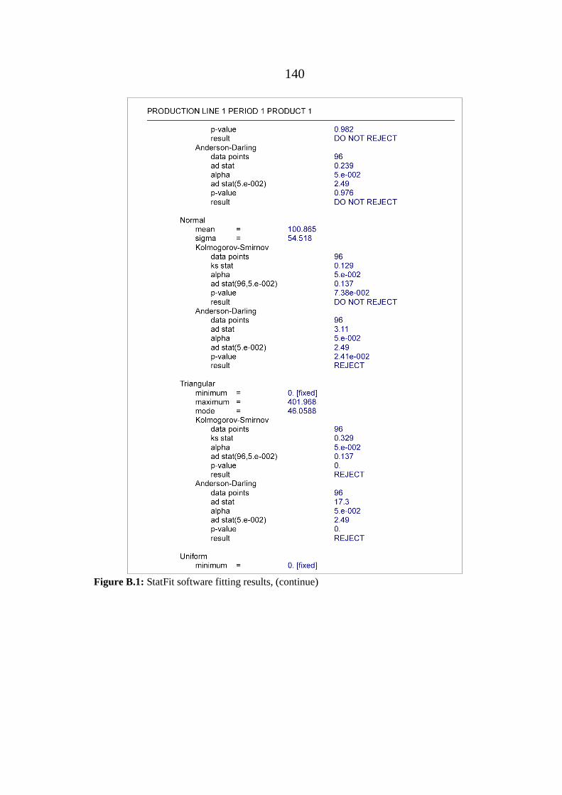
140

Figure B.1: StatFit software fitting results, (continue)

141

Figure B.1: StatFit software fitting results2-Product 6 daily demand ( month 1)

Figure B.2: Daily demand StatFit software fitting results, (continue)

142

Figure B.3: Daily demand StatFit software fitting results, (continue)

143

Figure B.3: Daily demand StatFit software fitting results

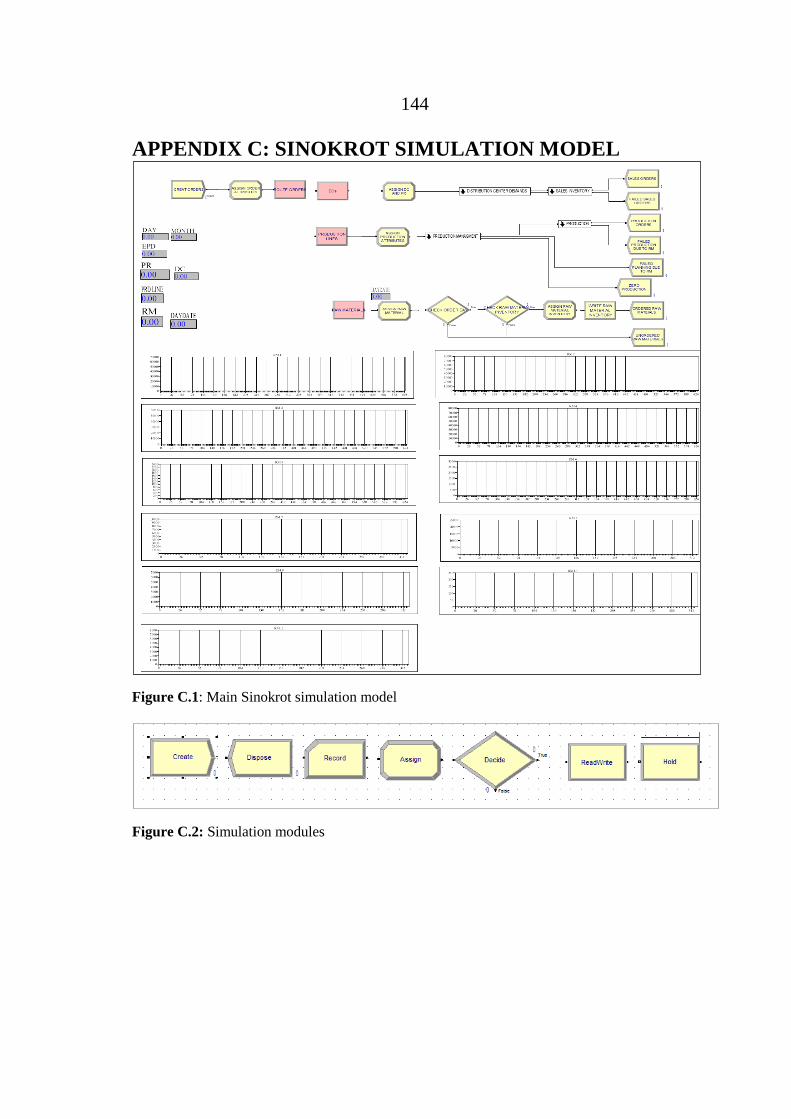
144

APPENDIX C: SINOKROT SIMULATION MODEL

Figure C.1: Main Sinokrot simulation model

Figure C.2: Simulation modules

145

Figure C.3: Structure of main Sinokrot simulation model (please see figures denoted by Cs for more detailes)

Figure C.4: Distribution centers demand and sales inventory

C.4

C.7

C.13

C.5 C.6

C.8

C.10

146

Figure C.5: Distribution centers demand sub-model

Figure C.6: Sales inventory sub-model

147

Figure C.7: Production mangment and production

Figure C.8: Production mangment sub-model

C.9

C.8 C.10

148

Figure C.9: Raw material requierment planning sub-model

Figure C.10: Production sub-model

C.11

1

C.12

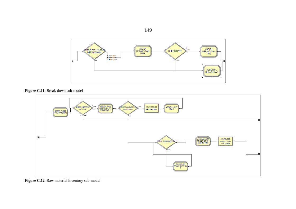
149

Figure C.11: Break-down sub-model

Figure C.12: Raw material inventory sub-model

150

Figure C.13: Raw material orders

151

Figure C.14: Structure of Sinokrot sales delivery simulation model (please see figures denoted by Cs for more detailes)

C.16

C.15

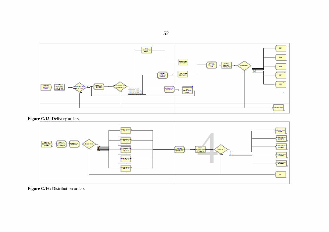
152

Figure C.15: Delivery orders

Figure C.16: Distribution orders

153

APPENDIX D: SIMULATION MODEL VALIDATION

1-DEMAND VALIDATION

Table (D.1): Real demand (semi-month demand of some products)

Product 1 Product 5 Product 10 Product 15 Product 17

Normal Normal Normal Normal Normal Normal

mean 57074.7 3185 399.042 2081.54 686.708

sigma 8405.59 849.428 287.709 795.315 526.072

Chi Squared

total classes 4 4 4 4 4

interval type equal probable equal probable equal probable equal probable equal probable

net bins 4 4 4 4 4

chi**2 1.33 1.33 1.67 2.33 8

degrees of

freedom 3 3 3 3 3

alpha 5.00E-02 5.00E-02 5.00E-02 5.00E-02 5.00E-02

chi**2(3,5.e-

002) 7.81 7.81 7.81 7.81 7.81

p-value 0.721 0.721 0.664 0.506 4.60E-02

result DO NOT

REJECT

DO NOT

REJECT

DO NOT

REJECT

DO NOT

REJECT REJECT

Kolmogorov-Smirnov

data points 24 24 24 24 24

ks stat 0.158 0.118 0.214 0.135 0.261

alpha 5.00E-02 5.00E-02 5.00E-02 5.00E-02 5.00E-02

ks stat(n,5.e-

002) 0.269 0.269 0.269 0.269 0.269

p-value 0.539 0.852 0.19 0.725 6.23E-02

result DO NOT

REJECT

DO NOT

REJECT

DO NOT

REJECT

DO NOT

REJECT

DO NOT

REJECT

Anderson-Darling

data points 24 24 24 24 24

ad stat 0.599 0.353 1.73 0.564 1.49

alpha 5.00E-02 5.00E-02 5.00E-02 5.00E-02 5.00E-02

ad stat(n,5.e-

002) 2.49 2.49 2.49 2.49 2.49

p-value 0.649 0.894 0.13 0.683 0.178

result DO NOT

REJECT

DO NOT

REJECT

DO NOT

REJECT

DO NOT

REJECT

DO NOT

REJECT

154

Table (D.2): Simulation model demand (semi-month demand of some

products)

Product 1 Product 5 Product 10 Product 15 Product 17

Normal Normal Normal Normal Normal Normal

mean 58220.4 3635.25 414.792 2125.92 707.958

sigma 6948.88 1498.24 292.944 788.259 531.319

Chi Squared

total classes 4 4 4 4 4

interval type equal probable equal probable equal probable equal probable equal probable

net bins 4 4 4 4 4

chi**2 6.67 5.33 4 4 8

degrees of

freedom 3 3 3 3 3

alpha 5.00E-02 5.00E-02 5.00E-02 5.00E-02 5.00E-02

chi**2(3,5.e-

002) 7.81 7.81 7.81 7.81 7.81

p-value 8.33E-02 0.149 0.261 0.261 4.60E-02

result DO NOT

REJECT

DO NOT

REJECT

DO NOT

REJECT

DO NOT

REJECT REJECT1

Kolmogorov-Smirnov

data points 24 24 24 24 24

ks stat 0.236 0.218 0.209 0.165 0.239

alpha 5.00E-02 5.00E-02 5.00E-02 5.00E-02 5.00E-02

ks stat(n,5.e-

002) 0.269 0.269 0.269 0.269 0.269

p-value 0.117 0.176 0.215 0.484 0.108

result DO NOT

REJECT

DO NOT

REJECT

DO NOT

REJECT

DO NOT

REJECT

DO NOT

REJECT

Anderson-Darling

data points 24 24 24 24 24

ad stat 1.19 1.44 1.71 0.714 1.57

alpha 5.00E-02 5.00E-02 5.00E-02 5.00E-02 5.00E-02

ad stat(n,5.e-

002) 2.49 2.49 2.49 2.49 2.49

p-value 0.27 0.192 0.134 0.548 0.161

result DO NOT

REJECT

DO NOT

REJECT

DO NOT

REJECT

DO NOT

REJECT

DO NOT

REJECT

155

Table (D.3): Paired T-Test (Demand)

Paired Samples Statistics

Pair Mean N Std. Deviation Std. Error Mean

1 rdemand1 58220.3750 24 7098.33899 1448.94238

mdemand1 58225.1667 24 7135.35179 1456.49758

2 rdemand5 3185.0000 24 867.69780 177.11807

mdemand5 3635.2500 24 1530.46870 312.40562

3 rdemand10 399.0417 24 293.89698 59.99147

mdemand10 414.7917 24 299.24499 61.08313

4 rdemand15 3603.3750 24 5269.67894 1075.66871

mdenand15 3679.0833 24 5298.66993 1081.58647

Paired Samples Correlations

Pairs N Correlation Sig.

1 rdemand1 & mdemand1 24 .691 .000

2 rdemand5 & mdemand5 24 .473 .020

3 rdemand10 & mdemand10 24 .991 .000

4 rdemand15 & mdenand15 24 .987 .000

Paired Samples Test

Pairs Paired Differences t df Sig.

(2-

tailed

)

Mean Std.

Deviation

Std. Error

Mean

95% Confidence Interval

of the Difference

Lower Upper

1 rdemand1 -

mdemand1 -4.791 5592.451 1141.554 -2366.276 2356.693 -.004 23 .997

ye

s

2 rdemand5 -

mdemand5

-

450.250 1356.238 276.84 -1022.939 122.439 -1.62 23 .117

ye

s

3 rdemand10 -

mdemand10 -15.750 41.095 8.3885 -33.1029 1.602 -1.88 23 .073

ye

s

4 rdemand15 -

mdenand15 -75.708 864.740 176.514 -440.856 289.439 -.429 23 .672

ye

s

Rdemand i: real product i demand, mdemand i: simulation model product i demand

Table (D.4):Non-parametric test (rank sum test) (Demand)

Pairs U mean variance Z Z(CI=5%) H0:data groups

are similar

5 rdemand17 -

mdemand17

281 288 2352 -1.44 1.96 yes

156

Table (D.5): Demand validation summery

Pairs

Normal

(chi-

squired

test)

Non-

paramet

ric test

(rank

sum

test)

Natural

pairing

(paired T

test)

Varianc

es are

equal

(F test)

independency

(Independent

T test)

Smith-

Satterwaith

test

validation

1 rdemand1 &

mdemand1 yes ---- yes ------ ----- ----- yes

2 rdemand5 &


3 rdemand10 &


4 rdemand15 &

mdenand15 yes ---- yes ------ ----- ----- yes

5 rdemand17 &

mdemand17 no yes ---- ------ ----- ---- yes

Demand validation: yes

157

2-PRODUCTION RATE VALIDATION

Table (D.6): Real Production rate (production rate of some

products)(continue)

product Product 1 Product 5

period Period 1 Period 2 Period 1 Period 2

Normal Normal Normal Normal Normal

mean 5.12605 4.34918 51.5613 41.9132

sigma 1.28914 0.668508 19.6416 16.9344

Chi Squared

total classes 8 6 4 6

interval type equal probable equal probable equal probable equal probable

net bins 8 6 4 4

chi**2 21.7 7.24 0.478 9.2

degrees of freedom 7 5 3 3

alpha 5.00E-02 5.00E-02 5.00E-02 5.00E-02

chi**2(3,5.e-002) 14.1 11.1 7.81 7.81

p-value 2.84E-03 0.203 0.924

2.67E-02

result REJECT DO NOT

REJECT

DO NOT

REJECT

REJECT

Kolmogorov-Smirnov

data points 67 67 23 20

ks stat 0.167 0.113 9.40E-02 0.279

alpha 5.00E-02 5.00E-02 5.00E-02 5.00E-02

ks stat(n,5.e-002) 0.163 0.163 0.275 0.294

p-value 4.24E-02 0.333 0.975 7.20E-02


REJECT

DO NOT

REJECT

DO NOT

REJECT

Anderson-Darling


ad stat 3.48 1.28 0.222 2.47

alpha 5.00E-02 5.00E-02 5.00E-02 5.00E-02

ad stat(n,5.e-002) 2.49 2.49 2.49 2.49

p-value 1.56E-02 0.241 0.983 5.15E-02


REJECT

DO NOT

REJECT

DO NOT

REJECT

158

Table (D.6): Real Production rate (production rate of some products)




mean 88.0153 74.3043 24.5605 24.4694

sigma 21.0665 12.3169 6.91202 6.82463

Chi Squared



net bins 5 4 4 4

chi**2 14.6 15.4 2.33 1


alpha 5.00E-02 5.00E-02 5.00E-02 5.00E-02

chi**2(3,5.e-002) 9.49 7.81 7.81 7.81

p-value 5.70E-03 1.48E-03 0.506 0.801

result REJECT REJECT DO NOT

REJECT

DO NOT

REJECT

Kolmogorov-Smirnov


ks stat 0.213 0.203 0.171 0.145

alpha 5.00E-02 5.00E-02 5.00E-02 5.00E-02

ks stat(n,5.e-002) 0.234 0.25 0.269 0.269

p-value 9.30E-02 0.172 0.434 0.643

result DO NOT

REJECT

DO NOT

REJECT

DO NOT

REJECT

DO NOT

REJECT

Anderson-Darling


ad stat 2.45 1.39 0.918 0.772

alpha 5.00E-02 5.00E-02 5.00E-02 5.00E-02

ad stat(n,5.e-002) 2.49 2.49 2.49 2.49

p-value 5.26E-02 0.204 0.403 0.502

result DO NOT

REJECT

DO NOT

REJECT

DO NOT

REJECT

DO NOT

REJECT

159

Table (D.6): Simulation Production rate (production rate of some

products) (continue)




mean 4.36555 4.15791 46.7296 50.9529

sigma 0.510217 0.649912 17.9501 4.007

Chi Squared



net bins 6 6 4 4

chi**2 2.04 0.791 6.74 1.2


alpha 5.00E-02 5.00E-02 5.00E-02 5.00E-02

chi**2(3,5.e-002) 11.1 11.1 7.81 7.81

p-value 0.843 0.978 8.07E-02 0.753

result DO NOT

REJECT

DO NOT

REJECT

DO NOT

REJECT

DO NOT

REJECT

Kolmogorov-Smirnov


ks stat 7.36E-02 6.26E-02 0.229 0.127

alpha 5.00E-02 5.00E-02 5.00E-02 5.00E-02

ks stat(n,5.e-002) 0.163 0.163 0.275 0.294

p-value 0.835 0.941 0.153 0.863

result DO NOT

REJECT

DO NOT

REJECT

DO NOT

REJECT

DO NOT

REJECT

Anderson-Darling


ad stat 0.441 0.259 1.3 0.344

alpha 5.00E-02 5.00E-02 5.00E-02 5.00E-02

ad stat(n,5.e-002) 2.49 2.49 2.49 2.49

p-value 0.808 0.965 0.232 0.901

result DO NOT

REJECT

DO NOT

REJECT

DO NOT

REJECT

DO NOT

REJECT

160

Table (D.6): Simulation Production rate (production rate of some

products)




mean 61.1722 59.2359 21.0882 27.3221

sigma 7.91833 7.43414 7.44759 6.8505

Chi Squared



net bins 4 4 4 5

chi**2 3.75 1.43 1.67 7.63


alpha 5.00E-02 5.00E-02 5.00E-02 5.00E-02

chi**2(3,5.e-002) 7.81 7.81 7.81 9.49

p-value 0.29 0.699 0.644 0.106

result DO NOT

REJECT

DO NOT

REJECT

DO NOT

REJECT

DO NOT

REJECT

Kolmogorov-Smirnov


ks stat 9.93E-02 0.103 0.132 0.121

alpha 5.00E-02 5.00E-02 5.00E-02 5.00E-02

ks stat(n,5.e-002) 0.234 0.25 0.269 0.192

p-value 0.88 0.9 0.747 0.452

result DO NOT

REJECT

DO NOT

REJECT

DO NOT

REJECT

DO NOT

REJECT

Anderson-Darling


ad stat 0.421 0.281 0.471 0.721

alpha 5.00E-02 5.00E-02 5.00E-02 5.00E-02

ad stat(n,5.e-002) 2.49 2.49 2.49 2.49

p-value 0.828 0.952 0.777 0.542

result DO NOT

REJECT

DO NOT

REJECT

DO NOT

REJECT

DO NOT

REJECT

161

Table (D.7): Paired T-Test (Production rate)


pairs Mean N Std. Deviation Std. Error Mean

2 rprivity1p2 4.3492 67 .67355 .08229

sprivity1p2 4.1579 67 .65482 .08000

3 rprivity5p1 51.5613 23 20.08308 4.18761

sprivity5p1 46.7296 23 18.35351 3.82697

7 rprivity17p1 24.5605 24 7.06068 1.44125

sprivity17p1 21.0882 24 7.60777 1.55293

8 rprivity17p2 27.5929 24 6.79021 1.38604

sprivity17p2 29.8716 24 7.30181 1.49047


pairs N Correlation Sig.

2 rprivity1p2 & sprivity1p2 67 .199 .107




Paired Samples Test

Pairs Paired Differences t df Sig.

(2-

tailed

)

Paired?

Mean Std.

Deviation

Std.

Error

Mean

95% Confidence

Interval of the

Difference

Lower Upper

2 rprivity1p2 - sprivity1p2 .191 .840 .102 -.0138 .396 1.862 66 .067 yes

3 rprivity5p1 - sprivity5p1 4.831 22.629 4.718 -4.954 14.617 1.024 22 .317 yes

7 rprivity17p1 - sprivity17p1 3.472 10.293 2.101 -.874 7.818 1.653 23 .112 yes

8 rprivity17p2 - sprivity17p2 -2.27 6.383 1.302 -4.973 .41665 -1.74 23 .094 yes

162

Table (D.8): Nonparametric test

pairs Hypothesis test summery

1 rprivity1p1 -

sprivity1p1

4 rprivity5p2 -

sprivity5p2

5 rprivity15p1-

sprivity15p1

6 rprivity15p2 -

sprivity15p2

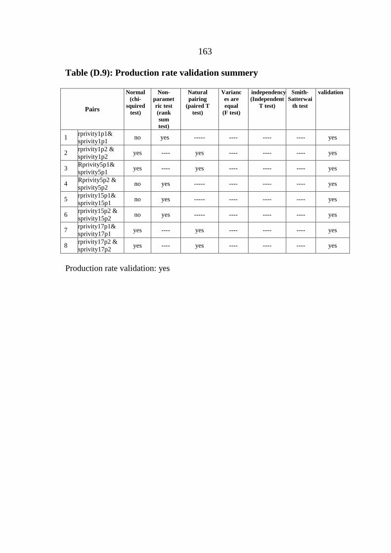
163

Table (D.9): Production rate validation summery

Pairs

Normal

(chi-

squired

test)

Non-

paramet

ric test

(rank

sum

test)

Natural

pairing

(paired T

test)

Varianc

es are

equal

(F test)

independency

(Independent

T test)

Smith-

Satterwai

th test

validation

1 rprivity1p1&

sprivity1p1 no yes ----- ---- ---- ---- yes

2 rprivity1p2 &

sprivity1p2 yes ---- yes ---- ---- ---- yes

3 Rprivity5p1&


4 Rprivity5p2 &


5 rprivity15p1&


6 rprivity15p2 &


7 rprivity17p1&


8 rprivity17p2 &


Production rate validation: yes

164

3. PRODUCED QUANTITIES VALIDATION

Table (D.10): Real produced quantities of some products

product Product 1 Product 5 Product 15 Product 17



mean 6183.1 311.9 484.906 1598.25

sigma 1702.36 96.9989 144.476 641.843

Chi Squared



net bins 6 4 4 4

chi**2 6.48 0.8 2.5 9.33


alpha 5.00E-02 5.00E-02 5.00E-02 5.00E-02

chi**2(3,5.e-002) 11.1 7.81 7.81 7.81

p-value 0.262 0.849 0.475 2.52E-02

result DO NOT

REJECT

DO NOT

REJECT

DO NOT

REJECT REJECT

Kolmogorov-Smirnov


ks stat 0.106 0.209 0.133 0.201

alpha 5.00E-02 5.00E-02 5.00E-02 5.00E-02

ks stat(n,5.e-002) 0.149 0.294 0.234 0.269

p-value 0.306 0.305 0.582 0.25

result DO NOT

REJECT

DO NOT

REJECT

DO NOT

REJECT

DO NOT

REJECT

Anderson-Darling


ad stat 1.39 0.967 0.43 1.31

alpha 5.00E-02 5.00E-02 5.00E-02 5.00E-02

ad stat(n,5.e-002) 2.49 2.49 2.49 2.49

p-value 0.206 0.375 0.818 0.23

result DO NOT

REJECT

DO NOT

REJECT

DO NOT

REJECT

DO NOT

REJECT

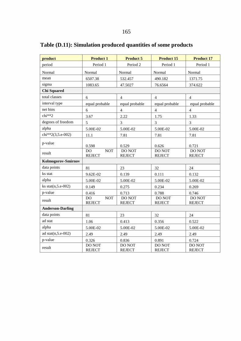
165

Table (D.11): Simulation produced quantities of some products

product Product 1 Product 5 Product 15 Product 17



mean 6507.38 532.457 490.182 1371.75

sigma 1083.65 47.5027 76.6564 374.622

Chi Squared



net bins 6 4 4 4

chi**2 3.67 2.22 1.75 1.33


alpha 5.00E-02 5.00E-02 5.00E-02 5.00E-02

chi**2(3,5.e-002) 11.1 7.81 7.81 7.81

p-value 0.598 0.529 0.626 0.721

result DO NOT

REJECT

DO NOT

REJECT

DO NOT

REJECT

DO NOT

REJECT

Kolmogorov-Smirnov


ks stat 9.62E-02 0.139 0.111 0.132

alpha 5.00E-02 5.00E-02 5.00E-02 5.00E-02

ks stat(n,5.e-002) 0.149 0.275 0.234 0.269

p-value 0.416 0.713 0.788 0.746

result DO NOT

REJECT

DO NOT

REJECT

DO NOT

REJECT

DO NOT

REJECT

Anderson-Darling


ad stat 1.06 0.413 0.356 0.522

alpha 5.00E-02 5.00E-02 5.00E-02 5.00E-02

ad stat(n,5.e-002) 2.49 2.49 2.49 2.49

p-value 0.326 0.836 0.891 0.724

result DO NOT

REJECT

DO NOT

REJECT

DO NOT

REJECT

DO NOT

REJECT

166

Table (D.12): Paired T-Test (produced quantities of some products)


pairs Mean N Std. Deviation Std. Error Mean

Pair 1

rprod1p1 6183.0988 81 1712.97168 190.33019

sprod1p1 6507.3751 81 1090.39949 121.15550

Pair 2

rprod5p2 311.9000 20 99.51879 22.25308

sprod5p2 369.2205 20 126.85253 28.36509

Pair 3

rprod15p1 484.9063 32 146.78739 25.94859

sprod15p1 490.1816 32 77.88298 13.76790


N Correlation Sig.

Pair 1 rprod1p1 & sprod1p1 81 .011 .925

Pair 2 rprod5p2 & sprod5p2 20 -.324- .163

Pair 3 rprod15p1 & sprod15p1 32 .483 .005

Paired Samples Test

Pairs Paired Differences t df Sig. (2-

tailed) Mean Std.

Deviation

Std. Error

Mean

95% Confidence

Interval of the

Difference

Lower Upper

1 rprod1p1 -

sprod1p1 -324.27 2020.79 224.532 -771.11 122.55 -1.44 80 .153

2 rprod5p2 -

sprod5p2 -57.32 184.89 41.344 -143.85 29.214 -1.38 19 .182

3 rprod15p1 -

sprod15p1 -5.27- 128.68 22.748 -51.67 41.120 -.23 31 .818

Table (D.13): Nonparametric test

pairs

1 rprod1p1 -

sprod1p1

167

Table (D.14): Demand validation summery

Pairs

Normal

(chi-

squired

test)

Non-

parametric

test

(rank

sum test)

Natural

pairing

(paired T

test)

Variances

are equal

(F test)

independency

(Independent T

test)

Smith-

Satterwaith

test

validation

1 rprod1p1 -

sprod1p1

yes ---- yes ------ ----- ----- yes

2 rprod5p2 -

sprod5p2

yes ---- yes ------ ----- ----- yes

3 rprod15p1 -

sprod15p1

yes ---- yes ------ ----- ----- yes

4 rprod17p1 -

sprod17p1

no yes ------ ------ ----- ----- yes

Produced Quantities Validation: yes

168

APPENDIX E: SIMULATIOM SCENARIOS

1-SCENARIO 1: MARKET DEMAND INCREASING (15%)

Table (E.1): Sales T-test and F-test results (scenario 1)(continue)

Group Statistics

Groups N Mean Std. Deviation Std. Error Mean

SP1 1.00 1103 1266.4757 1359.26595 40.92764

2.00 1018 3155.0027 50315.47104 1576.98533

SP6 1.00 102 146.3936 175.60210 17.38720

2.00 848 508.9612 7514.11555 258.03579

SP16 1.00 1199 7.3141 7.34402 .21209

2.00 1199 8.4111 8.41352 .24298

SP20 1.00 898 10.3280 8.88841 .29661

2.00 1041 21.0145 338.83335 10.50173

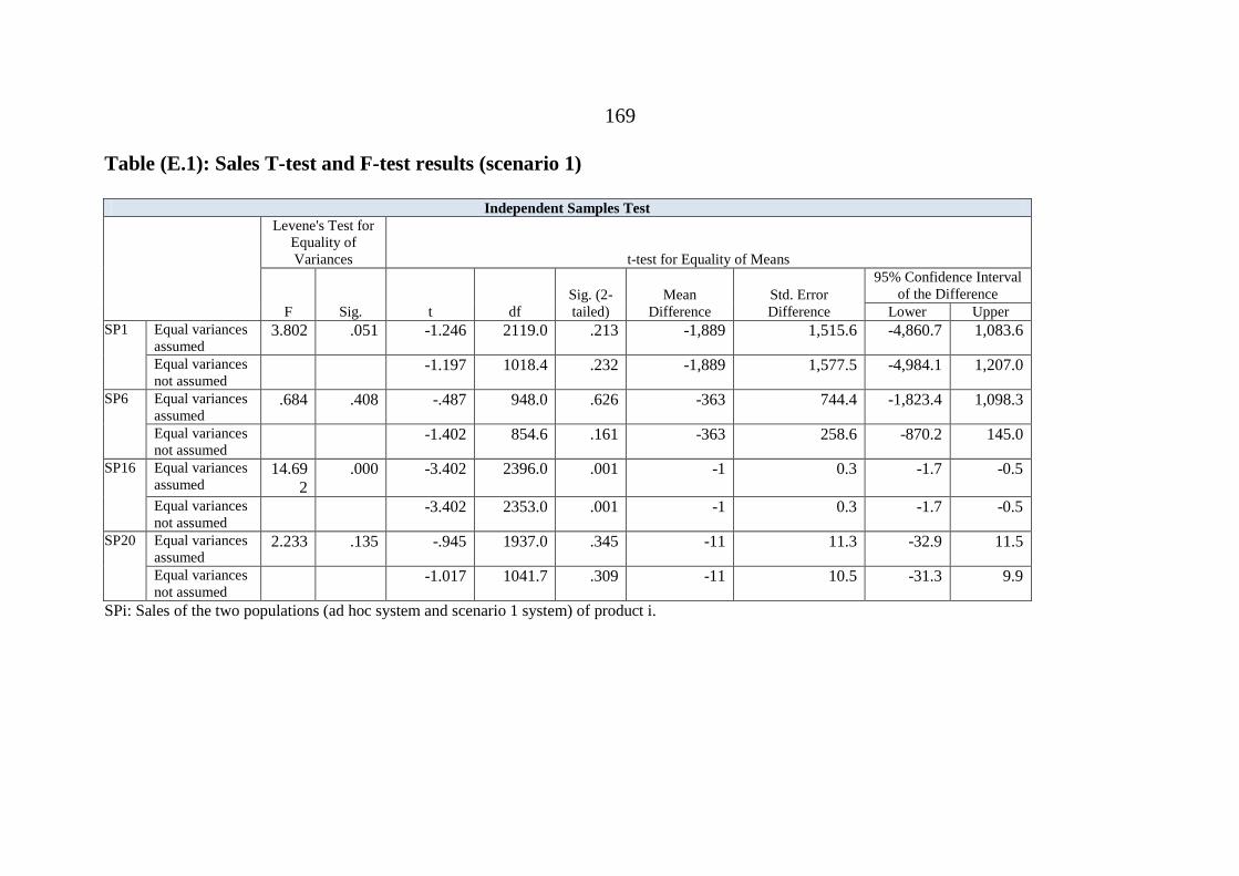
169

Table (E.1): Sales T-test and F-test results (scenario 1)

Independent Samples Test

Levene's Test for

Equality of

Variances t-test for Equality of Means

F Sig. t df

Sig. (2-

tailed)

Mean

Difference

Std. Error

Difference

95% Confidence Interval

of the Difference

Lower Upper

SP1 Equal variances

assumed 3.802 .051 -1.246 2119.0 .213 -1,889 1,515.6 -4,860.7 1,083.6

Equal variances

not assumed -1.197 1018.4 .232 -1,889 1,577.5 -4,984.1 1,207.0

SP6 Equal variances

assumed .684 .408 -.487 948.0 .626 -363 744.4 -1,823.4 1,098.3

Equal variances

not assumed -1.402 854.6 .161 -363 258.6 -870.2 145.0

SP16 Equal variances

assumed 14.69

2

.000 -3.402 2396.0 .001 -1 0.3 -1.7 -0.5

Equal variances

not assumed -3.402 2353.0 .001 -1 0.3 -1.7 -0.5

SP20 Equal variances

assumed 2.233 .135 -.945 1937.0 .345 -11 11.3 -32.9 11.5

Equal variances

not assumed -1.017 1041.7 .309 -11 10.5 -31.3 9.9

SPi: Sales of the two populations (ad hoc system and scenario 1 system) of product i.

170

SCENARIO 4: OPTIMUM RE-0RDER POINT IN CASE OF STOCHASTIC DEMAND AND LEAD TIME

Figure E.1:Scenario 4:Q-based inventory in case of stochastic demand and stochastic lead time

171

Table (E.2): Fixed Q-based raw material inventory (scenario 4)(continue)

T

heo

reti

cal

Qo

pt

×

Reo

rder

po

int

×

Raw material

1 2 3 4 5 6 7 8 9 10 11

Sto

ck o

ut

per

cen

tag

e

0.5 0.5 39% 29% 17% 24% 30% 7% 8% 21% 2% 40% 11%

0.5 1 9% 3% 2% 2% 15% 1% 2% 3% 1% 22% 5%

0.5 1.5 9% 3% 2% 2% 15% 1% 2% 3% 1% 22% 5%

0.5 2 0% 0% 0% 0% 1% 0% 0% 0% 0% 15% 1%

0.5 2.5 0% 0% 0% 0% 0% 0% 0% 0% 0% 4% 0%

1 0.5 10% 5% 4% 6% 7% 2% 2% 3% 0% 27% 4%

1 1 1% 1% 0% 1% 6% 0% 0% 1% 0% 23% 2%

1 1.5 0% 0% 0% 0% 3% 0% 0% 0% 0% 11% 1%

1 2 0% 0% 0% 0% 1% 0% 0% 0% 0% 5% 1%

1 2.5 0% 0% 0% 0% 0% 0% 0% 0% 0% 2% 0%

To

tal

inv

ento

ry c

ost

0.5 0.5 2,666,898 2,111,065 862,941 3,142,135 60,880 305,491 404,389 3,240,018 266,358 19,198 531,059

0.5 1 2,670,326 2,043,542 864,909 3,145,796 55,422 291,120 382,285 3,241,586 233,269 15,448 531,313

0.5 1.5 2,674,088 2,116,636 866,541 3,148,625 55,549 291,306 382,698 3,242,881 233,334 15,448 531,561

0.5 2 2,760,879 2,124,266 910,946 3,266,473 55,620 291,858 406,176 3,246,902 233,545 17,426 532,174

0.5 2.5 3,015,068 2,354,960 1,003,873 3,507,454 61,477 322,485 431,683 3,581,641 234,230 19,559 609,792

1 0.5 2,747,292 2,115,305 865,622 3,254,416 66,519 320,355 405,174 3,242,789 266,752 19,197 531,512

1 1 2,751,971 1,977,545 867,505 3,041,469 55,508 291,490 360,797 2,920,268 200,548 15,399 531,802

1 1.5 2,603,570 2,120,234 869,143 3,044,471 55,652 291,684 361,168 3,245,515 200,625 15,491 532,136

1 2 2,768,275 2,128,539 874,892 3,270,805 55,721 292,277 407,036 3,249,605 200,823 19,452 532,887

1 2.5 2,802,801 2,292,522 969,040 3,516,189 56,083 322,934 410,145 3,585,698 201,607 19,646 610,252

Key 2,666,898 Rejected solution , stock out percentage ≠0 2,920,268 Optimum inventory cost

172

Table (E.2): Fixed Q-based raw material inventory (scenario 4)(continue)

Th

eore

tica

l

Qo

pt

×

Reo

rder

po

int

×

Raw material

1 2 3 4 5 6 7 8 9 10 11

Sto

ck o

ut

per

cen

tag

e

1 2 0% 0% 0% 0% 1% 0% 0% 0% 0% 5% 1%

1 2.5 0% 0% 0% 0% 0% 0% 0% 0% 0% 2% 0%

1.5 0.5 3% 2% 2% 2% 3% 1% 1% 2% 0% 11% 2%

1.5 1 1% 1% 0% 0% 1% 0% 0% 0% 0% 10% 1%

1.5 1.5 0% 0% 0% 0% 1% 0% 0% 0% 0% 10% 1%

1.5 2 0% 0% 0% 0% 0% 0% 0% 0% 0% 9% 0%

1.5 2.5 0% 0% 0% 0% 0% 0% 0% 0% 0% 9% 0%

2 0.5 1% 0% 0% 1% 1% 0% 0% 0% 0% 2% 1%

2 1 0% 0% 0% 0% 0% 0% 0% 0% 0% 2% 1%

2 1.5 0% 0% 0% 0% 0% 0% 0% 0% 0% 2% 0%

To

tal

inv

ento

ry c

ost

1 2 2,768,275 2,128,539 874,892 3,270,805 55,721 292,277 407,036 3,249,605 200,823 19,452 532,887

1 2.5 2,802,801 2,292,522 969,040 3,516,189 56,083 322,934 410,145 3,585,698 201,607 19,646 610,252

1.5 0.5 2,753,338 2,119,700 947,174 3,261,253 66,731 306,360 406,216 3,407,714 300,665 23,161 456,535

1.5 1 2,757,351 1,911,152 832,025 2,939,788 50,266 262,936 339,438 2,923,457 201,349 17,442 456,812

1.5 1.5 2,761,113 2,125,068 833,657 2,942,658 50,305 263,102 339,776 2,924,683 201,439 17,442 456,985

1.5 2 2,545,329 2,133,475 839,172 3,277,975 50,340 263,639 407,928 2,928,773 201,608 17,447 457,852

1.5 2.5 2,545,329 2,133,475 839,172 3,277,975 50,340 263,639 407,928 2,928,773 201,608 17,447 457,852

2 0.5 2,771,853 2,135,710 959,747 3,279,322 67,345 351,534 409,932 3,903,908 401,774 23,599 459,280

2 1 2,775,435 1,716,080 727,530 2,634,025 34,415 264,618 276,009 2,934,266 202,944 12,171 459,488

2 1.5 2,779,197 2,138,951 729,239 2,636,770 34,493 264,783 276,280 2,935,765 202,944 12,171 459,834

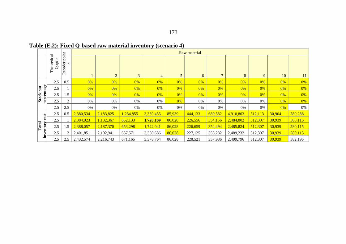
173

Table (E.2): Fixed Q-based raw material inventory (scenario 4)

T

heo

reti

cal

Qo

pt

×

Reo

rder

po

int

×

Raw material

1 2 3 4 5 6 7 8 9 10 11

Sto

ck o

ut

per

cen

tag

e 2.5 0.5 0% 0% 0% 0% 0% 0% 0% 0% 0% 0% 0%

2.5 1 0% 0% 0% 0% 0% 0% 0% 0% 0% 0% 0%

2.5 1.5 0% 0% 0% 0% 0% 0% 0% 0% 0% 0% 0%

2.5 2 0% 0% 0% 0% 0% 0% 0% 0% 0% 0% 0%

2.5 2.5 0% 0% 0% 0% 0% 0% 0% 0% 0% 0% 0%

To

tal

inv

ento

ry c

ost

2.5 0.5 2,380,534 2,183,825 1,234,855 3,339,455 85,939 444,133 689,582 4,910,803 512,113 30,904 580,288

2.5 1 2,384,923 1,132,367 652,133 1,720,169 86,028 226,556 354,156 2,484,802 512,307 30,939 580,115

2.5 1.5 2,388,057 2,187,370 653,298 1,722,041 86,028 226,659 354,494 2,485,824 512,307 30,939 580,115

2.5 2 2,401,851 2,192,941 657,571 3,350,686 86,028 227,125 355,282 2,489,232 512,307 30,939 580,115

2.5 2.5 2,432,574 2,216,743 671,165 3,378,764 86,028 228,521 357,986 2,499,796 512,307 30,939 582,195

174

Table (E.3): Raw material inventory level T-test and F-test results (ad hoc and scenario 4 models)

Group Statistics

RM N Mean

Std.

Deviation

Std. Error

Mean RM N Mean

Std.

Deviation

Std.

Error

Mean

RM

1 1.00 312 41,248 17,971 1,017

RM8 1.00 312 16,498 7,935 449

2.00 312 36,816 9,443 535 2.00 312 14,555 5,230 296

RM

4 1.00 312 47,359 22,551 1,277 RM1

1

1.00 312 4,378 1,890 107

2.00 312 24,786 7,187 407 2.00 312 2,677 866 49


Levene's Test for

Equality of


F Sig. t df

Sig.

(2-

tailed)

Mean

Difference

Std. Error

Difference

95% Confidence

Interval of the

Difference

Lower Upper

RM1 Equal variances assumed 108.7 .000 3.9 622.0 .000 4,432 1,149 2,175 6,689

Equal variances not assumed 3.9 470.6 .000 4,432 1,149 2,174 6,690



RM8 Equal variances assumed 56.9 .000 3.6 622.0 .000 1,943 538 886 2,999

Equal variances not assumed 3.6 538.3 .000 1,943 538 886 3,000

RM11 Equal variances assumed 149.6 .000 14.5 622.0 .000 1,702 118 1,471 1,933

Equal variances not assumed 14.5 436.1 .000 1,702 118 1,470 1,933

175

SCENARIO 5: OPTIMUM FIXED- TIME INVENTORY REVIEW IN CASE OF STOCHASTIC DEMAND AND

STOCHASTIC LEAD TIME

Figure E.2:Scenario 5:Inventory fixed-time revweing in case of stochastic demand and stochastic lead time

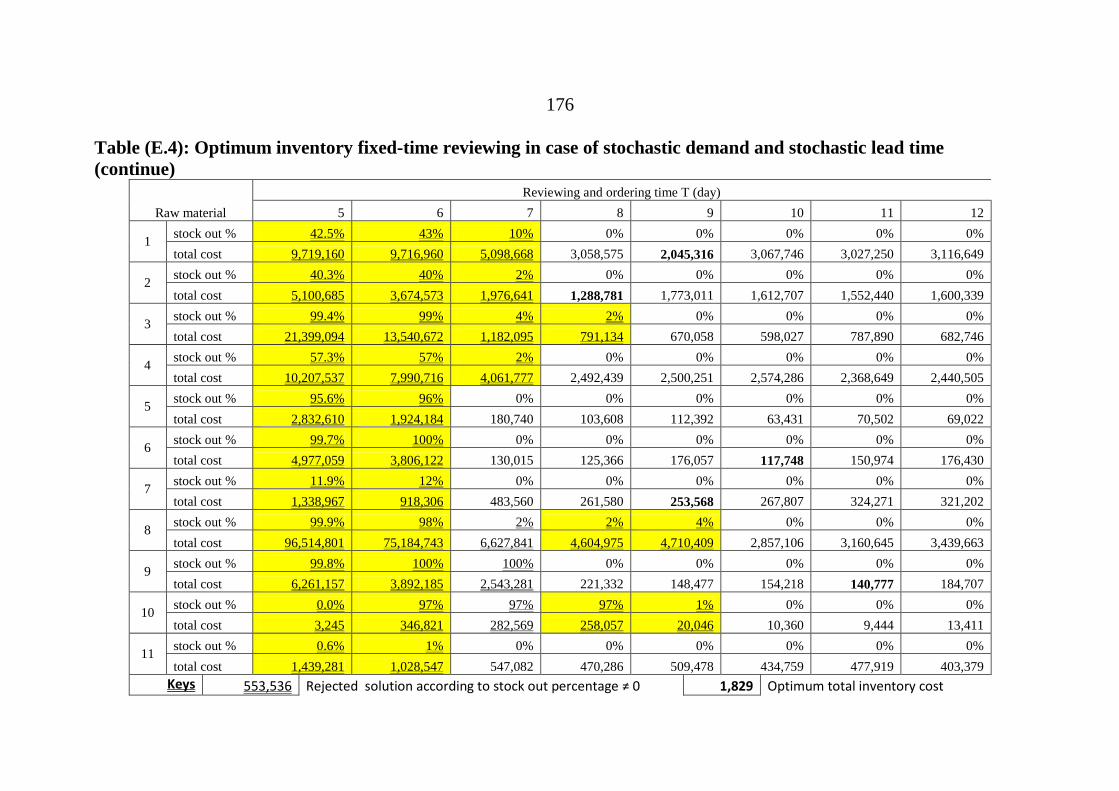
176

Table (E.4): Optimum inventory fixed-time reviewing in case of stochastic demand and stochastic lead time

(continue)

Raw material

Reviewing and ordering time T (day)

5 6 7 8 9 10 11 12

1 stock out % 42.5% 43% 10% 0% 0% 0% 0% 0%

total cost 9,719,160 9,716,960 5,098,668 3,058,575 2,045,316 3,067,746 3,027,250 3,116,649

2 stock out % 40.3% 40% 2% 0% 0% 0% 0% 0%

total cost 5,100,685 3,674,573 1,976,641 1,288,781 1,773,011 1,612,707 1,552,440 1,600,339

3 stock out % 99.4% 99% 4% 2% 0% 0% 0% 0%

total cost 21,399,094 13,540,672 1,182,095 791,134 670,058 598,027 787,890 682,746

4 stock out % 57.3% 57% 2% 0% 0% 0% 0% 0%

total cost 10,207,537 7,990,716 4,061,777 2,492,439 2,500,251 2,574,286 2,368,649 2,440,505

5 stock out % 95.6% 96% 0% 0% 0% 0% 0% 0%

total cost 2,832,610 1,924,184 180,740 103,608 112,392 63,431 70,502 69,022

6 stock out % 99.7% 100% 0% 0% 0% 0% 0% 0%

total cost 4,977,059 3,806,122 130,015 125,366 176,057 117,748 150,974 176,430

7 stock out % 11.9% 12% 0% 0% 0% 0% 0% 0%

total cost 1,338,967 918,306 483,560 261,580 253,568 267,807 324,271 321,202

8 stock out % 99.9% 98% 2% 2% 4% 0% 0% 0%

total cost 96,514,801 75,184,743 6,627,841 4,604,975 4,710,409 2,857,106 3,160,645 3,439,663

9 stock out % 99.8% 100% 100% 0% 0% 0% 0% 0%

total cost 6,261,157 3,892,185 2,543,281 221,332 148,477 154,218 140,777 184,707

10 stock out % 0.0% 97% 97% 97% 1% 0% 0% 0%

total cost 3,245 346,821 282,569 258,057 20,046 10,360 9,444 13,411

11 stock out % 0.6% 1% 0% 0% 0% 0% 0% 0%

total cost 1,439,281 1,028,547 547,082 470,286 509,478 434,759 477,919 403,379

Keys 553,536 Rejected solution according to stock out percentage ≠ 0 1,829 Optimum total inventory cost

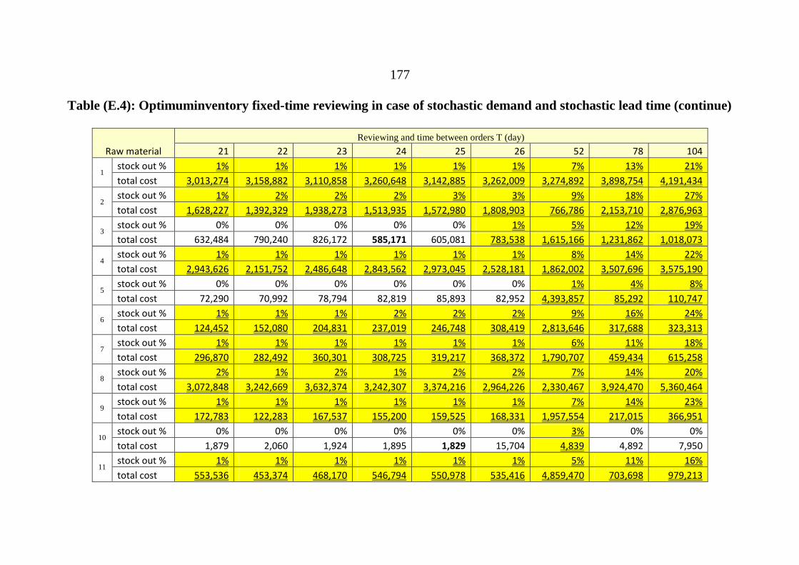
177

Table (E.4): Optimuminventory fixed-time reviewing in case of stochastic demand and stochastic lead time (continue)

Raw material

Reviewing and time between orders T (day)

21 22 23 24 25 26 52 78 104

1 stock out % 1% 1% 1% 1% 1% 1% 7% 13% 21%

total cost 3,013,274 3,158,882 3,110,858 3,260,648 3,142,885 3,262,009 3,274,892 3,898,754 4,191,434

2 stock out % 1% 2% 2% 2% 3% 3% 9% 18% 27%

total cost 1,628,227 1,392,329 1,938,273 1,513,935 1,572,980 1,808,903 766,786 2,153,710 2,876,963

3 stock out % 0% 0% 0% 0% 0% 1% 5% 12% 19%

total cost 632,484 790,240 826,172 585,171 605,081 783,538 1,615,166 1,231,862 1,018,073

4 stock out % 1% 1% 1% 1% 1% 1% 8% 14% 22%

total cost 2,943,626 2,151,752 2,486,648 2,843,562 2,973,045 2,528,181 1,862,002 3,507,696 3,575,190

5 stock out % 0% 0% 0% 0% 0% 0% 1% 4% 8%

total cost 72,290 70,992 78,794 82,819 85,893 82,952 4,393,857 85,292 110,747

6 stock out % 1% 1% 1% 2% 2% 2% 9% 16% 24%

total cost 124,452 152,080 204,831 237,019 246,748 308,419 2,813,646 317,688 323,313

7 stock out % 1% 1% 1% 1% 1% 1% 6% 11% 18%

total cost 296,870 282,492 360,301 308,725 319,217 368,372 1,790,707 459,434 615,258

8 stock out % 2% 1% 2% 1% 2% 2% 7% 14% 20%

total cost 3,072,848 3,242,669 3,632,374 3,242,307 3,374,216 2,964,226 2,330,467 3,924,470 5,360,464

9 stock out % 1% 1% 1% 1% 1% 1% 7% 14% 23%

total cost 172,783 122,283 167,537 155,200 159,525 168,331 1,957,554 217,015 366,951

10 stock out % 0% 0% 0% 0% 0% 0% 3% 0% 0%

total cost 1,879 2,060 1,924 1,895 1,829 15,704 4,839 4,892 7,950

11 stock out % 1% 1% 1% 1% 1% 1% 5% 11% 16%

total cost 553,536 453,374 468,170 546,794 550,978 535,416 4,859,470 703,698 979,213

178

Table (E.4): Optimuminventory fixed-time reviewing in case of stochastic demand and stochastic lead time (continue)

Raw material

Reviewing and time between orders T (day)

13 14 15 16 17 18 19 20

1 stock out % 0% 0% 0% 0% 0% 0% 0% 0%

total cost 3,128,874 3,095,813 3,022,980 3,047,155 3,100,135 3,122,897 3,104,562 3,082,277

2 stock out % 0% 1% 1% 1% 1% 1% 1% 1%

total cost 1,467,005 1,474,685 1,781,880 2,014,530 1,670,328 1,519,914 1,593,897 1,820,990

3 stock out % 0% 0% 0% 0% 0% 0% 0% 0%

total cost 620,551 706,983 673,083 626,558 611,052 753,253 742,210 833,377

4 stock out % 0% 0% 0% 0% 1% 1% 1% 1%

total cost 2,646,733 2,109,466 2,570,936 2,239,768 2,570,904 2,325,501 2,849,477 2,803,843

5 stock out % 0% 0% 0% 0% 0% 0% 0% 0%

total cost 67,847 67,408 66,659 69,858 64,522 72,938 62,017 68,425

6 stock out % 0% 0% 0% 0% 1% 1% 1% 1%

total cost 190,870 206,329 147,592 188,632 217,214 106,762 131,389 255,251

7 stock out % 0% 0% 0% 0% 0% 0% 1% 1%

total cost 311,736 336,146 338,149 406,161 312,903 356,345 270,123 311,610

8 stock out % 0% 0% 0% 1% 0% 1% 1% 1%

total cost 3,308,842 2,274,874 3,026,473 3,107,781 3,409,455 3,159,459 3,247,114 2,756,837

9 stock out % 0% 0% 0% 0% 0% 1% 1% 1%

total cost 165,580 153,722 189,918 161,901 156,483 133,001 174,873 163,274

10 stock out % 0% 1% 0% 0% 1% 0% 0% 1%

total cost 2,090 10,811 13,658 2,098 13,007 13,707 2,317 11,923

11 stock out % 0% 0% 0% 0% 0% 0% 0% 1%

total cost 541,220 393,307 508,206 512,488 446,001 543,336 503,350 601,206

179

Table (E.4): Optimum inventory fixed-time reviewing in case of stochastic demand and stochastic lead time

Raw 1 2 3 4 5 6

stock

out %

total cost stock

out %

total cost stock

out %

total cost stock

out %

total cost stock

out %

total cost stock

out %

total cost

T

5 42.5% 9,719,160 40.3% 5,100,685 99.4% 21,399,094 57.3% 10,207,537 95.6% 2,832,610 99.7% 4,977,059

6 43% 9,716,960 40% 3,674,573 99% 13,540,672 57% 7,990,716 96% 1,924,184 100% 3,806,122

7 10% 5,098,668 2% 1,976,641 4% 1,182,095 2% 4,061,777 0% 180,740 0% 130,015

8 0% 3,058,575 0% 1,288,781 2% 791,134 0% 2,492,439 0% 103,608 0% 125,366

9 0% 2,045,316 0% 1,773,011 0% 670,058 0% 2,500,251 0% 112,392 0% 176,057

10 0% 3,067,746 0% 1,612,707 0% 598,027 0% 2,574,286 0% 63,431 0% 117,748

11 0% 3,027,250 0% 1,552,440 0% 787,890 0% 2,368,649 0% 70,502 0% 150,974

12 0% 3,116,649 0% 1,600,339 0% 682,746 0% 2,440,505 0% 69,022 0% 176,430

13 0% 3,128,874 0% 1,467,005 0% 620,551 0% 2,646,733 0% 67,847 0% 190,870

14 0% 3,095,813 1% 1,474,685 0% 706,983 0% 2,109,466 0% 67,408 0% 206,329

15 0% 3,022,980 1% 1,781,880 0% 673,083 0% 2,570,936 0% 66,659 0% 147,592

16 0% 3,047,155 1% 2,014,530 0% 626,558 0% 2,239,768 0% 69,858 0% 188,632

17 0% 3,100,135 1% 1,670,328 0% 611,052 1% 2,570,904 0% 64,522 1% 217,214

18 0% 3,122,897 1% 1,519,914 0% 753,253 1% 2,325,501 0% 72,938 1% 106,762

19 0% 3,104,562 1% 1,593,897 0% 742,210 1% 2,849,477 0% 62,017 1% 131,389

20 0% 3,082,277 1% 1,820,990 0% 833,377 1% 2,803,843 0% 68,425 1% 255,251

21 1% 3,013,274 1% 1,628,227 0% 632,484 1% 2,943,626 0% 72,290 1% 124,452

22 1% 3,158,882 2% 1,392,329 0% 790,240 1% 2,151,752 0% 70,992 1% 152,080

23 1% 3,110,858 2% 1,938,273 0% 826,172 1% 2,486,648 0% 78,794 1% 204,831

24 1% 3,260,648 2% 1,513,935 0% 585,171 1% 2,843,562 0% 82,819 2% 237,019

25 1% 3,142,885 3% 1,572,980 0% 605,081 1% 2,973,045 0% 85,893 2% 246,748

26 1% 3,262,009 3% 1,808,903 1% 783,538 1% 2,528,181 0% 82,952 2% 308,419

52 7% 3,274,892 9% 766,786 5% 1,615,166 8% 1,862,002 1% 4,393,857 9% 2,813,646

78 13% 3,898,754 18% 2,153,710 12% 1,231,862 14% 3,507,696 4% 85,292 16% 317,688

104 21% 4,191,434 27% 2,876,963 19% 1,018,073 22% 3,575,190 8% 110,747 24% 323,313

180

Table (E.5): Scenario5: Raw material inventory level T-test and F-test results

Group Statistics

RM N Mean

Std.

Deviation

Std. Error

Mean RM N Mean

Std.

Deviation

Std.

Error

Mean

RM1 1.00 41,248 17,971 1,017 41,248 RM8

1.00 312 16,498 7,935 449

2.00 21,496 8,195 460 21,496 2.00 312 8,449 3,965 223

RM4 1.00 47,359 22,551 1,277 47,359 RM11

1.00 312 4,378 1,890 107

2.00 15,462 7,399 416 15,462 2.00 312 928 332 19


Levene's Test for

Equality of


F Sig. t df

Sig.

(2-

tailed)

Mean

Difference

Std. Error

Difference

95% Confidence

Interval of the

Difference

Lower Upper





RM8 Equal variances assumed 56.9 .000 3.6 622.0 .000 1,943 538 886 2,999

Equal variances not assumed 3.6 538.3 .000 1,943 538 886 3,000

RM11 Equal variances assumed 149.6 .000 14.5 622.0 .000 1,702 118 1,471 1,933

Equal variances not assumed 14.5 436.1 .000 1,702 118 1,470 1,933

ملخص ال

simulation modeling applications in organization management shweikeh_0.pdf · simulation modeling...

Documents