simulation of a slope stability radar for opencast...

Simulation of a Slope Stability Radarfor Opencast Mining

Daniel John Tanser

A dissertation submitted to the Department of Electrical Engineering,

University of Cape Town, in fulfillment of the requirements

for the degree of Master of Science in Engineering.

Cape Town, March 2003

Declaration

I declare that this dissertation is my own, unaided work. It is being submitted for the

degree of Master of Science in Engineering in the University of Cape Town. It has not

been submitted before for any degree or examination in any other university.

Signature of Author . . . . . . . . . . . . . . . . . . . . . . . . . . . . . . . . . . . . . . . . . . . . . . . . . . . . . . . . . . . . . .

Cape Town

10 March 2002

i

Abstract

The suitability of a radar as a slope stability monitor for an opencast mine is investigated.

The radar is required to detect the millimetric pre-cursory movements of a wall face which

signal instability. An application-specific simulation was written in Matlab in order to de-

velop a differential interferometric algorithm to detect any movement. This algorithm was

applied to real data and performed adequately. Temporal decorrelation and atmospheric

variations were identified as likely error sources, and were investigated in turn using the

simulation. Based on the results of the simulation, a scanning procedure is proposed to

minimise these potential error sources. The radar is assessed as a very suitable technique

for monitoring slope stability. It is very accurate as an indicator of zero movement, and

performs within the specified millimetric precision for small movements (less than 2 mm).

For larger movements, the radar indicates that a movement has occurred but the accuracy

is reduced. These larger movements are unlikely to occur with the proposed scanning

procedure.

ii

Acknowledgements

The author would like to thank the following for their assistance with this thesis:

• Professor Inggs for his advice and guidance throughout the thesis;

• Dr. Andrew Wilkinson for his technical insight;

• Dr. Richard Lord for his patient proof-reading and assistance with this document;

• My brother, Dr. Frank Tanser, for his valuable advice on writing up;

• My digs-mates and friends for their continual mockery of my extended academic

career;

• My family for their continued support and prayers;

• The Lord, in whose strength this was done.

iii

Contents

Declaration i

Abstract ii

Acknowledgements iii

1 Introduction 1

1.1 Background . . . . . . . . . . . . . . . . . . . . . . . . . . . . . . . . . 1

1.2 User Requirements . . . . . . . . . . . . . . . . . . . . . . . . . . . . . 1

1.3 Possible Methods . . . . . . . . . . . . . . . . . . . . . . . . . . . . . . 1

1.3.1 Seismic Monitoring . . . . . . . . . . . . . . . . . . . . . . . . . 2

1.3.2 Radar . . . . . . . . . . . . . . . . . . . . . . . . . . . . . . . . 2

1.3.3 Laser . . . . . . . . . . . . . . . . . . . . . . . . . . . . . . . . 2

1.3.4 Photogrammetry . . . . . . . . . . . . . . . . . . . . . . . . . . 3

1.4 Motivation for the Use of Radar . . . . . . . . . . . . . . . . . . . . . . 3

1.5 Previous Work in Slope Monitoring Using Radar . . . . . . . . . . . . . 3

1.6 Scope and Limitations . . . . . . . . . . . . . . . . . . . . . . . . . . . 4

1.7 Project Overview . . . . . . . . . . . . . . . . . . . . . . . . . . . . . . 4

2 Stepped Frequency Radar 6

2.1 Concept of Stepped Frequency Radar . . . . . . . . . . . . . . . . . . . 6

2.2 Parameters of the Radar . . . . . . . . . . . . . . . . . . . . . . . . . . . 6

2.3 Setup of the Radar . . . . . . . . . . . . . . . . . . . . . . . . . . . . . 7

2.4 Overview of Radar Interferometry . . . . . . . . . . . . . . . . . . . . . 8

3 Simulation of a Single Cell of a Scan 10

3.1 Concept of the Matlab Simulation . . . . . . . . . . . . . . . . . . . . . 10

iv

3.1.1 Generation of Points to Simulate a Plane Target . . . . . . . . . . 10

3.1.2 Calculation of the Summed Frequency Response . . . . . . . . . 12

3.1.3 Noise Modeling . . . . . . . . . . . . . . . . . . . . . . . . . . . 12

3.1.4 Modeling a Shift in Range . . . . . . . . . . . . . . . . . . . . . 12

3.2 Frequency Domain Processing Techniques . . . . . . . . . . . . . . . . . 13

3.2.1 Zero Padding to Increase Display Resolution . . . . . . . . . . . 13

3.2.2 Windowing to Reduce Sidelobe Levels . . . . . . . . . . . . . . 13

3.2.3 Base-Banding to Remove Phase Slope . . . . . . . . . . . . . . . 13

3.3 Determination of the Change in Range . . . . . . . . . . . . . . . . . . . 16

3.3.1 Transformation into the Time Domain . . . . . . . . . . . . . . . 16

3.3.2 Phase Correlation . . . . . . . . . . . . . . . . . . . . . . . . . . 16

3.3.3 Phase Difference . . . . . . . . . . . . . . . . . . . . . . . . . . 19

3.3.4 Ambiguity in Differential Phase . . . . . . . . . . . . . . . . . . 21

3.3.5 Identification of the Region of Interest . . . . . . . . . . . . . . . 21

3.3.6 Removal of2π Jumps in the Phase Values . . . . . . . . . . . . . 21

3.3.7 Computation of Shift in Range . . . . . . . . . . . . . . . . . . . 22

3.4 Results of the Simulation . . . . . . . . . . . . . . . . . . . . . . . . . . 23

3.5 Conclusion . . . . . . . . . . . . . . . . . . . . . . . . . . . . . . . . . 26

4 Experimental Readings of a Single Cell 27

4.1 Parameters of Radar Used for Readings . . . . . . . . . . . . . . . . . . 27

4.2 Modifications to the Algorithm . . . . . . . . . . . . . . . . . . . . . . . 29

4.2.1 Summation of Scans to Improve SNR . . . . . . . . . . . . . . . 30

4.2.2 Apparent Warping of Wall Due to High Beamwidth . . . . . . . . 30

4.2.3 Change in Bandwidth to Remove Errors in Gross Shift . . . . . . 33

4.3 Results of the Experimental Readings . . . . . . . . . . . . . . . . . . . 33

4.3.1 Fine Shift Errors . . . . . . . . . . . . . . . . . . . . . . . . . . 33

4.3.2 Gross Shift Errors . . . . . . . . . . . . . . . . . . . . . . . . . 33

4.4 Conclusion . . . . . . . . . . . . . . . . . . . . . . . . . . . . . . . . . 36

5 Simulation of an Entire Scan 37

5.1 Concept of the Matlab Simulation . . . . . . . . . . . . . . . . . . . . . 37

5.1.1 Generation of Points to Simulate a Wall Face . . . . . . . . . . . 37

v

5.1.2 Modeling a Shift in Range . . . . . . . . . . . . . . . . . . . . . 37

5.2 Results of the Extended Simulation - Mass Movement . . . . . . . . . . 39

5.2.1 Fine Shift Errors . . . . . . . . . . . . . . . . . . . . . . . . . . 41

5.2.2 Gross Shift Errors . . . . . . . . . . . . . . . . . . . . . . . . . 41

5.3 Conclusion . . . . . . . . . . . . . . . . . . . . . . . . . . . . . . . . . 42

6 Temporal Decorrelation 44

6.1 Definition of Temporal Decorrelation . . . . . . . . . . . . . . . . . . . 44

6.2 Confidence Value - the Peak of the Phase Correlation Curve . . . . . . . 45

6.3 Temporal Decorrelation Due to a Change in Angle . . . . . . . . . . . . 46

6.3.1 Modeling a Change in Angle . . . . . . . . . . . . . . . . . . . . 46

6.3.2 Decrease in Correlation Due to a Change in Angle . . . . . . . . 46

6.3.3 Results of the Simulation for a Change in Angle . . . . . . . . . 46

6.4 Temporal Decorrelation Due to a Localised Shift . . . . . . . . . . . . . 51

6.4.1 Modeling a Localised Shift . . . . . . . . . . . . . . . . . . . . . 51

6.4.2 Average Shift of the Entire Cell . . . . . . . . . . . . . . . . . . 51

6.4.3 Decrease in Correlation Due to a Localised Shift . . . . . . . . . 51

6.4.4 Results of the Simulation for a Localised Shift . . . . . . . . . . 51

6.5 Results of the Simulation For a Wedge Failure . . . . . . . . . . . . . . . 56

6.5.1 Modeling a Wedge Failure . . . . . . . . . . . . . . . . . . . . . 56

6.5.2 Results of the Simulation for a Wedge Failure . . . . . . . . . . . 56

6.6 Conclusion . . . . . . . . . . . . . . . . . . . . . . . . . . . . . . . . . 60

6.6.1 Summary of the Results of the Simulation . . . . . . . . . . . . . 60

6.6.2 Confidence Value as a Measure of Stability . . . . . . . . . . . . 60

6.6.3 Change in Procedure to Reduce Temporal Decorrelation . . . . . 61

7 Atmospheric Variations 62

7.1 Effect of Atmospheric Variations . . . . . . . . . . . . . . . . . . . . . . 62

7.2 Simulation of a Corner Reflector . . . . . . . . . . . . . . . . . . . . . . 63

7.3 Simulation of a Change in Atmospheric Conditions . . . . . . . . . . . . 63

7.3.1 Change in Temperature . . . . . . . . . . . . . . . . . . . . . . . 64

7.3.2 Change in Pressure . . . . . . . . . . . . . . . . . . . . . . . . . 66

7.3.3 Change in Partial Pressure of Water Vapour . . . . . . . . . . . . 66

vi

7.4 Variation of Atmospheric Effects With Range . . . . . . . . . . . . . . . 67

7.5 Updated Algorithm . . . . . . . . . . . . . . . . . . . . . . . . . . . . . 70

7.6 Results of the Simulation . . . . . . . . . . . . . . . . . . . . . . . . . . 71

7.7 Conclusion . . . . . . . . . . . . . . . . . . . . . . . . . . . . . . . . . 71

8 Conclusions 73

8.1 Review of the Thesis . . . . . . . . . . . . . . . . . . . . . . . . . . . . 73

8.2 Summary of the Results . . . . . . . . . . . . . . . . . . . . . . . . . . . 75

8.3 Final Assessment of Technique . . . . . . . . . . . . . . . . . . . . . . . 75

8.4 Recommended Scanning Procedure . . . . . . . . . . . . . . . . . . . . 76

A Simulation of a Single Cell of a Scan 83

B Processing of Real Data Using the Algorithm 88

C Expanded Simulation of an Entire Scan 92

vii

List of Figures

2.1 Approximate Layout of the Mine . . . . . . . . . . . . . . . . . . . . . . 9

3.1 Point Targets Generated to Simulate a Planar Target . . . . . . . . . . . . 11

3.2 Zero Padding the Frequency Response to Increase Display Resolution in

the Time Domain . . . . . . . . . . . . . . . . . . . . . . . . . . . . . . 14

3.3 Multiplication of the Frequency Response by a Hanning Window in order

to Decrease Sidelobe Levels in the Time Domain . . . . . . . . . . . . . 15

3.4 Base-banding the Frequency Response in order to Remove the Phase

Slope in the Time Domain . . . . . . . . . . . . . . . . . . . . . . . . . 17

3.5 Range Profiles of Two Scans with a Shift in Range of 1 mm . . . . . . . . 18

3.6 Phase Correlation of Two Scans with a Shift of 15 mm . . . . . . . . . . 20

3.7 Flow-chart of the Stepped Frequency Simulation . . . . . . . . . . . . . 24

3.8 Error in Shifts Calculated Using the Simulation . . . . . . . . . . . . . . 25

4.1 The Arrangement of the Radar used to Take Real Readings of a Shift in

Range of a Wall. The Approximate Footprint is Sketched on the Wall. . . 28

4.2 Range Profiles of Scans at 65 and 60 cm . . . . . . . . . . . . . . . . . . 29

4.3 Geometry of the Real Readings, Illustrating the Difference Betweenr1

andr2 . . . . . . . . . . . . . . . . . . . . . . . . . . . . . . . . . . . . 31

4.4 Decrease in Correlation Due to Apparent Warping as a Result of the High

Beamwidth . . . . . . . . . . . . . . . . . . . . . . . . . . . . . . . . . 32

4.5 Error in Shifts Calculated Using the Real Data . . . . . . . . . . . . . . . 35

5.1 Simulation of an Entire Scan . . . . . . . . . . . . . . . . . . . . . . . . 38

5.2 Mass Movement of Cells b2, b3 and b4 . . . . . . . . . . . . . . . . . . 39

5.3 Error in Shift Calculated Using the Simulation of an Entire Scan . . . . . 40

6.1 Variation of the Confidence Value with SNR for a Mass Movement of 1 mm 45

viii

6.2 Change in Angle of Cells b2, b3 and b4 . . . . . . . . . . . . . . . . . . 47

6.3 Decrease in Correlation Due to a Change in Angle . . . . . . . . . . . . . 48

6.4 Increase in the Magnitude of Fine Shift Errors for a Change in Angle as

the Confidence Value Decreases . . . . . . . . . . . . . . . . . . . . . . 49

6.5 Error in Shift in Range for a Change in Angle . . . . . . . . . . . . . . . 50

6.6 Localised Shift Resulting in a Change in Shape of Cell b3 . . . . . . . . . 52

6.7 Decrease in Correlation Due to a Localised Shift . . . . . . . . . . . . . 53

6.8 Increase in the Magnitude of Fine Shift Errors for a Localised Shift as the

Confidence Value Decreases . . . . . . . . . . . . . . . . . . . . . . . . 54

6.9 Error in Shift in Range for a Localised Shift . . . . . . . . . . . . . . . . 55

6.10 Modeling a Wedge Failure . . . . . . . . . . . . . . . . . . . . . . . . . 57

6.11 Increase in the Magnitude of Fine Shift Errors for a Wedge Failure as the

Confidence Value Decreases . . . . . . . . . . . . . . . . . . . . . . . . 58

6.12 Error in Shift in Range for Each Cell of a Simulated Wedge Failure . . . . 59

7.1 Range Profiles of the Reference Reflector . . . . . . . . . . . . . . . . . 63

7.2 Apparent Shift in Range Due to Changes in Temperature . . . . . . . . . 65

7.3 Apparent Shift in Range Due to Changes in Pressure . . . . . . . . . . . 66

7.4 The Partial Pressure of Water Vapour Modeled Using Relative Humidity . 68

7.5 Apparent Shift in Range Due to Variations in the Partial Pressure of Water 69

ix

List of Tables

3.1 Selected Results for the Error in Shift in Range Obtained Using the Sim-

ulation . . . . . . . . . . . . . . . . . . . . . . . . . . . . . . . . . . . . 23

4.1 Average Shift Across the Entire Scan for Various Readings . . . . . . . . 31

4.2 Error in Shift in Range Using the Real Data . . . . . . . . . . . . . . . . 34

5.1 Accuracy of the Fine Shift Calculation of Shift in Range . . . . . . . . . 41

7.1 The Variation of Atmospheric Effect With Range . . . . . . . . . . . . . 70

7.2 Change in Atmospheric Conditions Between the Two Scans . . . . . . . . 71

7.3 Errors in Cells b2, b3 and b4 for Random Atmospheric Variations . . . . 72

x

Chapter 1

Introduction

1.1 Background

A method is required to monitor the stability of the wall of an opencast diamond mine in

Limpopo Province, South Africa. A collapse is signaled by small pre-cursory movements

as the wall de-stabilises. These small movements can be detected to identify unstable

regions and steps can be taken to avoid catastrophic collapse. It has been proposed that

a slope stability monitor be developed to scan the wall of the mine on a daily basis and

detect these pre-cursory movements.

1.2 User Requirements

The following requirements were specified for the slope stability monitor:

• The pre-cursory movements are very small, so the method will be required to detect

millimetric movements over a relatively large range (up to about 300m);

• Low cost i.e. low system complexity;

• Non-contact, so no hardware such as reflectors or sensors need be placed on the

wall of the mine;

• Robust, to endure the conditions at the mine.

1.3 Possible Methods

A number of methods to monitor ground stability exist. Only methods which monitor

the entire surface of the mine are discussed here. Some point displacement monitor-

1

ing techniques, used to monitor specific portions of the mine which have been identified

as unstable, such as inclinometers and time domain reflectometry, are described in [1]

and [2].

1.3.1 Seismic Monitoring

Routine seismic monitoring has been in use in gold mines for over 30 years in South

Africa [3]. The magnitude of seismic events triggered by blasting is measured at selected

locations throughout the mine in order to identify unstable areas. This method has proved

useful for raising the level of awareness of seismic hazard but has not shown much pre-

dictive success, as it “is limited to indicating an area that might experience a seismic event

and it is not time specific and it cannot indicate the size of the future event” [4, p.97]. It

is, however, an area of ongoing research [4].

1.3.2 Radar

Radar is an established method of range measurement using a time-of-flight calculation.

The resolution of a raw radar measurement is insufficient to obtain millimetric precision,

but super-resolution signal processing techniques have been developed to improve this

resolution. One of these established techniques, interferometry, which makes use of the

phase information carried by the radar return, has been extensively applied to airborne and

satellite radar applications. One particular application uses differential interferometry to

calculate small shifts in range, which is in line with the proposed concept of the slope

stability radar. An overview of interferometry and its applications is given in Chapter 2.

1.3.3 Laser

Measurement of range using laser is similar to radar in that a time-of-flight calculation is

used. Two major differences exist between radar and laser:

1. The frequency of a laser beam is much higher than the frequency of a radar signal.

This results in a much shorter wavelength, in the order of micrometres, as opposed

to a wavelength in the order of centimetres in radar. This shorter wavelength can

result in an improvement in resolution but comes at a price - the electronics of the

system have to be capable of handling pulse lengths in the order of picoseconds for

millimetric precision [5].

2

2. A laser beam is highly collimated so measurements can be made over large dis-

tances. The range measurement, however, is dependent on sufficient photons being

reflected back to the detector, which is dependent on the reflectivity coefficient of

the surface. Therefore highly accurate range measurements over a large range re-

quire retro-reflectors [5].

A short overview of laser range measurement is given in [5], and an example of a product

and its specifications in [6].

1.3.4 Photogrammetry

A number of digital photographs are taken of a scene and the information is combined to

form a three dimensional model. Two three dimensional models could be compared in

order to detect any deformation of the surface. However, for the millimetric precision re-

quired the photographs would have to be taken at close range. Therefore, photogrammetry

is useful for generating a once-off three dimensional model, as in [7] or for continuous

monitoring of deformation from close range such as tensile strain of a knee tendon [8] or

ice accretion on a wing [9], but is not a practical solution for slope stability monitoring.

1.4 Motivation for the Use of Radar

Radar was selected as the most appropriate slope stability monitor for the following rea-

sons:

• Radar components are readily available, so the hardware will not be too costly;

• No reflectors are required on the wall face;

• Differential interferometry is an established technique for detecting small changes

in range;

• Availability - a Stepped Frequency Continuous Wave (SFCW) radar initially devel-

oped at the University of Cape Town as a ground penetrating radar for landmine

detection [10] can be used to obtain experimental data.

1.5 Previous Work in Slope Monitoring Using Radar

A slope stability radar has been developed by the University of Queensland in Australia to

monitor highwall coal mining [11][12][13]. The concept and setup of this stability radar

3

is very similar to that required for opencast mining, apart from one major difference - the

radar continuously scans the wall face, over a period of hours or even days, from a fixed

position. In the opencast scenario, it is necessary to take readings from a number of points

around the lip of the mine in order to cover the whole mine (this is described in more detail

in Chapter 2). In order to minimise costs only one radar will be used, and will be moved

from position to position and take one reading per day. This means that a scan of a given

area of the mine wall is taken once a day, as opposed to every fifteen minutes for the

highwall stability radar developed in Australia. The two major problems encountered by

the opencast stability radar are temporal decorrelation and atmospheric variations, which

are described in Chapters 7 and 8 respectively. The effects of temporal decorrelation and

atmospheric variations are greatly reduced over a fifteen minute interval as compared to

a twenty four hour interval, so they pose a much smaller problem. In their respective

chapters, the expected effects of temporal decorrelation and atmospheric variations on the

accuracy of the opencast stability radar are discussed.

1.6 Scope and Limitations

The feasibility of the use of a stepped frequency radar to meet the user requirements is

investigated. The investigation deals primarily with signal processing techniques of the

stepped frequency data in order to achieve the required accuracy of 1 mm. Some practical

considerations are given and basic parameters of the radar are set, but a detailed design of

the hardware of the radar is not undertaken.

1.7 Project Overview

In Chapter 2 the concept of a Stepped Frequency Continuous Wave (SFCW) radar is

described, and proposed parameters and configuration of the slope stability radar are de-

tailed. Then interferometric techniques are outlined with particular reference to images

obtained from satellite-borne radar, and parallels are drawn with the requirements of slope

stability monitoring.

Chapter 3 describes the simulation of the measurement of a single cell of a scan. The

initial algorithm designed to measure the shift in range for this simple case is developed

and results of the simulation are given.

In Chapter 4 the algorithm is used on experimental data. The conditions under which the

data was obtained are described, highlighting differences between the radar used for the

4

experiments and the proposed slope stability radar. The results of the algorithm on the

experimental data are discussed.

Chapter 5 deals with the expansion of the simulation from a single cell to an entire wall

face. Only the simple case of a mass movement of the wall face is considered, i.e. there

is no change in the arrangement of the point scatterers between scans. The results of the

simulation are discussed.

More complicated patterns of movement of the wall face are simulated in Chapter 6 - a

change in angle, a localised shift and a wedge failure. For these scenarios, the arrangement

of the scatterers is changed between one reading and the next, i.e. the shape or angle of

the cell, relative to the radar, is changed. The concept of decorrelation is described and

the peak of the correlation curve is introduced as a measure of this decorrelation, or a

confidence value. The initial algorithm is updated, and then the confidence values and

corresponding errors in the shift in range are discussed for each of the scenarios.

The result of atmospheric changes occurring between scans is approached in Chapter 7.

The effect of atmospheric variations on the speed of propagation of the radar signal is

calculated and the simulation is updated to allow a change in atmospheric conditions

between one scan and the next. Changes in temperature, pressure and relative humidity

are dealt with in turn. The algorithm is then updated and the simulation is run with random

variations of all three parameters, and the results are discussed.

In Chapter 8, conclusions are drawn as to the feasibility of a stepped frequency radar

as a slope stability monitor. Limitations of the effectiveness of the signal processing

methods are discussed and recommendations are made as to the most accurate procedure

of monitoring slope stability with the radar.

5

Chapter 2

Stepped Frequency Radar

2.1 Concept of Stepped Frequency Radar

A stepped frequency radar effectively samples the frequency response of a target at spe-

cific frequencies within a given bandwidth. It does this by transmitting a signal at a certain

frequency and measuring the complex response of the target. The frequency of the signal

is then increased by a fixed step and the new complex response recorded. This is contin-

ued for a set number of frequencies within a given bandwidth. The sampled frequency

response can then be transformed into the time domain using the Inverse Discrete Fourier

Transform (IDFT) in order to obtain the range profile of the target. Block diagrams of

a stepped frequency radar and further descriptions of its concept can be found in [14,

pp.20-21], [15], [16, pp 24-27], [17, pp.200-204] and [18, pp.7-8].

The major advantage of a stepped frequency radar over other radar modulation schemes

is that it achieves a good range resolution without a wide instantaneous bandwidth and

high sampling rate.

2.2 Parameters of the Radar

The proposed parameters of the radar are set as follows:

• X-band frequency range (10 GHz). A high frequency is required for the specified

precision of the measurements and X-band components are readily available so are

not too expensive;

• 1 GHz bandwidth. This is obtained using 101 steps of 10 MHz;

6

• Narrow beamwidth. The beamwidth is set so that the footprint diameter is ap-

proximately 10 m over a range of 200 m. The centre of each cell of the scan will

be separated by 10 m from the centre of each adjacent cell, i.e. a range reading is

taken every 10 m along the mine wall;

• 15 cm range resolution.The range resolution is the minimum difference in range

between two targets in order for the radar to differentiate between them. The re-

sponses of targets which are closer than 15 cm to each other will lie in the same

range bin so they cannot be resolved. The range resolution of a radar is determined

by its bandwidth. It is calculated usingc2B

, wherec is the speed of propagation

of the radar signal and B is the bandwidth. It can be seen that a super-resolution

technique is required to achieve the millimetric precision required;

• 15 m unambiguous range. The frequency response is sampled by a stepped fre-

quency radar with a sampling interval defined by the step size,∆f . Using the

Nyquist sampling criterion for unambiguous reconstruction,1∆f

≥ 2τ , a maximum

time delayτ can be calculated [18, p.7]. This time delay corresponds to a maximum

range, outside of which the range is ambiguous. Therefore for an unambiguous

range of 15 m, targets lying at 5 m, 20 m and 35 m would all appear at the same

range in the range profile. The unambiguous range for a stepped frequency radar is

calculated using(n−1)c2B

, wheren is the number of frequency steps.

• 10.8 dB lowest limit of SNR. The radar is required to measure a shift in range of

1 mm, which results in a two-way change in range of 2 mm. Using the wavelength

of the central frequency of the radar, a 2 mm change in range corresponds to a

phase difference of 0.44 radians (this calculation is detailed in 3.3.3). Therefore

the maximum phase error will be half of that phase difference, or 0.22 radians.

The minimum SNR for which there is an achievable phase error of 0.22 radians is

calculated usingerrorphase = 1√2SNR

[27]. This equation yields an SNR of 10.34,

or 10.8 dB. This is the lowest limit, so an SNR closer to 20 dB is advisable for a

real radar system.

2.3 Setup of the Radar

The Venetia diamond mine in Limpopo province, South Africa, is shaped roughly like a

figure of eight. Rough dimensions of the mine are shown in Fig. 2.1. The proposal is to

build permanent platforms around the edge of the mine, on which the radar will be placed

in order to take a scan of the opposite wall-face. It is important that the radar is positioned

7

stably on the platform, as far as possible from service roads or other sources of vibration

and back from the edge of the mine, so that any shift in range can be attributed only to

a movement of the opposite wall-face. It is proposed that the radar take one scan from

each platform per day. The positions of the platforms are selected so that the maximum

coverage of the mine by the radar can be achieved using the minimum number of scans.

A corner reflector is placed on the front of each platform. This is used as a reference

reflector by the radar for its scan from the opposite platform. At the end of each leg of the

scan the radar takes a reading of this reference reflector in order to correct for atmospheric

variations and for any changes in the positioning of the radar on the platform. This is

explained in detail in Chapter 7.

2.4 Overview of Radar Interferometry

“Radar interferometry is a technique for extracting three-dimension informa-

tion of the Earth’s surface by using the phase content of the radar signal as an

additional information source derived from the complex radar data.” [19]

The phase value of a radar return is determined by the arrangement of the point scatterers

and the range and nature of the target. Therefore the phase value of a single radar return

involves a complicated combination of factors which renders it meaningless in itself, but

useful for comparison with a different radar return of the same target [20]. This different

radar return can be separated in time or in distance, and comparison of the phase values

of the two returns can provide accurate information of the target.

Interferometry has become an established technique for airborne and satellite radars, with

applications such as measurement of land subsidence [19][21], sensing of bio- and geo-

physical parameters [22] and information on surface roughness [23]. General overviews

of the methods and applications of Interferometric Synthetic Aperture Radar (InSAR),

particularly for the generation of Digital Elevation Models (DEMs), are described in [24],

[20] and [25].

In order to determine a change in range of the target in the line-of-sight direction of the

radar, differential phase is used. It works on the premise that the phase of a radar return

is directly proportional to the path length traveled by the radar signal. Therefore a shift

in range of the target will result in a shift in phase of the radar return, relative to the

wavelength of the radar signal. Therefore two scans of the target are taken from the same

position, and the phase values of the returns are differenced.

This technique is known as differential interferometry, and is the proposed technique for

the slope stability radar.

8

Approx. 800 m

Approx. 200 m

Platform 1Platform 3

Platform 4Platform 2

Referencereflector

Approx 400 m

Side View of Mine

Top View of Mine

(Not to scale)

Platform 2

Platform 1

Figure 2.1: Approximate Layout of the Mine

9

Chapter 3

Simulation of a Single Cell of a Scan

In order to develop the signal processing algorithm to calculate a millimetric shift in range,

the simple case of a single cell of a scan of the wall face is considered. This is then further

developed in later chapters as the simulation is expanded to consider a full scan.

3.1 Concept of the Matlab Simulation

As described in Chapter 2, a stepped frequency radar transmits a certain frequency and

records the complex response. This complex response is the coherent sum of the responses

of all the targets which scatter energy back towards the radar. Therefore an extended target

such as a plane can be thought of as an arrangement of point targets. The coherent sum

of the responses of each point target will yield the response of a plane [26, p.953]. This

point target modeling of a planar target was used for the simulation of a single cell of a

scan. The Matlab code for the simulation is given in Appendix A.

3.1.1 Generation of Points to Simulate a Plane Target

The beamwidth of the radar is such that the diameter of the footprint is 10 m on a

flat planar target at a distance of 200 m, resulting in a 3dB angle of 0.05 radians. In

the Matlab simulation, 300 point targets are generated at a specified range and are dis-

tributed randomly, using a Gaussian distribution, within a circle of diameter up to twice

the beamwidth. No point targets are generated outside this circle as the contribution of

their responses will be minimal. Fig 3.1 shows the arrangement of point targets for one

run of the simulation.

10

−10 −8 −6 −4 −2 0 2 4 6 8 10−10

−8

−6

−4

−2

0

2

4

6

8

10

Distance from Centre of Beam (m)

Point Targets Generated at a Rangeof 200 m to Simulate a Plane Target

Dis

tance fro

m C

entr

e o

f B

eam

(m

) Beamwidth

2 x Beamwidth

Figure 3.1: Point Targets Generated to Simulate a Planar Target

11

3.1.2 Calculation of the Summed Frequency Response

For each point target, the range (l) and angle from the centre of the radar beam (θ) are

calculated. The frequency response of each point target is calculated with the parameters

of the radar given in section 2.2 using:

E = Ae−j2kl (3.1)

wherek = 2πλ

, l is the range of the target andA is the amplitude of the response. It can

clearly be seen from equation 3.1 that the phase of the radar response is relative to the

range of the target. This is the basis of interferometry.

A is calculated using:

A = ref × e( θ3dB

)2 (3.2)

whereref is the reflectivity coefficient of the target,θ is the angle of the target from the

radar, and3dB is the beamwidth of the radar. It is assumed that the rock face is a good

reflector, so the reflectivity coefficient of the targets is set at 0.8.

The frequency responses of all the point targets are then coherently summed to produce

the frequency response of the planar target.

3.1.3 Noise Modeling

Random complex noise is added to the summed frequency response of the planar target

in order to simulate band-limited white noise. Using Parseval’s theorem [28, p.36],

P =∞∑

n=−∞

| Fn |2 (3.3)

the average power of the signal and that of the noise is calculated in order to calculate the

SNR. The noise power was chosen such that the SNR was approximately 20dB. This is

above the minimum SNR requirement detailed in section 1.2 and is realisable for a real

radar system. The SNR differs for each simulation as the signal power varies due to the

random arrangement of the point targets

3.1.4 Modeling a Shift in Range

In order to model a movement of the wall face, the magnitude of the shift in range of the

cell is entered by the user. For the second scan, the range of each point target from the

12

radar is changed by the specified shift, while the azimuth and elevation angles of each

point target are left unchanged. This means that the shift in range is defined as having

occurred in the direction of the radar beam.

3.2 Frequency Domain Processing Techniques

The following techniques were applied to the summed frequency response of each scan

in order to process the response of the planar target.

3.2.1 Zero Padding to Increase Display Resolution

The summed frequency response is padded with zeros, effectively increasing the rate at

which the signal is sampled. This results in an increase in display resolution when the fre-

quency response is translated into the time domain, as interleading values between points

are also sampled [28, pp 137-138][29][30]. In the simulation, the summed frequency

response of 101 different frequencies is padded to a size of 1024, resulting in a display

resolution of 15.6 mm. It must be stressed that the actual resolution of the radar is still

limited to c2B

, as discussed in section 2.2. The effect of zero padding is shown in Fig. 3.2.

3.2.2 Windowing to Reduce Sidelobe Levels

A windowing function is applied to the summed frequency response which tapers the

spectrum to zero at the edges of the band. This results in a reduction in the sidelobe

levels at the expense of a broadening of the mainlobe [28, p.140][31, p.22]. The default

windowing function used in the simulation is a Hanning window. The effect of windowing

is shown in Fig. 3.3.

3.2.3 Base-Banding to Remove Phase Slope

The phase of a radar signal can be envisioned as a straight line, with a slope which is

equal to its frequency. The phase ’unwraps’ along this straight line until the signal has

travelled the distance to the target and returned to the receiver. Therefore the phase value

of a radar return is dependent on the range of the target, and exhibits a phase variation

across the mainlobe of its time domain response, with a slope which is equal to its central

frequency.

This phase slope can be removed by base-banding the frequency response - the frequency

response is re-arranged so that the central frequency lies at zero. This shift in the fre-

13

0 200 400 600 800 10000

2

4

6

8

10

12

14

16

18

20Frequency Domain

Index

Mag

nitu

de o

f Res

pons

e

3.5 4 4.5 5 5.5 6 6.50

5

10

15Spatial Domain

Ambiguous Range (m) (zoomed in)

Mag

nitu

de o

f Res

pons

e

No zero paddingZero padding

IFFT

Initial frequencyresponse

Zero padding

Figure 3.2: Zero Padding the Frequency Response to Increase Display Resolution in theTime Domain

14

0 20 40 60 80 1000

5

10

15

20

25

30

35Frequency Domain

Index

Mag

nitu

de o

f Res

pons

e

4.5 5 5.5

0

0.5

1

1.5

2

2.5

Spatial Domain


Mag

nitu

de o

f Res

pons

e

Before windowingAfter windowing

Before windowingAfter windowing

IFFT

Low sidelobes

Broad mainlobe

Figure 3.3: Multiplication of the Frequency Response by a Hanning Window in order toDecrease Sidelobe Levels in the Time Domain

15

quency domain has no effect on the magnitude of the time-domain response, but removes

the phase slope of the radar return. Therefore the phase of the range profile of the target

remains constant over its mainlobe [31, p.21]. This means that phase values at any point

within the mainlobe of a response can be compared to the phase values within the main-

lobe of a second response, removing the condition of perfect alignment. This makes it

simpler to compare the phases of two targets. The effect of base-banding is shown in Fig.

3.4.

3.3 Determination of the Change in Range

3.3.1 Transformation into the Time Domain

Having applied the frequency domain processing techniques to the summed frequency

response, it is transformed into the time domain to obtain the range profile of the planar

target. This transformation is done using the Inverse Discrete Fourier Transform (IDFT).

In the simulation, the in-built Matlab function ifft is used, which is simply a computation-

ally efficient implementation of the IDFT.

Fig. 3.5 shows the range profiles of two planar targets generated by the simulation, with

a shift in range of 1 mm. It can be seen in the figure that the peaks of the two planar

targets are indistinguishable from one another, as the shift in range is less than the range

resolution of the radar (section 2.2). This highlights the fact that further signal processing

is required in order to achieve the specified precision. It can also be seen in the figure that

the x axis is the ambiguous range, as described in section 2.2. Therefore the peaks of the

range profiles appear at about 5 m, although the actual range is 200 m, or(13∗15m)+5m.

3.3.2 Phase Correlation

Cross correlation is a standard method of signal comparison or feature extraction [28, pp

183-184]. It is achieved by performing an Inverse Fourier Transform (IFT) of the cross-

power spectrum of two signals. This cross-power spectrum is calculated by multiplying

the frequency response of the first scan with the complex conjugate of the second.

Phase correlation differs from standard cross correlation in that the cross-power spectrum

is first normalised before being transformed using the IFT. This removes any dependence

of the correlation on the magnitudes of the signals, so only the phase relation is retained

[32, pp 2-3] [33, pp 3-4]. [34] defines phase correlation as follows:

“Phase correlation is a frequency domain motion estimation technique that

16

0 200 400 600 800 10000

2

4

6

8

10

12

14

16

18

20

Frequency Domain

Index

Mag

nitu

de o

f Res

pons

e

4.5 5 5.5−4

−3

−2

−1

0

1

2

3

4Spatial Domain


Pha

se (

radi

ans)

Initial responseBase−banded response

Initial responseBase−banded response

IFFT

Phase slope

Constant phase over mainlobe

Central frequency

Figure 3.4: Base-banding the Frequency Response in order to Remove the Phase Slope inthe Time Domain

17

0 5 10 150

0.05

0.1

0.15

0.2

0.25

0.3

0.35

Range Profiles of Two Planes, 1 mm Apart

Ambiguous Range (m)

Mag

nitu

de o

f Res

pons

e

Figure 3.5: Range Profiles of Two Scans with a Shift in Range of 1 mm

18

makes use of the shift property of the Fourier transform - a shift in the spatial

domain is equivalent to a phase shift in the frequency domain.”

The normalised cross-power spectrum is computed as follows:

F1(ω).F ?2 (ω)

| F1(ω).F ?2 (ω) |

(3.4)

whereF1andF2 are the frequency responses of the two scans and? implies the complex

conjugate. The IFT is performed on this normalised cross-power spectrum to translate the

phase shift in the frequency domain into a time shift in the time domain. A clear spike

appears at an index which indicates the offset of the two data sets.

Phase correlation performs best when the offset is only a translation, and is an established

registration technique [35][36]. It is limited by the display resolution of the radar but

gives a good initial estimate of the shift in range. The weighted-mean of the position

of the peak of the phase correlation curve is calculated using values to either side of the

peak. In the simulation the default number of values to either side of the peak is one. This

weighted-mean position is then multiplied by the display resolution in order to give an

initial estimate of the shift in range.

Fig. 3.6 shows the phase correlation of two scans, the second plane having been shifted

by 15 mm.

3.3.3 Phase Difference

Differential phase is the fundamental idea behind interferometry, as described in sec-

tion 2.4. A shift in range between the two scans results in a phase difference between the

two scans. This phase difference, relative to the wavelength of the central frequency of

the stepped frequency radar, can then be used to calculate the shift in range that resulted

in the phase difference.

The phase difference is calculated as follows:

∆θ =2 ∗∆range

λcentral

∗ 2π (3.5)

where∆θ is the phase difference,∆range is the shift in range andλcentral is the wave-

length of the central frequency of the radar.

The central frequency of the radar, using the parameters for the simulation set out in

section 2.2, is 10.5 GHz, which has a wavelength of 2.86 cm. Using the equation above

19

0 100 200 300 400 500 600 700 800 900 10000

0.01

0.02

0.03

0.04

0.05

0.06

0.07

0.08

0.09

0.1

Phase Correlation of Two Scans 15 mm Apart

Index

Mag

nitu

de o

f Cor

rela

tion

Peak at index 2 − indicatesapproximate shift of 14 mm

Figure 3.6: Phase Correlation of Two Scans with a Shift of 15 mm

20

yields a phase difference of 0.44 radians for a 1 mm shift in range. This result was used

to calculate the minimum SNR of the radar in section 2.2.

3.3.4 Ambiguity in Differential Phase

Phase difference is a sensitive method of calculating a shift in range. However, phase is

calculated as modulo-2π so there is an inherent ambiguity. A shift in range of half the

central wavelength results in a two-way shift of one full wavelength. This corresponds

to a phase difference of 2π but will be computed as zero phase difference. Therefore the

inherent ambiguity in differential phase is equal toλcentral

2, or 14.3 mm.

3.3.5 Identification of the Region of Interest

Phase values within the region of interest of each scan are compared in order to determine

the shift in range. This is done as follows:

1. The mainlobe of the first scan is located. This is done simply by finding the maxi-

mum of the time response. This is used as the central phase value of the first scan.

2. Phase values within the mainlobe are averaged, to reduce the effect of random noise.

Base-banding of the frequency responses (section 3.2.3) removes the phase slope

so that it is constant over the mainlobe of the range profile. A specified number of

phase values to either side of the maximum of the time response are selected. In the

simulation, the default number is two values to either side of the maximum. The

mean of these phase values is then calculated.

3. The mainlobe of the second scan is assumed to differ from the mainlobe of the first

scan by a number of indices indicated by the peak of the phase correlation curve.

This shifted point is used as the central phase value of the second scan.

4. The mean of the phase values of the second scan is calculated as for the first scan.

5. The mean phase values of the two scans are differenced.

3.3.6 Removal of2π Jumps in the Phase Values

As described in step 2 of section 3.3.5, five phase values are averaged to obtain the phase

value of a particular scan. These phase values, however, are modulo-2π, so 2π jumps

may occur within the selected values. These wrap-around errors cause an error in the

21

calculation of the mean phase value, and are therefore removed. This is done in the code

by assuming that the first phase value is correct. Any phase value which differs from the

first value by more thanπ is decreased by2π, and any phase value which differs by less

than -π is increased by2π.

3.3.7 Computation of Shift in Range

In order to compute the shift in range, the fine shift and the gross shift need to be calcu-

lated. The fine shift is the result from the phase difference of the two scans. The gross shift

is required to remove the inherent ambiguity in the fine shift, and is the integer number ofλcentral

2shifts. The computation of the shift in range is done in five steps:

1. The un-rounded gross shift is calculated. The initial estimate calculated using the

weighted-mean phase correlation is used to compute the number ofλcentral

2shifts,

in order to resolve the ambiguity in the phase difference.

2. An offset is removed from the un-rounded gross shift. It was noticed that a number

of rounding errors, where the number ofλcentral

2shifts was incorrectly rounded up

in borderline cases. This was investigated by running the simulation with no noise

and zero shift in range. The weighted-mean phase correlation peak was calculated

at a position of 0,022. This offset is removed by subtracting it from the position of

the peak. Using trial and error, it was found that these rounding errors were reduced

best by using an offset value of 0,03.

3. The fine shift is calculated. The phase difference is converted to a shift in range

using:

∆range =∆θ

4π∗ λcentral (3.6)

4. The gross shift is rounded to an integer number ofλcentral

2shifts according to the

value of the phase difference. This is done as follows:

(a) Phase difference greater thanπ. A phase difference equal toπ indicates a

shift in range equal toλcentral

2. A phase difference greater thanπ therefore

already includes a gross shift, so the number ofλcentral

2shifts obtained from

(1) is decreased by 1 and then rounded to the nearest integer.

(b) Phase difference between 0 andπ. If the computed fine shift is positive it

indicates a positive shift from the previousλcentral

2shift. Therefore, the number

of λcentral

2shifts is rounded down to the nearest integer.

22

Table 3.1: Selected Results for the Error in Shift in Range Obtained Using the Simulation

Shift SNR Gross Shift Fine Shift Final Shift Error(mm) (dB) (mm) (mm) (mm) (mm)

0 17 0.00 0.00 0.00 0.005 13 0.00 5.11 5.11 0.1110 20 0.00 6.01 6.01 0.0115 11 14.24 (λ

2) 0.59 14.87 -0.13

20 16 14.24 (λ2) 5.71 19.99 -0.01

25 10 28.57 (λ) -3.67 24.90 -0.1030 9 28.57 (λ) 1.53 30.10 0.1035 19 28.57 (λ) 6.42 34.99 -0.0140 8 42.86 (3λ

2) -2.98 39.88 -0.12

45 16 42.86 (3λ2

) 2.10 44.96 -0.0450 15 42.86 (3λ

2) 7.20 50.05 0.05

(c) Phase difference between 0 and -π. If the computed fine shift is negative it

indicates either a negative shift or the difference between the shift and the nextλcentral

2shift, due to the ambiguity. Therefore, the number ofλcentral

2shifts is

rounded up to the nearest integer.

(d) Phase difference less than -π. A phase difference equal to -π indicates a

negative shift in range ofλcentral

2. A phase difference less than -π therefore

includes a negative gross shift, so the number ofλcentral

2shifts is increased by

1 and then rounded to the nearest integer.

5. The fine shift is added to the gross shift.

A flow chart of the simulation algorithm is shown in Fig. 3.7.

3.4 Results of the Simulation

The simulation was run with a planar target at 200 m and various shifts in range. The

results for selected shifts are given in Table 3.1 to illustrate the computation of the final

shift in range using the gross shift and the fine shift described in section 3.3.7. The SNR

for the scans averaged approximately 15 dB but varied from 6 to 20 dB for different

readings. Figure 3.8 is a graph of the error in calculated range for the simulation.

The algorithm performed extremely well and calculated the shift in range well within the

specified precision. The largest error was 0.2 mm.

23

Complexnoise

Summed frequencyresponse − scan 1

Summed frequencyresponse − scan 2

Frequency responseof each target

Gen. of points for scan 1

Frequency responseof each target

Gen. of points for scan 2

Zero−padded

Windowed

Base−banded

Phase correlation

Indexof peak

Range profileof scan 1

Range profileof scan 2

Identification ofregion of interest

Mean phasevalue: scan 1

Identification ofregion of interest

Mean phasevalue: scan 2Difference

SumFineshift

shiftTotal

Grossshift

Complexnoise

Shift in range

Sum Sum

Sum

IFFTIFFT

phase correlation

Max. Max.

Weighted−mean

Sum

Positive

or negative

Round up

or round down

Shift using

2pi jumps removed2pi jumps removed

Ambiguity

Figure 3.7: Flow-chart of the Stepped Frequency Simulation

24

0 10 20 30 40 50 60 70 80 90 100−0.5

−0.4

−0.3

−0.2

−0.1

0

0.1

0.2

0.3

0.4

0.5

Error in Shift in Range Usingthe Simulation of a Single Cell

Shift in Range (mm)

Err

or (

mm

)

Figure 3.8: Error in Shifts Calculated Using the Simulation

25

3.5 Conclusion

The simulation described in this chapter considered the simple case of a single cell of a

scan, with the arrangement of the scatterers unchanged by the shift in range, i.e. only

a mass movement of the entire cell is considered. The algorithm that was developed

used differential phase to compute the fine shift and used phase correlation to remove the

ambiguity inherent in differential phase. The algorithm successfully calculated the shift

in range within the specified precision of 1 mm.

26

Chapter 4

Experimental Readings of a Single Cell

Real readings were taken using a stepped frequency radar that was initially developed at

the University of Cape Town to detect land mines [10]. Scans of a wall were taken at a

number of different ranges in order to simulate shifts in range of a single cell of a scan.

Ten readings were taken at each range to allow for summation or averaging to reduce

noise effects. A photograph of the experimental setup of the radar is shown in Fig. 4.1.

4.1 Parameters of Radar Used for Readings

The bandwidth of the radar is 1 GHz, the same bandwidth that is proposed for the slope-

stability radar, so the range resolution is still 15 cm. However, a number of the other

parameters of the radar differ notably from the proposed parameters of the slope-stability

radar. These are as follows:

• Lower frequency. The frequency ranges from 1 to 2 GHz, as opposed to 10 to 11

GHz. This means that the wavelength of the central frequency, 1.5 GHz, is 20 cm.

A 1 mm change in range, which translates to a 2 mm two-way change, would only

result in a phase change of 0.06 radians. Therefore a range change of 1 cm, or phase

difference of 0.63 radians, was set as the minimum realistic change to be detected

by the radar.

• High beamwidth. The antennas used have a very large beamwidth of about 60

degrees. This means that any one scan will pick up a large number of targets so it

is difficult to distinguish a single distinct peak. This can be seen in Fig. 4.2, which

shows the range profiles of the scans taken at ranges of 60 cm and 65 cm. Due to

this large beamwidth, the scans were taken close to the wall in order to keep the

footprint as small as possible. This meant, however, that there was a big change in

27

Figure 4.1: The Arrangement of the Radar used to Take Real Readings of a Shift in Rangeof a Wall. The Approximate Footprint is Sketched on the Wall.

28

0 5 10 150

0.02

0.04

0.06

0.08

0.1

0.12

0.14

0.16

0.18

Range Profiles of Two Scans,With a Shift of 5 cm

Ambiguous Range (m)

Mag

nitu

de o

f Res

pons

e

Scan at range of 65 cmScan at range of 60 cm

Figure 4.2: Range Profiles of Scans at 65 and 60 cm

targets that were illuminated for a small change in range. This is explained in more

detail in section 4.2.2. The first scan was taken 60 cm from the wall, and then in

varying step sizes away from the wall.

• Low SNR. The radar was built a number of years ago as a prototype, and has

survived remarkably well. However, being old, the reliability of the measurements

and the noise levels are somewhat uncertain.

• Bistatic arrangement. The radar has a transmit and a receive antenna, so it is

bistatic. To minimise the difference from a monostatic radar, the antennas were

placed next to each other.

4.2 Modifications to the Algorithm

The real readings were processed using the same methods described in chapter 3 in order

to assess the algorithm. Based on the initial results obtained by the algorithm and on

29

the differences in parameters discussed in section 4.1, the following modifications were

made.

4.2.1 Summation of Scans to Improve SNR

This is a commonly used method to increase the SNR of a real radar system. A number

of scans are taken of a given target and then summed. This results in an increase in signal

power and a smaller corresponding increase in the noise power, as the noise is random.

This therefore results in an increase in the SNR for that reading [37, pp 1-2].

Ten readings were taken at each range. All ten readings are summed for comparison of

two ranges. For comparison of the same range i.e. no shift in range, the first five readings

are summed and the second five readings are summed.

4.2.2 Apparent Warping of Wall Due to High Beamwidth

In the initial results of the algorithm on the real readings, a systematic error occurred in

the computation of the fine shift which increased with range. This systematic error was

due to the following effect:

The error of the shift in range is calculated by comparing the shift in range computed

by the algorithm to the actual shift in range of the centre point of the scan. The shift in

range of the centre point of the scan is simply the distance by which the radar is moved in

between readings. This distance, however, differs from the shift in range of points which

lie on the edge of the beamwidth, due to simple geometry. This is shown in Fig. 4.3,

in which r1 is the shift of the central point andr2 is the shift of the edge points. Table

4.1 shows values ofr1 andr2 for various readings taken by the radar, calculated using

a beamwidth of60o. The average shift in range over the entire scan is calculated simply

as the midpoint betweenr1 andr2. This average shift in range is then used to calculate

the error, as opposed to usingr1. This successfully removes the systematic error in the

computation of the shift in range.

The difference inr1 andr2 results in an apparent warping of the wall face, i.e. the shape

of the wall face appears to change between readings. This means that the arrangement of

point scatterers changes between readings, so direct phase comparison of the two readings

becomes less accurate. This effect is known as temporal decorrelation, and is investigated

using the simulation in Chapter 6. The phase correlation curves of shifts of 1, 5 and 20

cm are shown in Fig. 4.4, and the decrease in correlation can clearly be seen.

This apparent warping in the real readings occurs as a result of the high beamwidth of the

radar. The effect is negligible for the narrow beamwidth proposed for the slope stability

30

r2 r2

Wall face

60 cm

r1

First reading

Second reading

3 dB angle

Top View of Real Readings

Figure 4.3: Geometry of the Real Readings, Illustrating the Difference Betweenr1 andr2

Table 4.1: Average Shift Across the Entire Scan for Various Readings

Scan Used r1: Centre Shift r2: Edge Shift Average Shift(cm) (cm) (cm) (cm)

61 - 60 1 0.87 0.965 - 60 5 4.33 4.770 - 60 10 8.66 9.380 - 60 20 17.32 18.6100 - 60 40 34.64 37.2

31

0 100 200 300 400 500 600 700 800 900 10000

0.05

0.1

Mag

nitu

de o

f Pha

se C

orre

latio

n

0 100 200 300 400 500 600 700 800 900 10000

0.05

0.1

Decrease in Correlation Due to Apparent Warping for Real Readings

0 100 200 300 400 500 600 700 800 900 10000

0.05

0.1

Index

Shift = 20cm Peak value = 0.36



Peak at index 1

Peak at index 2

Peak at index 3

Figure 4.4: Decrease in Correlation Due to Apparent Warping as a Result of the HighBeamwidth

32

radar.

4.2.3 Change in Bandwidth to Remove Errors in Gross Shift

In the initial results of the algorithm, a number of the computed shifts had an error of

−λcentral

2. This was due to an error in the calculation of the gross shift, which is the

integer number ofλcentral shifts (section 3.3.7). Closer inspection revealed that the error

was introduced by the rounding off in calculation of the gross shift - rounded down instead

of being rounded up. Many of the incorrect gross shifts were very close to 0.5 before

being rounded off, i.e. they were borderline cases. The gross shift is computed using the

position of the peak of the phase correlation curve. This position is then converted into a

range using the display resolution of the radar. A slight change in this display resolution

results in a change in the calculation of the gross shift, before rounding, and can change

the value of the rounded gross shift for borderline cases.

The display resolution is dependent on the bandwidth of the radar. Most of the gross shift

errors were caused by rounding down instead of rounding up, so the display resolution

needed to be increased. This is done by decreasing the bandwidth of the radar slightly.

This is a valid change to make, as in a real radar system, the bandwidth may not be exactly

equal to the theoretical design. Only a small change was required so that only borderline

gross shift calculations were altered. The bandwidth was reduced by 1% and this proved

sufficient to solve most of the errors.

4.3 Results of the Experimental Readings

The algorithm with the modified parameters was applied to the real data. The code used

to do this is given in Appendix B. The results for various shifts in range are shown in

Table 4.2 and the errors of the calculated shifts in range are shown in Fig 4.5.

4.3.1 Fine Shift Errors

The majority of the results fall well within the precision of 1 cm, with only two readings

having an error greater than 0.5 cm.

4.3.2 Gross Shift Errors

There were two results which had a large error due to an error in the calculation of the

gross shift. These are highlighted in the table and noted in the figure. The error in the

33

Table 4.2: Error in Shift in Range Using the Real Data

Shift Average Scans Gross Shift Fine Shift Shift Error(cm) Shift (cm) Used (cm) (cm) (cm) (cm)

0 0 60-60 0 0.0 0.0 0.00 0 61-61 0 0.0 0.0 0.00 0 62.5-62.5 0 0.0 0.0 0.00 0 65-65 0 0.0 0.0 0.00 0 70-70 0 0.0 0.0 0.00 0 80-80 0 0.0 0.0 0.00 0 100-100 0 0.0 0.0 0.01 0.9 61-60 0 0.8 0.8 -0.1

1.5 1.4 62.5-61 0 1.3 1.3 -0.12.5 2.3 65-62.5 10 (λ

2) -8.3 1.7 -0.6

4 3.7 65-61 10 (λ2) -6.8 3.2 -0.5

5 4.7 65-60 10 (λ2) -5.7 4.3 -0.4

5 4.7 70-65 40 (2λ) 3.5 43.5 38.87.5 7.0 70-62.5 0 7.0 7.0 0.09 8.4 70-61 0 8.4 8.4 0.110 9.3 70-60 0 9.2 9.2 -0.110 9.3 80-70 0 9.2 9.2 -0.115 14.0 80-65 10 (λ

2) 4.4 14.4 0.4

17.5 16.3 80-62.5 10 (λ2) 6.7 16.7 0.4

19 17.7 80-61 10 (λ2) 8.0 18.0 0.3

20 18.6 80-60 10 (λ2) 9.0 19.0 0.4

20 18.6 100-80 20 (λ) -1.6 18.5 -0.130 27.9 100-70 50 (5λ

2) -2.7 47.3 19.4

35 32.6 100-65 40 (2λ) -7.7 32.4 -0.237.5 34.9 100-62.5 40 (2λ) -5.5 34.5 -0.439 36.3 100-61 40 (2λ) -4.2 35.8 -0.540 37.2 100-60 40 (2λ) -3.4 36.6 -0.6

34

0 5 10 15 20 25 30 35 40−1

−0.8

−0.6

−0.4

−0.2

0

0.2

0.4

0.6

0.8

1

Error in the Shift in RangeUsing the Real Data

Shift in Range (cm)

Err

or in

Cal

cula

tion

of S

hift

in R

ange

(cm

)

Gross shift error:2 x central wavelength

Gross shift error:central wavelength

Figure 4.5: Error in Shifts Calculated Using the Real Data

35

calculation of the gross shift stems from the peak of the phase correlation curve, which

becomes less distinct as correlation decreases. This decrease in correlation is investigated

fully using the simulation in Chapter 6.

4.4 Conclusion

Real data is obtained by taking readings of a wall from various ranges in order to simulate

the simple scenario of a single cell of a scan. Differences between the parameters of the

radar used to obtain the data and the proposed parameters of the slope stability radar are

discussed. The algorithm developed in Chapter 3 is then applied to the real data, and

found to perform well, given the limitations of the radar. Apart from two results which

were incorrect due to a gross shift error, the majority of the calculations of shifts in range

were within the specified precision of 1 cm.

36

Chapter 5

Simulation of an Entire Scan

5.1 Concept of the Matlab Simulation

The simulation of a single cell of a scan is extended to simulate five scans in azimuth and

three scans in elevation. The geometry of these scans is shown in Figure 5.1. The shift in

range of each cell is determined using the algorithm that was developed in Chapter 3, and

the code can be seen in Appendix C.

In this chapter, only mass movements (i.e. the arrangement of point scatterers is un-

changed from one scan to the next) are discussed. Localised movements and changes in

angle of the wall face are considered in Chapter 6.

5.1.1 Generation of Points to Simulate a Wall Face

As in the simulation of a single cell, point targets are used to simulate a plane surface.

1500 points are randomly generated and then grouped into the cells a1 to c5 (see Fig. 5.1)

according to their azimuth and elevation angles. Points lying outside twice the beamwidth

are considered to be outside that particular scan. The range and angle of each point within

a given cell, relative to the centre of that cell, is then calculated using simple geometry.

The summed frequency response can then be calculated, as in Chapter 3.

5.1.2 Modeling a Shift in Range

For the simulation of a single cell, a change in range is modeled by shifting all the points

towards the radar by the specified amount, i.e. a mass movement of the entire cell. A more

complicated model is required for the simulation of an entire scan in order to simulate

small localised shifts or a change in angle of the wall face.

37

a

b

c

−10m

−20m

−30m

1 2 3 4 5

Rim of mine−10m −20m 10m 20m

PlatformReferencereflector

3dB

Side View of Scan(Not to scale)

Front View of Scan

Radar

200m

10m

30 deg.

Referencereflector

Platform

Figure 5.1: Simulation of an Entire Scan

38

b3

Shifted surface − Scan 2

Flat surface − Scan 1

Shifts summed

Specifiedshift

b4b5 b2 b1

Figure 5.2: Mass Movement of Cells b2, b3 and b4

For any one cell, the area covered by the cell extends to the centre of all adjacent cells.

This is because the centres of the cells are separated by only the beamwidth of the radar,

but points within twice the beamwidth are considered to lie within the cell. This means

that a mass movement of the entire cell affects the arrangement of the point scatterers

within all adjacent cells.

A linear modeling method is used, in which the specified shift applies only to the centre

of the cell, and falls off linearly to zero at twice the beamwidth. Using this linear method,

a shift applied to only one cell would result in the points within that cell changing from a

flat surface to a cone, with the peak of the cone in the centre of the cell.

If a shift is applied to two adjacent cells, many of the point targets lie within both cells and

are then shifted by the sum of the specified shifts. A mass movement of cells b2, b3 and

b4 can therefore be generated by specifying an equal shift for the entire scan. The other

cells are on the edge of the scan so a change in the arrangement of the point scatterers

occurs from one scan to the next. This is shown in Fig. 5.2.

Small localised shifts and a change in angle of the wall face can also be generated using

the linear modeling method, and these are considered in Chapter 6.

In the simulation, the shift for each cell is specified by the user.

5.2 Results of the Extended Simulation - Mass Movement

The simulation was run with a number of different shifts in range. Only mass movements

were considered, so an equal shift was applied for each cell of the scan, and the errors in

cells b2, b3 and b4 were recorded. The results are shown in Fig. 5.3.

39

0 10 20 30 40 50 60 70 80 90 100−15

−10

−5

0

5

10

15

Error in Calculation of Shift in RangeUsing Simulation of an Entire Scan

Shift in Range (mm)

Err

or in

Cal

cula

tion

of S

hift

in R

ange

(m

m)

Cell b2Cell b3Cell b4

Figure 5.3: Error in Shift Calculated Using the Simulation of an Entire Scan

40

Table 5.1: Accuracy of the Fine Shift Calculation of Shift in Range

Cell Range of Errors (mm) Mean of Errors (mm) Standard Deviation (mm)

b2 -0.16 to 0.21 0.01 0.08b3 -0.17 to 0.18 0.00 0.09b4 -0.14 to 0.23 -0.01 0.10

5.2.1 Fine Shift Errors

The calculation of the fine shift, using the phase difference of the two scans, performs

well within the specified accuracy. This is expected as the SNR for the scans was approx-

imately 19 dB for all the readings, well above the minimum value of 10,8 dB (section

2.2). The range, mean and standard deviation of the fine shift errors for cells b2, b3 and

b4 are shown in Table 5.1.

5.2.2 Gross Shift Errors

Out of the 135 shifts in range that were calculated, 16 were incorrect by positive or nega-

tive λcentral

2, i.e. caused by an error in calculation of the gross shift. These errors were due

to the following:

Error in Phase Difference

The final calculation of the integer value of the gross shift is determined by the value of

the phase difference (section 3.3.7). As in the calculation of the fine shift, small errors

occur in the phase difference due to noise in the radar. These errors can result in a gross

shift error when the value of the phase difference lies nearπ or -π, as these are used as

decision boundaries. Small changes in the value of the phase difference can result in the

value lying on the wrong side of a decision boundary.

This type of error occurred for cell b3 for a shift in range of 50 mm. The value of the

phase difference for cell b3 was calculated as 3.16 radians, which is greater thanπ, so

the gross shift was first decreased by 1 and then rounded off to the nearest integer. The

resulting error was -14.25 mm. For cell b4 the value of the phase difference was 3.13

radians. This is less thanπ so the gross shift was not decreased by 1, and there was no

gross shift error.

41

Error in Phase Correlation

The resolution of the phase correlation method is equal to the display resolution of the

radar (section 3.3.2), which is 15.6 mm. This is useful as it is close to the ambiguity in

the phase difference (section 3.3.4), so it can be used to resolve this ambiguity. However,

an error can occur when the peak of the phase correlation curve occurs one index away

from the expected value. This is due to the gradual leakage of the peak from one index to

the next, which can be explained as follows:

If the shift in range between the two scans is an integer multiple of the display resolution

of the radar, or(n ∗ 15.6) mm, the peak of the correlation curve will lie exactly on a given

index. As the shift in range is increased, the peak begins to leak across to the next index.

Once the shift in range is equal to the next integer multiple of the display resolution

of the radar, or((n + 1) ∗ 15.6) mm, the peak of the correlation curve lies exactly on

the next index. The problem occurs when the shift in range lies between two integer

multiples of the display resolution, so the peak of the phase correlation curve is shared

between two indices and there is no single distinct peak. The weighted-mean position of

the peak of the phase correlation curve is used to reduce this problem. It provides a more

accurate estimate of the position of the peak of the curve, rather than a single discrete

index number.

The majority of gross shift errors were caused by an error in the phase correlation. There-

fore these errors occur when the shift in range between the two scans is close to a value

that is between two integer multiples of the display resolution, i.e 8, 22, 37, 53, 68, 83

and 98 mm. This can be seen in Fig. 5.3.

5.3 Conclusion

In this chapter, the simple case of a mass movement of cells was investigated using the

simulation. The majority of the shifts in range calculated using the algorithm were well

within the specified millimetric accuracy. Those that were not were incorrect by a fixed

error, either positive or negativeλcentral

2. This gross shift error occurred at regular intervals

as the shift in range between readings was increased, at values that lie within two integer

multiples of the display resolution. No gross shift errors occurred, for any run of the

simulation, for shifts in range of less than 6 mm.

Therefore the algorithm performs successfully for the simple case of a mass movement of

cells.

“...the most serious limitations to SAR interferometry are changes of the re-

42

fractive index in the time between the image acquisitions (atmospheric dis-

turbances), and changes of the backscatter characteristics within a pixel (tem-

poral decorrelation).” [38]

These limitations are considered in turn in the next two chapters.

43

Chapter 6

Temporal Decorrelation

In this chapter, more complex movements of the wall face are considered - a change in

angle, a localised shift and a wedge failure. The effects of these types of movements are

considered in turn using the simulation.

6.1 Definition of Temporal Decorrelation

The radar return of a target is made up of the coherent sum of the returns from each of

the point scatterers which make up that target [26]. This coherent sum is governed by

the arrangement of the point scatterers of the target [20]. A change in the arrangement

of point scatterers therefore results in a change in the backscatter characteristics of the

target. If this change occurs between two scans, comparison of the phase values begins to

lose meaning, as a change in the phase value is no longer simply due to a shift in range.

This is known as temporal decorrelation, as the comparability of the two scans is reduced

by a geometric shift that occurs in the time between scans.

Much of the investigation into the effect of temporal decorrelation is for applications

which involve highly variable features such as plants or the surface of the sea, so the

change in the arrangement of the scatterers is modeled using a random Gaussian function

[26][39]. A rock wall face, however, is much less malleable, so the arrangement of scat-

terers is likely to be changed only by very small amounts. Therefore interferometry is still

meaningful, and in fact the amount of temporal decorrelation that has occurred between

scans is useful in itself as a measure of the shift that has occurred.

44

5 10 15 20 25 30 35 40 450.7

0.75

0.8

0.85

0.9

0.95

1Variation of the Confidence Value with SNR

SNR of Cell b3 (dB)

Con

fiden

ce V

alue

(0

to 1

)

Figure 6.1: Variation of the Confidence Value with SNR for a Mass Movement of 1 mm

6.2 Confidence Value - the Peak of the Phase Correlation

Curve

In order to quantify the extent to which temporal decorrelation has occurred, the magni-

tude of the peak of the correlation curve is used as a simple indicator [40]. The actual

value of the peak of the correlation curve needs to be scaled in order to range from zero

to one, as the phase correlation of 101 frequency steps has been spread over 1024 indices,

due to zero padding (section 3.2.1). Therefore the magnitude of the peak is multiplied by1024101

in order to provide a confidence measure that ranges from zero to one.

The magnitude of the peak of the correlation curve is also dependent on the SNR of

the radar. As expected, the magnitude of the peak, and therefore the confidence value,

decreases as the SNR decreases. This is shown in Fig. 6.1, in which the SNR is varied

for scans with a mass movement of 1 mm. This is useful as a lower SNR results in

larger errors, and therefore a lower confidence value. For all runs of the simulation, the

SNR is approximately 19 dB so that any decrease in the confidence value is due only to

decorrelation.

The confidence value is calculated for each cell of the scan. If the confidence value falls

45

below 0.5 for any cell, the gross shift for that cell is assumed to be zero and only the fine

shift is used to calculate the shift in range. The reason for this is that at a confidence value

of less than 0.5 there is low correlation, i.e. the correlation curve has an indistinct peak.

The less distinct the peak, the more likely it is that the position of the peak is an incorrect

measure of the gross shift. This can be seen in Fig. 6.3 which is discussed in section 6.3.2.

6.3 Temporal Decorrelation Due to a Change in Angle

6.3.1 Modeling a Change in Angle

A change in angle is modeled using the simulation as shown in Fig 6.2. A negative shift

(away from the radar) is applied to cell b2, and twice that negative shift to cell b1. Positive

shifts (towards the radar) are then applied to cells b4 and b5. Due to the linear method of

modeling a shift (section 5.1.2), this results in a constant change in angle over cells b2,

b3 and b4.

6.3.2 Decrease in Correlation Due to a Change in Angle

It is expected that the greater the change in angle, the greater the difference in the ar-

rangement of scatterers, and therefore the greater the loss of correlation between scans.

The phase correlation curves for three different changes in angle are shown in Fig. 6.3,

and the decrease in correlation as the change in angle between scans increases can clearly

be seen. A confidence value of 0.5 is reached with a change in angle of 0.03o, which is

generated by applying a shift of 5 mm to cell b4, and corresponding shifts to cells b1, b2

and b5. Therefore there is a 10 mm variation in range across the cell.

6.3.3 Results of the Simulation for a Change in Angle

The simulation was run for shifts in range of cell b4 of up to 15 mm, or a change in angle

of 0.09o.

Fine Shift Errors

The fine shift errors result from the fact that phase comparison loses meaning as corre-

lation decreases, so calculations using differential phase become less accurate. The first

fine shift error larger than 0.5 mm occurred at a change in angle of the wall face of0.01o,

generated by applying a shift of 2.5 mm to cell b4.

46

−1 2

−1

−2 0 1

−2 0 1 2

−2 −1 0 1 2

3

a

b

c

1 2 4 5

b3


b5 b4 b1b2

+veShifts

−veShifts

Change in angleof cells b2, b3 and b4

Shifts Applied to Each Cell

Top View of Cells b1 to b5

Figure 6.2: Change in Angle of Cells b2, b3 and b4

47

0 100 200 300 400 500 600 700 800 900 10000

0.05

0.1

Change in Phase CorrelationDue to a Change in Angle

Change in angle = 0 deg. Peak value = 0.97

0 100 200 300 400 500 600 700 800 900 10000

0.05

0.1

Mag

nitu

de o

f Pha

se C

orre

latio

n

Change in angle = 0.03 deg. Peak value = 0.50

0 100 200 300 400 500 600 700 800 900 10000

0.05

0.1

Index

Change in angle = 0.09 deg. Peak value = 0.29

Distinct peak at index 1

Less distinct peak at index 2

Indistinct and incorrect peak at index 978

Figure 6.3: Decrease in Correlation Due to a Change in Angle

48

0.20.30.40.50.60.70.80.910

1

2

3

4

5

6

7

8

9

10

Confidence Value vs. Fine Shift ErrorFor a Change in Angle

Confidence Value (0 to 1)

Mag

nitu

de o

f Fin

e S

hift

Err

or (

mm

)

SpecifiedPrecision

Confidence = 0.5

Figure 6.4: Increase in the Magnitude of Fine Shift Errors for a Change in Angle as theConfidence Value Decreases

A graph of the confidence level versus the magnitude of fine shift errors for cells b2, b3

and b4 is shown in Fig. 6.4. Readings with a confidence value of 0.5 occurred at an

approximate change of angle of0.03o, or a 5 mm shift of cell b4. From this graph it can

be seen that the majority of fine shift errors, at confidence values of greater than 0.5, lie

within the specified precision, i.e. an error of 0.5 mm. All but two of the readings with

confidence values of greater than 0.5 have fine shift errors of less than 1 mm.

Gross Shift Errors

The total errors and confidence value for cells b2, b3 and b4 are shown in Fig. 6.5.

Gross shift errors occur more frequently as the peak of the correlation curve becomes less

distinct. At confidence levels of less than 0.5 many of the peaks occurred at very unlikely

indices which would result in large errors. These large errors were reduced by assuming

49

0 0.01 0.02 0.03 0.04 0.05 0.06 0.07 0.08−20

−10

0

10

20

Error in Measurement of Shift in RangeFor a Change in Angle

Err

or (

mm

)


0 0.01 0.02 0.03 0.04 0.05 0.06 0.07 0.080

0.2

0.4

0.6

0.8

1Peak Value of Phase Correlation

Change in Angle (deg.)

Pea

k of

Pha

se C

orre

latio

n


Confidence = 0.5

Figure 6.5: Error in Shift in Range for a Change in Angle

a gross shift of zero, as detailed in section 6.2. The first gross shift error occurred at a

change in angle of0.01o, the same as the first fine shift error.

Conclusion for a Change in Angle

The results for a change in angle can be summarised as follows:

• Gross shift errors first occur at a change in angle of0.01o, which equates to a con-

fidence value of just under 0.8. This change in angle is generated by applying a

positive shift of 2.5 mm to the cell on one side, and -2.5 mm to the cell on the other

side, i.e. a variation of 5 mm over the cell. Therefore a change in angle results

in a high prevalence of gross shift errors as the variation in range over the cell ap-

proaches 7 mm, which is in between two integer values of the display resolution, as

discussed in section 5.2.2.

50

• For a change in angle of up to0.03o, which equates to a variation of 10 mm over

the cell and a confidence value of 0.5, the fine shift error is less than 1 mm.

• For larger changes in angle the confidence value remains below 0.5 and there is an

increasing incidence of gross shift errors and an increase in the magnitude of fine

shift errors.

6.4 Temporal Decorrelation Due to a Localised Shift

6.4.1 Modeling a Localised Shift

A localised shift is simply modeled by applying a shift in range only to cell b3. This is

shown in Fig. 6.6.

6.4.2 Average Shift of the Entire Cell

Only the centre point of cell b3 is moved by the specified shift, and points at the edges of

the cell experience zero shift, as described in section 5.1.2. The average shift of the point

targets within the cell is therefore half the specified shift. This is also shown in Fig. 6.6,

and is compared to the calculated shift in range in order to obtain the error of the reading.

6.4.3 Decrease in Correlation Due to a Localised Shift

It is expected that a localised shift will result in a decrease in correlation as points within

the cell are shifted by different amounts, ranging from the shift applied to the centre point

of the cell down to zero at the edges of the cell. It is also expected that the larger the shift

applied to the centre point, the larger the decrease in correlation. The correlation curves

for three different shifts are shown in Fig. 6.7. The decrease in correlation can clearly be

seen.

6.4.4 Results of the Simulation for a Localised Shift

The simulation was run for shifts in range of cell b3 of up to 15 mm.

Fine Shift Errors

The fine shift errors are calculated with respect to the average shift over the entire cell. A

graph of the confidence level versus the magnitude of the fine shift error is shown in Fig.

51

b3b4b5 b1b2


Localised shiftof cell b3

SpecifiedShiftAverage

Shift

0 0 0 0

0 1 0 0

0 0 0 00

0

0

1 4 5

a

b

c

2 3

Shift Applied to Each Cell

Top View of Cells b1 to b5

Figure 6.6: Localised Shift Resulting in a Change in Shape of Cell b3

52

0 100 200 300 400 500 600 700 800 900 10000

0.05

0.1

Localised shift = 15 mm Peak value = 0.33

0 100 200 300 400 500 600 700 800 900 10000

0.05

0.1

Mag

nitu

de o

f Pha

se C

orre

latio

n


0 100 200 300 400 500 600 700 800 900 10000

0.05

0.1

Change in Phase CorrelationDue to a Localised Shift


at index 1

at index 1

peak at index 59

Index

Distinct peak

Less distinct peak

Indistinct and incorrect

Figure 6.7: Decrease in Correlation Due to a Localised Shift

53

0.20.30.40.50.60.70.80.910

0.2

0.4

0.6

0.8

1

1.2

1.4

1.6

1.8

2

Confidence Value vs. Fine Shift ErrorFor a Localised Shift


Mag

nitu

de o

f Fin

e S

hift

Err

or (

mm

)

SpecifiedPrecision

Confidence = 0.5

Figure 6.8: Increase in the Magnitude of Fine Shift Errors for a Localised Shift as theConfidence Value Decreases

6.8. The first fine shift error of more than 0.5 mm occurred at a shift of 3 mm. The largest

error for readings with a confidence value of greater than 0.5 is 0.81 mm, which occurred

at a shift of 7 mm.

Gross Shift Errors

The total errors and the confidence levels of the various shifts are shown in Fig. 6.9.

The first gross shift occurred at a shift of 7 mm, which is in between two integer values

of the display resolution, as discussed in section 5.2.2. The remainder of the gross shift

errors occurred once the confidence value had dropped below 0.5, as the peak of the phase

correlation curve becomes indistinct.

54

0 5 10 15−15

−10

−5

0

5

10

15

Error in Measurement of Shift in RangeFor a Localised Shift

Err

or (

mm

)

0 5 10 150

0.2

0.4

0.6

0.8

1Peak Value of Phase Correlation

Shift of Centre Point of Cell (mm)

Pea

k of

Pha

se C

orre

latio

n

Confidence = 0.5

Figure 6.9: Error in Shift in Range for a Localised Shift

55

Conclusion for a Localised Shift

The results for a localised shift can be summarised as follows:

• Up to a shift of 8 mm, or confidence value of 0.5, the calculations were relatively

accurate with a maximum fine shift error of 0.81 mm.

• For larger shifts the confidence value remained below 0.5 and there was a high

incidence of gross shift errors and an increase in the magnitude of fine shift errors.

6.5 Results of the Simulation For a Wedge Failure

A wedge failure is a common pattern in which a collapse occurs - the unstable section

begins to sag forward until the wall collapses. It is a combination of a mass movement, a

change in angle and a localised change.

6.5.1 Modeling a Wedge Failure

Shifts are applied to the cells as shown in Fig. 6.10 in order to simulate a wedge failure.

The average shift across the cell is estimated, as was done for the localised shift (section

6.4.2), and this is also shown in the figure. This average shift is used to calculate the error

of each reading.

6.5.2 Results of the Simulation for a Wedge Failure

The simulation was run for various shifts of cell a3 ranging from 1 to 15 mm.

Fine Shift Errors

The estimated average shift across each cell was used to calculate the errors. A graph of

the confidence level versus the magnitude of the fine shift error for all the cells is shown

in Fig. 6.11.

A confidence value of 0.6 occurred at a shift of approximately 10 mm of cell a3. As can

be seen in the graph, all readings with a confidence value of greater than 0.6 occurred

with a fine shift error of less than 2 mm.

For confidence values between 0.6 and 0.5, the majority of readings had a fine shift error

of less than 2 mm, with a maximum error of 4 mm.

56

1 4 5

a

b

c

2 3

1 4 5

a

b

c

2 3

0 1 0 0

2 4 2 0

3 7 3 11

0

0

Shift Applied to Each Cell

1.25 4 5.5 4 1.25

0.5 3.5 2.25 0.52.25

00 0.5 1.5 0.5

Approximate Average Shift for Each Cell

Figure 6.10: Modeling a Wedge Failure

57

0.30.40.50.60.70.80.910

0.5

1

1.5

2

2.5

3

3.5

4

Confidence Value vs. Fine Shift Errorfor a Wedge Failure


Mag

nitu

de o

f Fin

e S

hift

Err

or (

mm

)

Specified Precision

Confidence = 0.5

Figure 6.11: Increase in the Magnitude of Fine Shift Errors for a Wedge Failure as theConfidence Value Decreases

58

0 2 4 6 8 10 12 14 16−20

−10

0

10

20

Error in Shift in Range for a Simulated Wedge Failure

Err

or in

Shi

ft in

Ran

ge (

mm

)

0 2 4 6 8 10 12 14 160

0.2

0.4

0.6

0.8

1

Confidence Level of Shift in Range Calculation

Shift in Range of Centre of Cell a3 (mm)

Mag

nitu

de o

f Pha

se C

orre

latio

n

Cell a2 Cell a3 Cell a4 Cell b3 Other cells

Confidence = 0.5

Figure 6.12: Error in Shift in Range for Each Cell of a Simulated Wedge Failure

Gross Shift Errors

The total errors and confidence levels are shown in Fig. 6.12. The first gross shift errors

occurred at a shift of cell a3 of 7 mm, which is in between two integer values of the display

resolution, as discussed in section 5.2.2. For larger shifts, gross shift errors occurred with

increasing regularity as the confidence value decreased.

Conclusion for a Wedge Failure

The results for a wedge failure can be summarised as follows:

• For shifts in range of cell a3 of less than 7 mm, all readings had errors of less than

2 mm.

59

• For shifts in range from 7 to 10 mm, down to a confidence value of 0.6, gross shift

errors were recorded for a small number of readings but fine shift errors remained

less than 2 mm.

• For shifts greater than 10 mm, the confidence value decreased and there was an

increasing incidence of gross shift errors and an increase in the magnitude of fine

shift errors.

6.6 Conclusion

6.6.1 Summary of the Results of the Simulation

In this chapter, more complicated shifts of the wall face than a mass movement were

considered, which resulted in a change in the shape of the wall face between scans. This

in turn resulted in a change in the arrangement of scatterers on the wall face and therefore

the coherent sum of the responses from the scatterers differed from scan to scan. This is

termed temporal decorrelation, and makes direct phase comparison of the two scans less

meaningful and therefore more inaccurate.

The peak of the phase correlation curve was used to calculate a confidence value as a mea-

sure of the extent of temporal decorrelation. For all scenarios considered in this chapter,

a confidence value of greater than 0.6 translated to a fine shift error of less than 2 mm,

which is outside the millimetric precision required.

Gross shift errors occurred for all the scenarios at a shift in range of approximately 7

mm, which is in between two integer values of the display resolution, as discussed in

section 5.2.2. Gross shift errors were most prevalent in the change of angle, and occurred

consistently when the confidence value was less than 0.5.

6.6.2 Confidence Value as a Measure of Stability

For all the scenarios considered in this chapter, the algorithm performs extremely well as

an indicator of zero movement, i.e. for a shift of zero or a very small shift the algorithm

is very precise - well within the millimetric precision. The confidence value for these

small shifts is very high. As the magnitude of the shift of the wall face increases, the

confidence value begins to decrease. The algorithm registers that a shift has occurred but

the precision is reduced, so the calculated magnitude of the shift is less accurate.

Therefore the confidence value can also be seen as a stability measure - the lower the

confidence value, the larger the shift, and the less stable the wall face.

60

6.6.3 Change in Procedure to Reduce Temporal Decorrelation

The extent of temporal decorrelation that occurs is dependent on the size of the shift

in range. Over a shorter time period, shifts are likely to be smaller and therefore less

decorrelation occurs.

The proposed procedure for the slope stability radar is to take readings once a day from

each platform, i.e. a scan of one section of the wall face is taken every 24 hours. This

procedure can be modified so that the radar scans from one platform continuously for a

given period of time - either half a day or a full day. This period of time will be decided

by the mining engineers based on the rate at which they expect shifts to occur. The time

between scans of one section of the wall face will then be only a matter of minutes, so

only small shifts are likely to occur.

Two comparisons can be made after every scan:

1. The current scan is compared to the first scan of the day from that particular plat-

form in order to assess overall movement. If no shifting has occurred the algorithm

will calculate zero shift and the confidence value will be high. If shifting of the wall

face has occurred, the algorithm will determine the magnitude of the shift, but the

confidence value is likely to have reduced due to temporal decorrelation so preci-

sion will be decreased. The first scan of the day can be compared to the last scan of

the previous set of scans from the same platform.

2. The current scan is compared to the previous scan in order to assess shifts over a

small time frame. These shifts are likely to be small, so the confidence value will

be high and calculation of the magnitude of the shift will be very precise.

61

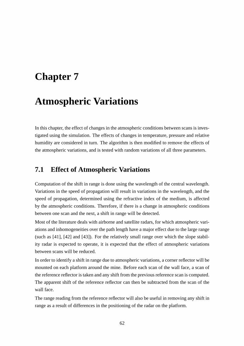
Chapter 7

Atmospheric Variations

In this chapter, the effect of changes in the atmospheric conditions between scans is inves-

tigated using the simulation. The effects of changes in temperature, pressure and relative

humidity are considered in turn. The algorithm is then modified to remove the effects of

the atmospheric variations, and is tested with random variations of all three parameters.

7.1 Effect of Atmospheric Variations

Computation of the shift in range is done using the wavelength of the central wavelength.

Variations in the speed of propagation will result in variations in the wavelength, and the

speed of propagation, determined using the refractive index of the medium, is affected

by the atmospheric conditions. Therefore, if there is a change in atmospheric conditions

between one scan and the next, a shift in range will be detected.

Most of the literature deals with airborne and satellite radars, for which atmospheric vari-

ations and inhomogeneities over the path length have a major effect due to the large range

(such as [41], [42] and [43]). For the relatively small range over which the slope stabil-

ity radar is expected to operate, it is expected that the effect of atmospheric variations

between scans will be reduced.

In order to identify a shift in range due to atmospheric variations, a corner reflector will be

mounted on each platform around the mine. Before each scan of the wall face, a scan of

the reference reflector is taken and any shift from the previous reference scan is computed.

The apparent shift of the reference reflector can then be subtracted from the scan of the

wall face.

The range reading from the reference reflector will also be useful in removing any shift in

range as a result of differences in the positioning of the radar on the platform.

62

0 5 10 150

0.05

0.1

0.15

0.2

0.25

Scans of the Reference Reflectorat Two Different Temperatures

Ambiguous Range (m)

Mag

nitu

de o

f Res

pons

e

308 K 313 K

Figure 7.1: Range Profiles of the Reference Reflector

7.2 Simulation of a Corner Reflector

The corner reflector is modeled as a point target at a range of 202 m, so that it is set back

from the edge of the mine by 2 m. The SNR of the corner reflector will be much higher

than the SNR of the scans of the wall face as the corner reflector focuses the signal back

to the radar. The response of the reference reflector is calculated and processed using

the same methods described in Chapter 3. Range profiles of two scans of the reference

reflector, with a difference in temperature of 5 K between them, are shown in Fig. 7.1.

7.3 Simulation of a Change in Atmospheric Conditions

Variations in atmospheric conditions result in a change in the refractive index of the air.

This changes the speed of propagation of the radar signal which results in a change in the

63

wavelength of the central frequency. The wavelength of the central frequency is calculated

using

λcentral =c

fcentral

(7.1)

wherec is the speed of propagation of the signal, andfcentral is the central frequency.

The speed of propagation is calculated usingclight

n, whereclight is the speed of light in a

vacuum andn is the refractive index of the medium. Sincen is generally very close to

unity, radio refractivityN is defined as

N ≡ (n− 1)× 106 (7.2)

N is dependent on the temperature, pressure and partial pressure of water vapour of the

medium. It is calculated using

N = 77.6

(P

T

)+ 3.73× 105

( e

T 2

)(7.3)

whereP is the air pressure in millibars,T is the temperature in Kelvin ande is the partial

pressure of water vapour [44, Chapter 8].

The simulation has default values for the temperature, pressure and partial pressure of

water vapour for the first scan. The user then enters the change in each of the variables

for the second scan.

The independent effect of each of these three variables on the range calculation of the

reference reflector is now considered in turn.

7.3.1 Change in Temperature

The default temperature in the simulation for the first scan is35oC, as the Limpopo

Province in South Africa is generally a hot region. The user enters the change in tem-

perature between scans, and the effect on the central wavelength is calculated using the

equations given. The simulation is then used to calculate the apparent shift in range of the

reference reflector with various changes in temperature between scans. The graph of the

results of the simulation is given in Fig. 7.2.

It can be seen from the graph that the relationship between temperature and apparent shift

in range is fairly linear. Changes in temperature between scans do not result in large shifts

in range, particularly for small changes in temperature.

64

−35 −30 −25 −20 −15 −10 −5 0 5 10 15 20−20

−15

−10

−5

0

5

10

Apparent Shift in Range of Reference ReflectorDue to Variations in Temperature

Difference in Temperature Between Scans (K)

Shi

ft in

Ran

ge o

f Ref

eren

ce R

efle

ctor

(m

m)

Figure 7.2: Apparent Shift in Range Due to Changes in Temperature

65

−40 −30 −20 −10 0 10 20−1.5

−1

−0.5

0

0.5

1

1.5

2

2.5

Shift in Range due to Pressure Changes Measured Using Reference Reflector

Pressure Difference Between Scans (mbars)

Shi

ft in

Ran

ge B

etw

een

Sca

ns (

mm

)

Figure 7.3: Apparent Shift in Range Due to Changes in Pressure

7.3.2 Change in Pressure

The default pressure for the first scan in the simulation is 1000 mbars. The user enters the

change in pressure between the two scans. The apparent shift in range for various changes

in pressure between two scans is shown in Fig. 7.3.

As with temperature, the relationship between pressure change and apparent shift in range

of the reference reflector is fairly linear. However, a change in pressure between scans

results in a very small apparent shift in range.

7.3.3 Change in Partial Pressure of Water Vapour

Dalton’s law of partial pressure states the following:

“For a mixture of gases in a container, the total pressure exerted is the sum of

66

all the partial pressures of the gases present. The partial pressure of a gas is

the pressure that the gas would exert if it were alone in the container”. [45]

Therefore the partial pressure of water vapour is simply a measure of the water vapour

content of the air.

Relative humidity is commonly used as a measure of the amount of water vapour in the

air. It is defined as the ratio of the actual amount of water vapour in the air to the amount

it could hold when saturated, and is expressed as a percentage [46]. The partial pressure

of water vapour,e, is related to the relative humidity as follows:

e =rh

100exp[−6096.9385

T+21.2409642− 2.711193∗T

100+ 1.673952∗T2

105+2.433502log(T )] (7.4)

whererh is the relative humidity expressed as a percentage,T is in Kelvin, ande is

calculated in millibars [47].

It can be seen from the equation thate is relative to the temperatureT , since the amount

of water vapour the air can hold increases with temperature. A graph of the variation ofe

with relative humidity, calculated using the given equation, is shown in Fig. 7.4 for three

different temperatures.

The default value for relative humidity in the simulation is 50%. The user enters the

difference in relative humidity between the two scans. The apparent shift in range of the

reference reflector for various changes in relative humidity is shown in Fig. 7.5. Since

the partial pressure of water vapour is also dependent on temperature, three different

temperatures are considered.

The relationship between the change in the partial pressure of water vapour between scans

and the apparent shift in range is fairly linear. A change in the partial pressure results in

only a small apparent shift in range, even at high temperatures.

7.4 Variation of Atmospheric Effects With Range

The reference reflector is at a range of 202 m. For a scan of a large section of the wall

face, the range to the centre of each cell might differ greatly from 202 m. Therefore the

relationship between the effect of the atmospheric variations and the range of the reading

needs to be known.

This is done using the simulation by changing the angle of the wall face from30o, as

shown in Fig. 5.1, to72o. This introduces a large variation in range to the centre of

each cell. A difference in temperature of30oC between scans is used, as variations in

67

0 10 20 30 40 50 60 70 80 90 1000

0.5

1

1.5

2

2.5

3

3.5

4

4.5

Variation of the Partial Pressure of Water VapourWith Relative Humidity

Relative Humidity (%)

Par

tial P

ress

ure

of W

ater

Vap

our

(mba

rs)

Temperature = 20 deg CTemperature = 35 deg CTemperature = 50 deg C

Figure 7.4: The Partial Pressure of Water Vapour Modeled Using Relative Humidity

68

−50 −40 −30 −20 −10 0 10 20 30 40 50−2

−1.5

−1

−0.5

0

0.5

1

1.5

2

Apparent Shift in Range of Reference ReflectorDue to Variations in Partial Pressure of Water Vapour

Difference in Relative Humidity Between Scans (%)

App

aren

t Shi

ft in

Ran

ge o

f Ref

eren

ce R

efle

ctor

(m

m)

Temperature = 20 deg CTemperature = 35 deg CTemperature = 50 deg C

Figure 7.5: Apparent Shift in Range Due to Variations in the Partial Pressure of Water

69

Table 7.1: The Variation of Atmospheric Effect With Range

Range to Centre (m) Apparent Shift (mm)

Reference Reflector 202 2.64Cell a3 147 1.95Cell b3 130 1.71Cell c3 117 1.57

temperature have the largest effect on range calculations. The actual shift of the wall face

between scans is zero, so any apparent shift in range is due only to atmospheric variations.

Table 7.1 shows the range to the centre of each cell and the apparent shift introduced by

the increase in temperature of30oC. From the figures shown in the table, the effect of the

increase in temperature on cells at different ranges is approximately 0.013 mm per metre

change in range. The relationship is assumed to be linear as the relationships between

changes in temperature, pressure and the partial pressure of water vapour and apparent

shifts are all linear.

This variation with range could be a source of errors for scans in which the ranges to the

centres of the cells differs greatly from the range to the reference reflector. A difference

in range of approximately 35 m is required for a resultant error of 0.5 mm. Therefore, an

apparent shift in range of the reference reflector needs to be modified relative to the range

to the centre of each cell in order to accurately correct for atmospheric variations.

This necessitates a rough range reading for each cell of the scan, and for the reference

reflector. A range reading for the reference reflector can be obtained fairly easily using

GPS. Range readings for the centre of each cell of the scan can be estimated using a rough

3-d mapping of the mine that has already been carried out using GPS. These ranges need

only be accurate to approximately 5 m.

7.5 Updated Algorithm

In the simulation, noise is added to the range of the reference reflector in order to simulate

an inaccuracy in the measurement of± 30 cm. The range to the centre of each cell

of the scan is computed using simple geometry, and then noise is added to simulate an

inaccuracy of± 2 m. Then for each cell of the scan, the shift in range due to atmospheric

variations is calculated using the simple ratio

shiftcell =rangecell

rangeref

∗ shiftref (7.5)

70

Table 7.2: Change in Atmospheric Conditions Between the Two Scans

Temperature (oC) Pressure (mbars)Relative Humidity (%)

Scan 1 35 1000 50Scan 2 15 - 55 960 - 1040 0 - 100

whererangecell is the range to the centre of the cell,rangeref is the range to the reference

reflector, andshiftref is the apparent shift of the reference reflector.

The value ofshiftcell for each cell of the scan is subtracted from the shift calculated for

that cell.

7.6 Results of the Simulation

The simulation was altered so that a random change in temperature, pressure and relative

humidity occurred between scans, as shown in Table 7.2. The simulation was then run for

various shifts in range of the wall face. As in Chapter 5, only a mass movement of the

cells is considered. The changes in the atmospheric conditions and the errors recorded for

cells b2, b3 and b4 are shown in Table 7.3.

As can be seen in the table, the algorithm performed well within the specified precision,

even with large variations in atmospheric conditions. The largest error was 0.25 mm.

7.7 Conclusion

In this chapter, the effects of changes in atmospheric conditions between scans was inves-

tigated. It was found that atmospheric variations between scans resulted in an apparent

shift of range which was not due to a shift of the wall face, and was therefore a poten-

tial source of error. The apparent shifts, however, were not large, even for significant

changes in atmospheric conditions. The algorithm was updated in order to remove this

apparent shift, with the requirement of a rough range reading to the centre of each scan,

and performed satisfactorily with no significant errors being recorded.

There are two practical possibilities for the scanning procedure of the slope stability radar

in order to reduce the magnitude of potential atmospheric changes between scans, thereby

reducing the possibility of an error:

1. Scans from a particular platform should be taken at the same time each day. At-

mospheric conditions at the same time of day are less likely to differ by a large

71

Table 7.3: Errors in Cells b2, b3 and b4 for Random Atmospheric VariationsRange Shift ∆Temp. ∆Press. ∆Rel. Humidity Shift of Ref. Error for Error for Error for

(mm) (oC) (mbars) (%) Reflector (mm) Cell b2 (mm) Cell b3 (mm) Cell b4 (mm)

0 18 -12 8 2.23 -0.04 -0.10 -0.091 25 -20 21 2.34 0.02 0.08 0.032 19 -28 2 3.35 -0.17 -0.11 -0.013 15 12 16 0.48 -0.03 0.04 -0.004 6 -11 31 0.57 -0.10 -0.06 -0.005 21 -13 -29 3.89 -0.08 -0.11 0.006 -16 -26 11 -1.02 0.19 -0.04 -0.077 -21 -27 4 -1.69 -0.09 -0.01 0.108 -23 -15 -22 -2.61 0.10 -0.01 0.179 3 13 30 -0.95 0.07 0.25 0.0610 14 -39 -2 3.49 -0.05 0.07 -0.0211 20 38 -42 1.86 0.05 -0.14 0.0812 -12 34 49 -3.90 0.08 0.09 0.0113 -20 15 27 -3.91 -0.11 -0.18 -0.1814 -20 12 10 -3.76 0.05 0.07 0.1115 -21 1 -2 -3.34 0.11 0.05 0.05

amount.

2. Scans can be taken continuously from one platform for a given period of time, as

was suggested in the conclusions of Chapter 6. At the beginning of each scan, a

measurement of the reference reflector is taken and corrected for. The atmospheric

variations over this small time scale can be expected to be minimal.

72

Chapter 8

Conclusions

8.1 Review of the Thesis

The objective of this thesis was to assess the suitability of a radar as a slope stability

technique for an opencast mine. The proposal was to mount the radar on a platform on

the rim of the mine, in order to monitor the opposite wall face and detect any movement,

to a specified precision of 1 mm.

The objective was achieved by developing an application-specific simulation of the radar.

This simulation was used to develop the algorithm to monitor the wall face and detect

any shift, using appropriate signal processing techniques, and to investigate possible error

sources.

Differential interferometry was used as the basis of the algorithm to calculate the shift in

range of the wall face, in which a difference in range between the two scans translates to

a difference in phase. The inherent ambiguity in the phase difference was solved using

phase correlation to calculate the gross shift, which is the integer number of wavelength

shifts between scans (14.2 mm). The simple scenario of a single cell of a scan was simu-

lated, and the algorithm was found to perform well within its specified precision.

In order to test the algorithm using this simple scenario, real readings were taken of a wall

using a radar that had been built at the University of Cape Town. A number of differences

existed between the parameters of the real radar and the proposed parameters of the slope

stability radar, notably the frequency range and the beamwidth of the antennas. The

effects of these differences on the readings were taken into account, and the algorithm

then calculated the changes in range within the expected accuracy, with the exception of

a small number of the readings. The ability of the algorithm to calculate the shift in range

for real data demonstrated two things:

73

1. The algorithm worked as expected;

2. The simulation provided realistic data and was therefore a suitable platform on

which to develop and test the algorithm.

The simulation was then expanded to generate data for the full scan of a wall face - five

cells in azimuth and three in elevation. A mass movement of the wall face towards the

radar was simulated as a simple pattern of movement. The algorithm performed well

within its specified precision, with the exception of a small number of gross shift errors.

These were found to occur at shifts in range which were in the region of an odd integer

multiple of the half-wavelength (7 mm, 21 mm, 35 mm...). At these shifts in range, the

peak of the correlation curve, which is used to calculate the gross shift, lies between

two indeces. Therefore its exact position is difficult to resolve and an error of one half-

wavelength may occur. No gross shift error occurred for any shift in range of less than 6

mm.

The simulation was then used to generate data for more complicated patterns of shifting.

This was done in order to investigate the first expected source of error - temporal decorre-

lation. This occurs when the geometric arrangement of scatterers within a cell is changed

between scans, resulting in a change in the backscattering characteristics of that cell so

that direct comparison of the phase values becomes less meaningful. The magnitude of

the peak of the phase correlation curve was used as a measure of the correlation between

scans, or a confidence value of the measurement. Three patterns of shifting were simu-

lated - a change in angle, a localised shift within a cell, and a wedge failure. It was found

that temporal decorrelation did result in errors in the calculated shift in range, and that

the confidence value was a useful indicator of the extent of decorrelation between scans.

For small shifts in range, up to 6 mm, the maximum error was 2 mm (i.e. a precision of 4

mm).

Changes in the atmospheric conditions between scans, resulting in a change in the wave-

length of the radar signal, was the other expected source of error. Changes in temperature,

pressure and the relative humidity were simulated in turn, and temperature was found to

result in the largest error. It was proposed that a corner reflector be mounted on the plat-

form on the rim of the opposite wall face, in order to take a reference reading to calculate

the apparent shift between scans introduced by atmospheric variations. This reference

reading was included in the simulation, and the algorithm was modified to remove the

calculated apparent shift. The magnitude of the apparent shift was shown to be relative

to the range of the reading, so the range to the centre of each cell needs to be known to

an accuracy of approximately 5 m. The simulation was run with random variations of

the atmospheric conditions, and the apparent shift, relative to the range of each cell, was

74

removed. The modified algorithm successfully removed the apparent shift and performed

well within the specified precision

8.2 Summary of the Results

1. The algorithm performed extremely accurately as an indicator of zero shift between

scans.

2. The algorithm performed within specifications for a mass movement of the wall

face, i.e. a simple translational shift. Gross shift errors occurred for certain shifts in

range which were close in value to an odd integer multiple of the half-wavelength,

i.e. 7 mm, 15 mm, 21 mm and so on. No gross shift errors occurred for shifts of

less than 6 mm.

3. Temporal decorrelation does result in significant errors. Intuitively, the precision

of the measurement decreases as the magnitude of the shift increases. The con-

fidence value provides an indication of the extent of decorrelation between scans,

and therefore the accuracy of the calculated shift. The simulation of a wedge failure

combined a mass movement, changes in angle and localised shifts, and is a com-

mon pattern of failure. The main results of the algorithm for a wedge failure were

as follows:

(a) For shifts in range of less than 7 mm, all readings had errors of less than 2

mm.

(b) For shifts in range from 7 to 10 mm, down to a confidence value of 0.6, gross

shift errors were recorded for a small number of readings but fine shift errors

remained less than 2 mm.

4. The effect of changes in atmospheric conditions between scans can be calculated

and corrected for using a reference reflector.

8.3 Final Assessment of Technique

Based on the results of the simulation, the following assessment of the technique is made:

1. It is very accurate as an indicator of zero movement of the wall face.

75

2. It performs within the specified precision of 1 mm for small movements (less than

2 mm). Therefore if the time period between scans is short, the technique is very

accurate, as larger shifts are unlikely.

3. For larger movements, or for a longer time period between scans (24 hours), the

technique detects that a shift has occurred. However, the accuracy of the calculation

is dependent on the nature of the shift. The confidence value provides an indicator

of this accuracy.

8.4 Recommended Scanning Procedure

1. Study the layout of the mine. Determine positions of platforms in order to minimise

their number and maximise the coverage of the wall face.

2. Calculate the azimuth and elevation angles for each cell of a scan from one platform.

Calculate the ranges from the platform to the centre of each cell, using GPS readings

and simple geometry, to an precision of 5 m. This is required for accurate removal

of atmospheric effects.

3. Mount a corner reflector on the front of each platform, in order to enable the radar

on the opposite side of the mine to use it as a reference reflector.

4. Scan continuously from one platform for a period of a day or half a day - this is

to be decided by the mining engineers depending on the rate at which they expect

movement to occur. Errors introduced by temporal decorrelation are likely to be

very small over the short time period between scans. The actual time taken for a

full scan depends on the number of cells which make up the scan, the time taken to

get a reading for each cell, and the speed of the directional motor of the radar

5. The scanning procedure is as follows:

(a) Take a scan of the reference reflector which is mounted on the front of the

platform on the other side of the mine. This scan is compared to the previous

scan and to the first scan of the session from that particular platform. The first

scan of a session is compared to a scan from the previous session.

(b) Scan the opposite wall face. As was the procedure for the reference reflector,

each cell of the scan is compared to the previous scan and to the first scan of

the session.

6. The algorithm will output the following:

76

(a) The calculated shift in range for each cell. This is the average shift of scatter-

ers which make up the cell in the direction of line-of-sight of the radar.

(b) The confidence value. This is an indication of the amount of temporal decor-

relation that has occurred between scans, and of the precision of the calculated

shift.

77

Bibliography

[1] Jami M.Girard and Ed McHugh, "Detecting Problems With Mine Slope Stability"

www.cdc.gov/niosh/mining/pubs/pdfs/dpwms.pdf , National Institute

for Occupational Safety and Health, Spokane Research Laboratory.

[2] W.F. Kane, "Development of a Time Domain Reflectometry System to Mon-

itor Landslide Activity: Final Report" www.iti.northwestern.edu/

publications/tdr/kane/old_kane/lane_ch1.html , 1996.

[3] Dr. A.J. Mendecki et al, “Seismology for Rockbursts Prevention, Control and Predic-

tion”, ISS International Ltd, SIMRAC Project GAP 017, 1996.

[4] A.v.Z Brink et al, “Survey And Assessment Of Techniques Used to Quantify The Po-

tential For Rock Mass Instability”, CSIR: Division of Mining Technology, SIMRAC

Project GAP 608, 2000.

[5] "Application Note: Non-contact Laser Distance Measurement"www.

lasercomponents.de/wwwe/pdf/distmeas.pdf , Laser Components

GmbH, Werner-von-Siemens-str. 15, D-82140 Olching.

[6] "Long-Range Measuring System LPM-2K"www.riegl.co.at/lpm_ptm/e_

lpm-2k.htm , RIEGL Laser Measurement Systems, Austria, 2002.

[7] Glenn Egan, "Comparison of Industrial Measurement Techniques"www.gmat.

unsw.edu.au/final_year_thesis/Egan?EGAN’rev.htm , School of

Surveying and Spatial Information Systems, University of New South Wales, 2002.

[8] John Tyson and Timothy Schmidt, "Advanced Photogrammetry for Robust Deforma-

tion and Strain Measurement"www.trilion.com/Ppr.204.SEM.350.sm.

pdf , Trilion Quality Systems LLC, Germany.

[9] P. Collier, L. Dixon, D. Fontana, D. Payne and A.W. Pearson, "The Use of

Close Range Photogrammetry for Studying Ice Accretion on Aerofoil Sections"

78

snap.lut.ac.uk/PhotoSoc/abs/phroct99/Collier.pdf , University

of Portsmouth, Photogrammetric Record, 16(94), 1999, pp.671-684.

[10] A. Langman, M. Inggs, “A Stepped Frequency CW Polarimetric Radar for Mine

Detection”, Journal of the Eurel International Conference on Detection of Abandoned

Landmines, Number 431, pp 109-113, October 1996.

[11] B. Reeves, D. Noon, G. Stickley and D. Longstaff, "Highwall Stability Monitoring

Radar"www.cssip.uq.edu.au/highwall/highwall.html , University of

Queensland, Australia, 2002.

[12] "Slope Stability Radar" www.groundprobe.com/PDF/SSR_Brochure.

pdf , Groundprobe, Australia, 2002.

[13] B. Reeves, D. Noon, G. Stickley and D. Longstaff, "Slope Stability Radar for

Monitoring Mine Walls" www.ips.gov.au/IPSHosted/NCRS/wars2002/

proceedings/comm-f/screen/noon_e-abs.pdf , extended abstract, Co-

operative Research Centre for Sensor Signal and Information Processing (CSSIP),

School of Information Technology and Electrical Engineering, University of Queens-

land, Australia, 2002.

[14] D.J. Tanser, “The Detection of Land Mines Using Ground Penetrating Radar Data”,

under-graduate thesis, University of Cape Town, 2000.

[15] A. Langman, “Basic Principles of Step Frequency CW GPR”, Radar Remote Sens-

ing Group (RRSG), University of Cape Town, 1997.

[16] A. Langman, “The Design of Hardware and Signal Processing for a Stepped Fre-

quency Ground Penetrating Radar”, PhD thesis, University of Cape Town, 2002.

[17] Donald R. Wehner, “High Resolution Radar”, Artech House, Boston, London, 2nd

edition, 1994.

[18] Chapter 1: High Resolution Radar (HRR) Waveformswww.tele.ntnu.no/

radio/fag/SIE2050/Waveforms.pdf , no name or date available.

[19] C.T. Wang, H.T. Wang, D.C. Chern, N.Y. Chen, L.S. Liang, "A Study on Differen-

tial Interferometry in Subsidence"www.gisdevelopment.net/aars/acrs/

2000/ts14/sari0004.shtml , proceedings of the Asian Conference on Re-

mote Sensing, Taipei, Taiwan, 2000.

79

[20] F. Rocca, C. Prati and A. Ferretti, "An Overview of Sar Interferometry"earth.

esa.int/symposia/program-details/speeches/rocca-et-al ,

Earthnet Online, European Space Agency, 2002.

[21] G.X. Liu, Y.Q. Chen, X.L. Ding, Z.L. Li and Z.W. Li, "Monitoring Ground

Settlement in Hong Kong with Satellite SAR Interferometry"www.fig.net/

figtree/pub/fig_2002/Js17/JS17_liu_etal.pdf , Hong Kong Poly-

technic University, Hong Kong, China, 2002.

[22] Maurice Borgeaud, Eoropean Space Agency, and Urs Megmueller, GAMMA Re-

mote Sensing AG, "On the Use of ERS SAR Interferometry for the Retrieval

of Geo- and Bio-Physical Information"www.geo.unizh.ch/rsl/fringe96/

papers/borgeaud-wegmueller/ , ERS SAR Interferometry Workshop, Uni-

versity of Zurich, 1996.

[23] A. Gkoufa, N. Sifakis, N. Soulakellis, "Use of SAR interferometry to derive ad-

ditional information on the surface roughness and DEM"mara.jrc.it/pdf/

sarinterferometry.pdf , National Observatory of Athens, Institute for Space

Applications and Remote Sensing, 1998.

[24] Christopher T. Allen, Iinterferometric Synthetic Aperture Radar"

www.ittc.ukans.edu/publications/documents/Allen1995_

Allen1995GRSSNpp6.pdf , review article for the Department of Electrical Engi-

neering and Computer Science and Radar Systems and Remote Sensing Laboratory,

University of Kansas, 1995.

[25] Earthnet Online, "SAR Interferometry"earth.esa.net/0xc1cce41c_

0x000002cb , European Space Agency, 2002.

[26] H.A. Zebker, J. Villesanor, Jet Propulsion Laboratory, “Decorrelation in Interfero-

metric Radar Echoes”, IEEE Transactions on Geoscience and Remote Sensing, 30(5),

pp.950-959, 1992.

[27] Peter Wittenberg, "Introduction to Airborne Radar"home.att.net/

~wittenberg/radar/chapters/ch12.dir/ch12pr.dir/c12p7.

dir/c12p7.htm , Scitech Publishing Inc, 1997.

[28] F.G. Stremler, “Introduction to Communication Systems”, Addison-Wesley Publish-

ing Company, Reading, Massachusetts, 3rd edition, 1990.

80

[29] Julius O. Smith III, "Zero Padding"ccma-www.stanford.edu/~jos/mdft/

Zero_Padding.html , Center for Computer Research in Music and Acoustics

(CCRMA), Stanford University, 2003.

[30] Richard G. Lyons, "How to Interpolate in the Time-Domain by Zero-Padding in

the Frequency Domain"www.dspguru.com/howto/tech/zeropad2.htm ,

Iowegian’s dspGuru, 1999.

[31] A.J. Wilkinson, “Lecture Notes on Radar Signal Processing”, Class notes for the

MSc radar signal processing course, University of Cape Town, 2002.

[32] Yi Liang, "Phase-Correlation Motion Estimation"ise.stanford.edu/

class/ee392j/projects/liang_report.pdf , EE 392J Final project,

Stanford University.

[33] J.P. Lewis, "Fast Normalized Cross-Correlation"citeseer.nj.

nec.com/cache/papers/cs/23041/http:zSzzSzwww.idiom.

comzSz~zillazSzWorkzSznvisionInterfacezSznip.pdf/

lewis95fast.pdf , Industrial Light and Magic, 1995.

[34] Lyndon Hill, "Phase Correlation"www.ee.surrey.ac.uk/Personal/L.

Hill/pc.html , under supervision of Theo Vlachos, University of Surrey, 2000.

[35] C.D. Kuglin, D.C. Hines, “The Phase Correlation Image Alignment Method”, Pro-

ceedings of the IEEE International Conference on Cybernetics and Society, New

York, NY, pp 163-165, 1975.

[36] James C. Tilton, "Comparison of Registration Techniques for GOES Visible

Imagery Data"code935.gsfc.nasa.gov/code935/tilton/goes_reg/ ,

Applied Information Sciences Branch, NASA’s GSFC, no year available.

[37] Merrill Skolnik, "Integration of Radar Pulses"www.engr.ucf.edu/centers/

cfrsl/integ_of_radar_pulse_revC.pdf , Introduction to Radar Systems,

3rd edition, no year available.

[38] Special Study Group 2.160, "SAR Interferometry Technology"www.gfy.ku.dk/

~iag/Travaux_99/ssg2160.htm , XXII IUGG General Assembly, Birming-

ham, 1999.

[39] R. Romeiser and D.R. Thompson, "Study on Concepts for Radar Interferometry

from Satellites for Ocean (and Land) Applications"www.ifm.uni-hamburg.

81

de/!wwwrs/modeling/data/koriolis_sect2.pdf , KoRIOLiS Report,

Section 2: Fundamentals, no year available.

[40] Laurent Meunier and Moritz Borgmann, "High-Resolution Panoramas Using Image

Mosaicing" ise0.stanford.edu/class/ee368a_proj00/project13/

registration.html , Stanford University, 2000.

[41] R. Hanssen, Delft University of Technology, and A. Feijt, Royal Netherlands Mete-

orological Institute, "A first quantitative evaluation of atmospheric effects on SAR

interferometry"www.geo.unizh.ch/rsl/fringe96/papers/hanssen/ ,

ERS SAR Interferometry Workshop, University of Zurich, 1996.

[42] Z.W. Li, X.L. Ding, G.X. Liu, Y.Q. Chen, Z.L. Li and J.J. Zhu, "Study of Atmo-

spheric Effects on Satellite Synthetic Aperture Radar (SAR) Measurements in Trop-

ical Regions"wwww.ddl.org/figtree/pub/fig_2002/Js17/JS17_li_

etal.pdf , JS17 Special Sensors and Techniques in Engineering Surveys, China.

[43] G. Linlin, T. Tsujii and C. Rizos, "Tropospheric Heterogeneities Correc-

tions in Differential Radar Interferometry"www.gmat.unsw.edu.au/snap/

publications/ge_etal2002a.pdf , University of New South Wales, Sydney,

Australia, 2002.

[44] S. Kingsley and S. Quegan, “Understanding Radar Systems”, Scitech Publishing

Inc., Mendham, New Jersey, 1999.

[45] Jim’s DemoCam, "Dalton’s Law"www.d230.org/jod/gas/new_page_4.

htm , no author or date available.

[46] "Humidity Calculator"www.bom.gov.au/lam/humiditycalc.shtml , Bu-

reau of Meteorology, Commonwwealth of Australia, 2003.

[47] "Partial water vapour pressure (dew point)"www.npl.co.uk/ssfm/metros/

key_functions/properties/partial_water_vapour_pressure_

dew_point/ , National Physical Laboratory, Teddington, Middlesex, UK, 2000.

82

Appendix A

Simulation of a Single Cell of a Scan

83

Appendix B

Processing of Real Data Using the

Algorithm

88

Appendix C

Expanded Simulation of an Entire Scan

92

simulation of a slope stability radar for opencast...

Documents