simulation of fluid catalytic cracking with single-event
TRANSCRIPT

Universiteit GentFaculteit Ingenieurswetenschappen
Vakgroep Chemische Proceskunde en Technische ChemieLaboratorium voor Petrochemische Techniek
Directeur: Prof. Dr. ir. G.B. Marin
Simulation of Fluid Catalytic Cracking
with Single-Event MicroKinetics and
Computational Fluid Dynamics
Pieter Lagaert
Prof. Dr. ir. G. HeynderickxProf. Dr. ir. G.B. Marin
Promotoren
Ir. E. BaudrezBegeleider
Master thesis ingediend tot het behalen van de academischegraad van Burgerlijk Scheikundig Ingenieur
Academiejaar 2006–2007

Universiteit GentFaculteit Ingenieurswetenschappen
Vakgroep Chemische Proceskunde en Technische ChemieLaboratorium voor Petrochemische Techniek
Directeur: Prof. Dr. ir. G.B. Marin
Simulation of Fluid Catalytic Cracking with Single-EventMicroKinetics and Computational Fluid Dynamics
Pieter Lagaert
Prof. Dr. ir. G. HeynderickxProf. Dr. ir. G.B. Marin
Promotoren
Ir. E. BaudrezBegeleider
Master thesis ingediend tot het behalen van de academische graad vanBurgerlijk Scheikundig Ingenieur
Academiejaar 2006–2007
Chapter 1 contains a short description of the Fluid Catalytic Cracking processand the specification of the goal of this master thesis. The remainder of thereport has been divided in four parts. The first part consists of a literature sur-vey about numerical solution techniques for reactive flows. Different acceptednumerical techniques with their corresponding (dis-)advantages are presentedin chapter 2. The second part describes of the kinetic and hydrodynamic modelused to perform the simulations. Chapter 3 describes the single-event kineticmodel that is used to simulate the reactions in the riser. In chapter 4, a discus-sion concerning the stiffness of the kinetic model is presented. This discussionresults in the selection of a suitable solver for the integration of the reactionpart in the transport equations. Chapter 5 contains an overview of the modelequations and constitutive laws on which the simulations are based. A programwas developed to integrate the transport equations for each reactive componentand the general principles of this program are given in chapter 6. The simula-tion results are presented in the third part. Chapter 7 describes the input datafor the simulations, the simulation results and a comparison with other simu-lations from literature. Chapter 8 presents the conclusions of this master thesisand suggestions for future work. The last part of the report consists of the ap-pendices. In Appendix A, a summary of the model equations is given. AppendixB contains the input data that have been used to perform the simulations.
I
___________________________________________________________________________________________ Krijgslaan 281 S5, B-9000 Gent (Belgium)
tel. +32 (0)9 264 45 16 • fax +32 (0)9 264 49 99 • GSM +32 (0)475 83 91 11 • e-mail: [email protected]
http://allserv.ugent.be/tw12/
Opleidingscommissie Scheikunde
Verklaring in verband met de toegankelijkheid van de scriptie
Ondergetekende, Lagaert Pieter
afgestudeerd aan de UGent in het academiejaar 2006-2007 en auteur van de scriptie
met als titel:
Simulation of Fluid Catalytic Cracking with Single-Event MicroKinetics and
Computational Fluid Dynamics
verklaart hierbij:
1. dat hij/zij geopteerd heeft voor de hierna aangestipte mogelijkheid in verband
met de consultatie van zijn/haar scriptie:
de scriptie mag steeds ter beschikking gesteld worden van elke aanvrager
de scriptie mag enkel ter beschikking gesteld worden met uitdrukkelijke,
schriftelijke goedkeuring van de auteur
de scriptie mag ter beschikking gesteld worden van een aanvrager na een
wachttijd van jaar
de scriptie mag nooit ter beschikking gesteld worden van een aanvrager
2. dat elke gebruiker te allen tijde gehouden is aan een correcte en volledige
bronverwijzing
Gent, 04-06-2007
Lagaert Pieter
FACULTEIT TOEGEPASTE WETENSCHAPPEN
Chemische Proceskunde en Technische ChemieLaboratorium voor Petrochemische Techniek
Directeur: Prof. Dr. Ir. Guy B. Marin

Simulation of Fluid Catalytic Cracking withSingle-Event MicroKinetics and Computational
Fluid DynamicsPieter Lagaert
Promoters: Prof. Dr. ir. G. Heynderickx and Prof. Dr. ir. G.B. MarinCoach: Ir. E. Baudrez
Abstract— A three-dimensional gas-solid simulation of theriser of a catalytic cracking unit is presented. In orderto perform these simulations, a complex kinetic model hasbeen combined with a complete three-dimensional hydrody-namic model. The kinetic model has been developed at theLaboratorium voor Petrochemische Techniek at the Univer-sity of Ghent. Because of the fundamental character of thisSingle-Event MicroKinetic model, the rate coefficients arefeed-independent. The individual transport equations forthe gas phase components and cokes have been integratedby applying a first-order operator splitting technique. Inthis method, the convection part and the reaction part ofthe transport equations are solved separately in a two-stepsequence. The simulation results correspond well with sim-ulation results presented in literature.
Keywords: FCC, 3D simulation, Single-Event MicroKineticmodel, operator splitting, stiffness, riser reactor
I. INTRODUCTION
The Fluid Catalytic Cracking (FCC) unit is the primary con-version unit in modern oil refineries. In this process, a low-valueheavy crude oil feed is cracked into lighter and higher-valueproducts that can be used for transportation fuel (gasoline anddiesel).In this work, a CFD simulation of the riser section of a catalyticcracking unit has been performed. While most Fluid CatalyticCracking simulations rely on kinetic models using drastic lump-ing or on simple hydrodynamic models, in this work a detailedfundamental kinetic model is combined with a complete three-dimensional hydrodynamic model.
II. SINGLE-EVENT MICROKINETIC MODEL
In order to describe the complex cracking reactions whichtake place in the riser, the Single-Event Microkinetic Model isapplied in this work. The basics of this model have been devel-oped by Froment, Vynckier and Dewachtere [1]. As a last step,Quintana-Solorzano et al. [2] have extended the kinetic modelwith fundamental prediction of coke formation. All reactantsand products are grouped in 678 lumps. The 678th componentconsists of the coke which is formed on the catalyst. The globalreaction rate of each lump is based explicitly on the elementaryreaction steps of the carbenium ions involved in the conversionfrom reactant to product. Since these elementary reaction paths
have a fundamental character, the reaction rate coefficients ofthe single-event model remain independent of the feed compo-sition.
III. HYDRODYNAMIC MODEL
The applied hydrodynamic model consists of the continuity,momentum, energy and turbulence balances for both the gas andthe solid phase, closed with a number of constitutive relations.The model is completed by the continuity equations for the gasphase components and the coke that deposits on the catalyst.The model equations are partially solved by the commercialsimulation package Fluent and partially by a user defined pro-gram, that interacts with Fluent. As the number of componentsin the Single-Event MicroKinetic model exceeds the maximumnumber of continuity equations that can be solved by Fluent, theindividual continuity equations have been solved externally withregard to Fluent.Based on a literature survey, a first-order operator splitting tech-nique [3] has been selected to integrate the gas phase compo-nents transport equations. In this method, the convection partand the reaction part of the transport equations for each gasphase component i are solved separately in a two-step sequence:
Step 1:∂
∂t(εgρgωi) =
1V
[K∑k
[ωup
i (εgρgu · S)]
k
](1)
Step 2:∂
∂t(εgρgωi) = Ri(ω) (2)
The convection part has been discretized with a first-order up-wind method and is integrated with a first-order explicit Eu-ler method. The reaction step is integrated with the stabilizedRunge-Kutta solver [4], which has been selected on the basisof its superior efficiency in comparison with other integrationmethods.
IV. RESULTS AND DISCUSSION
The riser geometry was taken from [5] and as the catalystinlet lies in a plane perpendicular to the gas oil feed nozzles, thesimulations have a three-dimensional character. In Figure 1, thegasoline distribution in two vertical cross sections of the riser ispresented. Lumps with carbon numbers between 5 and 12 havebeen gathered into gasoline to be able to compare these resultswith other three-dimensional simulations from literature.
Figure 1 shows that the mass fraction profiles are not uniformfor low axial coordinates. Temperatures and catalyst concentra-

Fig. 1. Gasoline mass fraction profile in a vertical plane through (i) feed nozzles(ii) catalyst inlet
tions are low near the nozzles because of the injection of the coldfeed, implying low gasoline yields. The highest catalyst concen-trations arise at the catalyst inlet side, resulting in an asymmetricgasoline distribution. As the velocity profiles are less influencedby the feed nozzles and the catalyst inlet higher up in the riser,the production yields become more uniform at these positions.
Figure 2 presents the area averaged conversion and mass frac-tions of HCO, LCO, gasoline, LPG and coke. At the start of thefeed nozzles (3 m), the HCO- and LCO-profiles start to build up.At locations where a combination of high temperature and highcatalyst (fresh!) concentration occurs, the heavy hydrocarbonsthat have entered the riser, crack instantaneously to gasoline.
0,00
0,05
0,10
0,15
0,20
0,25
0,30
0,35
0,40
0,45
0,50
3,0 4,0 5,0 6,0 7,0 8,0 9,0
Axial coordinate [m]
Mas
s fr
acti
on [
kg/
kg g
as]
0,0
0,1
0,2
0,3
0,4
0,5
0,6
0,7
HC
O M
ass
frac
tion
[k
g/k
g gas
]
Gasoline
LCO
LPG
Coke
Conversion
HCO
Fig. 2. Evolution of the area averaged conversion and mass fractions on totalgas phase mass basis of HCO, LCO, gasoline, LPG and coke
While the heavy hydrocarbons are concentrated near the wallbetween 3 and 3.5 m, they are more uniformly spread over the
riser section between 3.5 and 4 m. Once the heavy hydrocar-bons (HCO and LCO) profiles have completely built up (at 4m), LCO and HCO are gradually cracked to gasoline, LPG andcoke. From 3.5 to 6.5 m, specifically LCO is cracked into gaso-line. From 6.5 m on, HCO is cracked to gasoline, LPG, cokeand also LCO.
The profiles obtained in this work correspond well with the sim-ulation results presented in literature. Table I shows that theproduct yields and conversion obtained in this work agree wellwith the corresponding values at comparable riser positions re-ported in literature.
TABLE ICOMPARISON OF THE SIMULATION RESULTS WITH LITERATURE. PRODUCT
YIELDS IN KG/KGGAS .
Gasoline LPG Coke ConversionGao et al. [5] 0.33 0.03 0.02 36%Van Landeghem et al. [6] 0.31 0.01 0.02 46%Das et al. [7] 0.17 0.06 0.025 33%Quintana-Solorzano et al. [2] 0.39 0.06 0.05 52%This work 0.36 0.07 0.027 46%
SymbolsK Total number of cell faces -Ri Net production rate of lump i [kgi/m3
rs]t Time [s]S Cell surface [m2
r]u Velocity vector of the gas phase [m/s]V Cell Volume [m3
r]εg Fraction of the gas phase [m3
g /m3r]
ρg Density of the gas phase [kgg /m3g]
ωi Mass fraction of gas phase species i [kgi/kgg]
REFERENCES
[1] N. V. Dewachtere, F. Santaella, and G. F. Froment, “Application of a Single-Event Kinetic Model in the Simulation of an Industrial Riser Reactor for theCatalytic Cracking of Vacuum Gas Oil,” Chemical Engineering Science,vol. 54, pp. 3653–3660, Aug. 1999.
[2] Roberto Quintana-Solorzano, Joris W. Thybaut, Guy B. Marin, RuneLødeng, and Anders Holmen, “Single-Event MicroKinetics for coke for-mation in catalytic cracking,” Catalysis Today, vol. 107–108, pp. 619–629,2005.
[3] J. G. Blom and J. G. Verwer, “A comparison of integration methods foratmospheric transport–chemistry problems,” Journal of Computational andApplied Mathematics, vol. 126, pp. 381–396, 2000.
[4] B.P. Sommeijer, L.F. Shampine, and J.G. Verwer, “RKC: An explicit solverfor parabolic PDE’s,” Journal of Computational and Applied Mathematics,vol. 88, pp. 315–326, 1998.
[5] J. Gao, C. Xu, S. Lin, G. Yang, and Y. Guo, “Advanced Model for TurbulentGas-Solid Flow and Reaction in FCC Riser Reactors,” AIChE Journal, vol.45, pp. 1095–1113, 1999.
[6] F. Van Landeghem, D. Nevicato, I. Pitault, M. Forissier, P. Turlier, C. Der-ouin, and J.R. Bernard, “Fluid Catalytic Cracking: modelling of an indus-trial riser,” Applied Catalysis A, vol. 138, pp. 381–405, 1996.
[7] Asit K. Das, Edward Baudrez, Guy B. Marin, and Geraldine J. Heynderickx,“Three-Dimensional Simulation of a Fluid Catalytic Cracking Riser Reac-tor,” Industrial and Engineering Chemistry Research, vol. 42, pp. 2602–2617, 2003.

Dankwoord
Mijn appreciatie gaat in de eerste plaats uit naar Edward. Ik zou hem willenbedanken voor zijn programmeer-technische raad, inspirerende ideeen en al detijd dat we samengewerkt hebben. In het bijzonder wil ik hem danken voorzijn enthousiasme, zijn hulpvaardigheid, zijn onvermoeibare motivatie voor mijnwerk en zijn oneindig geduld wanneer het wat minder liep. Ik kon me geen beterebegeleider toewensen! Succes nog met het afronden van je doctoraat!
Verder ben ik Prof. Heynderickx en Prof. Marin erkentelijk voor de kans diezij mij boden om onderzoek te verrichten op dit uitdagende onderwerp. Huninteresse en nuttige richtlijnen werkten als een stimulans voor mij. Prof. Heyn-derickx wil ik nog eens in het bijzonder bedanken voor haar geduld in hetnalezen van mijn teksten.
Uiteraard wil ik al mijn medestudenten van S5 bedanken voor de steun en devele leuke momenten. Dieter, Evelyn, Steven, Hans, Jerry, Jeroen, Jan, Wim,Kim en natuurlijk Sophie: bedankt om steeds naar mij te luisteren en mij op tevrolijken als het wat minder ging! Dank ook aan de andere mensen van BS3, inhet bijzonder aan Kris, Paul en Anneleen.
Aangezien ik door het beeindigen van mijn studies een periode van mijn levenafsluit, is het nu het ideaal moment om de mensen te bedanken die mij gebrachthebben waar ik nu sta en die veel voor mij betekenen.
In de eerste plaats wil ik mijn ouders bedanken. Ondanks niet altijd idealeomstandigheden is hun toewijding naar mij toe onbeschrijflijk. Ik wil hen dankenvoor hun genegenheid, hun verdraagzaamheid, de goede raad en de kansen dieze mij geboden hebben. Verder wil ik mijn broers Bart en Wouter en mijn zusAnnelies bedanken. De ‘kleinen’ heeft veel van jullie geleerd!
Verder wil mijn meme Roos en peter Peter bedanken voor hun steun, huncontinue interesse in mij en voor de centjes die broodnodig waren om het hardestudentleven door te komen. Dank ook aan de rest van mijn familie, in hetbijzonder aan tante Marleen die geen enkel examen vergeten is!
Tenslotte wil ik nog enkele collega-, ex- en niet-burgies bedanken: Benoit, Si-mon, Bart, Willy en Ewoud. Ook dank aan Davy voor de vele pauzekes en devele pintjes. Jullie zijn mijn beste vrienden en ik hoop dat we nog vele mooiemomenten mogen hebben!
V
Samenvatting
De katalytische krakingseenheid is de primaire conversie-eenheid van zwareaardoliefracties in de hedendaagse raffinaderijen. Die zware aardoliefracties wor-den er omgezet tot meer waardevolle lichtere koolwaterstoffen zoals benzine,LPG, enz... De kraakreacties worden uitgevoerd in een verticaal opgesteldebuisreactor, de riser. De vloeibare voeding wordt onderin de riser in contactgebracht met de hete katalysatorkorrels die afkomstig zijn van de regenerator.De voeding verdampt hierdoor en tijdens de opwaartse beweging in de riserworden de gasvormige componenten gekraakt. Bovenaan de buisreactor wordtde katalysator gescheiden van de gasvormige reactieproducten, waarna het ge-vormde nevenproduct cokes dat afgezet werd op de katalysator, afgebrand wordtin de regeneratiesectie van de katalytische kraker.
In deze masterthesis wordt een driedimensionale simulatie van de buisreac-tor in een dergelijke katalytische kraker voorgesteld. Bij het ondernemen vandeze simulatie werd een gedetailleerd kinetisch model gekoppeld aan de com-plexe driedimensionale stromingsvergelijkingen die de reactor hydrodynamicabeschrijven. Dit vormt dan ook de verdienste van dit werk, want de meeste si-mulaties uit de literatuur gaan uit van ofwel een vereenvoudigde kinetiek, ofwelvereenvoudigde reactormodellen.
Numerieke oplossingstechnieken voor tijdsafhankelijke reactievetransportvergelijkingen
Algemeen kan reactieve stroming omschreven worden als een combinatie vanconvectie, diffusie en reactie. Voor iedere component i die beschouwd wordt inhet kinetische model moet bijgevolg volgende transportvergelijking geıntegreerdworden:
∂
∂t(εgρgωi) +∇ · (εgρgωiu) +∇ ·Ji = Ri ∀ i = 1, . . . , N (1)
In dit werk zal de diffusieterm niet beschouwd worden. Dit stelsel vergelijking-en moet voor iedere cel van het 3D oplossingsgrid, waaruit de riserreactor isopgebouwd, opgelost worden. Na discretisatie van de plaatsafgeleiden in deconvectieterm, wordt deze term voor iedere component afhankelijk van zijnconcentratie in buurcellen. Bovendien kan de reactieterm slechts geevalueerd
VI
worden indien de concentraties van alle andere componenten gekend zijn. Hetaantal vergelijkingen dat simultaan moet opgelost worden is dus typisch van degroot-orde van het product van het aantal gridcellen en het aantal beschouwdecomponenten. Indien een complex kinetisch model gebruikt wordt, is de keuzevan een geschikte oplossingsmethode van groot belang. Door middel van eenliteratuurstudie worden de verschillende numerieke oplossingstechnieken voorde tijdsintegratie van de gediscretizeerde versie van (1) onderzocht. De moge-lijkheden worden hieronder summier weergegeven.
In een volledig expliciete integratiemethode worden zowel de reactie- als de con-vectieterm geevalueerd op het lopende tijdsniveau en als een geheel geıntegreerd.Alle vergelijkingen worden op deze manier ongekoppeld opgelost, hetgeen eenaanzienlijke vereenvoudiging van de oplossing met zich meebrengt. Indien de re-actie echter een zekere stijfheid vertoont, moet de expliciete tijdstap klein wor-den gekozen om stabiele integratie te garanderen, hetgeen de rekentijd enormkan doen toenemen.
Een volledig impliciete methode evalueert de reactie- en de convectieterm ophet volgende tijdsniveau. Impliciete methoden kunnen onvoorwaardelijk sta-biel gemaakt worden. Hierdoor kan een grotere tijdstap, die enkel gebaseerd isop accuraatheidsvoorwaarden, toegepast worden. Doordat alle termen op hetvolgende tijdsniveau behandeld worden, moeten de vergelijkingen in de ver-schillende gridpunten en voor iedere component simultaan opgelost worden. Derekentijd wordt zo enorm groot indien een groot aantal componenten beschouwdwordt.
Naast volledig impliciete methoden kunnen ook semi-impliciete methoden ge-bruikt worden. Deze methoden bevatten zowel een impliciet als een explicietdeel. Eerst wordt nagegaan welke termen impliciet moeten behandeld wordenom de stijfheid van het stelsel op te vangen. Indien bijvoorbeeld de convectie-term expliciet wordt geevalueerd, is het aantal vergelijkingen dat simultaandient opgelost te worden beperkt tot het aantal reactieve componenten.
Een laatste categorie oplossingsmethoden zijn de sequentiele oplossingsmetho-den, ook wel ‘operator-’ of ‘time-splitting’ methoden genoemd. Hoewel de fy-sische fenomenen convectie, diffusie en reactie simultaan optreden op elk tijds-niveau, wordt in sequentiele technieken verondersteld dat elk fenomeen sequen-tieel kan geıntegreerd worden in de tijd. De beginvoorwaarde voor elke inte-gratiestap wordt gevormd door de oplossing bekomen in de vorige stap. Devolgorde waarin dit gebeurt, wordt bepaald door het relatieve belang van elkfenomeen. Een speciaal geval binnen deze methoden is de ‘source-splitting’ tech-niek. Hierbij wordt het niet-stijve gedeelte van de transportvergelijking expli-ciet geıntegreerd in een eerste stap. De bijdrage van deze niet-stijve term(en)wordt dan als een constant veronderstelde bronterm bijgeteld in de integratievan het stijve deel. In tegenstelling tot de andere sequentiele methoden, tredenbij ‘source-splitting’ geen discontinuıteiten op omdat de initiele condities voor
VII

beide stappen identiek zijn.
De sequentiele methoden hebben als groot voordeel dat voor elk fysisch feno-meen een geschikte solver kan gekozen worden, hetgeen de flexibiliteit vergroot.Reactie en convectie worden volledig ontkoppeld, waardoor het aantal verge-lijkingen dat simultaan dient opgelost te worden hoogstens van de grootordevan het aantal componenten is. Hierdoor kan de rekentijd enorm dalen indiengepaste numerieke methoden geselecteerd worden voor elk fysisch fenomeen.Het nadeel van de sequentiele techniek is dat een bijkomende numerieke foutoptreedt in de tijdsintegratie als gevolg van de ontkoppeling van de fysischefenomenen, die in werkelijkheid simultaan ageren. Omdat deze fout evenredig ismet de gekozen tijdstap, kan ze gereduceerd worden door voldoende kleine tijd-stappen te kiezen. Operator splitting komt dan ook maar volledig tot zijn rechtindien inherent kleine tijdstappen gebruikt worden omwille van stabiliteits-beperkingen.
Een alternatieve expliciete methode voor het oplossen van de reactieterm in eensequentiele methode is gebaseerd op de Computational Singular Perturbation(CSP) theorie. Deze methode kan slechts toegepast worden indien de snelle entrage tijdschalen, gedefinieerd als de reciproque van de eigenwaarden, in het sys-teem duidelijk onderscheiden zijn. Een nieuw systeem, enkel bestaande uit detrage tijdschalen, kan dan expliciet geıntegreerd worden met een grotere tijdstapomdat het stabiliteitscriterium niet meer gebaseerd is op de snelle modi. Hiernadient wel nog een correctie doorgevoerd te worden die de snelle tijdschalen inrekening brengt. Ondanks het expliciete karakter van deze methode kunnenrekentijden sterk oplopen aangezien op elk tijdsniveau eigenwaarden van de Ja-cobiaan van het systeem en basisvectoren voor de trage modi berekend moetenworden.
Single-Event MicroKinetic Model
Om de complexe kraakreacties die plaatsvinden in de riser te beschrijven, werdin dit werk gebruik gemaakt van het Single-Event MicroKinetisch model. Debasis voor dit model werd gelegd door Froment (1990) en het model werd verdertoegepast op katalytisch kraken door Dewachtere (1997). Quintana-Solorzanoet al. (2005) heeft het model finaal uitgebreid met vergelijkingen die een fun-damentele voorspelling van de cokesvorming toelaten.
De eerste stap in de reactie van een koolwaterstof is de vorming van een carbe-niumion op het katalysatoroppervlak. Deze ionen kunnen vervolgens een aan-tal elementaire reacties ondergaan. Het hierbij gevormde carbeniumion wordtvia deprotonering of hydridetransfer omgezet naar het uiteindelijke koolwater-stofproduct. Het Single-Event MicroKinetisch model brengt deze elementairereactiepaden in rekening via een aantal single-event snelheidscoefficienten. Ditbetekent dat deze snelheidscoefficienten onafhankelijk zijn van de koolwater-stofvoeding, wat impliceert dat het SEMK-model een fundamenteel model is.
VIII
Door het grote aantal mogelijke koolwaterstofcomponenten die op die manierkunnen beschouwd worden, werd het kinetische model gelumpt tot 677 molecu-laire gasfase componenten en coke. De globale reactiesnelheid voor de omzettingvan een lump L1 naar een lump L2 is dan gegeven door de som van de reactie-snelheden van de elementaire stappen die carbeniumionen uit lump L1 omzettentot ionen die desorberen tot moleculen van lump L2.
Het kinetische model werd geımplementeerd in een eendimensionale gas-vastreactorsimulatie (Quintana-Solorzano et al., 2005). Hierbij werd ideale prop-stroming verondersteld voor de gasfase en de vaste fase. Verder was het modelvan pseudo-homogene aard: eenfasig voor de koolwaterstoffen en tweefasig voorde temperatuur. De eendimensionale propstroombalansen werden geıntegreerddoor de LSODA-solver, die automatisch overschakelt tussen stijve en niet-stijveintegratiemethoden. Aan de top van de buisreactor bedroeg de conversie 65wt% en de benzine opbrengst 48 wt%.
Numerieke analyse van het Single-Event MicroKinetic Model
In dit deel van de masterthesis wordt de stijfheid van het kinetische modelonderzocht met als doel een geschikte integratiemethode te vinden voor dereactieterm in vergelijking (1). Hiertoe wordt de Jacobiaanse matrix van deeendimensionale reactorbalansen uit vorige paragraaf berekend op verschillendeaxiale posities in de buisreactor. De eigenwaarden van deze matrix worden vooreen aantal posities voorgesteld in het complexe vlak. Uit een kwalitatief beeldvan deze spectra blijkt dat de eigenwaarden verspreid liggen over een vrij grootdeel van het complex vlak met negatief reeel deel. De eigenwaarden liggen welsteeds vrij dicht bij de reele as. Naarmate de axiale coordinaat toeneemt, neemtde maximum modulus van de eigenwaarden af. De variatie van het spectrumvan het Single-Event microkinetisch model met de positie in de riser — enbijgevolg de reactiviteit in de reactor — toont het niet-lineaire karakter van hetkinetische model aan.
Een maat voor stijfheid die frequent gebruikt wordt is de zogenaamde stijfheid-verhouding. Deze kan gedefinieerd worden als de verhouding van de maximummodulus en de minimum modulus van de eigenwaarden uit het spectrum (Lo-max et al., 2003). Deze definitie kan hier echter niet gebruikt worden als maatvoor de stijfheid, aangezien er positieve eigenwaarden en nuleigenwaarden op-treden. Lambert (1990) toont bovendien aan dat uit de eigenwaarden van de‘bevroren’ Jacobiaan van een niet-lineair systeem geen kwantitatieve besluitengetrokken mogen worden.
IX

In dit werk wordt een meer praktische definitie voor stijfheid overgenomen vanLambert (1990):
“Als een numerieke methode met een eindig stabiliteitsgebied ineen zeker integratie-interval een stapgrootte gebruikt die buiten-sporig klein is in vergelijking met de gladheid van de exacteoplossing in dit interval, dan zegt men dat het systeem stijf is.”
In de literatuur werd een meer specifieke solver gevonden voor de integratievan de reactieterm. De gestabiliseerde Runge-Kutta methode is een explicieteintegratietechniek met een uitgebreid — maar nog steeds eindig — reeel sta-biliteitsgebied. Deze RKC-methode integreert het single-event kinetisch modelveel efficienter dan de methodes LSODA, de stijve en de niet-stijve LSODE.De RKC-methode gebruikt over de volledige integratielengte gemiddeld groteretijdstappen dan de stijve LSODA-methode. Ondanks het feit dat de RKC-methode over een eindig stabiliteitsgebied beschikt, zijn de stapgroottes groterdan de stapgroottes in methodes met een oneindig stabiliteitsgebied, zoals deimpliciete vorm van LSODA. De stapgrootte kan dus geenszins als ‘buiten-sporig klein’ ervaren worden. Het Single-Event MicroKinetische model kan vol-gens de definitie van Lambert (1990) dus niet als sterk stijf bestempeld worden.Aangezien LSODA voor het merendeel van de stappen de impliciete metho-de gebruikt en RKC een solver is die uitermate geschikt is voor de integratievan mild stijve systemen, kan het Single-Event MicroKinetische model best in-geschat worden als een mild stijf systeem onder de condities die bestudeerdwerden. De hoge performantie van de RKC-solver maakt het mogelijk dezemethode te gebruiken voor de integratie van de reactieterm in de driedimen-sionale continuiteitsvergelijkingen.
Hydrodynamisch model voor reactieve gas-vast stroming
In dit werk werd een driedimensionale steady-state simulatie ondernomen omdatde katalysatorinlaat en de voedingsinlaat loodrecht op elkaar staan. Er werdinstantane verdamping van de voeding verondersteld zodat slechts twee fasenmoeten onderscheiden worden: de gasfase en de vaste fase (katalysator).
De modelvergelijkingen worden enerzijds opgelost door het commerciele simu-latiepakket Fluent en anderzijds door een door de gebruiker gedefinieerd pro-gramma dat communiceert met Fluent. Fluent is immers niet in staat ommassabalansen voor meer dan 50 componenten op te lossen, waardoor de con-tinuıteitsvergelijkingen buiten Fluent geıntegreerd moeten worden. In Fluentwerd een gesegregeerde oplossingstechniek gebruikt, waarbij de balansen se-quentieel opgelost worden (en dus niet gekoppeld).
In de eerste stap van elke iteratie worden de balansen voor het fluıdummengselen de vaste fase opgelost door Fluent. Het Euleriaans granulair stromingsmodelwordt gebruikt als hydrodynamisch model voor deze twee fasen. In dit model
X

worden beide fasen beschouwd als continua waarvoor afzonderlijke continuıteits-momentum-, energie- en turbulentievergelijkingen opgelost worden. Constitu-tieve wetten voor de vaste fase worden berekend aan de hand van de kinetischetheorie van de granulaire stroming (KTSF).
Startend van de huidig gekende snelheden, druk en temperatuur van beide fasen,wordt het stelsel continuıteitsvergelijkingen (1) voor de verschillende compo-nenten opgelost in een door de gebruiker gedefinieerd programma (UDF). Deberekende massafracties van de componenten uit deze tweede stap worden ver-volgens gebruikt om de eigenschappen van het fluıdummengsel te herbereke-nen. Een extra bronterm, die de cokesvorming op het katalysatoroppervlak inrekening brengt, werd geımplementeerd in de globale continuıteitsvergelijkingenvoor de gasfase en de vaste fase. Er werd eveneens een bronterm toegevoegdaan de energiebalans voor de vaste fase. Deze berekent het warmte-effect datgepaard gaat met de endotherme kraakreacties. Door uitwisseling van energiemet de gasfase wordt de gastemperatuur overeenkomstig aangepast.
Praktische implementatie van de transportvergelijkingen
De transportvergelijkingen (1) moeten geıntegreerd worden voor de 677 lumpsvan het microkinetische model, coke, stoom die de katalysator meesleurt enstikstof die samen met de katalysator in de riser stroomt (als gevolg van deregeneratie van de katalysator). Dit betekent dat het aantal vergelijkingen datper cel dient opgelost te worden 680 bedraagt. In dit werk worden de diffusievefluxen in de vergelijkingen (1) niet beschouwd.
De transportvergelijkingen worden opgelost door toepassing van een eerste ordeoperator splitting, zoals vermeld in Blom and Verwer (2000). Hierbij wordenconvectie en reactie sequentieel geıntegreerd. Deze techniek werd gekozen om-dat het toelaat dat convectie en reactie afzonderlijk met de meest geschikteintegratiemethode geıntegreerd worden. De koppeling tussen de op te lossenvergelijkingen is minimaal omdat hoogstens 680 vergelijkingen simultaan dienenopgelost te worden in de reactiestap. De convectieterm wordt gediscretizeerddoor toepassing van een eerste orde upwind methode. De integratie van detransportvergelijkingen voor iedere gasfase component i wordt dan beschrevendoor de volgende twee stappen:
Stap 1:∂
∂t(εgρgωi) =
1V
[K∑k
[ωupi (εgρgu ·S)]
k
](2)
Stap 2:∂
∂t(εgρgωi) = Ri(ω) (3)
Analoge vergelijkingen gelden voor de op de katalysator gevormde cokes. In dezetwee stappen moeten zowel convectie als reactie geıntegreerd worden over het-
XI

zelfde tijdsinterval ∆t. De massafracties verkregen na de convectiestap, wordenals initiele condities voor de reactiestap gebruikt.
De convectieterm wordt geevalueerd op tijdstip tn, hetgeen resulteert in eeneerste orde expliciete Euler integratie van deze term. De grootst mogelijke tijd-stap ∆t waarvoor stabiele integratie gegarandeerd is, kan berekend worden viahet driedimensionale CFL-criterium van Wesseling (2001). Aangezien de tijd-stappen die op basis van dit criterium berekend worden van de grootorde 10−3szijn, blijven de numerieke fouten als gevolg van het splitsen van de operatorenvoldoende klein.
De reactieterm wordt vervolgens over hetzelfde tijdsinterval geıntegreerd. Hier-voor wordt de gestabiliseerde Runge-Kutta solver gebruikt aangezien uit denumerieke analyse van het kinetische model bleek dat dit de meest efficienteoplossingsmethode was.
Doordat de convectieterm expliciet geıntegreerd wordt, kunnen de stappen (2)-(3) voor iedere cel van het integratiegrid afzonderlijk opgelost worden. Nadatde balansen over het globale fluıdummengsel en de vaste fase opgelost wer-den in Fluent — zoals beschreven in het hydrodynamisch model — wordende transportvergelijkingen extern opgelost voor iedere cel. Met de hernieuwdemassafracties worden de eigenschappen van de gasfase en de bijkomende bron-termen herberekend. Convergentie wordt slechts bereikt indien zowel de globalevergelijkingen in Fluent als de externe transportvergelijkingen geconvergeerdzijn.
Simulatieresultaten
Het Single-Event kinetische model voor katalytisch kraken en het hydrody-namisch model, zoals hierboven besproken, worden gecombineerd voor het uit-voeren van de 3D beschrijving van een riserreactor. De risergeometrie bestaatessentieel uit een cilindrische buis met twee opwaarts gerichte voedingspijpen.De neerwaarts gerichte katalysatorinlaat is gepositioneerd in een vlak loodrechtop de voedingsinlaat. Door deze inlaatconfiguratie gaat de symmetrie van degeometrie verloren en er moet dus een driedimensionale simulatie ondernomenworden om alle fenomenen correct weer te geven. De dimensies van de riserge-ometrie werden overgenomen uit Gao et al. (1999).
De parameters die moeten vastgelegd worden in Fluent zijn de eigenschap-pen van de vaste fase (Gao et al., 1999) en de eigenschappen van de gasfase(Quintana-Solorzano et al., 2005; Perry and Green, 1997). De informatie diewordt ingelezen door de simulatiecode bestaat uit de kinetische parametersen de individuele thermodynamische eigenschappen van de lumps (Quintana-Solorzano et al., 2005). De randvoorwaarden werden overgenomen van Gao et al.(1999) en de voedingsamenstelling van Quintana-Solorzano et al. (2005).
Ondanks het feit dat de simulaties, zoals gepresenteerd in deze masterthesis, nog
XII

niet geconvergeerd zijn, worden de oplossingsprofielen voor het onderste deel vande riser al betrouwbaar geacht omwille van de overeenkomst met vergelijkbareresultaten gevonden in de literatuur.
De profielen in verticale doorsneden van de riser laten zien dat de zware gasolie(HCO) zich geleidelijk omzet naar benzine. De lichte gasolie (LCO) massafractiedaalt eerst om daarna opnieuw te stijgen. De driedimensionale profielen voor deandere reactieproducten LPG en de lichte raffinaderijgassen zijn vergelijkbaarmet deze van benzine.
De oplossingsprofielen zijn echter niet uniform voor een bepaalde axiale coordi-naat. Door de hoge snelheid aan de voedingsinlaatpijpen, blijft de katalysatorfractie op die positie laag. De katalysatorfractie is voor lage axiale coordinatenhet hoogst in het vlak van de katalysatorinlaat. Bovendien is de stroming ernog niet ver verwijderd van de katalysatorinlaat, waardoor de katalysatorfrac-ties hoger zijn aan de zijde van de katalysatorinlaat in vergelijking met detegenoverliggende zijde van de reactorbuis.
De radiale temperatuursprofielen corresponderen met de katalysatorfractiepro-fielen. Door de lage temperatuur van de voeding, is de temperatuur op lageposities in de riser laag nabij de voedingspijpen. De temperatuur is veel hogerin het katalysator-inlaatvlak, waar de invloed van de voeding minder belangrijkis dan in het voedingsinlaatvlak.
De hogere temperatuur en katalysatorfractie in het katalysator-inlaatvlak leidendaar tot hogere benzine opbrengsten. De productopbrengsten zijn bovendienhet hoogst aan de zijde van de katalysatorinlaat door de hier boven vermeldeasymmetrische katalysatorverdeling.
Voor hogere posities in de riser, worden de snelheidsprofielen veel minder beın-vloed door de katalysator- en voedingsinlaat. Hierdoor worden de temperatuurs-katalysatorfractie- en benzineprofielen uniformer over de horizontale sectie vande riser.
Verticale doorsneden van de riser tonen dat naarmate de reactie vordert, de den-siteit van de gasfase overeenkomstig daalt. Door deze volume-expansie stijgt desnelheid van het gas in de riser en de katalysator wordt hierdoor meegesleurd.Verder zijn de oppervlaktegemiddelde gasdensiteit en snelheden van beide fasenberekend voor verscheidene axiale posities in de riser. Hieruit blijkt dat de gas-dichtheid eerst toeneemt door injectie van de zware koolwaterstoffen en ver-volgens opnieuw daalt door de vorming van de lichtere reactieproducten. Desnelheden stijgen eerst scherp nabij de voedingsinlaat als gevolg van de hogesnelheid van de geınjecteerde voeding. Na een korte afvlakking stijgen de snel-heden vervolgens opnieuw door de expansie van het reactiemedium.
De evolutie van de oppervlaktegemiddelde massafractie van de verschillendereactiecomponenten (HCO, LCO, benzine, LPG, branstofgas en cokes) is eve-neens voorgesteld als functie van de positie in de riser. In de eerste meter na
XIII

de voedingsinlaat wordt het massafractieprofiel van de zware koolwaterstoffenopgebouwd. Door de hoge temperaturen en katalysatorfracties in het katalysatorinlaatvlak, worden de zware koolwaterstoffen bij contact met de nog volledig ac-tieve katalysator onmiddellijk naar benzine gekraakt. Hierdoor wordt het HCOmassafractie profiel nog niet overal onmiddellijk opgebouwd tot zijn hoge con-centratie van de voeding. De oppervlaktegemiddelde benzinemassafractie stijgtbijgevolg sterk in de eerste decimeters van de riser. Nadat de hoge temperatuur-en katalysatorpieken verdwenen zijn (na ongeveer 1 meter) worden de zwarekoolwaterstoffen uniformer verspreid over de horizontale sectie van de riser.Dit gaat gepaard met een afvlakking van de oppervlaktegemiddelde productop-brengsten.
Van zodra de profielen een uniformer patroon verkregen hebben, worden dezware koolwaterstoffen (HCO en LCO) geleidelijk verder gekraakt naar delichtere reactieproducten. In de eerste 3 meters wordt vooral LCO omgezetnaar benzine. Daarna wordt enkel HCO nog gekraakt naar LCO, benzine, LPG,brandstofgas en cokes. Door de cokesvorming wordt de katalysator gedesac-tiveerd.
Door de injectie van de koude voeding dalen de oppervlaktegemiddelde tem-peraturen van de gasfase en vaste fase sterk in de eerste meter na de voe-dingsinlaat. Aangezien verondersteld werd dat de voeding volledig verdampttoegevoegd wordt, daalt de gastemperatuur in deze risersectie sneller dan dekatalysatortemperatuur. Van zodra beide fasen in quasi-evenwicht zijn, daaltde temperatuur van beide fazen ongeveer 15 K tot op een axiale positie van 9m. Deze temperatuursdaling als gevolg van de endotherme kraakreacties is hieriets hoger dan de in de literatuur vermelde waarden op vergelijkbare riserposi-ties (Gao et al., 1999; Theologos and Markatos, 1993).
Op een axiale positie van 9 m — tot op deze hoogte kunnen betrouwbare resul-taten voor de riser profielen getoond worden — bedragen de benzine- en LPG-opbrengsten respectievelijk 36 gew % en 7 gew %, terwijl de HCO-opbrengstgedaald is van 78 gew % in de voeding tot 32.5 gew %. De cokesfractie opde katalysator bedraagt er 0.0035 kgcoke/kgkat, hetgeen correspondeert met eencokesopbrengst van 2.7 gew % op gasmassa basis. De conversie op de positie van9 m is 45.6 %. Deze waarden komen sterk overeen met de in de literatuur gerap-porteerde waarden op vergelijkbare riserposities (Gao et al., 1999; Landeghemet al., 1996).
XIV
Conclusies en toekomstig werk
In dit werk werd een driedimensionale gas-vast simulatie van de riser in een ka-talytische kraakinstallatie uitgevoerd. Hiervoor werd een gedetailleerd kinetischmodel, het Single-Event MicroKinetische model dat ontwikkeld werd aan hetLaboratorium voor Petrochemische Techniek van de Universiteit Gent, gecom-bineerd met een complex driedimensionaal hydrodynamisch model. Door hetfundamenteel karakter van het model, zijn de snelheidscoefficienten in het kine-tische model voedingsonafhankelijk. Ondanks het feit dat de simulaties nog nietvolledig geconvergeerd zijn, vertonen de voorgestelde resultaten tot reeds groteovereenkomsten met de simulatieresultaten uit de literatuur.
Vier mogelijke paden voor toekomstig onderzoek kunnen uitgestippeld worden.Ten eerste kunnen bijkomende berekeningen met de ontwikkelde simulatiecodeondernomen worden, waaronder variatie van bepaalde simulatieparameters oftoepassing van een complexere geometrie mogelijkheden zijn. Verder zou deeerste orde upwind convectie integratie geoptimaliseerd kunnen worden tot eenmultigrid convectie integratie, hetgeen de rekentijden zal verlagen. Een derdemogelijke uitbreiding is de implementatie van de diffusiemodellering in de trans-portvergelijkingen van elke gasfase component. Tenslotte kan ook een verdamp-ingsmodel voor de koolwaterstoffen geımplementeerd worden. Dit is waarschijn-lijk de moeilijkste uitbereiding, ondermeer door het feit dat tijdelijk een driefasigsysteem in de reactor aanwezig is.
XV
Contents
1 Introduction . . . . . . . . . . . . . . . . . . . . . . . . . . . . . . . . . . 1
1.1 Fluid Catalytic Cracking as industrial process . . . . . . . . . . . . . 1
1.2 CFD simulation of FCC riser reactors . . . . . . . . . . . . . . . . . . 1
I LITERATURE SURVEY 3
2 Numerical techniques for reactive transport equations . . . . . 4
2.1 Non-split methods . . . . . . . . . . . . . . . . . . . . . . . . . . . . . 52.1.1 Fully explicit method . . . . . . . . . . . . . . . . . . . . . . . . . 52.1.2 Fully implicit method . . . . . . . . . . . . . . . . . . . . . . . . . 52.1.3 Explicit-Implicit or Semi-Implicit methods . . . . . . . . . . . . 6
2.2 Operator splitting methods . . . . . . . . . . . . . . . . . . . . . . . . 92.2.1 Splitting Techniques. . . . . . . . . . . . . . . . . . . . . . . . . . 102.2.2 Advantages of operator splitting . . . . . . . . . . . . . . . . . . 122.2.3 Splitting error . . . . . . . . . . . . . . . . . . . . . . . . . . . . . 12
2.3 Explicit Time-Scale Splitting Scheme . . . . . . . . . . . . . . . . . . 14
2.4 Conclusion . . . . . . . . . . . . . . . . . . . . . . . . . . . . . . . . . . 16
II DESCRIPTION OF THE KINETIC ANDHYDRODYNAMIC MODEL 17
3 Single-Event Microkinetic Model . . . . . . . . . . . . . . . . . . . . 18
3.1 Principles of fundamental kinetic modeling for catalytic cracking . . 183.1.1 Chemistry of catalytic cracking . . . . . . . . . . . . . . . . . . . 183.1.2 Generation of the reaction network . . . . . . . . . . . . . . . . . 193.1.3 Rate equations for the elementary reaction steps . . . . . . . . . 19
XVI

Contents
3.1.4 Lumped reaction kinetics . . . . . . . . . . . . . . . . . . . . . . . 20
3.2 One-dimensional simulation of a riser for catalytic cracking . . . . . 21
3.2.1 Reactor model equations . . . . . . . . . . . . . . . . . . . . . . . 223.2.2 Numerical integration of the reactor balances . . . . . . . . . . . 233.2.3 Simulation results and discussion . . . . . . . . . . . . . . . . . . 26
4 Numerical analysis of the Single-Event MicroKinetic Model . 29
4.1 Introduction . . . . . . . . . . . . . . . . . . . . . . . . . . . . . . . . . 29
4.2 Stability theory for a linear set of equations . . . . . . . . . . . . . . 29
4.2.1 Stability of the exact solution . . . . . . . . . . . . . . . . . . . . 294.2.2 Stability in numerical integration of linear set of equations . . . 30
4.3 Determination of the eigenvalues of the SEMK-model . . . . . . . . 31
4.3.1 Linearization of the nonlinear SEMK-model. . . . . . . . . . . . 31
4.4 Stiffness of nonlinear systems . . . . . . . . . . . . . . . . . . . . . . . 34
4.5 Selection of a suitable integration method . . . . . . . . . . . . . . . 35
4.5.1 The stabilized Runge-Kutta solver . . . . . . . . . . . . . . . . . 354.5.2 Comparison of solvers . . . . . . . . . . . . . . . . . . . . . . . . . 374.5.3 Stiffness of the SEMK-model . . . . . . . . . . . . . . . . . . . . 38
4.6 Conclusion . . . . . . . . . . . . . . . . . . . . . . . . . . . . . . . . . . 39
5 Hydrodynamic model for reactive gas-solid flow . . . . . . . . . . 40
5.1 General considerations and assumptions . . . . . . . . . . . . . . . . 40
5.2 Solution sequence . . . . . . . . . . . . . . . . . . . . . . . . . . . . . . 41
5.3 Model equations. . . . . . . . . . . . . . . . . . . . . . . . . . . . . . . 44
5.3.1 Balances on the fluid mixture and the solid phase . . . . . . . . 445.3.2 Solid phase properties: the Kinetic Theory of Granular Flow. . 475.3.3 Turbulence modeling . . . . . . . . . . . . . . . . . . . . . . . . . 505.3.4 Continuity equations for the reactive components . . . . . . . . 525.3.5 Constitutive laws for composition dependent properties . . . . . 535.3.6 Implementation of composition dependent source terms. . . . . 54
6 Practical implementation of the transport equations . . . . . . . 56
6.1 Introduction . . . . . . . . . . . . . . . . . . . . . . . . . . . . . . . . . 56
6.2 General integral formulation . . . . . . . . . . . . . . . . . . . . . . . 57
6.3 Spatial discretization of the convection term . . . . . . . . . . . . . . 57
6.4 Discretization of cokes transport equation . . . . . . . . . . . . . . . 58
XVII
Contents
6.5 Selection of the integration technique . . . . . . . . . . . . . . . . . . 58
6.5.1 Motivation based on literature survey . . . . . . . . . . . . . . . 586.5.2 Splitting error . . . . . . . . . . . . . . . . . . . . . . . . . . . . . 596.5.3 Splitting order and operator sequence . . . . . . . . . . . . . . . 61
6.6 Practical implementation of operator splitting . . . . . . . . . . . . . 61
6.6.1 Integration of the convection term . . . . . . . . . . . . . . . . . 626.6.2 Integration of the reaction term . . . . . . . . . . . . . . . . . . . 63
6.7 Overview of the solution method for the transport equations . . . . 64
6.8 Conclusions . . . . . . . . . . . . . . . . . . . . . . . . . . . . . . . . . 67
III SIMULATION RESULTS 68
7 Simulations . . . . . . . . . . . . . . . . . . . . . . . . . . . . . . . . . . . 69
7.1 Input data for the simulations . . . . . . . . . . . . . . . . . . . . . . 69
7.1.1 Riser geometry . . . . . . . . . . . . . . . . . . . . . . . . . . . . . 697.1.2 Properties of the catalyst and global fluid phase . . . . . . . . . 717.1.3 Kinetic parameters . . . . . . . . . . . . . . . . . . . . . . . . . . 717.1.4 Individual properties of the lumps . . . . . . . . . . . . . . . . . 727.1.5 Boundary conditions . . . . . . . . . . . . . . . . . . . . . . . . . 727.1.6 Initializing the mass fraction field . . . . . . . . . . . . . . . . . . 75
7.2 Results and discussion . . . . . . . . . . . . . . . . . . . . . . . . . . . 76
7.3 Conclusions . . . . . . . . . . . . . . . . . . . . . . . . . . . . . . . . . 90
8 Conclusions and future work . . . . . . . . . . . . . . . . . . . . . . . 91
IV APPENDICES 93
A Model equations for reactive two-phase gas-solid flow . . . . . . 94
A.1 Model equations . . . . . . . . . . . . . . . . . . . . . . . . . . . . . . 94
A.2 Turbulence modeling. . . . . . . . . . . . . . . . . . . . . . . . . . . . 95
A.3 Constitutive equations. . . . . . . . . . . . . . . . . . . . . . . . . . . 96
A.3.1 Total energy and enthalpy . . . . . . . . . . . . . . . . . . . . . . 96A.3.2 Molecular flux of momentum . . . . . . . . . . . . . . . . . . . . 96A.3.3 Mean gas phase properties. . . . . . . . . . . . . . . . . . . . . . 97
XVIII
Contents
A.3.4 Interphase exchange coefficients . . . . . . . . . . . . . . . . . . 97A.4 Relations for solid phase properties from the kinetic theory of
granular flow . . . . . . . . . . . . . . . . . . . . . . . . . . . . . . . . 97
B Input data for the simulations . . . . . . . . . . . . . . . . . . . . . . 99
B.1 Properties of the catalyst and global fluid phase . . . . . . . . . . . 99
B.2 Kinetic parameters . . . . . . . . . . . . . . . . . . . . . . . . . . . . . 99
B.3 Individual properties of the lumps . . . . . . . . . . . . . . . . . . . . 100
B.4 Inlet conditions . . . . . . . . . . . . . . . . . . . . . . . . . . . . . . . 100
B.5 Other parameters. . . . . . . . . . . . . . . . . . . . . . . . . . . . . . 100
B.6 Gas oil feed composition . . . . . . . . . . . . . . . . . . . . . . . . . 101
B.7 Simulation code. . . . . . . . . . . . . . . . . . . . . . . . . . . . . . . 101
XIX
List of symbols
Roman Symbols
a External surface area [m2s/m3
s]a Basis vector of w(<N)-domain [kgi/m3
r ]A Jacobian matrix ∂Bi/∂ωj -B Right hand side matrix of 1D balances [kgi/kggmr]c Speed of sound [m/s]C Concentration [mole/m3]Cb0 Carbenium ion concentration [mole/m3]cp Heat capacity at constant pressure [J/kg/K]Cr Stiffness ratio -dp Diameter of solid phase particles [m]e Specific internal energy [J/kg]eα Unity normal vector of a face -ess Coefficient of restitution for particle collisions -E Specific total energy [J/kg]F Flux vector [kgi/m2
r s]g Gravity force vector [m/s2]g0 Radial distribution function -G Discretized flux vector [kgi/m3
r s]G0 Inlet mass flow [kg/s]h One-dimensional space step length [mr]h Specific internal enthalpy [J/kg]hk Distance between cells having face k common [mr]hg−cat Interphase heat exchange coefficient [W/m2K]H Specific total enthalpy [J/kg]∆Hf
i Enthalpy of formation of species i [J/kg]J Diffusive flux [kgi/m2
r s]J Jacobian matrix -k Thermal conductivity of a phase [W/mK]k Turbulence kinetic energy [m2/s2]K Total number of cell faces -km Rate coefficient of reaction type m [1/s]L Total number of grid cells -Lr Reactor length [m]
XX

Contents
Lt Length scale of turbulent eddies [m]Lv Heat of vaporization [J/kg]m Number of RKC-stages -M Molar weight [kg/mole]Ma Mach number -mgs Mass transfer rate between gas and solid [kg/m3
rs]N Total number of gas phase species -ne Number of single-events -Nu Nusselt number -p Pressure of a phase [N/m2]pop Operating pressure of the riser [N/m2]Pc Net production rate of coke [kgcoke/kgcats]Pi Net production rate of lump i [moli/kgcats]Pr Prandtl number -Q Number of fast time scales -R Universal gas constant [J/mol/K]Ri Net production rate of lump i [kgi/m3
rs]Re Reynolds number -S Cell surface [m2
r ]Sh Energy source term due to reaction [W/m3]t Time [s]∆t Time interval [s]T Temperature [K]T0 Reference temperature of 298 K [K]u Velocity vector of the gas phase [m/s]us Superficial gas velocity [m/s]ut Terminal velocity [m/s]U Phase-weighted velocity [m/s]v Velocity vector of the solid phase [m/s]vs Superficial solid velocity [m/s]w Vector of flow properties [kgi/m3
r ]V Cell Volume [m3
r ]yc Coke yield [kgcoke/kgcat]z Axial reactor coordinate [mr]
Greek symbols
α Safety coefficient to avoid nonlinear effects -βT Interphase energy exchange coefficient [WK/m3]βu Interphase momentum exchange coefficient [kg/m3s]γθ Collision dissipation of energy [W/m3]ε Turbulent dissipation rate [m2/s3]
XXI

Contents
ε Fraction of a phase in a reactor [m3g/s/m3
r ]εs,max Maximum solid packing limit [m3
s/m3r ]
θs Granular temperature of the solid phase [m2/s2]λ Eigenvalue [1/s]λg/s Bulk viscosity of a phase [kg/ms]µ Shear viscosity of a phase [kg/ms]µt Turbulent viscosity [kg/ms]ρ Density of a phase [kg/m3]σ Symmetry number -σ Turbulent Prandtl number -τ Relaxation time scale for the reaction [s]τF Characteristic particle relaxation time [s]τt Turbulent characteristic time scale [s]¯τ Viscous stress-strain tensor [kg/m/s2]φ Energy exchange [W/m3]ω Vector containing lumps and coke mass fractions [kg/kgg]ωc Mass fraction of coke [kgcoke/kgg]ωi Mass fraction of gas phase species i [kgi/kgg]ωup First order upwind mass fraction [kgi/kgg/s]Ωr Riser cross-section surface area [m2
r ]
Subscripts
0 Reference0 Initial stateC Convectioncat Catalyst phaseD Diffusiong Gas phasei Each of the N speciesj Each of the N grid cellsn Current time leveln + 1 Next time levelr ReactorR ReactantR Reactionreg Regenerateds Solid phase# Transition state
XXII
Contents
Superscripts
∗ First intermediary state∗∗ Second intermediary stater Rapid modes Slow mode
Others
< Real part= Imaginary partC Catalyst inletN1 Feed nozzle 1N2 Feed nozzle 2
Abreviations
ASTM American Society of Testing and MaterialsBDF Backwards Differencing FormulaCFD Computational Fluid DynamicsCFL Courant-Friedrichs-LewyCPU Central Processing UnitCSP Computational Singular PerturbationFCC Fluid Catalytic CrackingHCO Heavy Cycle OilLCO Light Cycle OilLPG Liquified Petroleum GasLSODE Livermore Solver of ODEsODE Ordinary Differential EquationPDE Partial Differential EquationRHS Right Hand SideRKC Runge-Kutta-ChebyshevSEMK Single-Event MicroKineticUDF User Defined FunctionVGO Vacuum Gas Oil
XXIII

Chapter 1
Introduction
1.1 Fluid Catalytic Cracking as industrial process
The Fluid Catalytic Cracking (FCC) unit is the primary conversion unit inmodern oil refineries. In this process, a low-value heavy crude oil feed is crackedinto lighter and higher-value products that can be used for transportation fuel(gasoline and diesel). This cracking occurs in the riser section of the FCC-unitwhere the feed is contacted with a solid zeolite catalyst.
In the riser, lift steam pushes the dense catalyst bed from the riser base to thefeed injection point. The feed enters as liquid droplets along with the atomizingsteam, contacts the hot catalyst and rapidly evaporates. As the mixture of oiland catalyst rises upward in the riser, the gas is cracked to lighter hydrocar-bons. Since cracking reactions consist of breaking large molecules into smallerones, the molar expansion leads to an increase in the gas volume over the riserlength. During the reactions, coke is deposited on the catalyst particles, whichcauses catalyst deactivation. At the top of the riser the product gas is separatedfrom the catalyst using cyclones. The deactivated catalyst is transported to theregenerator, where the coke is burned off the catalyst in order to restore itsactivity. The hot regenerated catalyst is then reinjected into the base of theriser. A schematic diagram of an FCC unit is given in Figure 1.1. In this workonly the riser section of the catalytic cracker, which is in fact the heart of theunit, will be considered.
1.2 CFD simulation of FCC riser reactors
In this work, a CFD simulation of the riser of a catalytic cracking unit will beperformed. CFD is the analysis of systems involving fluid flow, heat transferand associated phenomena such as chemical reaction by means of computersimulations. The main purpose is to produce physically realistic results to getimproved understanding of the behavior of a system.
The most complete catalytic cracking simulations from the hydrodynamic pointof view, rely generally on relatively simple kinetic models using drastic lumping,
1

Chapter 1. Introduction
Figure 1.1: Schematic overview of an industrial riser
e.g. a 3-lump model as in Theologos and Markatos (1993). These simple modelshave as major disadvantage that the rate coefficients are specific for a givenfeedstock. If, on the contrary, sophisticated kinetics are applied in order todescribe the reactions in detail, the complex kinetic model is usually combinedwith a simple model for the hydrodynamics. This is because it is hardly possibleto include such a kinetic model in a fundamental multiphase flow model due toCPU time limitations (Benyahia et al., 2003).
The challenge is thus to combine complex kinetics with a detailed three-dimen-sional hydrodynamic model, which forms the goal of this work. A three-dimen-sional two-phase simulation of the flow in an FCC riser reactor is performed inthis work. A complete hydrodynamic model will be applied and the reactive flowwill be simulated with a complex kinetic model that has been developed at theLaboratorium voor Petrochemische Techniek at the University of Ghent. Thisfundamental model includes feed independent rate coefficients and elementaryreaction steps for 677 lumps. Moreover, it gives a fundamental prediction ofthe coke formation in the riser. Although the CPU time of a three-dimensionalsimulation accompanied with this kinetic model can become very large, thedegree of detail that can be obtained offers a lot of opportunities.
In the first part of this work, a literature survey concerning solution methodsfor reactive transport equations is given. The second part consists of the de-scription of kinetic and hydrodynamic model that has been used to perform thesimulations. It includes also a numerical analysis of the kinetic model in order tochoose a suitable integration method for the reaction part of the equations. Inthe third part, the simulation results are presented. To conclude, opportunitiesfor future work are discussed.
2

PART I
LITERATURE SURVEY

Chapter 2
Numerical solution techniques for time-dependentreactive transport equations
In this literature review, several possibilities for integrating the continuity equa-tions in reactive flow simulations will be presented. Reactive flow is a com-bination of three different physical phenomena, i.e. convection, diffusion andreaction. The corresponding model equation for each reactive species is givenby:
∂
∂t(εgρgωi) +∇ · (εgρgωiu) +∇ ·Ji = Ri ∀ i = 1, . . . , N (2.1)
Here is N the number of species, Ri is the net rate of production of species iby chemical reaction and Ji is the vector with the diffusive fluxes of species idue to concentration gradients. In what follows the general form of the modelequations will be considered:
∂w
∂t+∇ ·F (w) = R(w) (2.2)
In equation (2.2) w is the N -dimensional vector that contains the mass fractionsfor each species in a cell of the solution grid, F is the flux vector and R is thevector of source terms. This coupled system of PDEs has to be solved for eachgrid cell. The flux term ∇ ·F can be replaced by a discrete form G by writinga discretized form for each of the spatial derivatives in a given grid cell, whichresults in:
dw
dt= G(w, w′) + R(w) (2.3)
Considering this discretized form in a given grid cell, the function G is for eachspecies i a function of its corresponding mass fractions in the neighboring cellsand R(w) is a function of the mass fractions of all species (w). The discretizedflux term has therefore been written formally as a function of the vector w′,which represents symbolically that the discretized flux terms depend on thevalue of the mass fractions in the neighboring cells (indicated with ’).
4
Chapter 2. Numerical techniques for reactive transport equations
Supposing L is the number of cells in the grid, the system of equations (2.3)for each species, represents a strongly coupled system of (N × L) ordinarydifferential equations (ODE). In order to solve this system, the selection of asuitable solution method is very important.
In the following paragraphs, several alternative methods for solving (2.3) willbe presented. After considering advantages and disadvantages for each method,a suitable integration technique will be selected for application to the problemconsidered in this master thesis.
2.1 Non-split methods
In this paragraph the integration methods which integrate (2.3) as a whole, willbe presented.
2.1.1 Fully explicit method
If the flux and reaction terms are all calculated at time level tn, a fully explicitmethod is used. To perform the time integration, a variety of explicit methodscan be used. Supposing a simple explicit Euler formula is applied with a timestep of ∆t, the discretized system (2.3) becomes:
wn+1 −wn
∆t= G(wn, w′n) + R(wn) (2.4)
The advantage of this rather simple method is that (N×L) totally independentlinear equations have to be solved, because the terms are treated at the previoustime level. Explicit methods have the advantage that they are easy to implementand they may provide solutions of high-order at all time scales. A disadvantageis that the same integration method is chosen for integrating both terms. Ifeither the flux or the reaction term has a certain degree of stiffness, the timestep will have to be very small in order to guarantee stable integration. TheCPU-time becomes thus too high and other methods have to be considered.Summarizing, the fully explicit method will only be used for simple non-stiffproblems that do not require excessively small time steps.
2.1.2 Fully implicit method
The fully implicit treatment of the set of equations (2.3) consists of evaluatingevery contribution in all equations at time level tn+1. Applying an implicit Eulermethod, the counterpart of equation (2.4) becomes:
wn+1 −wn
∆t= G(wn+1, w′n+1) + R(wn+1) (2.5)
5
Chapter 2. Numerical techniques for reactive transport equations
Rewriting G(wn+1, w′n+1) and R(wn+1) according to a first-order Taylorexpansion at tn results in:
wn+1 −wn
∆t= G(wn, w′n) +
(∂G
∂w
)n
∆w + R(wn) +(
∂R
∂w
)n
∆w (2.6)
Here ∆w equals wn+1 −wn. System (2.4) can be rearranged in order to solvefor ∆w:[
I −(
∂G
∂w
)n
∆t−(
∂R
∂w
)n
∆t
]∆w = G(wn, w′n)∆t + R(wn)∆t (2.7)
The advantage is that this fully implicit method is unconditionally stable. Thisimplies that the time step is based on accuracy requirements only; a stablesolution is always obtained. Time steps can thus be chosen considerably high,reducing the computational load.
Nevertheless, this method will never be used to integrate large sets of PDEs.By integrating in one step and evaluating all the terms at the next time steptn+1, (N × L) equations have to be solved simultaneously at each time step.The difficulty is that all components are coupled with one another in the reac-tion term and the mass fractions of neighboring cells are needed to evaluate theconvection term in a given cell. The computational work quickly becomes pro-hibitively large for multidimensional, multi-species simulations. Another — lessimportant — disadvantage is that the most commonly used implicit methodsare normally of first or second order accuracy.
2.1.3 Explicit-Implicit or Semi-Implicit methods
Because of the significant disadvantages of the methods described above, otherapproaches to solve system (2.3) have been introduced. One of them is a methodwhich consists of both an explicit and an implicit integration part. In thisway stiff terms can be integrated implicitly, while non-stiff terms retain theadvantageously explicit treatment. This approach is called the explicit-implicitor semi-implicit method. A general overview is given and two examples fromliterature are presented.
General description
If it is necessary to treat one term of system (2.3) implicitly, because the largedisparity of the time scales leads to stiffness of the equations, this term can beevaluated at time level tn+1 while the other terms remain evaluated at level n.In case the reaction term is the stiff term (it could also be diffusion, or evenconvection) one obtains the general semi-implicit system:
wn+1 −wn
∆t= G(wn, w′n) + R(wn+1) (2.8)
6
Chapter 2. Numerical techniques for reactive transport equations
By treating the fluxes at the previous time level, system (2.8) can be solvedseparately for each cell. In using the semi-implicit method, N ODEs — orafter discretization N algebraic equations — have to be solved simultaneouslyfor each cell. Compared with the fully implicit method, which resulted in thesimultaneous solution of (N ×L) ODEs, the computational load of the problemhas been significantly reduced.
The chemical source term can be linearized about the present time level, whichleads to following implicit Euler presentation:[
I −(
∂R
∂w
)n
∆t
]∆w = G(wn, w′n)∆t + R(wn)∆t (2.9)
The chemical source terms are treated in a point-implicit manner, which makesa larger time step possible. Sheffer et al. (1998) use this method and refer to thepossibility of directly inverting the matrix
[I −
(∂R∂w
)n
∆t]
when the number ofgoverning equations is small. When the number of species becomes too large,another solution method for equation (2.9) is to be used.
The implicit Euler method is only a first-order accurate method. In the nextsections more accurate solution methods applied in explicit-implicit manner willbe presented.
Explicit treatment of horizontal convection term
A special situation occurs when it is possible to separate the integration of theset of equations in different physical directions. One of the directions is treatedexplicitly while the others are treated implicitly. Wolke and Knoth (2000) usedan explicit-implicit numerical approach for atmospheric chemistry-transportmodeling. In this work, horizontal convection is integrated explicitly with alarge time step and acts as an artificial source in the coupled implicit integra-tion of all vertical transport processes as well as the chemistry. The equation isthus separated into two parts:
∂C
∂t= f(t, C) + g(t, C) (2.10)
A second order Runge-Kutta method is used to solve the horizontal convectionf(t,C), with a time step chosen according to the Courant-Friedrichs-Lewy (CFL)condition: ∆t = cfl ∆x
u+c with cfl ≤ 1. This condition guarantees stability andpositivity for the integration of the convection scheme (Dick, 2006).
A second order Backward Differencing Formula (BDF) combined with step sizeand order control is implemented for the other phenomena. The BDF-methodleads to the following linear set of equations:
(I − β∆tJ) ∆C = b (2.11)
7

Chapter 2. Numerical techniques for reactive transport equations
Here is J the Jacobian matrix, β is a parameter defined by the integrationmethod and ∆t is a small time step. The scheme presented by Wolke andKnoth introduces a splitting (see section 2.2) between chemistry and verticaldiffusion by approximating the jacobian as J = JTr + JCh. The matrix JTr
corresponds to the Jacobian of the vertical transport and JCh approximatesthe one for the chemistry. The idea is to use an approximate factorization ofthe matrix (I − β∆tJ) into
(I − β∆tJ) ≈ (I − β∆tJTr)(I − β∆tJCh) (2.12)
The solution of (2.9) can then be calculated from the following two linear sys-tems:
(I − β∆tJTr)b∗ = b (2.13)
(I − β∆tJCh)∆C = b∗ (2.14)
This method has the disadvantage that it is only applicable when the transportphenomena in one direction can be separated from the phenomena in the otherdirections and additional source terms. The advantage is that at least horizontalconvection is treated explicitly.
Explicit-Implicit Predictor-Corrector Method
An other popular integration technique using semi-implicit treatment of a PDE,is the predictor-corrector method. LeVeque and Yee (1990) use MacCormack’smethod to solve the one-dimensional system:
wt + f(w)x = R(w) (2.15)
The second-order two step method uses backward differences in the first stepand forward differences in the second step in order to discretize the convectionterm. Furthermore, the source terms R(w) are handled implicitly, while the fluxterms are still treated explicitly. The method results in the following equationsfor an arbitrary cell:[
I − 12∆tR′(wn)
]∆w1 = ∆t
[G(wn, w′n) + R(wn)
](2.16)
w1 = wn + ∆w1 (2.17)[I − 1
2∆tR′(w∗)
]∆w2 = ∆t
[G(w1, w′1) + R(w∗)
](2.18)
wn+1 = wn +12
(∆w1 + ∆w2
)(2.19)
8

Chapter 2. Numerical techniques for reactive transport equations
G stands for the discretization of the convection term f(w). The value ofw∗ can be either w1 or wn. A truncation error analysis of the method showsthat wn is preferable, since it gives a method that is second-order accurate intime. The traditional choice - namely w1 - is only first order accurate in time.Moreover, if wn is used, the matrix
[I − 1
2∆tR′(wn)]
needs to be computedand factored only once in each step.
An alternative semi-implicit scheme of second-order time-accuracy is presentedin Knio et al. (1999) and Najm et al. (1998). The scheme consists of an explicitpredictor and an implicit corrector step. The predicted values are determinedusing the AB2 scheme. The corrected values are obtained using a mixed scheme,which combines a stiff treatment of reaction source terms and a second orderRunge-Kutta treatment of the remaining terms. The second step is formallywritten, locally at each cell center, as a coupled system of N ODEs to whichthe contribution of the predictor step is added.
w∗ −wn
∆t=
32
(G(wn, w′n) + R(wn)
)− 1
2(G(wn−1, w′n−1) + R(wn−1)
)(2.20)
dw
dt=
12
(G(wn, w′n) + R(wn)
)+
12G(w∗, w′∗) + R(w) (2.21)
In the corrector step (2.21), the term 12 (G(wn, w′n) + R(wn))+ 1
2G(w∗, w′∗)has to be integrated as a constant contribution, coming from the predictor step.
In comparison with the one-step Euler method, these predictor-corrector meth-ods result in a second-order accurate solution, but one has to take into accountthat the amount of equations to be solved has been doubled.
2.2 Operator splitting methods
This type of method starts from a totally different viewpoint. An alternativeformulation of the discretized transport equation (2.2) now becomes
dw
dt= GC(w, w′) + GD(w, w′) + R(w) (2.22)
where the vector functions GC , GD and R represent the convection, diffusionand reaction terms respectively. From (2.22) it is clear that three phenom-ena occur simultaneously: convection, reaction and diffusion. If the time steptaken when solving discretized form (2.22) is small enough, it can be assumedthat each phenomenon acts independently in a sequential fashion (Renou et al.,2003). The sequence is defined by the relative importance of each of the phenom-ena and depends thus on the application. After having defined some splittingtechniques, their advantages and disadvantages are discussed.
9

Chapter 2. Numerical techniques for reactive transport equations
2.2.1 Splitting Techniques
First-Order Schemes
For reacting flows, the solution procedure is typically split into solving one ormore physical transport equations and a stiff chemistry integration. If for exam-ple the convection phenomenon is relatively more important than the diffusionphenomenon, which in turn is relatively more important than the reaction step,one obtains the following scheme that is first-order accurate in time (Sportisse,2000):
dw∗(t)dt
= GC(w∗(t)), w∗(0) = w0 (2.23)
dw∗∗(t)dt
= GD(w∗∗(t)), w∗∗(0) = w∗(∆t) (2.24)
dw(t)dt
= R(w(t)), w(0) = w∗∗(∆t) (2.25)
The solution at time step ∆t for a subsystem becomes the initial condition forthe next subsystem, which will be integrated over ∆t. The solution is passedthrough a convection (C), diffusion (D) and finally reaction (R) step successivelyin the presented example. The solution of the last equation at ∆t is also thesolution of the over-all system of equations (2.22). Physically the process canbe seen as if (1) the whole content of the cell is moved toward the output, (2)diffusion occurs throughout the cell and (3) a reaction occurs at each locationof the mesh. The sequence of the processes can be varied, as will be discussedin paragraph 2.2.3.
Blom and Verwer (2000) introduced a more compact formulation for the se-quencing method. Let ΦC(tn; τ) denote the integrator for GC stepping from tnto tn+1, with similar operators for GD and R. The first-order method describedby (2.23) to (2.25) then becomes:
wn+1 = ΦR(tn;∆t)ΦD(tn;∆t)ΦC(tn;∆t)wn (2.26)
where each operator represents a suitable integration technique, e.g. a Runge-Kutta integration for each of the equations (2.23) to (2.25).
Second-Order Schemes
The alternative of (2.26) with second order accuracy in time has been introducedby Strang (1968), i.e. the symmetrical Strang splitting:
wn+1 = ΦC(tn+1/2;∆t
2)ΦD(tn+1/2;
∆t
2)ΦR(tn;∆t)ΦD(tn;
∆t
2)ΦC(tn;
∆t
2)wn
(2.27)
10
Chapter 2. Numerical techniques for reactive transport equations
In both methods (2.26) and (2.27) the initial values used for the chemistry in-tegration do in general not correspond to the results obtained in the previouschemistry step. The computed concentrations are ‘discontinuous’ for the chem-istry integration, resulting in stiff gradients (Blom and Verwer, 2000). This canbe avoided by a source splitting method, which will be presented in the nextparagraph. Sequences other than the CDRDC-sequence of equation (2.27) canbe applied. The RCDCR-sequence has the disadvantage that the reaction stephas to be calculated twice, which demands more CPU-time. The advantage isthat the first reaction integration starts from the mass fractions obtained afterthe last reaction integration, so that at least the discontinuities in the reactionintegration disappear. A discussion of the sequence order will be given in section2.2.3.
Source Splitting
This is a slight modification of a first-order scheme as one or more operators(in general convection and sometimes diffusion) can usually considered to benonstiff (Sportisse, 2000; Blom and Verwer, 2000). In this approach solution dis-continuities are avoided by keeping the initial conditions for the second substepunmodified (contrary to the first order scheme), but a source term is added inthe second step to take into account the first substep. In other words, transportis treated as a piecewise constant source.
dw∗(t)dt
= GC(w∗(t)) + GD(w∗(t)), w∗(tn) = w(tn) (2.28)
dw∗∗(t)dt
= R(w∗∗(t)) +w∗(tn+1)−w(tn)
∆t, w∗∗(tn) = w(tn) (2.29)
The final value w(tn+1) equals then w∗∗(tn+1). Equation (2.28) is integratedusing an explicit method, implying that (2.29) corresponds to a full integrationof the transport equation. Depending on whether implicit or explicit discretiza-tion techniques are used for the reaction term, source splitting thus correspondsrespectively to a semi-implicit or a fully explicit method. Source splitting is nev-ertheless an operator splitting technique because the first step (2.28) does notaccount for reaction (in contrast with the semi-implicit scheme (2.20)-(2.21) inwhich the reaction is integrated in both the predictor and corrector steps).
Any existing ODE solver (e.g. LSODE) can now solve the reaction step (2.29).This approach offers the advantages of variable time stepping and both absoluteand numerical error control of the solution.
11
Chapter 2. Numerical techniques for reactive transport equations
2.2.2 Advantages of operator splitting
The first advantage of the operator splitting approach is the use of specifictailor-made numerical solvers for each physical phenomenon to be integrated.By doing this, a great amount of flexibility in solving the transport and thechemical systems is provided. The numerical methods can be chosen in themost appropriate way for both the transport and the chemistry step. Moreover,the integration step size and the time accuracy order for each method can bedetermined independently for both integration steps. Also, it is easy to changethe solver or even to use different solvers at different points in the solution griddepending on the character of the flow.
The second advantage is the drastic reduction in CPU costs. Because the convec-tion and diffusion steps (2.23) and (2.24) correspond to N independent ODEs,they can easily be solved for the N mass fractions at each of the L grid cells.The obtained mass fractions are used as initial values for solving the N cou-pled reaction equations (2.25) for each grid cell. The use of implicit one-stepschemes as presented in section 2.1.2 results in a large amount of algebraic ma-nipulations as the dimension of the matrices that have to be inverted is givenby the product of the number of variables and the number of grid cells. Despitethe fact that in a first-order operator-splitting three times — in a symmetricalStrang even five times — as many equations have to be solved, the simultaneoussolution of the large system of (N×L) non-linear algebraic equations is avoidedby using these splitting methods (Barry et al., 2000).
2.2.3 Splitting error
The main disadvantage of operator splitting is that a splitting error, dependenton the time-step chosen for the calculations, appears in the discretized equa-tions. This error adds up to the numerical errors introduced by discretizing andintegrating. Splitting errors are introduced by the uncoupling of the operators.The influence of the splitting order, the commutativity of the operators and theoperator-sequence are presented in this section.
Order of the splitting error
The classical analysis of splitting errors, based on asymptotic expansions ofexponential operators, prescribes that first-order splitting schemes (includingsource splitting) lead to a local splitting error which is second-order in ∆t. Theglobal splitting error, defined as the cumulative of all the local errors, is then ingeneral a first-order error with respect to ∆t. Analogically second-order Strangsplitting implies a global splitting error of that is second order in ∆t. Sportisse(2000) states that in case of stiff source terms the above analysis may fail, sincethe chosen time step ∆t is in practice larger than the fastest time scale in the
12

Chapter 2. Numerical techniques for reactive transport equations
system. The splitting order that has been derived by this analysis can then bewrong because the asymptotic expansion for ∆t → 0 is no longer valid .
Sportisse proved that “second-order” schemes may suffer from order reduction,resulting in just a first-order accuracy method. Second-order accurate schemesare thus only to be preferred to first-order schemes in special cases that generallydo not include complex kinetics. Splitting errors are over the whole rather lowin practical situations (Blom and Verwer, 2000). The main reason is actuallythe stabilizing effect of the stiffness, because the local errors for fast reactingspecies do not propagate. This corresponds with the fact that splitting schemesperform better for separated timescales.
Commutativity
No splitting error occurs between the sequential processes when true commu-tativity exists between the convection, diffusion and chemistry operators. Inconsidering general equation (2.24), Lanser and Verwer (1999) proved that fornonlinear operators no splitting error occurs if the velocity field u, the matrixwith diffusion coefficients and the chemistry operator R are independent of thespatial coordinates and if R is linear in ω. This is of course very unrealisticfor complex kinetic models. If diffusion is not considered, convection commuteswith chemistry if the velocity field is divergence free and if the chemistry isspace independent. This is possible over larger areas, but one has to acceptthat in almost every practical situation splitting errors arise.
Sequence of the operators
If one operator is associated with slow dynamics (e.g. convection) and the otherone with both slow and fast dynamics (mostly chemistry), one should advocateto first integrate the fast dynamics (reaction) and then the slow ones (Kim andCho, 1997). Sportisse (2000) nevertheless states that for linear systems the stiffoperator always has to be last in the splitting process in order to minimize thesplitting error. Further evidence for this was given by examples of non-linearsystems for air pollution modeling (Sportisse, 2000; Blom and Verwer, 2000).
General remark on splitting errors
Time-integration errors are a combination of (1) discretization of the flux terms,(2) operator-splitting errors and (3) errors made in the time integration of eachstep. Because the splitting error is a truncation error which is proportional tothe time step, it can be reduced by decreasing the time step. According to Knioet al. (1999), the overall time-integration error of an operator-splitting sequenceis determined by the truncation error of the stiff integrator (which has usuallythe lowest time accuracy), as long as the global time step is very small. It is
13
Chapter 2. Numerical techniques for reactive transport equations
thus very difficult to predict the influence of the splitting error. The main ideain reducing the splitting error is to keep the time step small. This implies a risein CPU-time, since more integration steps are needed. Only if inherently smalltime steps are needed as a consequence of stability requirements for explicitintegrations, operator splitting is really justified.
2.3 Explicit Time-Scale Splitting Scheme
In sections 2.1 and 2.2, different solution techniques for integrating PDE (2.2)have been presented. In a fully implicit method, (N × L) equations have to besolved simultaneously. If semi-implicit or operator-splitting methods are com-bined with explicit convection integration, the number of equations that has tobe solved simultaneously is reduced to N . If the operator-splitting technique ischosen, the reaction will be integrated separately from convection and diffusion.An alternative idea for integrating the reaction term, in which the number ofcoupled equations in the system is further reduced, will be presented in thissection.
In dealing with stiff reaction terms, implicit integration methods are commonlypreferred in order to maximize the integration step. In this paragraph, an ex-plicit algorithm, which is specifically designed to solve stiff reaction problems,is presented. The concept of this algorithm is based on the Computational Sin-gular Perturbation (CSP) theory. Splitting the fast from the slow time scales inthe system is the basis of this approach. The method has been applied by Val-orani and Goussis (2001) to examine the auto-ignition of a mixture of methaneand air behind a shock wave.
Consider the nonlinear set of ordinary differential equations,
dw
dt= g(w) (2.30)
where w and g are N -dimensional vectors. The CSP method depends on theability to split the N-dimensional domain of w in two subdomains. The firstsubdomain is Q-dimensional and contains the fast time scales. The second sub-domain is N - Q dimensional and it represents the slow time scales. In order toapply CSP, the eigenvalues of the Jacobian matrix J = ∂g(w)
∂w of system (2.30)must satisfy the following conditions throughout the time domain of interest:
| λ1 | > .. > | λQ | >> | λQ+1 | > .. > | λN | (2.31)
In order to split the source term g into a fast and a slow component, the basisvectors which span the w(<N)-domain, [a1(t), ..,aN (t)], must be chosen in
14
Chapter 2. Numerical techniques for reactive transport equations
such a way that the first Q vectors span the fast subdomain. The vector g canthen be expanded in terms of these basis vectors as:
dw
dt=
N∑i=1
aifi =
Q∑r=1
arf r +N∑
s=Q+1
asfs (2.32)
The indices r and s denote rapid and slow modes, respectively. Because theprojection of g onto the fast subdomain is small, equation (2.32) is simplifiedto
dw
dt=
N∑i=1
aifi ≈
N∑s=Q+1
asfs (2.33)
This equation approximately describes the trajectory of w. Equation (2.33) canbe integrated with an explicit scheme using an enlarged time step because thestability criterium does not have to account for the small time-scales of equation(2.30). In order to obtain a stable integration of equation (2.33), the integrationstep can now be of the order of the reciprocal of the magnitude of the largest ofthe N - Q slow eigenvalues of J (1/ | λQ+1 |), instead of the reciprocal of | λ1 |as would be required for a stable integration of equation (2.32). The solution of(2.33) however remains an approximation, therefore the contribution of the fastterms is taken into account at the end of each integration step as a correction.This correction will not be discussed in this literature survey.
According to Valorani and Goussis (2001), there are three steps to build thetime-scale splitting explicit scheme out of the CSP-theory:1. Identification of the Q exhausted modes at a given time as in equation
(2.32).2. Construction of the CSP basis vectors for the two subdomains. They are
estimated by recursive formulas, which produce an orthonormal basis forboth domains. There is always a difference between the original vectorsand the estimated ones, resulting in a less accurate determination of thefast subdomain.
3. Integration of the system (2.30) according to a time-scale splitting al-gorithm in two steps:• First, w is calculated at the next time step by integrating the slow
scales only, cfr. equation (2.33). Without the stiff source terms,an explicit scheme type can be applied using a time step of ∆t =α|(λQ+1)−1|, where α is a safety coefficient to avoid nonlinear ef-fects.
• Secondly, an algebraic correction term will be added at the end ofeach integration step to account separately for the contribution ofthe fast time scales.
The main advantage of this time-scale splitting method lies in the fact that itis an explicit scheme. These schemes are simpler to implement and can produce
15

Chapter 2. Numerical techniques for reactive transport equations
solutions of high-order accuracy. The problem of having to use small time stepsas a consequence of stability requirements, has been lifted by the use of CSP.
Time-scale splitting provides also an estimate of the order of magnitude of thelocal driving time-scale obtained by accounting for convection, diffusion andreactions. This estimate can be used:
• to adjust (maximize) the integration step for time marching• to set the proper spatial discretization
Nevertheless, the CPU time needed by the scheme can become quite high.Despite the fact that the integration method is explicit, Jacobian evaluationsare required at each time step to determine the eigenvalues and the basis vectors.The Jacobian at past times is not available anymore. It has to be recomputedat each step and space location, because saving it at different time levels andspace locations would result in large storage requirements. A further source ofcomputational work is the refinement procedure in the recursive formulas, whichconstruct the basis vectors. For nonlinear systems, with eigenvalues varyingin time, the time step must be continuously modified because the number offast modes can increase or decrease every time. This method is therefore notcompetitive with ODE-solvers, e.g. LSODE (Valorani and Goussis, 2001).
2.4 Conclusion
In this chapter, several solution techniques to integrate a transport equationof the form (2.1) are presented. Based on the advantages and disadvantages ofthe different methods, a suitable integration technique will be chosen for thecontinuity equations that have to be solved in this work. This selection will bepresented in chapter 6.
16

PART II
DESCRIPTION OF THE KINETIC ANDHYDRODYNAMIC MODEL
Chapter 3
Single-Event Microkinetic Model
In order to describe the complex cracking reactions which take place in the riser,the Single-Event Microkinetic Model is applied in this work. The basics of thismodel have been developed by Froment and Vynckier (Froment, 1990; Vynckierand Froment, 1991) and further applied on catalytic cracking by Dewachtere(Dewachtere, 1997; Dewachtere et al., 1999). As a last step, Quintana-Solorzanoet al. (2005) have extended the kinetic model with fundamental prediction ofcoke formation. The concepts of this model are based on the detailed carbeniumion chemistry at the active places of the zeolite catalyst. All possible reactantsand products are grouped in 678 lumps. The 678th component consists of thecoke which is formed on the catalyst. The global reaction rate of each lump isbased explicitly on the elementary reaction steps of the reaction intermediatesinvolved in the conversion from reactant to product. Since these elementaryreaction paths have a fundamental character, the reaction rate coefficients ofthe single-event model remain independent of the feed composition.
In this chapter, the principles of the single-event model for catalytic cracking arediscussed. The verification of the model is done by implementing the resultingreaction rates in a one-dimensional reaction model (Quintana-Solorzano et al.,2005).
3.1 Principles of fundamental kinetic modeling for catalyticcracking
3.1.1 Chemistry of catalytic cracking
The catalytic cracking process takes places on zeolite catalysts, which were in-troduced by Mobil in 1962 (Guisnet and Gilson, 2002). The most importantproperty of these zeolites is the well-spread acidity distribution. Brønsted acidplaces form classic carbeniumions by protonating olefins. Carbeniumions canalso be formed by protolytic scission of carbonium ions, which arise from pro-tonating (by a Brønsted acid place) C-C bonds in saturated hydrocarbons.
18
Chapter 3. Single-Event Microkinetic Model
The global reactions appearing in catalytic cracking of hydrocarbons consistof certain types of elementary reactions on the carbeniumion level. The firststep in the reaction of a hydrocarbon is the formation of a carbenium ion onthe surface of the catalyst (as described above). These carbenium ions canundergo a number of elementary reactions. According to Dewachtere (1997),these elementary reaction steps can be subdivided in isomerisations, crackingreactions, disproportionations and alkylation reactions. The last step in theglobal reaction is then the deprotonation of a carbenium ion to an alkene orthe regeneration to an alkane by a hydride transfer with an other alkane.
3.1.2 Generation of the reaction network
Writing down all the possible reactions between the hydrocarbons results in acomplex network that can not be generated manually. In Dewachtere (1997), acomputer algorithm was developed in order to generate the reaction networkstarting from a known hydrocarbon feed. Boolean relation matrices representthe different reacting hydrocarbon species and elementary reaction steps can beexecuted by certain matrix operations. Although these matrices are suitable toperform reactions on hydrocarbons, they require a huge storage capacity duringthe network generation. The structures of the hydrocarbons can be stored in amore compact vector formulation, which can be transformed back to Booleanmatrices at any time.
The network generation consists of verifying if all the reactions of all the hy-drocarbons in the current network are currently present. If an operation on anexisting Boolean matrix of the network results in a matrix that is not presentin the network, the vector notation of the corresponding matrix is added tothe network. If no new matrices are formed anymore, the network generation iscomplete.
3.1.3 Rate equations for the elementary reaction steps
The reaction rate equations for an elementary reaction step starting from acarbenium ion R+
1 are expressed in the following way:
r = nekmCR+1
(3.1)
CR+1
is the concentration of the carbenium ion, km the single-event rate coef-ficient of the reaction type m and ne represents the number of single events ofthis elementary step. As the elementary rate coefficients depend on the struc-ture of the reactants and products, single-event rate coefficients are introducedin order to obtain kinetic coefficients independent of the feed composition. Theelementary rate coefficient can then be represented by a multiple (ne) of thecorresponding single-event coefficient and this multiple is determined by the
19

Chapter 3. Single-Event Microkinetic Model
symmetry differences involved in the formation of the transition state. Accord-ing to Dewachtere (1997), the transition state theory results in:
ne =σR
σ#(3.2)
In (3.2), σR and σ# represent the symmetry numbers of the reactant and thetransition state respectively. The calculation of the number of single eventsof the elementary reaction steps is implemented in the network generation al-gorithm. The single-event rate coefficient km of equation (3.1) remains thusindependent of symmetry changes.
The number of single-event rate coefficients required for the kinetic modelingappears to be very large because they depend on the structure of the adsorbingand desorbing hydrocarbon species. This number is significantly reduced usingthermodynamic laws and general assumptions (Dewachtere et al., 1999), to atotal of 59.
The concentration of each carbenium ion CR+1
can be determined by a balanceexpressing the pseudo-stationary state: the rate of disappearance of R+
1 by de-protonation and hydride transfer equals the rate of formation as a consequenceof protonating olefines, protolytic scission of paraffins and hydride transfer be-tween paraffins and adsorbed carbenium ions.
The reaction rates at molecular level are obtained by adding the reaction ratesof all the elementary reaction paths that convert carbenium ions, formed fromthe reactant, to carbenium ions that desorb to the product molecules.
3.1.4 Lumped reaction kinetics
The number of species that will be considered in using the above reaction net-work is of the order of 106. Lumping is thus necessary to reduce the com-putational work for simulations where the kinetic model is used. The par-tially lumped single-event kinetic model for catalytic cracking was developedby (Dewachtere et al., 1999). The resulting 669 lumps were further extendedwith 8 coke precursors and the component coke by Quintana-Solorzano et al.(2005), leading to a model with 677 molecular gas components and coke.
The division in lumps is based on the chemical structure of each species. Forevery carbon number smaller than 40, a lump was provided for the n-paraffins,isoparaffins, branched and unbranched olefins, mono- to tetra-cyclic naphthenesand the corresponding naphthenic olefins, mono- to tetra- aromates and thecorresponding aromatic cyclic olefins.
The reaction rate of the global reactions can now be calculated rigorously. Forthe conversion of a lump L1 to a lump L2, the reaction rate is given by the sumof the reaction rates of the elementary steps that convert carbenium ions from
20
Chapter 3. Single-Event Microkinetic Model
lump L1 to ions that desorb to molecules of lump L2. The detailed formulationof the reaction rates for the lumps will not be presented here, but generally thereaction rate for the conversion of a lump L1 to a lump L2 via reaction type mis calculated as (Dewachtere, 1997):
rm(L1 → L2) = (LC)m.Fm.km.PL1 (3.3)
PL1 is the partial pressure of the reacting lump. The F-factors consist of theproduct of the concentration of the reactantions and the fraction of the prod-uct ions that desorb via hydride transfer to components of the lump L2. Thelumping coefficients LC are independent of the single-event rate coefficients, incontrast with the F-factors. These coefficients depend only on the generatednetwork of elementary reaction steps (via the number of single-events of thereaction type m) and on the composition of the lumps. This implies that oncethe lump structure is chosen, the lumping coefficients can be calculated for eachglobal reaction of the lumps if the network of elementary reaction steps has beengenerated. The computation of the lumping coefficients is thus implemented inthe computer algorithm for the network generation.
3.2 One-dimensional simulation of a riser for catalyticcracking
The single-event kinetic model has been implemented in a one-dimensional sim-ulation of a riser by Quintana-Solorzano et al. (2005). The continuity equationsused in this simulation will be used as a starting point for a numerical analysisof the single-event kinetic model (see chapter 4).
The following assumptions have been made during the one-dimensional simu-lation:
1. The riser is modeled as a tubular one-dimensional reactor where bothaxial and radial dispersion are neglected, i.e. ideal plug flow is assumedfor both the gas and the solid phase.
2. A pseudo-homogeneous model, i.e. a one-phase model for the hydrocar-bon concentrations and a two-phase (gas-solid) model for the tempera-ture, has been implemented. No intra-particle gradients are considered.
3. Instantaneous vaporization of the feedstock takes place at the bottomof the riser.
4. Adiabatic reactor operation.5. The lumps composing the gas phase behave as ideal gases.
A partially hydrogenated vacuum gas oil (VGO), from which the exact com-position has been determined, is used as feedstock during the simulations. Inwhat follows, the reactor model equations will be described. Next, the numericalmethods used to integrate these reactor balances are explained.
21
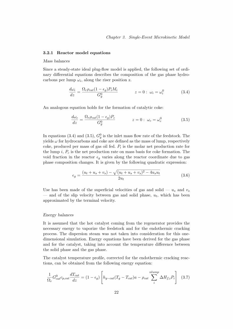
Chapter 3. Single-Event Microkinetic Model
3.2.1 Reactor model equations
Mass balances
Since a steady-state ideal plug-flow model is applied, the following set of ordi-nary differential equations describes the composition of the gas phase hydro-carbons per lump ωi, along the riser position z.
dωi
dz=
Ωrρcat(1− εg)PiMi
G0g
z = 0 : ωi = ω0i (3.4)
An analogous equation holds for the formation of catalytic coke:
dωc
dz=
Ωrρcat(1− εg)Pc
G0g
z = 0 : ωc = ω0c (3.5)
In equations (3.4) and (3.5), G0g is the inlet mass flow rate of the feedstock. The
yields ω for hydrocarbons and coke are defined as the mass of lump, respectivelycoke, produced per mass of gas oil fed. Pi is the molar net production rate forthe lump i, Pc is the net production rate on mass basis for coke formation. Thevoid fraction in the reactor εg varies along the reactor coordinate due to gasphase composition changes. It is given by the following quadratic expression:
εg =(ut + us + vs)−
√(ut + us + vs)2 − 4usut
2ut(3.6)
Use has been made of the superficial velocities of gas and solid — us and vs
— and of the slip velocity between gas and solid phase, ut, which has beenapproximated by the terminal velocity.
Energy balances
It is assumed that the hot catalyst coming from the regenerator provides thenecessary energy to vaporize the feedstock and for the endothermic crackingprocess. The dispersion steam was not taken into consideration for this one-dimensional simulation. Energy equations have been derived for the gas phaseand for the catalyst, taking into account the temperature difference betweenthe solid phase and the gas phase.
The catalyst temperature profile, corrected for the endothermic cracking reac-tions, can be obtained from the following energy equation:
1Ωr
G0catcp,cat
dTcat
dz= (1− εg)
[hg−cat(Tg − Tcat)a− ρcat
nlump∑i
∆Hf,iPi
](3.7)
22
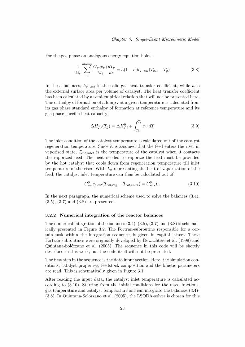
Chapter 3. Single-Event Microkinetic Model
For the gas phase an analogous energy equation holds:
1Ωr
nlump∑i
Gg,icp,i
Mi
dTg
dz= a(1− ε)hg−cat(Tcat − Tg) (3.8)
In these balances, hg−cat is the solid-gas heat transfer coefficient, while a isthe external surface area per volume of catalyst. The heat transfer coefficienthas been calculated by a semi-empirical relation that will not be presented here.The enthalpy of formation of a lump i at a given temperature is calculated fromits gas phase standard enthalpy of formation at reference temperature and itsgas phase specific heat capacity:
∆Hf,i(Tg) = ∆H0f,i +
∫ Tg
T0
cp,idT (3.9)
The inlet condition of the catalyst temperature is calculated out of the catalystregeneration temperature. Since it is assumed that the feed enters the riser invaporized state, Tcat,inlet is the temperature of the catalyst when it contactsthe vaporized feed. The heat needed to vaporize the feed must be providedby the hot catalyst that cools down from regeneration temperature till inlettemperature of the riser. With Lv representing the heat of vaporization of thefeed, the catalyst inlet temperature can thus be calculated out of:
G0catcp,cat(Tcat,reg − Tcat,inlet) = G0
gasLv (3.10)
In the next paragraph, the numerical scheme used to solve the balances (3.4),(3.5), (3.7) and (3.8) are presented.
3.2.2 Numerical integration of the reactor balances
The numerical integration of the balances (3.4), (3.5), (3.7) and (3.8) is schemat-ically presented in Figure 3.2. The Fortran-subroutine responsible for a cer-tain task within the integration sequence, is given in capital letters. TheseFortran-subroutines were originally developed by Dewachtere et al. (1999) andQuintana-Solorzano et al. (2005). The sequence in this code will be shortlydescribed in this work, but the code itself will not be presented.
The first step in the sequence is the data input section. Here, the simulation con-ditions, catalyst properties, feedstock composition and the kinetic parametersare read. This is schematically given in Figure 3.1.
After reading the input data, the catalyst inlet temperature is calculated ac-cording to (3.10). Starting from the initial conditions for the mass fractions,gas temperature and catalyst temperature one can integrate the balances (3.4)-(3.8). In Quintana-Solorzano et al. (2005), the LSODA-solver is chosen for this
23

Chapter 3. Single-Event Microkinetic Model
task. This solver has the ability to switch between stiff and nonstiff methods.The BDF scheme combined with variable step size and order control is usedfor the implicit integration. The iteration stops successfully once a prescribederror tolerance is reached or just stops after a maximum number of non-lineariteration steps. LSODA uses Adams predictor-corrector methods for nonstiffsystems (Hindmarsh, 1980).
During a solution loop of LSODA, several evaluations of the right-hand side ofthe balances are needed to estimate the Jacobian matrix (for stiff methods) orto calculate the new mass fractions directly in an explicit way. In these functionevaluations, the net production rate of each species has to be calculated. Theseproduction rates depend on the mass fraction of the lumps in the gas phaseand on the total carbenium ion concentration at a certain axial coordinate. Aspreviously mentioned, the carbenium ion concentration can be found by solvingits pseudo stationary state balance. The subroutine FCN3 expresses this balancein an algebraic non-linear equation with one unknown variable, Cb0 and thesubroutine DNSQE solves this equation for Cb0. Knowing the total carbeniumion concentration, all the reaction rates can be found.
The solution procedure stops when the axial coordinate has reached the lengthof the riser.
Figure 3.1: Required input information for performing the riser simulation
24

Chapter 3. Single-Event Microkinetic Model
Figure 3.2: Flow diagram of the one-dimensional riser simulation
25
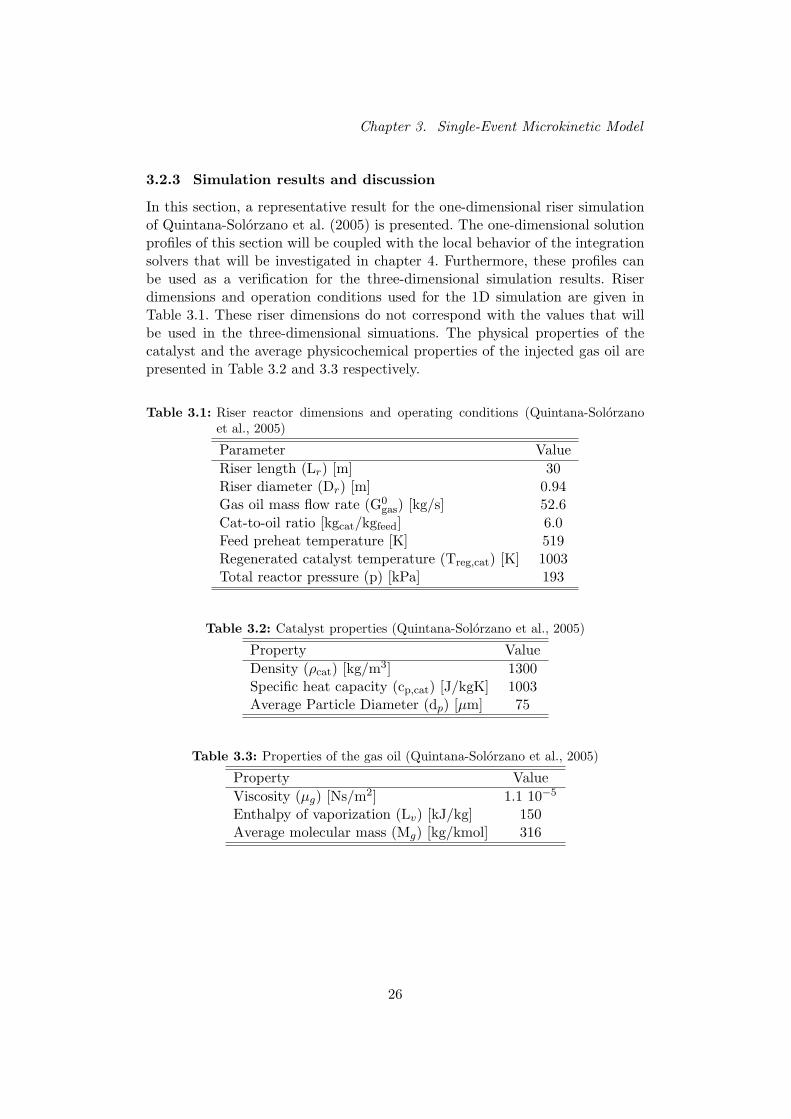
Chapter 3. Single-Event Microkinetic Model
3.2.3 Simulation results and discussion
In this section, a representative result for the one-dimensional riser simulationof Quintana-Solorzano et al. (2005) is presented. The one-dimensional solutionprofiles of this section will be coupled with the local behavior of the integrationsolvers that will be investigated in chapter 4. Furthermore, these profiles canbe used as a verification for the three-dimensional simulation results. Riserdimensions and operation conditions used for the 1D simulation are given inTable 3.1. These riser dimensions do not correspond with the values that willbe used in the three-dimensional simuations. The physical properties of thecatalyst and the average physicochemical properties of the injected gas oil arepresented in Table 3.2 and 3.3 respectively.
Table 3.1: Riser reactor dimensions and operating conditions (Quintana-Solorzanoet al., 2005)
Parameter ValueRiser length (Lr) [m] 30Riser diameter (Dr) [m] 0.94Gas oil mass flow rate (G0
gas) [kg/s] 52.6Cat-to-oil ratio [kgcat/kgfeed] 6.0Feed preheat temperature [K] 519Regenerated catalyst temperature (Treg,cat) [K] 1003Total reactor pressure (p) [kPa] 193
Table 3.2: Catalyst properties (Quintana-Solorzano et al., 2005)
Property ValueDensity (ρcat) [kg/m3] 1300Specific heat capacity (cp,cat) [J/kgK] 1003Average Particle Diameter (dp) [µm] 75
Table 3.3: Properties of the gas oil (Quintana-Solorzano et al., 2005)
Property ValueViscosity (µg) [Ns/m2] 1.1 10−5
Enthalpy of vaporization (Lv) [kJ/kg] 150Average molecular mass (Mg) [kg/kmol] 316
26

Chapter 3. Single-Event Microkinetic Model
Gas and catalyst temperature
The evolution of the catalyst and the gas phase temperature along the riserposition is presented in Figure 3.3. Using formula (3.10), the inlet catalyst tem-perature is 978 K. In the beginning part of the riser, the gas phase temperaturesharply increases at the expense of the catalyst temperature. After about 1.5meters, both temperature profiles overlap, exhibiting a smooth decrease towardsthe outlet due to endothermic cracking reactions.
Figure 3.3: Temperature of the catalyst and gas phase along the riser
Product evolution along the riser
Figure 3.4 illustrates the mass yields of the cracking products as a function of theriser axial position. During the first meters of the riser, the heavy hydrocarbonscontact the hot regenerated catalyst. The high catalyst temperature and thehigh HCO concentration cause high reactivity in the inlet section of the riser.The high reactivity results in vigorous cracking, yielding the formation of animportant amount of lighter hydrocarbons (in particular gasoline) and coke.About 60% of the coke observed at the riser outlet is formed in the first 2 metersof the riser. As the reactions proceed along the riser, cracking occurs to a lesserextent because the temperature of the solid drops, the catalyst deactivationincreases and the amount of light hydrocarbons — which are less susceptible tocracking — increases.
From 10 meters onwards, the HCO-conversion becomes very slow and the prod-uct distribution undergoes few changes. After ten meters, about 90 wt% of thegasoline leaving the riser has been formed, which reflects that the gasoline pre-cursors of the feedstock have been partially consumed. At the riser outlet, theoverall gas oil conversion corresponds to 65 wt% while gasoline and LPG yields
27
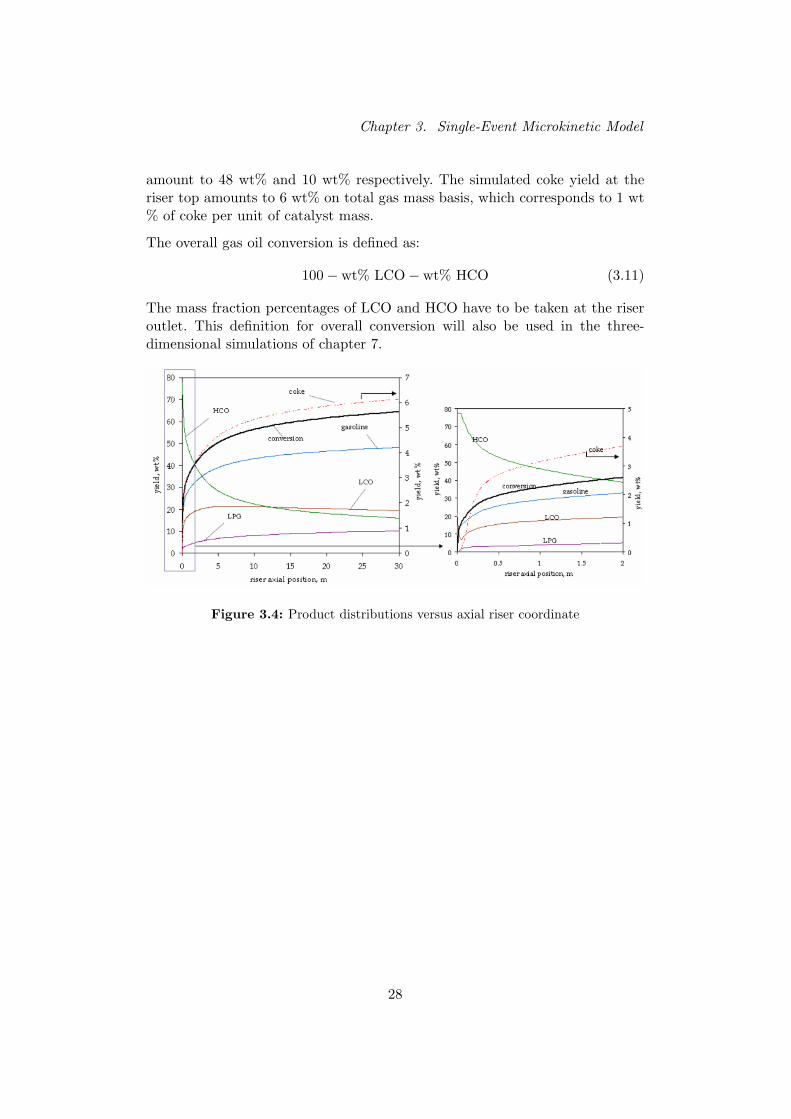
Chapter 3. Single-Event Microkinetic Model
amount to 48 wt% and 10 wt% respectively. The simulated coke yield at theriser top amounts to 6 wt% on total gas mass basis, which corresponds to 1 wt% of coke per unit of catalyst mass.
The overall gas oil conversion is defined as:
100− wt% LCO− wt% HCO (3.11)
The mass fraction percentages of LCO and HCO have to be taken at the riseroutlet. This definition for overall conversion will also be used in the three-dimensional simulations of chapter 7.
Figure 3.4: Product distributions versus axial riser coordinate
28

Chapter 4
Numerical analysis of the Single-Event MicroKineticModel
4.1 Introduction
In this chapter, a numerical analysis of the Single-Event MicroKinetic modelis presented. The model is represented by the one-dimensional reactor modelequations given in section 3.2.1. The goal of this analysis is to have an improvedinsight in the numerical integration behavior of the kinetic model. The conclu-sions of this analysis result in an estimate of the stiffness of the SEMK-modeland in the selection of a suitable solver. This solver is used for the integration ofthe three-dimensional transport equations of each component. Therefore, onlythe one-dimensional reactor balances for the 677 lumps and coke — equations(3.4)-(3.5) — are considered in the numerical analysis, as these balances con-tain the net production rates of each component. The numerical evaluation ofthe energy balances (3.7)-(3.8) does not give any additional information on thekinetic model.
4.2 Stability theory for a linear set of equations
4.2.1 Stability of the exact solution
Consider the following linear coupled set of equations:
dω
dz= Aω (4.1)
According to Lomax et al. (2003), the general solution of the set of equations(4.1) can be written as:
ω(z) =N+1∑m=1
cmeλmzxm + A−1b(z) (4.2)
29

Chapter 4. Numerical analysis of the Single-Event MicroKinetic Model
The first group of terms on the right-hand side of equation (4.2) is referredto as the homogeneous solution. It represents the transient part of the generalsolution. The second group is the particular solution, which corresponds phys-ically with the steady-state solution of (4.8). In the general solution (4.2), λm
is the mth eigenvalue of the Jacobian matrix A and xm is the correspondingeigenvector. The coefficients cm are determined in such a way that the initialconditions for the set of equations (4.1) are fulfilled.
The stability of the set of equations (4.1) depends entirely on the eigensystem.Per definition, the coupled system of ODEs (4.1) is inherently stable for aconstant coefficient matrix A if ω remains bounded for t → ∞, under thecondition that b is constant. Regarding general solution (4.2), this is thus trueif and only if <(λm) ≤ 0, ∀m. The expression <(λm) corresponds with the realpart of the mth eigenvalue.
4.2.2 Stability in numerical integration of linear set of equations
For the numerical integration of the set of equations (4.1), the one-dimensionalspace is divided in intervals. A numerical integration step implies that the valueof ω at coordinate z = zn+1 is determined starting from the value at z = zn.Using a fixed step length of h, the exact solution of the system at z = zn = nhbecomes:
ω(zn) =N+1∑m=1
cm(eλmh)nxm + A−1b(zn) (4.3)
The application of a numerical integration method thus corresponds with ap-proximating the exponential factors as σ = f(λh). The first order explicit Eu-ler method for example, uses a truncated expansion of the exponential factor:eλmh ≈ σ = 1 + λh. The numerical solution at z = zn then equals:
ωn =N+1∑m=1
cm(σm)nxm + A−1bn (4.4)
Clearly, an integration method — which is uniquely determined by the relationσ = f(λh) — is numerically stable if and only if |(σm)| ≤ 1, ∀m. The stabil-ity of a numerical method — this is a completely different concept than thestability of a set of equations — is thus determined by the eigenspectrum ofthe set of equations that has to be solved and by the integration step size. Foreach numerical integration technique, a given region in the complex λh planecorresponds with a stable integration. Stable and unstable regions are separatedby stability contours. An example of the stability contour of the second orderbackward implicit method is given in Figure 4.1. In this figure, R(λh) and I(λh)stand for respectively the real and imaginary part of λh. The stability conditionbecomes |σ| ≤ 1 with σ a solution of σ2(1− 2
3λh)− 43σ + 1
3 = 0 (Lomax et al.,
30

Chapter 4. Numerical analysis of the Single-Event MicroKinetic Model
2003). The stability region for this method contains the entire negative realplane.
Figure 4.1: Stability contour of the second order backward implicit method (BDF)
The above considerations demonstrate the importance of the selection of anappropriate integration method. If the step length h has to be excessively smallto force the eigenspectrum into the stable region (e.g. with the explicit Eulermethod (Lomax et al., 2003)), an integration method with a more extendedstability region has to be chosen in order to reduce the CPU time by usingincreased step sizes. Therefore, the eigenvalues of the SEMK-model will bedetermined and an appropriate integration method is selected using the SEMK-model’s stability region.
4.3 Determination of the eigenvalues of the SEMK-model
4.3.1 Linearization of the nonlinear SEMK-model
The one-dimensional reactor balances (3.4)-(3.5) can be represented by thefollowing general formulation:
dω
dz= B(ω) (4.5)
Here, ω is the (N + 1)-dimensional vector containing the mass fractions ofthe N lumps and coke. B is the (N + 1)-dimensional vector that representsthe right-hand side function in the balances (3.4)-(3.5). This nonlinear vectorfunction can be approximated according to a first order Taylor expansion abouta reference state at position zn:
B(ω) = B(ωn)+An(ω−ωn)+O[(ω−ωn)2] ≈ Anω+[B(ωn)−Anωn] (4.6)
A is the Jacobian matrix, which is defined by:
A = (ai,j) =∂Bi
∂ωj(4.7)
31
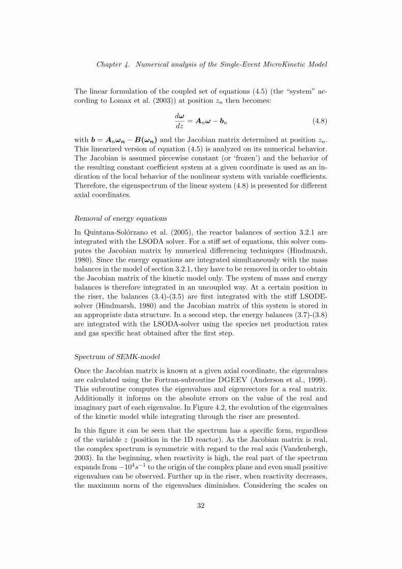
Chapter 4. Numerical analysis of the Single-Event MicroKinetic Model
The linear formulation of the coupled set of equations (4.5) (the “system” ac-cording to Lomax et al. (2003)) at position zn then becomes:
dω
dz= Anω − bn (4.8)
with b = Anωn −B(ωn) and the Jacobian matrix determined at position zn.This linearized version of equation (4.5) is analyzed on its numerical behavior.The Jacobian is assumed piecewise constant (or ‘frozen’) and the behavior ofthe resulting constant coefficient system at a given coordinate is used as an in-dication of the local behavior of the nonlinear system with variable coefficients.Therefore, the eigenspectrum of the linear system (4.8) is presented for differentaxial coordinates.
Removal of energy equations
In Quintana-Solorzano et al. (2005), the reactor balances of section 3.2.1 areintegrated with the LSODA solver. For a stiff set of equations, this solver com-putes the Jacobian matrix by numerical differencing techniques (Hindmarsh,1980). Since the energy equations are integrated simultaneously with the massbalances in the model of section 3.2.1, they have to be removed in order to obtainthe Jacobian matrix of the kinetic model only. The system of mass and energybalances is therefore integrated in an uncoupled way. At a certain position inthe riser, the balances (3.4)-(3.5) are first integrated with the stiff LSODE-solver (Hindmarsh, 1980) and the Jacobian matrix of this system is stored inan appropriate data structure. In a second step, the energy balances (3.7)-(3.8)are integrated with the LSODA-solver using the species net production ratesand gas specific heat obtained after the first step.
Spectrum of SEMK-model
Once the Jacobian matrix is known at a given axial coordinate, the eigenvaluesare calculated using the Fortran-subroutine DGEEV (Anderson et al., 1999).This subroutine computes the eigenvalues and eigenvectors for a real matrix.Additionally it informs on the absolute errors on the value of the real andimaginary part of each eigenvalue. In Figure 4.2, the evolution of the eigenvaluesof the kinetic model while integrating through the riser are presented.
In this figure it can be seen that the spectrum has a specific form, regardlessof the variable z (position in the 1D reactor). As the Jacobian matrix is real,the complex spectrum is symmetric with regard to the real axis (Vandenbergh,2003). In the beginning, when reactivity is high, the real part of the spectrumexpands from−104s−1 to the origin of the complex plane and even small positiveeigenvalues can be observed. Further up in the riser, when reactivity decreases,the maximum norm of the eigenvalues diminishes. Considering the scales on
32
Chapter 4. Numerical analysis of the Single-Event MicroKinetic Model
the axis, it is seen that the spectrum remains close to the real axis. Since theeigenvalues of the set of equations change as the position in the riser varies, theSEMK-model is clearly a nonlinear system. This is also seen in the evolution ofthe eigenvectors — corresponding each with a given eigenvalue — because theyvary even more significantly with the coordinate z. This nonlinear behavior isa consequence of the presence of species partial pressures in the numerator anddenominator of the carbenium ion concentration balance. Therefore the elemen-tary reaction rates do not have a first order dependence on the concentrationof the components of the model. The spectrum of the SEMK-model is thus dif-ferent from the spectrum of a set of rate equations for a network of first-orderreversible reactions. The eigenvalues of the latter network are situated on thenegative real axis (Wei and Prater, 1962).
-1300
-800
-300
200
700
1200
-10000 -8000 -6000 -4000 -2000 0
Real part [1/m]
Imag
inar
y pa
rt [
1/m
]
z = 0,054 mz = 0,1236 m z = 0,2028 m
Figure 4.2: Spectrum of frozen Jacobians at different reactor coordinates
In the next section, some general aspects concerning the stiffness of linear andnonlinear set of equations are discussed. They are helpful in selecting a suitableintegration method.
33

Chapter 4. Numerical analysis of the Single-Event MicroKinetic Model
4.4 Stiffness of nonlinear systems
Generally speaking, integration techniques can be divided in implicit and ex-plicit methods. Implicit methods have an enlarged stability region and theyare required if the problem has a large degree of stiffness. As a consequence,the degree of stiffness of the considered system is an important indication whenchoosing an integration method. The definition and determination of stiffness ishowever not trivial and certainly not uniform in literature. According to Lomaxet al. (2003), a linear constant coefficient system is stiff if all of its eigenvalueshave a negative real part and the stiffness ratio is large. This is a commonlyused definition of stiffness, in which the stiffness ratio is formulated as:
Cr =|λmax||λmin|
(4.9)
where |λmax| and |λmin| are respectively the largest and smallest modulus ofall the eigenvalues of the set of equations. In applying this definition to theSEMK-model, a few practical obstacles are perceived:• DGEEV-calculations indicate that some eigenvalues have a slightly pos-
itive real part. The above definition of stiffness ratio is not valid in thiscase.
• Even if the eigenvalues with positive real part are discarded for thecalculation of the stiffness ratio, DGEEV-calculations indicate that someeigenvalues are zero (remark that there is a certain absolute error). Verysmall eigenvalues (order 10−8s−1), with relative errors above 1 are alsofound. This means that the determination of eigenvalues close to zero isnot accurate. This could have a large influence on the stiffness ratio Cr
since the smallest eigenvalue is used as the denominator. The estimationof the stiffness by this ratio is therefore useless.
• Supposing that at least one of the zero-eigenvalues is correctly deter-mined, the eigenvalue with the smallest modulus is exact zero. Whateverthe value of the remaining eigenvalues might be, the stiffness ratio is nowinfinite regardless of the degree of real stiffness. The zero-eigenvalue doesnot necessarily introduce stiffness into the solution, because the contri-bution of that eigenvalue to the exact solution is a constant term.
Not only the above practical problems prevent applying the definition of Lomaxet al. (2003) to determine the stiffness. Other objections of a theoretical pointof view can be made. According to Lambert (1990), analyzing the behaviorof a nonlinear system by freezing the Jacobian gives no more than qualita-tive information on the stiffness and the evolution of the system. In Lambert(1990), several examples are given where the prediction of quantitative aspectsof nonlinear systems using the frozen Jacobian technique gives incorrect results.
Therefore, the more pragmatic definition of stiffness proposed by Lambert(1990) is applied in this work, as has been done by Cartwright and Piro (1992).This definition is related to what can be observed in practice:
34

Chapter 4. Numerical analysis of the Single-Event MicroKinetic Model
“If a numerical method with a finite region of absolute stabilityapplied to a system with any initial conditions, is forced to use ina certain interval of integration a step length which is excessivelysmall in relation to the smoothness of the exact solution in thisinterval, then the system is said to be stiff in that interval.”
The excessive smallness of a steplength depends on the stage reached in the inte-gration. When fast transients still occur, the exact solution is not at all smooth;a very small steplength is natural and should not be seen as ‘excessively small’.On the other hand, when the exact solution is smooth, a very small stepsize isnot natural. As a consequence of the practical character of this definition, it isstill valid when nonlinear systems or systems with positive eigenvalues (or evenzero-eigenvalues) are investigated. Therefore it is more suitable to be appliedto the SEMK-model.
In order to apply the definition of Lambert (1990), four different solvers areapplied to integrate the set of equations (3.4)-(3.5) and their corresponding in-tegration behavior is be analyzed. This information will then be used to decide,according to Lambert’s definition, whether the system is stiff or not and toselect the most appropriate integration method.
4.5 Selection of a suitable integration method
When performing a three-dimensional simulation with the SEMK-model, theintegration of the one-dimensional reactor balances (3.4)-(3.5) is executed oncefor each grid cell (see chapters 5 & 6). Consequently, it is very important tominimize the required CPU time for a one-dimensional integration. Therefore,a suitable integration method is chosen in this section. The solvers that areinvestigated are the LSODA solver, the LSODE Adams Bashford solver (AB),the LSODE backward differencing solver (BDF) and the stabilized Runge-Kuttasolver. The LSODE-BDF solver integrates implicitly (stiff), the LSODE-ABsolver integrates explicitly (non-stiff) and the LSODA solver switches betweenthese two approaches.
4.5.1 The stabilized Runge-Kutta solver
LSODA and LSODE (Hindmarsh, 1980) are well known solvers that can beused for many applications. For the application in this work, a more specificsolver is found in literature. Although reliable quantitative conclusions can notbe drawn from the evolution of the eigenvalue spectrum of frozen nonlinearsystems, such an analysis generally provides a good qualitative image of thedistribution of the eigenvalues. Therefore, it is assumed in this work that thespectrum of the SEMK-model can be used to search for more specific solvers.
35

Chapter 4. Numerical analysis of the Single-Event MicroKinetic Model
In integrating mildly stiff problems, standard explicit methods require smalltime steps to obtain a stable integration. Implicit methods on the other hand,require one or more algebraic system solutions at each integration step. Thisapproach can become costly in higher space dimensions. It can thus be usefulto apply a method that is in between these two extremes. In Hundsdorfer andVerwer (2003), a family of stabilized Runge-Kutta or Runge-Kutta-Chebyshev(RKC) solvers is presented. These methods are explicit and possess an extendedreal stability region with a length proportional to m2, with m the number ofstages. An example of the stability region of a five stage second-order RKC isgiven in Figure 4.3. These stabilized methods are appropriate for the solution ofmildly stiff problems with eigenvalues that are close to the negative real axis. Itcould thus be advantageous to use such methods for the SEMK-model becauseits eigenvalues are extended over a large range of the negative complex plane,but close to the real axis at the same time.
Figure 4.3: Stability region of a five stage second-order RKC
In the next section, the RKC-code of Sommeijer et al. (1998) is used to integratethe one-dimensional reactor balances. The program uses an estimate of thespectral radius of the system in each step to select the minimal number ofstages m resulting in a stable integration. Once the required number of stages isknown, the corresponding member of the stabilized Runge-Kutta family is usedto perform the integration. Sommeijer et al. (1998) state that other methodsshould be considered if the number of stages exceeds 100, because the systemis then more than mildly stiff.
36
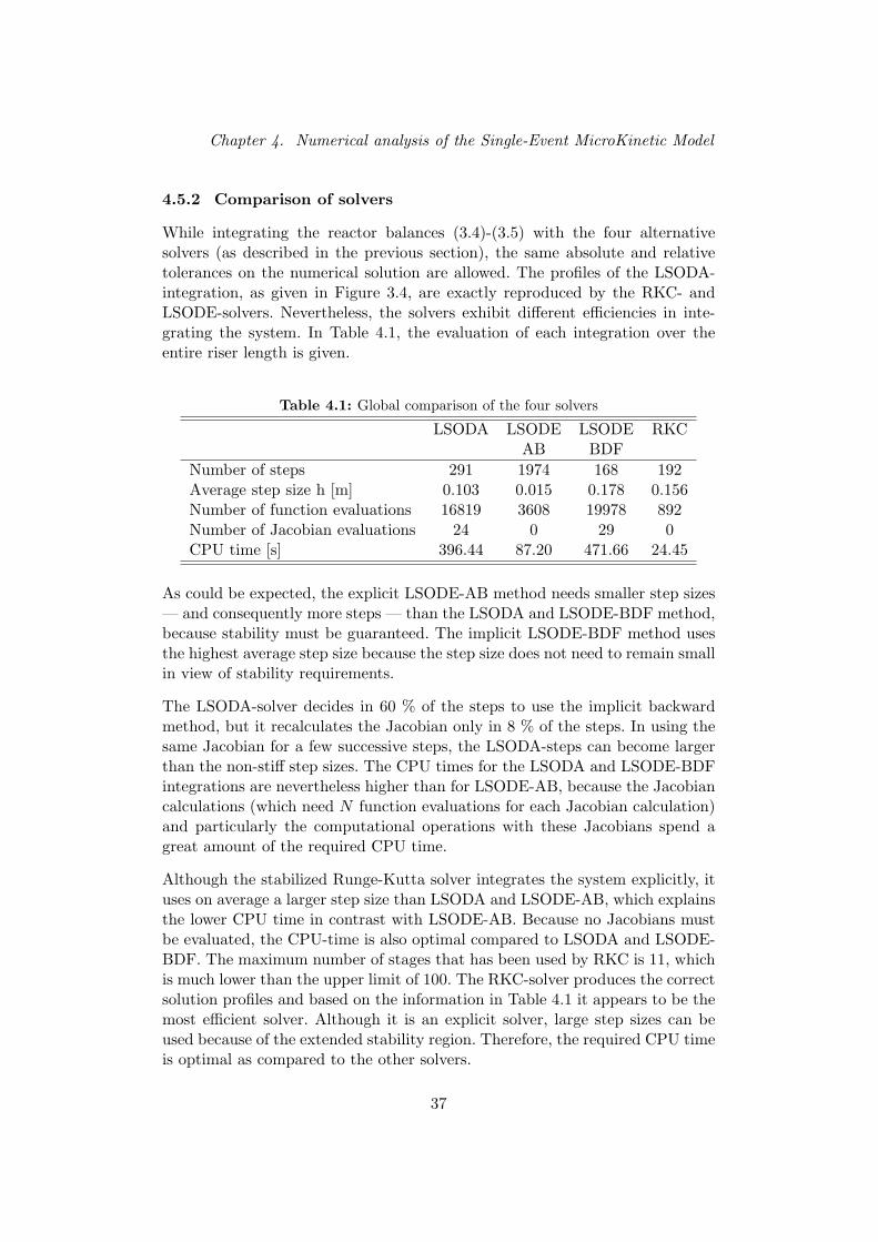
Chapter 4. Numerical analysis of the Single-Event MicroKinetic Model
4.5.2 Comparison of solvers
While integrating the reactor balances (3.4)-(3.5) with the four alternativesolvers (as described in the previous section), the same absolute and relativetolerances on the numerical solution are allowed. The profiles of the LSODA-integration, as given in Figure 3.4, are exactly reproduced by the RKC- andLSODE-solvers. Nevertheless, the solvers exhibit different efficiencies in inte-grating the system. In Table 4.1, the evaluation of each integration over theentire riser length is given.
Table 4.1: Global comparison of the four solvers
LSODA LSODE LSODE RKCAB BDF
Number of steps 291 1974 168 192Average step size h [m] 0.103 0.015 0.178 0.156Number of function evaluations 16819 3608 19978 892Number of Jacobian evaluations 24 0 29 0CPU time [s] 396.44 87.20 471.66 24.45
As could be expected, the explicit LSODE-AB method needs smaller step sizes— and consequently more steps — than the LSODA and LSODE-BDF method,because stability must be guaranteed. The implicit LSODE-BDF method usesthe highest average step size because the step size does not need to remain smallin view of stability requirements.
The LSODA-solver decides in 60 % of the steps to use the implicit backwardmethod, but it recalculates the Jacobian only in 8 % of the steps. In using thesame Jacobian for a few successive steps, the LSODA-steps can become largerthan the non-stiff step sizes. The CPU times for the LSODA and LSODE-BDFintegrations are nevertheless higher than for LSODE-AB, because the Jacobiancalculations (which need N function evaluations for each Jacobian calculation)and particularly the computational operations with these Jacobians spend agreat amount of the required CPU time.
Although the stabilized Runge-Kutta solver integrates the system explicitly, ituses on average a larger step size than LSODA and LSODE-AB, which explainsthe lower CPU time in contrast with LSODE-AB. Because no Jacobians mustbe evaluated, the CPU-time is also optimal compared to LSODA and LSODE-BDF. The maximum number of stages that has been used by RKC is 11, whichis much lower than the upper limit of 100. The RKC-solver produces the correctsolution profiles and based on the information in Table 4.1 it appears to be themost efficient solver. Although it is an explicit solver, large step sizes can beused because of the extended stability region. Therefore, the required CPU timeis optimal as compared to the other solvers.
37
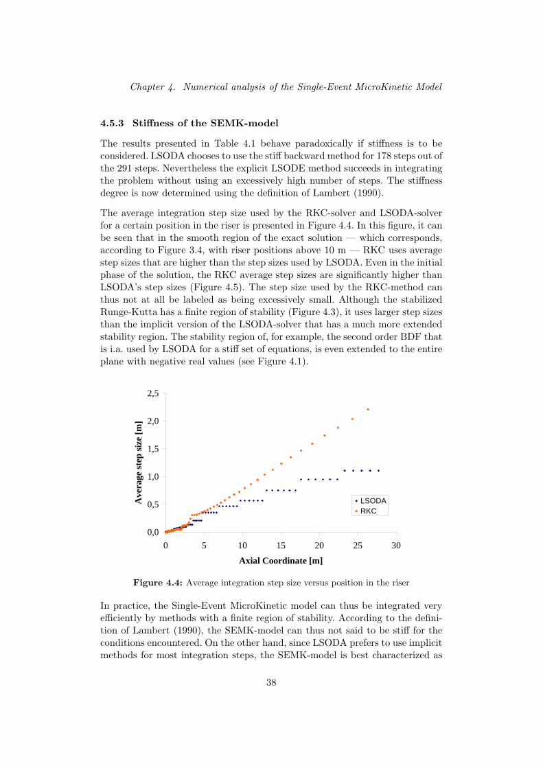
Chapter 4. Numerical analysis of the Single-Event MicroKinetic Model
4.5.3 Stiffness of the SEMK-model
The results presented in Table 4.1 behave paradoxically if stiffness is to beconsidered. LSODA chooses to use the stiff backward method for 178 steps out ofthe 291 steps. Nevertheless the explicit LSODE method succeeds in integratingthe problem without using an excessively high number of steps. The stiffnessdegree is now determined using the definition of Lambert (1990).
The average integration step size used by the RKC-solver and LSODA-solverfor a certain position in the riser is presented in Figure 4.4. In this figure, it canbe seen that in the smooth region of the exact solution — which corresponds,according to Figure 3.4, with riser positions above 10 m — RKC uses averagestep sizes that are higher than the step sizes used by LSODA. Even in the initialphase of the solution, the RKC average step sizes are significantly higher thanLSODA’s step sizes (Figure 4.5). The step size used by the RKC-method canthus not at all be labeled as being excessively small. Although the stabilizedRunge-Kutta has a finite region of stability (Figure 4.3), it uses larger step sizesthan the implicit version of the LSODA-solver that has a much more extendedstability region. The stability region of, for example, the second order BDF thatis i.a. used by LSODA for a stiff set of equations, is even extended to the entireplane with negative real values (see Figure 4.1).
0,0
0,5
1,0
1,5
2,0
2,5
0 5 10 15 20 25 30
Axial Coordinate [m]
Ave
rage
ste
p si
ze [
m]
LSODARKC
Figure 4.4: Average integration step size versus position in the riser
In practice, the Single-Event MicroKinetic model can thus be integrated veryefficiently by methods with a finite region of stability. According to the defini-tion of Lambert (1990), the SEMK-model can thus not said to be stiff for theconditions encountered. On the other hand, since LSODA prefers to use implicitmethods for most integration steps, the SEMK-model is best characterized as
38

Chapter 4. Numerical analysis of the Single-Event MicroKinetic Model
a mildly stiff system for the conditions encountered. This corresponds to thetype of systems that the RKC-solver was designed for.
0,0E+00
2,0E-04
4,0E-04
6,0E-04
8,0E-04
1,0E-03
1,2E-03
1,4E-03
1,6E-03
1,8E-03
2,0E-03
0 0,02 0,04 0,06 0,08 0,1
Axial Coordinate [m]
Ave
rage
ste
p si
ze [
m]
RKCLSODA
Figure 4.5: Average integration step size in the initial phase
4.6 Conclusion
Based on the integration information of Table 4.1, the RKC-solver appears tobe the most efficient solver for the integration of the one-dimensional reactorbalances (3.4)-(3.5), with the conditions as described in chapter 3. As will beshown in chapter 6, the reaction integration of the three-dimensional continuitybalances for each component has mathematically the same form as the system(3.4)-(3.5) and therefore the RKC-solver will be applied for this integration aswell.
39
Chapter 5
Hydrodynamic model for reactive gas-solid flow
The model equations which describe a reactive multicomponent gas flow ac-companied by a solid particle stream, are presented in this chapter. First, somegeneral assumptions and considerations are made. Next, an introduction withrespect to the solution technique will be given and a global overview of the se-quence in solving the equations will be presented. Finally, the model equationsfor the two phases will be presented, including auxiliary relations concerningthe solid phase model.
5.1 General considerations and assumptions
In this section, the assumptions that have been made in order to perform thesimulations are presented.
• A three-dimensional simulation will be performed since, as will be shownin chapter 7, the catalyst inlet lies in a plane perpendicular to the gasoil feed nozzles. This gives rise to complex three-dimensional inlet con-ditions, which require a three-dimensional approach.
• A two phase, gas-solid model will be used. As in the one-dimensionalmodel of Quintana-Solorzano, it is assumed that instantaneous vapor-ization of the feed occurs at the bottom of the riser. In this way, thereis no need for a vaporization model.
• Only the riser section of the catalytic cracker will be simulated. Further-more, the riser will be assumed adiabatic which corresponds to realisticconditions. No external forces beside the gravitational force act on theriser volume.
• Since the catalyst particles consist of porous material, concentrationgradients of the reactive gas phase arise inside the pores. In spite ofthis reduced concentration at the inside catalyst surface, bulk gas phaseconcentrations will be introduced in the expressions for the reactionrates of this model. The model in this work does not account for theintraparticle gradients.
40

Chapter 5. Hydrodynamic model for reactive gas-solid flow
• The high particle mass loading in the riser section does not allow totrack the particles through the calculated flow field, i.e. Euler-Lagrangeapproach. The Euler-Euler approach will thus be applied, which impliesthat both phases are treated mathematically as interpenetrating con-tinua. The volume fraction of the phases is then a continuous functionof space and time and their sum is equal to one. With this approachseveral multiphase models exist. For fluidized beds it is recommendedto use the Eulerian granular flow model (Benyahia et al., 2003). Thisis the most complex and the most accurate model for gas-solid flow,because it solves continuity, momentum and energy balances for eachphase. Coupling is achieved through the pressure and interphase ex-change coefficients and constitutive laws for the solid phase are derivedfrom the kinetic theory of granular flow.
• Compressibility effects are encountered in gas flows at high velocityand/or in which there are large pressure variations. When the flow ve-locity approaches or exceeds the speed of sound of the gas or when thepressure change in the system is large, the variation of the gas densitywith pressure has a significant impact on the flow velocity, pressure, andtemperature. Incompressible flow will be assumed in this work, becausepressure variations and mach numbers remain small (see chapter 7). Thismeans that the gas phase density will be defined by the incompressibleideal gas law.
• The only net mass transfer between the two phases consists of cokedeposition on the catalyst particles. The deposition of coke will be mod-eled in the continuity equations of both phases, but the momentum andenergy tranfer as a consequence of this mass transfer will be neglected.
• Changes in composition of a component are a combination of three dif-ferent physical phenomena, i.e. convection, diffusion and reaction. Inthis work, the diffusion due to concentration gradients of the compo-nents will not be considered.
• The specific heat, viscosity and thermal conductivity of the gas phasewill be assumed independent of the gas phase composition. The com-position dependence of the viscosity and thermal conductivity has notbeen implemented because the individual data for each component wasnot directly available. The specific heat does change during reaction; thereason for assuming it constant will be given in section 5.3.5.
5.2 Solution sequence
In this work, the model equations are partially solved by the commercial sim-ulation package Fluent and partially by a user defined program, that interactswith Fluent. Fluent is not able to solve mass balances for more than 50 species.As the number of species in the single-event kinetic model equals 678 (see
41

Chapter 5. Hydrodynamic model for reactive gas-solid flow
chapter 3), a user-defined treatment of the component continuity equations isneeded. The use of the Eulerian multiphase model in Fluent prevents the useof a coupled solver that treats all the model equations simultaneously. More-over, coupled solvers are recommended for strongly compressible flows and theircomputational complexity is not needed for the simulations in this work. Hencethe segregated solution method, in which the governing equations are solvedsequentially, is applied. Because of the non-linear and coupled character of theequations, several iterations of the solution loop must be performed before aconverged solution is obtained.
Each iteration consists of the steps illustrated in Figure 5.1 and outlined below:
1. Fluid properties are updated, based on the current solution variables.2. The u-, v- and w-momentum equations are solved for each phase using
the current values for pressure and the updated properties.3. Since the velocities obtained in Step 2 may not satisfy the mass conser-
vation locally, a ‘Poisson-type’ equation pressure correction is derivedfrom the continuity equation. Solving this pressure correction equationresults in updated pressures, velocity fields and mass fluxes satisfyingthe continuity equations.
4. Temperatures of both phases are recalculated by solving the energyequation.
5. Equations, which take into account the turbulence of the mixture, aresolved.
6. Changes in composition of the fluid phase are determined by solving thedifferent mass balances for the components in the fluid mixture.
7. Convergence of the set of equations is checked.
These steps are repeated until convergence is reached.
The steps, outlined above, will be divided in two separate parts. In the firstpart, all the balances concerning the two global phases are considered. Thus, theconservation of mass, momentum, energy and the turbulence balances of eachphase, which can be solved using the corresponding properties of each phase,are separated from the other equations. These balances on the global fluid andsolid phase are solved by Fluent. In the second part, the balances concerningthe reactants and products involved in fluid catalytic cracking, are integratedby a user-defined program that interacts with Fluent. The composition of thefluid determines the global properties of the fluid phase: molar mass, density,viscosity, thermal conductivity and specific heat. The concept applied in thiswork thus consists of two steps:
1. Using the current properties, the balances for the fluid mixture and thesolid phase are solved. Considering the enumeration used above, thiscorresponds with steps 2, 3, 4 and 5. As a result, the velocity, pressureand temperature fields in the riser are obtained.
42
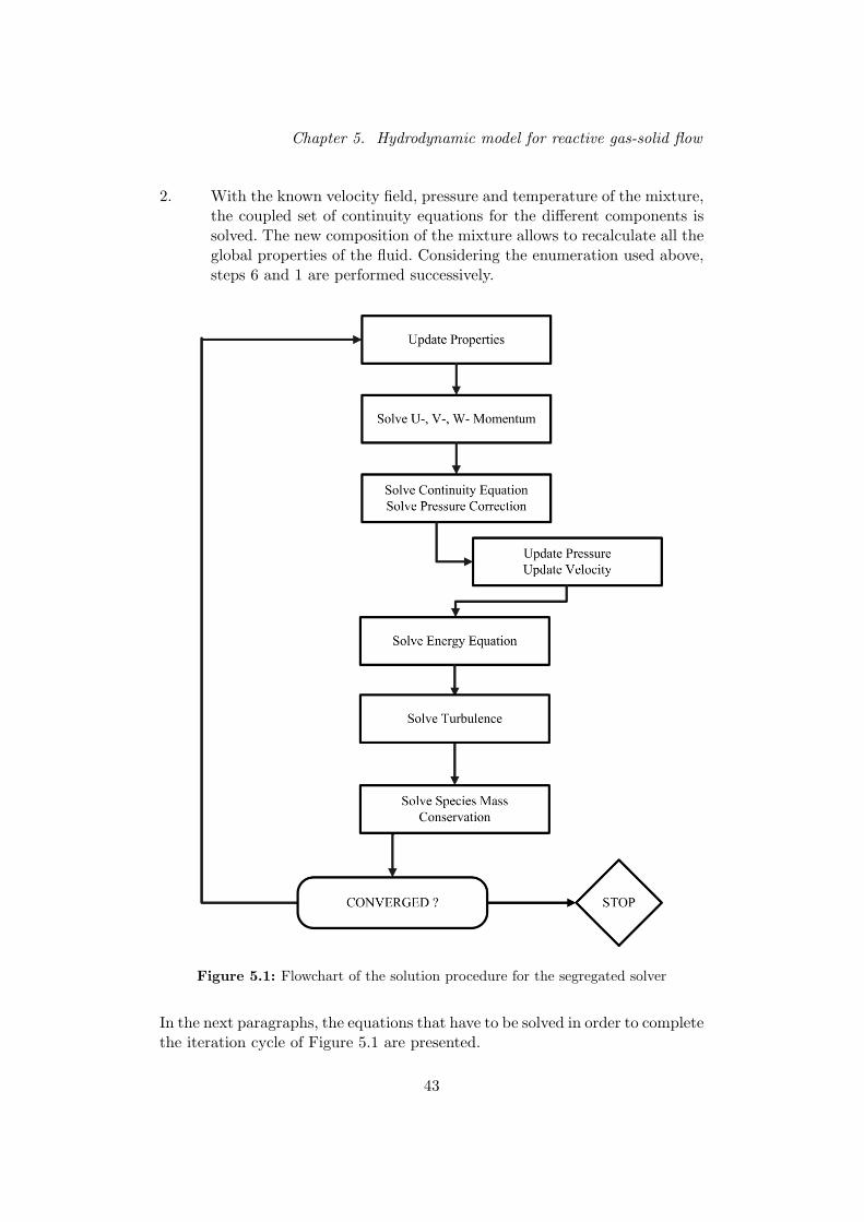
Chapter 5. Hydrodynamic model for reactive gas-solid flow
2. With the known velocity field, pressure and temperature of the mixture,the coupled set of continuity equations for the different components issolved. The new composition of the mixture allows to recalculate all theglobal properties of the fluid. Considering the enumeration used above,steps 6 and 1 are performed successively.
Figure 5.1: Flowchart of the solution procedure for the segregated solver
In the next paragraphs, the equations that have to be solved in order to completethe iteration cycle of Figure 5.1 are presented.
43

Chapter 5. Hydrodynamic model for reactive gas-solid flow
5.3 Model equations
As described in section 5.1, a three-dimensional, two-phase flow model is used.The balances for each phase will be presented, followed by the constitutive lawsconcerning the solid phase model. Next, the turbulence equations are treated.The concluding part of this section consists of the continuity equations for thecomponents and related constitutive laws for the fluid mixture properties. Asummary of all the model and auxiliary equations needed for the simulation ofa two phase gas-solid reactive mixture is given in Appendix A.
5.3.1 Balances on the fluid mixture and the solid phase
The conservation equations have to be derived for each phase. There are twogeneral continuity equations, two momentum equations and two energy bal-ances. Since these equations will be solved in a two-phase Fluent simulation,they are based on the equations presented in the Fluent user guide (2006).
Conservation of mass
The conservation of mass equations for the two phases express that the changein mass of each phase in a control volume (i.e. the grid cell) during time (theaccumulation term) is a result of a net convection of mass and mass transferbetween the two phases.
The equation for the gas phase is given by
∂
∂t(εgρg) +∇ · (εgρgu) = −mgs (5.1)
and for the solid phase by
∂
∂t(εsρs) +∇ · (εsρsv) = mgs (5.2)
For catalytic cracking, the mass transfer between the gas and solid phase onlyconsists of coke deposition on the catalyst. The term mgs thus equals the netmass of coke produced per mass catalyst and per unit of time, Pc, multipliedwith the catalyst fraction and the catalyst density. This term is formed bysolving the separate mass balance for coke and will be discussed in more detailin section 5.3.6. Note that the term mgs is not available in the standard Fluentmultiphase model, but it was computed by means of an external subroutine.
The mass balances for gas and solid phase are connected by the following rela-tion:
εs + εg = 1 (5.3)
44
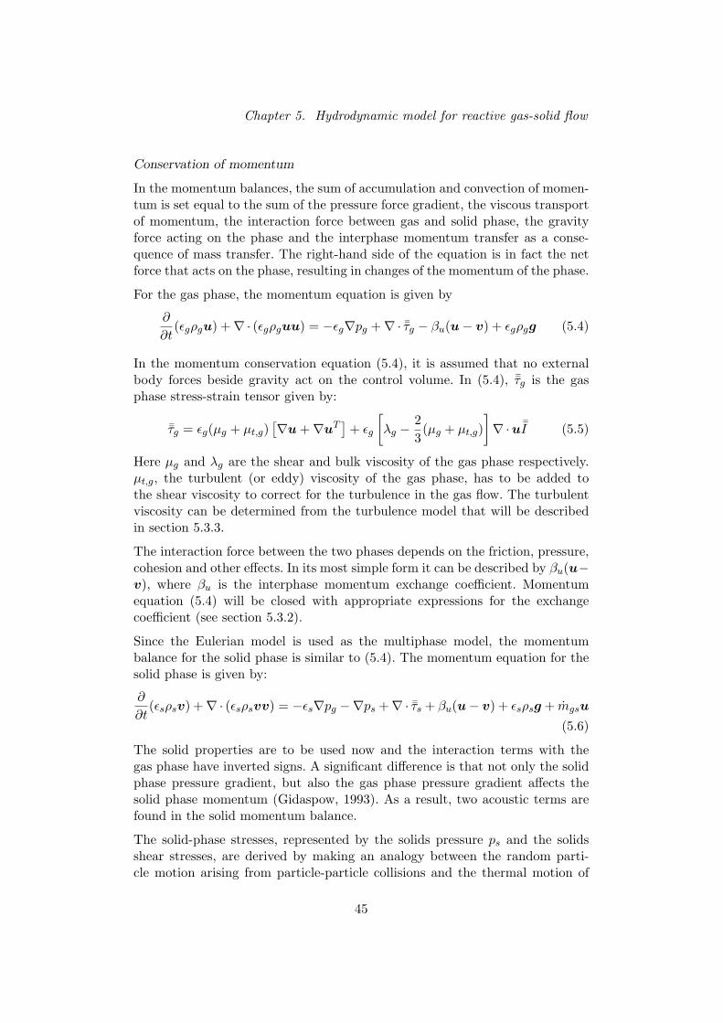
Chapter 5. Hydrodynamic model for reactive gas-solid flow
Conservation of momentum
In the momentum balances, the sum of accumulation and convection of momen-tum is set equal to the sum of the pressure force gradient, the viscous transportof momentum, the interaction force between gas and solid phase, the gravityforce acting on the phase and the interphase momentum transfer as a conse-quence of mass transfer. The right-hand side of the equation is in fact the netforce that acts on the phase, resulting in changes of the momentum of the phase.
For the gas phase, the momentum equation is given by
∂
∂t(εgρgu) +∇ · (εgρguu) = −εg∇pg +∇ · ¯τg − βu(u− v) + εgρgg (5.4)
In the momentum conservation equation (5.4), it is assumed that no externalbody forces beside gravity act on the control volume. In (5.4), ¯τg is the gasphase stress-strain tensor given by:
¯τg = εg(µg + µt,g)[∇u +∇uT
]+ εg
[λg −
23(µg + µt,g)
]∇ ·u ¯I (5.5)
Here µg and λg are the shear and bulk viscosity of the gas phase respectively.µt,g, the turbulent (or eddy) viscosity of the gas phase, has to be added tothe shear viscosity to correct for the turbulence in the gas flow. The turbulentviscosity can be determined from the turbulence model that will be describedin section 5.3.3.
The interaction force between the two phases depends on the friction, pressure,cohesion and other effects. In its most simple form it can be described by βu(u−v), where βu is the interphase momentum exchange coefficient. Momentumequation (5.4) will be closed with appropriate expressions for the exchangecoefficient (see section 5.3.2).
Since the Eulerian model is used as the multiphase model, the momentumbalance for the solid phase is similar to (5.4). The momentum equation for thesolid phase is given by:
∂
∂t(εsρsv) +∇ · (εsρsvv) = −εs∇pg −∇ps +∇ · ¯τs + βu(u− v) + εsρsg + mgsu
(5.6)
The solid properties are to be used now and the interaction terms with thegas phase have inverted signs. A significant difference is that not only the solidphase pressure gradient, but also the gas phase pressure gradient affects thesolid phase momentum (Gidaspow, 1993). As a result, two acoustic terms arefound in the solid momentum balance.
The solid-phase stresses, represented by the solids pressure ps and the solidsshear stresses, are derived by making an analogy between the random parti-cle motion arising from particle-particle collisions and the thermal motion of
45

Chapter 5. Hydrodynamic model for reactive gas-solid flow
molecules in a gas, taking into account the inelasticity of the granular phase.The solids pressure will be described in more detail in section 5.3.2. The solidstress-strain tensor is given by
¯τs = εs(µs + µt,s)[∇v +∇vT
]+ εs
[λs −
23(µs + µt,s)
]∇ ·v ¯I, (5.7)
which is analogous to the gas phase tensor (5.5).
The lift force and the virtual mass force have not been implemented in thismodel. The lift force on the catalyst particles is insignificant compared to thedrag force (βu(u − v)), so there is no reason to include this extra term. The‘virtual mass effect’ occurs when the secondary phase accelerates relative tothe primary phase. The inertia of the primary phase mass encountered by theaccelerating particles exerts a virtual mass force on the particles. This forceis significant only when the secondary phase density is much smaller than theprimary phase density, which is not the case here.
Conservation of energy
To describe the conservation of energy in Eulerian multiphase applications, aseparate enthalpy equation must be written for each phase. For the gas phase:
∂
∂t(εgρgEg)+∇ · (εgρguHg) = ∇ · (¯τg ·u)−∇ · (−εgkg∇Tg)
− βT (Tg − Ts) + εgρgg ·u + mgshgs
(5.8)
The change of total energy, expressed by accumulation and convection, is equalto the sum of the work done by the gas phase shear stress, the diffusive heattransport, the interphase heat transfer, the work performed by the gravitationalforce and the interphase energy transfer as a consequence of mass transfer ofcoke. In this energy balance, Hg represents the specific total enthalpy of thegas phase, which is the sum of the internal enthalpy of the gas phase hg and itskinetic energy:
Hg = hg +12u ·u (5.9)
The specific total energy of the gas phase Eg is in turn the sum of the internalenergy eg and the kinetic energy and is related to the specific total enthalpy as:
Eg = eg +12u ·u = Hg −
pg
ρg(5.10)
The term βT (Tg−Ts) is the intensity of heat exchange between the gas and solidphase. This term will be further discussed in section 5.3.2. The enthalpy hgs isthe specific enthalpy of the coke and represents the energy transfer accompanied
46

Chapter 5. Hydrodynamic model for reactive gas-solid flow
with the coke transfer. As pointed out in section 5.1, this enthalpy transfer issmall enough to be neglected.
A similar equation exists for the solid phase, but in this case the total energyEs, respectively enthalpy Hs is given by the sum of internal energy — respec-tively enthalpy — the kinetic energy v ·v and an extra term including the solidgranular temperature θs, which will be discussed in more detail in section 5.3.2.
Hs = hs +32θ +
12v ·v (5.11)
Es = es +32θ +
12v ·v (5.12)
The interphase convective heat transfer term is the opposite of the one in thegas phase energy equation, as all heat that leaves the gas phase enters the solidphase and vice versa. The solid momentum equation finally becomes:
∂
∂t(εsρsEs) +∇ · (εsρsvHs) = ∇ · (¯τs ·v)−∇ · (−εsks∇Ts)
+ βT (Tg − Ts) + εsρsg ·v − mgshgs + Ss
(5.13)
The energy equation for the solid phase has an extra energy source term Ss. Thiscontribution expresses the change in total enthalpy of the solid phase due tochemical reactions. Catalytic cracking is an endothermal process and since thecracking occurs on the solid particles, the temperature of the catalyst has to becorrected for these reactions. As a remark, it should be added that the enthalpychange of a medium due to reaction is normally embedded in the inward andoutward enthalpy fluxes of a control volume. These fluxes change due to thecomposition changes in the reacting medium. Here, reaction occurs only on thesolid phase. Since the composition of the solid phase does not change as a resultof these reactions, the temperature drop of the catalyst must be predicted bya source term. As the catalyst exchanges heat with the gas phase, the catalysttemperature drop is accompanied by a diminishing gas temperature. The exactformulation of this source term is handled in section 5.3.5.
The conservation laws for mass, momentum and energy together with relation(5.3) are used to solve for the primitive variables εg, εs, u, v, Tg, Ts and pg.The parameters which close the equations are µt, ps, βu, βT and µs. In the nextsections, it will be discussed how the latter parameters are determined.
5.3.2 Solid phase properties: the Kinetic Theory of Granular Flow
In this section, correlations for the unknown variables in the Eulerian multiphasemodel and the interaction between gas and solid phase are presented.
47
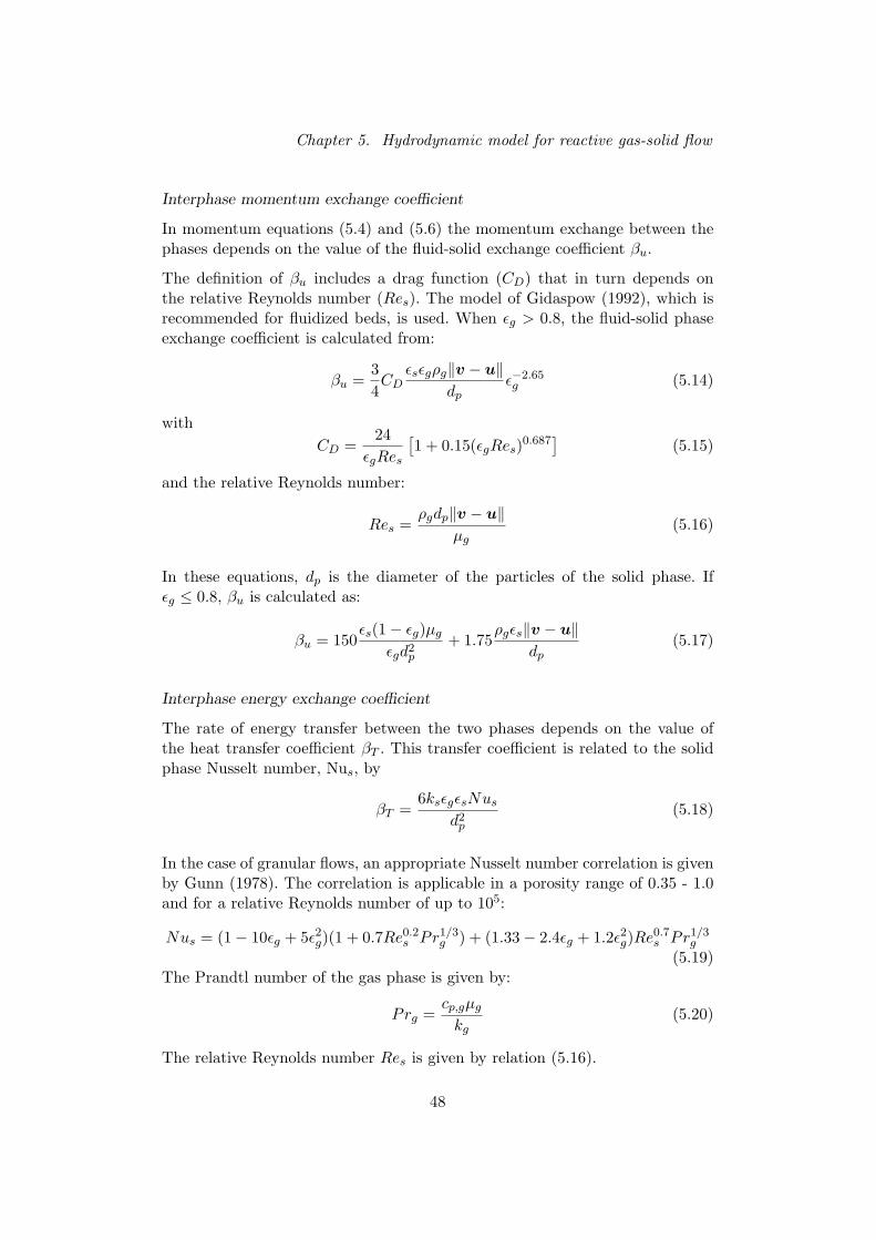
Chapter 5. Hydrodynamic model for reactive gas-solid flow
Interphase momentum exchange coefficient
In momentum equations (5.4) and (5.6) the momentum exchange between thephases depends on the value of the fluid-solid exchange coefficient βu.
The definition of βu includes a drag function (CD) that in turn depends onthe relative Reynolds number (Res). The model of Gidaspow (1992), which isrecommended for fluidized beds, is used. When εg > 0.8, the fluid-solid phaseexchange coefficient is calculated from:
βu =34CD
εsεgρg‖v − u‖dp
ε−2.65g (5.14)
withCD =
24εgRes
[1 + 0.15(εgRes)0.687
](5.15)
and the relative Reynolds number:
Res =ρgdp‖v − u‖
µg(5.16)
In these equations, dp is the diameter of the particles of the solid phase. Ifεg ≤ 0.8, βu is calculated as:
βu = 150εs(1− εg)µg
εgd2p
+ 1.75ρgεs‖v − u‖
dp(5.17)
Interphase energy exchange coefficient
The rate of energy transfer between the two phases depends on the value ofthe heat transfer coefficient βT . This transfer coefficient is related to the solidphase Nusselt number, Nus, by
βT =6ksεgεsNus
d2p
(5.18)
In the case of granular flows, an appropriate Nusselt number correlation is givenby Gunn (1978). The correlation is applicable in a porosity range of 0.35 - 1.0and for a relative Reynolds number of up to 105:
Nus = (1− 10εg + 5ε2g)(1 + 0.7Re0.2s Pr1/3
g ) + (1.33− 2.4εg + 1.2ε2g)Re0.7s Pr1/3
g
(5.19)The Prandtl number of the gas phase is given by:
Prg =cp,gµg
kg(5.20)
The relative Reynolds number Res is given by relation (5.16).
48

Chapter 5. Hydrodynamic model for reactive gas-solid flow
Solids pressure
Similar to the gas phase, the intensity of the particle velocity fluctuations de-termines the pressure of the solid phase. The kinetic energy associated withthe particle velocity fluctuations is represented by a pseudothermal or granulartemperature which is proportional to the mean square of the random motion ofthe particles. The solids pressure is composed of a kinetic term and a particlecollisions term (Lun et al., 1984):
ps = εsρsθs + 2ρs(1 + ess)ε2sg0θs (5.21)
where ess is the coefficient of restitution for particle collisions and θs is thegranular temperature, which will be described in the next section.
The function g0 is a distribution function that governs the transition from thecompressible condition with εs < εs,max — where the spacing between the solidparticles can still decrease — to the incompressible condition with εs = εs,max,where no further decrease in the spacing is possible. It is a correction factor thatmodifies the probability of collisions between grains when the solid granularphase becomes dense. In this work the empirical function of Lun et al. (1984)is used:
g0 =
[1−
(εs
εs,max
)1/3]−1
(5.22)
For a dilute solid phase (εs → 0), g0 tends to 1; in the limit when the solid phaseis extremely dense, the distribution function tends to infinity and consequentlyresults in a large solids pressure.
For the coefficient of restitution and the maximum packing limit, appropriateconstant values have to be chosen.
Granular Temperature
The granular temperature for the solid phase is proportional to the randommotion of the particles. The transport equation for the granular temperaturederived from the Kinetic Theory of Granular Flow takes the form (Ding andGidaspow, 1990):
32
[∂
∂t(ρsεsθs) +∇ · (ρsεsvθs)
]= ∇ ·
[(−ps
¯I + ¯τs) ·v]+∇ · (kθs∇θs)−γθs +φgs
(5.23)
In the right-hand side of this general equation, the contributions are: energycreation by the solid stress tensor, diffusion of solid phase energy, the collisionaldissipation of energy and the energy exchange between solid and fluid phaserespectively. In this work, the algebraic formulation of equation (5.23) will be
49
Chapter 5. Hydrodynamic model for reactive gas-solid flow
used. The latter is obtained by neglecting the time dependency, the convectionand the diffusion of energy in the transport equation.
The collisional dissipation of energy, γθs , is the rate of energy dissipation withinthe solid phase due to collisions between particles. In this work the correlationof Lun et al. (1984) is used:
γθs =12(1− e2
ss)g0
ds√
πρsε
2sθ
3/2s (5.24)
The transfer of the kinetic energy of random fluctuations in particle velocityfrom the solid phase to the fluid is represented by φgs and obtained as follows(Gidaspow et al., 1992):
φgs = −3βT θs (5.25)
Solids shear stresses
The solids stress tensor contains shear and bulk viscosities arising from particlemomentum exchange due to translation and collision. Neglecting the frictionalpart in the shear viscosity, the collisional and kinetic part are added to give:
µs = µs,col + µs,kin (5.26)
According to Gidaspow et al. (1992), the collisional granular viscosity is modeledas:
µs,col =45εsρsdpg0(1 + ess)
(θs
π
)1/2
(5.27)
The kinetic part is also calculated from Gidaspow et al. (1992):
µs,kin =10dpρs
√θsπ
96εs(1− ess)g0
[1 +
45g0εs(1 + ess)
]2
(5.28)
The solids bulk viscosity accounts for the resistance of the granular particles tocompression and expansion. Lun et al. (1984) propose:
λs =43εsρsdpg0(1 + ess)
(θs
π
)1/2
(5.29)
5.3.3 Turbulence modeling
A k-ε model is used for turbulence modeling in this work. This is the most simpleand efficient turbulence model that is able to predict accurately turbulence ofpractical engineering flow calculations. Launder and Spalding (1972) introducedthis semi-empirical model in which the solution of two transport equationsallows the turbulent velocity and length scales to be determined independently.
50

Chapter 5. Hydrodynamic model for reactive gas-solid flow
The most general multiphase turbulence model solves a set of k and ε transportequations for each phase. Since the turbulence transfer among the phases isimportant, a two-phase turbulence model is the appropriate choice here. Theturbulence model for each phase accounts for the effect of the turbulence fieldof one phase on the other (terms with momentum exchange coefficient βu). Theturbulence kinetic energy k and its rate of dissipation ε are obtained from thefollowing transport equations for each phase q (gas or solid):
∂
∂t(εqρqkq) +∇ · (εqρqU qkq) = ∇ · (εq
µt,q
σk∇kq) + (εqGk,q − εqρqεq)
βu(Clqkl − Cqlkq)−βu(U l −U q) · (µt,l
εlρl∇εl −
µt,q
εqρq∇εq)
(5.30)
and
∂
∂t(εqρqεq) +∇ · (εqρqU qεq) = ∇ · (εq
µt,q
σε∇εq) +
εq
kq
[C1εqGk,q − C2εqρqεq
+C3
(βu(Clqkl − Cqlkq)− βu(U l −U q) · (
µt,l
εlρl∇εl −
µt,q
εqρq∇εq)
)](5.31)
The subindex l corresponds with the other phase. The velocities U q and U l
are phase-weighted velocities of the phases. Gk,q represents the generation ofturbulence kinetic energy for phase q due to mean velocity gradients. This termis defined by:
Gk,q = µt,q∇ ·[∇U q + (∇U q)T
]·U q (5.32)
C1, C2 and C3 are constants of the model and σk and σε are the turbulentPrandtl numbers for k and ε. The terms Clq and Cql can be approximated as
Csg = 2, Cgs = 2(
ηsg
1 + ηsg
)(5.33)
ηsg is the ratio between two characteristic time scales:
ηsg =τt,sg
τF,sg(5.34)
The characteristic particle relaxation time that depends on the inertial effectsacting on the dispersed solid phase is defined as:
τF,sg = εsρg
(ρs
ρg+ 0.5
)β−1
u (5.35)
The Lagrangian integral time scale calculated along the particle trajectories isdefined as
τt,sg =τt,g√
1 + (1.8− 1.35cos2θ)ξ2(5.36)
51

Chapter 5. Hydrodynamic model for reactive gas-solid flow
whereξ =
|usg|τt,g
Lt,g(5.37)
usg is the relative velocity between the two phases and θ is the angle betweenthe mean particle velocity and the mean relative velocity. The characteristictime of the energetic turbulent eddies of the gas phase is determined as:
τt,g =0.272
kg
εg(5.38)
The length scale of the turbulent eddies of the continuous gas phase is:
Lt,g =
√320.09
k3/2g
εg(5.39)
Finally, the turbulent viscosity µt is for each phase q written in terms of theturbulent kinetic energy of the phase:
µt,q = 0.09ρq
k2q
εq(5.40)
Equations (5.30)-(5.31) can now be solved for each phase and out of the resultingturbulent kinetic energy k and its dissipation rate ε, the turbulent viscosity ofeach can be calculated according to equation (5.40).
5.3.4 Continuity equations for the reactive components
The continuity equation for each gas phase species i (not including coke) hasthe following form when the diffusion term is neglected:
∂
∂t(εgρgωi) +∇ · (εgρgωiu) = Ri(ω) ∀ i = 1, . . . , N (5.41)
Here is ωi the mass fraction of each species i, based on total gas phase mass.N is the total number of gas phase species. This transport equation expressesthat the accumulation of a component in a control volume is the result of netconvection and net production by reaction. Ri is the net production rate ofspecies i based on reactor volume.
Since coke deposits on the catalyst, it is transported with the solid phase. Aseparate transport equation has to be added:
∂
∂t(εsρsyc) +∇ · (εsρsycv) = Rc(ω) (5.42)
Here, yc is the mass of coke per unit of catalyst mass.
52
Chapter 5. Hydrodynamic model for reactive gas-solid flow
These continuity equations will not be solved by Fluent. The integration of theN + 1 transport equations is presented in detail in chapter 6. The resultingfluid mass fractions will be used to recalculate the global phase properties (seesection 5.3.5), which will be communicated with Fluent. From the coke fraction,the mass transfer from the gas phase to the catalyst phase will be calculated(see section 5.3.6). This mass transfer will also be exchanged with Fluent.
5.3.5 Constitutive laws for composition dependent properties
Next to the model equations and the properties of the solid phase, constitutivelaws are needed to calculate the fluid mixture properties. These properties willbe updated in step 1 according to relations in this section. As already mentioned,viscosity and thermal conductivity will be assumed composition independent.
Density
Since catalytic cracking is accompanied by an expansion of the gas mixture, itis very important to adapt the density of the fluid phase to the varying com-position of the mixture. In Fluent the density of a gas mixture can be set by adefine property user defined function which is executed in step 1. Accordingto Wesseling (2001), compressible effects in reactive flow are negligible at Machnumbers less than 0.3. The general dimensionless equation of state is:
ρg =1 + γMa2pg
Tg(5.43)
As the Mach number reaches zero, the density is just temperature dependent.As will be shown when presenting the simulation results, the Mach number willremain smaller than 0.1. The variation of the gas density with pressure canbe safely ignored in the flow modeling, because pressure variations are small.Thus, the incompressible ideal gas law can be used to correlate the gas densityin terms of the primitive variables, pressure and temperature:
ρg =pop
RMg
Tg
(5.44)
In equation (5.44), pop is the operating pressure of the riser, which does notaccount for the local relative pressure field. Further Mg is the molar mass ofthe gas mixture, which is defined by:
1Mg
=N∑i
ωi
Mi(5.45)
As such, the density of the fluid mixture can be adjusted to composition changesdue to reaction. Although cokes accumulate on the catalyst, the density increaseof the catalyst is insignificant since the coke content is of the order of severalpercent by weight.
53

Chapter 5. Hydrodynamic model for reactive gas-solid flow
Enthalpy and heat capacity
Although the heat capacity of the gas mixture and consequently the specificenthalpy vary with variable composition, it is not possible to define this propertyin Fluent as done for the density. As a result, the heat capacity at constantpressure of the gas phase will be assumed constant, leading to a compositionindependent enthalpy:
hg = cp,gTg (5.46)
A similar expression is used for the solid phase, assuming that the solid heatcapacity does not change as a consequence of coke accumulation:
hs = cp,sTs (5.47)
5.3.6 Implementation of composition dependent source terms
In this section the source terms in the conservation of mass and energy arespecified. Practically they are both implemented in Fluent as define sourceuser-defined functions in the corresponding conservation equations.
Mass source term
In the conservation of mass balance, the term mgs represents the mass transferof coke from the gas phase to the solid phase. This term, based on unit ofreactor volume, will be approximated in practice by the averaged productionrate of coke in the integration interval ∆t:
mgs =yn+1
c − ync
∆tρsεs (5.48)
As mentioned in section 5.3.4, the coke fraction is expressed on a catalyst massbasis, which justifies the above expression.
Energy source term
As indicated in the previous paragraph, the energy balance of the gas phase doesnot account for composition changes in the fluid mixture. Nevertheless, a sourceterm in the catalyst energy balance provides the possibility of correcting for theendothermicity of the cracking process. For the net rate of energy produced perreactor volume equation (5.49) can be used (Marin, 2005):
Sh = −N∑i
∆Hf,iRi (5.49)
54

Chapter 5. Hydrodynamic model for reactive gas-solid flow
Here, ∆Hf,i is the enthalpy of formation of each species, given by:
∆Hf,i = ∆H0f,i +
∫ T
T0
cp,idT (5.50)
where ∆H0f,i is the enthalpy of formation at the reference temperature T0 of
298 K. The specific heat of each component is determined by a quadratic tem-perature polynomial (Quintana-Solorzano et al., 2005):
cp,i = cp0,i + cp1,iT + cp2,iT2 (5.51)
For the practical implementation of equation (5.49), a time-averaged reactionrate is taken for Ri:
Ri =ωn+1
i − ωni
∆tρgεg (5.52)
The energy source term is recalculated after solving the component mass bal-ances from time tn to tn+1.
55
Chapter 6
Practical implementation of the transport equations
6.1 Introduction
In this master thesis, the Single-Event MicroKinetic model — as discussedin chapter 3 — is used for the simulation of the reaction term in equation(2.1). As already discussed, this model takes 677 lumps and coke formationinto account. Furthermore, the balances for steam and nitrogen — which areinert components — are to be solved in addition. This means that in this casethe number of components equals 680 (N gas phase species + coke).
Considering (2.1), it should be remarked that in this work no diffusive fluxesare taken into account. As a result, no second-order derivatives occur in thetransport equations. The absence of diffusion can be seen as a possibility toextend and improve this work. The main problem in implementing diffusivefluxes is the need for reliable diffusive coefficients for the lumps consideredin the model. Eliminating the diffusive effects results in the following set ofequations (see chapter 5):
∂
∂t(εgρgωi) +∇ · (εgρgωiu) = Ri(ω) ∀ i = 1, . . . , N (6.1)
∂
∂t(εsρsyc) +∇ · (εsρsycv) = Rc(ω) (6.2)
This set of 680 partial differential equations has to be solved for a steady-state solution in each grid cell. The vector ω contains the mass fractions onbasis of gas phase mass of the N gas phase components and yc is the cokefraction, expressed as mass of coke per unit of catalyst mass. In what follows,equation (6.1) is rewritten in an integral formulation. After discretizing thespatial derivatives in the convection term, a suitable integration technique basedon the literature survey of chapter 2 will be selected. Finally, the implementationof each term of (6.1) and (6.2) is presented.
56

Chapter 6. Practical implementation of the transport equations
6.2 General integral formulation
Equation (6.1) can be integrated over the cell volume V. This results in:∫V
[∂
∂t(εgρgωi)
]dV +
∫V
[∇ · (εgρgωiu)] dV =∫
VRi(ω)dV (6.3)
The volume-integral of the convection term can be rewritten as a surface-integral according to the principle of Gauss (Brackx, 2003). Furthermore, all cellproperties and variables (mass fractions, void fraction, velocity,...) are assumedto be uniform over the entire cell. These considerations lead to the followingfinal representation of the transport equation:
∂
∂t(εgρgωi) +
1V
[∫S
εgρgωiu ·dS
]= Ri(ω) (6.4)
S is the total surface area of a cell. The above equation is used as a startingpoint to discuss the implementation of the different terms.
6.3 Spatial discretization of the convection term
In the convection term of equation (6.4) εgρgu ·dS stands for the total fluidmass flux passing through the infinitesimal surface dS. In Fluent, a functionthat gives the total fluid mass flux through an entire cell face is available. Thesurface integral can therefore be discretized as follows:
∫S
ωi(εgρgu ·dS) 'K∑k
[ωupi (εgρgu ·S)]
k(6.5)
The summation holds over each face k, with K the total number of cell faces.The total fluid mass flux (εgρgu ·S)
kis calculated by solving the mass balances
for the global fluid phase. In order to calculate the mass flux of each componentthrough a certain cell face, the total mass flux has to be corrected with thecorresponding mass fraction. Since an unstructured grid is used in this work,a first order upwind method has been implemented to evaluate the convectionterm (6.5). This first order upwind method favors the use of cell data where theinformation is coming from. Practical implementation results in using the massfractions from the cell itself if the velocity vectors point outward the cell andthese of the neighboring cells otherwise. If information is streaming from theboundary into a boundary cell, the upwind mass fraction that has to be usedis the corresponding boundary condition.
57
Chapter 6. Practical implementation of the transport equations
6.4 Discretization of cokes transport equation
The discretization of the cokes transport equation is similar to that of the fluidcomponents transport equations. Since coke is transported with the catalyst,the solid phase velocity has to be used in the discretization.
∂
∂t(εsρsyc) +
1V
[K∑k
[yupc (εsρsv ·S)]
k
]= Rc(ω) (6.6)
6.5 Selection of the integration technique
In this paragraph, a suitable method is selected to solve the system of equations
∂
∂t(εgρgωi) +
1V
[K∑k
[ωupi (εgρgu ·S)]
k
]= Ri(ω) (6.7)
for the mass fractions ωi (i = 1 . . . N) and for the coke fraction yc in eachgrid cell (1 . . . L). Motivation for the final selection is provided by the literaturesurvey presented in chapter 2.
6.5.1 Motivation based on literature survey
Since an upwind method is applied for the discretization of the convection term,equation (6.7) is for each cell coupled to the neighboring cells. The (N + 1)equations in a cell are also coupled because of the presence of the reaction term.Using a fully implicit method, which evaluates both convection and reaction attime tn+1, thus results in a coupled system of (N +1)×L equations that has tobe solved at each time step. (N +1) equals 680 and the number of cells L has anorder of magnitude of 105. The computational work thus becomes prohibitivelylarge and therefore a fully implicit method is strongly dissuaded. In order toreduce the computational time for the calculations, it is necessary to evaluatethe convection term explicitly.
Since a suitable integration technique for the reaction term has been selected inchapter 4, it is necessary to apply this method on the reaction independently ofthe convection. The integration method for the convection term does not haveto be as complex as the one for the reaction term. A fully explicit method doesnot allow to apply different integration methods for the convection term andthe reaction term.
The explicit time-scale splitting method, as discussed in section 2.3, is practi-cally difficult to realize for the problem in this work. As shown in chapter 4, thereaction is strongly non-linear. Therefore, the number of fast and slow modesin the time-scale spectrum and their corresponding basic vectors would have
58
Chapter 6. Practical implementation of the transport equations
to be recalculated for each cell at each time step (Valorani and Goussis, 2001).Such operations would require too much CPU-time.
For the semi-implicit method, the discretized convection term can be evaluatedat time tn and this constant term can then be added to the time integrationof the reaction term. The reaction term is approximated by a function of theJacobian of the system, which remains independent of the convection. LSODAcould thus solve the system of ODEs, using now the sum of the reaction termand the convection term as right-hand side function of the ODEs.
For application in this master thesis a semi-implicit method using a stiff reactionintegration has three specific disadvantages:
• The integration behavior of the reaction term has been studied in chap-ter 4 and a choice of integration methods has been tested. In handlingreaction and convection together, the behavior is not known.
• The use of an implicit method implies the calculation of the (N + 1)×(N +1) Jacobian matrix for the reaction term. The linear algebra opera-tions with these Jacobians demand long CPU times and huge memory re-quirements. In one-dimensional simulations it is possible to use the sameJacobian matrix for a few successive iterations if the changes in the sys-tem remain small. In a three-dimensional configuration this is no longerpossible, because it would require the storage of an (N + 1) × (N + 1)matrix for each cell. Recalculating the Jacobian for each cell at eachtime iteration increases the computational work dramatically.
• In chapter 4, the explicit stabilized Runge-Kutta has been chosen as themost suitable integration method on the basis of efficiency, CPU-timeand simplicity. As already mentioned, using this method for integrating(6.7) as a whole, results in handling the convection term on the samebasis as the reaction term. Much less complex explicit methods can beselected for the convection integration.
After eliminating the above alternatives, operator splitting is chosen as the mostappropriate solver for (6.7). It is the only method that provides the possibilityto apply the stabilized Runge-Kutta on the reaction term without having to useit for the convection term. The computational work reduces as at most (N +1)equations have to be solved simultaneously in the reaction step and no Jacobianmatrices have to be evaluated (supposing the explicit RKC is used). In the nextsection, some considerations about the disadvantage of operator splitting arepresented.
6.5.2 Splitting error
The operator splitting technique was selected on the basis of its significant ad-vantages, but as indicated in the literature survey, it introduces an extra split-ting error on the time-accuracy of the integration. During the time-integration
59
Chapter 6. Practical implementation of the transport equations
no true commutativity between convection and reaction exits because the veloc-ity field is not divergence free in the time-dependent phase. Since a steady-statesimulation is performed in this work, the time-accuracy is not important dur-ing the transient integration part. However, the splitting error persists for non-commuting operators, even at steady-state (Hundsdorfer and Verwer, 2003).This splitting error is of first-order in time at the worst. The key in reducingthe splitting error for non-commuting operators, is to choose small enough timesteps.
The question remains what the magnitude of the splitting error in the steady-state solution of this work will be. According to Kim and Cho (1997), splittingerrors can be kept small if the chemical reaction rates are faster than the trans-port rate. The Jacobian of the kinetic model in this work yields eigenvalues withreal parts between −105s−1 and the origin of the complex plane. In paragraph6.6.1, it will be argued that the typical reciprocal time step for convection is ofthe order of 103s−1. The convection time-scale in this work is thus in betweenthe slowest and the fastest reaction time scales and it is nearly as small as thefastest reaction time scales.
Two literature examples, in which the same problems occur, prove neverthelessthat operator splitting can be used in this work.
A first example is given by Blom and Verwer (2000), who apply operator split-ting to atmospheric transport-chemistry problems from air pollution modeling.Convection is integrated explicitly and reaction is treated implicitly. The eigen-values of the chemistry Jacobian range typically from O(−103) to O(−10−8)min−1. Since convection is computed explicitly, the time step is limited by theCFL-condition. In applying this condition, time steps between 15 and 30 minare obtained. The time-scale of convection is thus surrounded by both fast —∆t ∼ O(10−3) — and slow — ∆t ∼ O(10−8) — time-scales of reaction. Blomand Verwer obtain in this example small splitting errors for both first-order andsecond-order Strang splitting.
LeVeque and Yee (1990) used Strang splitting to integrate the one-dimensionaltransport equation
wt + f(w)x = R(w) (6.8)
in which they varied the stiffness of the source term R(w). By doing this,they obtained different values for the Damkohler number ∆t
τ . In the Damkohlernumber, ∆t stands for the appropriate time scale for convection (based onstability requirements) and τ represents the variable relaxation time scale forthe source term. LeVeque and Yee obtained small splitting errors for Damkohlernumbers lower than 15. In this example, lower convection time scales result thusin better time-splitting performance.
The above examples demonstrate that it is not trivial to predict the operatorsplitting conditions under which splitting errors remain small. But if the time
60

Chapter 6. Practical implementation of the transport equations
steps are small enough, the converged solution approaches the solution obtainedby full integration (Schwer et al., 2003). As already mentioned, the splittingerror is at worst of order ∆t. As will be shown in paragraph 6.6.1, time stepsin this work are of the order of 10−3s and therefore the splitting error in thesteady-state solution will remain small.
6.5.3 Splitting order and operator sequence
The results of an analysis by Sportisse (2000) were presented in the literaturesurvey. The principal conclusions are:
1. The stiff integration has to be the last integration in the sequence.2. Second order Strang splitting may suffer from order reduction (two to
one). Moreover it is not predictable in which case such a reduction oc-curs.
Based on these conclusions, a first-order operator splitting is chosen for applica-tion in this work. In this two-step sequence the reaction term is the last term tobe integrated (point 1). Second-order Strang splitting is avoided, because it isnot clear in which splitting order this approach will result. The increase in accu-racy gained by providing a ‘possible’ O(∆t2) does not outweigh the significantcomputational disadvantage that results from the double reaction evaluation inthe reaction-convection-reaction sequence.
6.6 Practical implementation of operator splitting
Application of first-order splitting from Blom and Verwer (2000) on equation(6.7) results in the following two steps for the gas phase components:
Step 1:∂
∂t(εgρgωi) =
1V
[K∑k
[ωupi (εgρgu ·S)]
k
](6.9)
Step 2:∂
∂t(εgρgωi) = Ri(ω) (6.10)
Similar steps are used for coke. These two steps now have to be performed overthe same time-interval ∆t. The mass fractions obtained from executing the firststep are used as initial conditions for the second step. In the next sections, theimplementation of each step will be discussed.
61
Chapter 6. Practical implementation of the transport equations
6.6.1 Integration of the convection term
The convection term will be evaluated at time tn, resulting in a first orderexplicit Euler integration of the convection term:
Gas species:(εgρgωi)∗ − (εgρgωi)n
∆t=
1V
[K∑k
[ωn,upi (εgρgu ·S)]
k
](6.11)
Coke:(εsρsyc)∗ − (εsρsyc)n
∆t=
1V
[K∑k
[yn,upc (εsρsv ·S)]
k
](6.12)
The temporary solutions ω∗ and y∗c will be used as initial condition for thereaction integration.
Determination of the time step
The most important consideration herein is the selection of a time step thatguarantees stable integration. For a one-dimensional convection-equation, aNeumann analysis can be applied to formulate the stability condition requiredfor explicit integration. This is the Courant-Friedrichs-Lewy (CFL) condition,as described in Dick (2006):
∆t ≤ cfl∆x
| u |(6.13)
In (6.13), ∆x is the one-dimensional interval length. The CFL number is asecurity factor to guarantee stable integration: cfl = u∆t/∆x ≤ 1. The three-dimensional version of the CFL-condition for an unstructured grid can notdirectly be extrapolated from (6.13). In this work, the stability criterion ofWesseling (2001) has been implemented for each cell j:
∆tK∑k
|uk|hk
= cfl ≤ 1 ∀ j = 1 . . . L (6.14)
In (6.14) |uk| represents the norm of the velocity component perpendicularto face k of the integration cell. The velocity vector uk at a given face wascalculated as the averaged value of the two velocity vectors in the adjacentcells of the face. This averaged value can then be projected on the face normalvector, as can be seen on Figure 6.1.
Further, hk is a characteristic distance which is given by:
hk =Vj
Skj(6.15)
Vj is the volume of cell j and Skj is the surface area of the kth face of cell j. Thetime step has to be recalculated according to equation (6.14) for each cell andfor each time integration. A typical magnitude of the order of the time step,according to equation (6.14) is 10−3s.
62
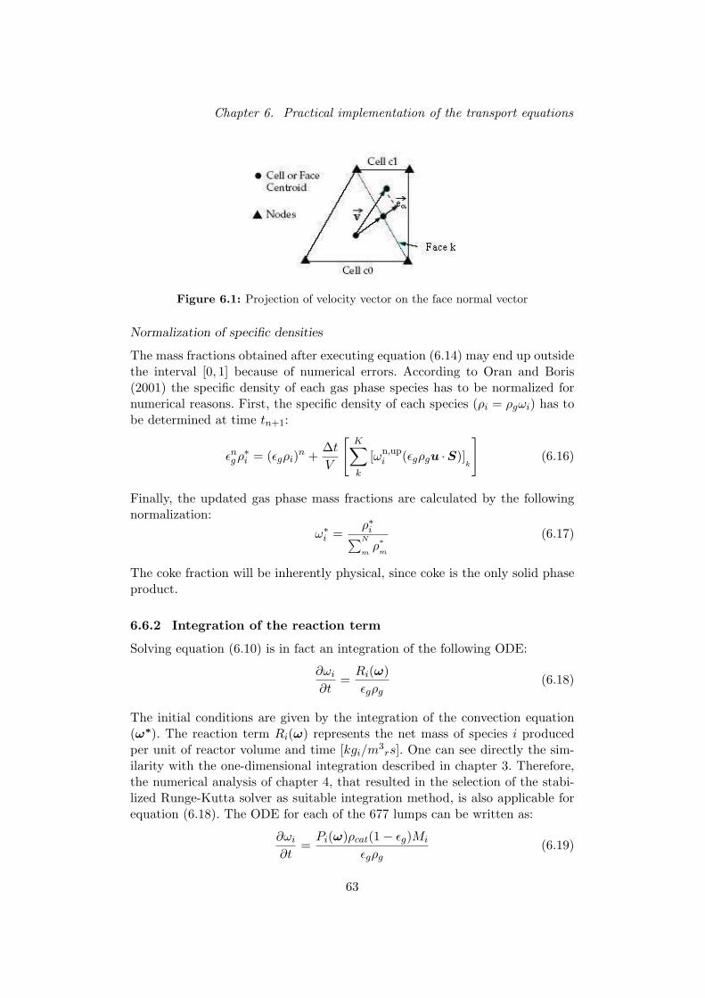
Chapter 6. Practical implementation of the transport equations
Figure 6.1: Projection of velocity vector on the face normal vector
Normalization of specific densities
The mass fractions obtained after executing equation (6.14) may end up outsidethe interval [0, 1] because of numerical errors. According to Oran and Boris(2001) the specific density of each gas phase species has to be normalized fornumerical reasons. First, the specific density of each species (ρi = ρgωi) has tobe determined at time tn+1:
εng ρ∗i = (εgρi)n +
∆t
V
[K∑k
[ωn,upi (εgρgu ·S)]
k
](6.16)
Finally, the updated gas phase mass fractions are calculated by the followingnormalization:
ω∗i =
ρ∗i∑N
mρ∗
m
(6.17)
The coke fraction will be inherently physical, since coke is the only solid phaseproduct.
6.6.2 Integration of the reaction term
Solving equation (6.10) is in fact an integration of the following ODE:
∂ωi
∂t=
Ri(ω)εgρg
(6.18)
The initial conditions are given by the integration of the convection equation(ω∗). The reaction term Ri(ω) represents the net mass of species i producedper unit of reactor volume and time [kgi/m3
rs]. One can see directly the sim-ilarity with the one-dimensional integration described in chapter 3. Therefore,the numerical analysis of chapter 4, that resulted in the selection of the stabi-lized Runge-Kutta solver as suitable integration method, is also applicable forequation (6.18). The ODE for each of the 677 lumps can be written as:
∂ωi
∂t=
Pi(ω)ρcat(1− εg)Mi
εgρg(6.19)
63

Chapter 6. Practical implementation of the transport equations
Pi is the net production rate of species i in moles per unit of catalyst massand time. The mass fractions of the inert species steam and nitrogen do notundergo reaction, therefore no reaction integration has to be performed forthese components. The amount of coke that deposits on the catalyst is foundby solving
∂yc
∂t= Pc(ω) (6.20)
where yc represents the mass of coke per mass of catalyst. Pc(ω) is thus the netproduction rate in mass coke per unit catalyst mass and time.
The simultaneous solution of system (6.19)-(6.20) yields the mass fractions ofthe lumps and the coke after reaction. In integrating the reaction equations(6.19)-(6.20) for the three dimensional simulation, the general behavior remainssimilar to the reactor balance (3.4) in the one-dimensional simulation of chap-ter 3 since the right-hand sides differ only by a constant factor. It was shown inchapter 4 that the stabilized Runge-Kutta solver was the most efficient solverfor problem type (3.4). Therefore, the code of Sommeijer et al. (1998) has beenused to integrate system (6.19)-(6.20) over the time-interval ∆t that has beenderived by the three-dimensional CFL criterion (6.14). In this code, the vari-able time steps and the number of RKC-stages are selected to obtain stableintegration and to reach the desired time-accuracy.
The gas phase mass fractions have to be renormalized after each reaction in-tegration because a certain amount of mass disappears from the gas phase toreappear as coke in the solid phase:
ωn+1i =
ωn+1i∑N
mωn+1
m
(6.21)
6.7 Overview of the solution method for the transportequations
In this section, a general overview is given of the interaction between Flu-ent and the subroutines that solve the transport equations for the species. Ascheme is given in Figure 6.2. The first step is basically the same as in the one-dimensional version of Quintana-Solorzano et al. (2005) and consists of readingthe input data. In order to perform a three-dimensional simulation just the ki-netic parameters, species boundary conditions and the individual properties ofthe components have to be read. The riser geometry, catalyst properties, globalfluid properties and the boundary conditions for the two phases are part of theFluent simulation and can be communicated with the external subroutines. Theitems read in this first step are:
• Inlet composition of the fluid entering the nozzles.
64

Chapter 6. Practical implementation of the transport equations
• Thermodynamics of the fluid mixture: the coefficients of the specificheat and the standard enthalpy of formation of each lump as given inequation (5.51).
• Molar mass of each component.• Activation energy and exponential prefactors for each single-event rate
coefficient.• Lumping coefficients for each global reaction type.
After reading this information, the mass fraction field has to be initialized overthe entire reactor. This step will be discussed in more detail in chapter 7.Using the current mass fractions, the properties of the global fluid mixture areupdated. The density is defined according to relation (5.44) and is practicallyimplemented as a define property function in Fluent.
After Fluent has updated the properties, the balances on the solid and fluid mix-ture are solved. As indicated in the scheme, the source terms for the continuityequations and the solid energy equation are calculated using the differences incomposition resulting from the last integration of the species continuity equa-tions. The source terms will be introduced in Fluent with a define sourcefunction. After these Fluent solution steps, a check for convergence is made.
Once a solution sequence for the global balances has been executed by Fluent,the integration of the species continuity equations will start, using a subroutinethat is called from Fluent with a define execute at end function. This UDFis executed at the end of each Fluent iteration and makes it possible to insert theintegration of the species transport equations in the Fluent segregated solvingsequence. Basically, this subroutine consists of a cell loop in which the coupledset of species continuity equations for each cell is solved by the following threesteps:
1. Selection of the integration time step ∆t on the basis of the CFL-criterion for the cell, see equation (6.14).
2. The convection step will be executed, using equation (6.11) for the Ngas phase components and equation (6.12) for cokes. This step ends withthe normalization of the gas phase mass fractions.
3. Integration of the coupled set of reaction balances (6.19)-(6.20) withthe stabilized Runge-Kutta solver. This set of ODEs will be integratedfrom t = 0 to t = ∆t and the initial mass fractions are these obtainedafter the convection step. The calculation of the net production ratesis identical to this in the reaction loop given in Figure 3.2. The finalpart in this third step is again the normalization of the gas phase massfractions.
It must be remarked that a Gauss-Seidel-style integration is used. The inte-gration of the transport equations of a certain cell can use an upwind massfraction that has been found in the current iteration cycle, because the updatefrom ωn to ωn+1 occurs immediately for this cell. The opposite would be a
65
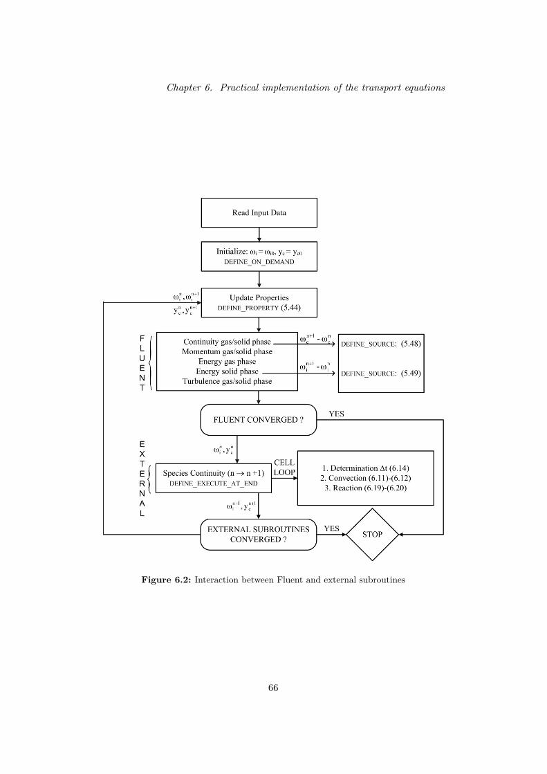
Chapter 6. Practical implementation of the transport equations
Figure 6.2: Interaction between Fluent and external subroutines
66
Chapter 6. Practical implementation of the transport equations
Jacobi technique in which the updates are executed only after the entire cellloop is performed.
After the entire cell loop, a check for convergence of the species continuityequations will made. Convergence is achieved if the variation in time of themass fractions of each component can be neglected. This means that the timederivative of equations (6.1)-(6.2) must remain small or for each cell must hold:
Ri(ω)−∇ · (εgρgωiu) ≈ 0 ∀ i = 1, . . . , N (6.22)Rc(ω)−∇ · (εsρsycv) ≈ 0 (6.23)
According to the discretized sequence as described above, convergence is prac-tically achieved if:
Gas:(εgρgωi)n+1 − (εgρgωi)∗
∆t− 1
V
[K∑k
[ωn,upi (εgρgu ·S)]
k
]≈ 0 (6.24)
Coke:(εsρsyc)n+1 − (εsρsyc)∗
∆t− 1
V
[K∑k
[yn,upc (εsρsv ·S)]
k
]≈ 0 (6.25)
The first term in these equations corresponds with the net production rateand the second term represents the net change in cell mass due to convection.Although convection and reaction are integrated sequentially, convergence isbased on the time-dependency of the entire transport equation. Convergence ina cell is achieved if the net mass flux of each species entering this cell, disappearsby chemical reaction.
The iteration cycle of Figure 6.2 must be executed until both global balances(Fluent) and species continuity balances have converged.
6.8 Conclusions
In this chapter, the solution method for the transport equations of the gasphase components and coke is presented. An operator-splitting technique, inwhich convection and reaction are integrated sequentially, was chosen in order toapply a suitable solver for the reaction term. The convection term is calculatedusing a first order upwind method and the reaction term is integrated withthe stabilized Runge-Kutta solver as outlined in chapter 4. The integration ofthe transport equations was embedded in the Fluent solution sequence andusing the appropriate user defined functions, communication between Fluentand external subroutines was provided.
67

PART III
SIMULATION RESULTS
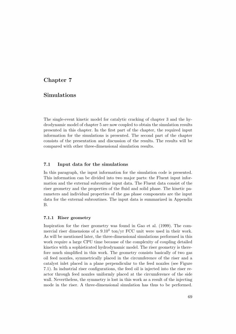
Chapter 7
Simulations
The single-event kinetic model for catalytic cracking of chapter 3 and the hy-drodynamic model of chapter 5 are now coupled to obtain the simulation resultspresented in this chapter. In the first part of the chapter, the required inputinformation for the simulations is presented. The second part of the chapterconsists of the presentation and discussion of the results. The results will becompared with other three-dimensional simulation results.
7.1 Input data for the simulations
In this paragraph, the input information for the simulation code is presented.This information can be divided into two major parts: the Fluent input infor-mation and the external subroutine input data. The Fluent data consist of theriser geometry and the properties of the fluid and solid phase. The kinetic pa-rameters and individual properties of the gas phase components are the inputdata for the external subroutines. The input data is summarized in AppendixB.
7.1.1 Riser geometry
Inspiration for the riser geometry was found in Gao et al. (1999). The com-mercial riser dimensions of a 9.104 ton/yr FCC unit were used in their work.As will be mentioned later, the three-dimensional simulations performed in thiswork require a large CPU time because of the complexity of coupling detailedkinetics with a sophisticated hydrodynamic model. The riser geometry is there-fore much simplified in this work. The geometry consists basically of two gasoil feed nozzles, symmetrically placed in the circumference of the riser and acatalyst inlet placed in a plane perpendicular to the feed nozzles (see Figure7.1). In industrial riser configurations, the feed oil is injected into the riser re-actor through feed nozzles uniformly placed at the circumference of the sidewall. Nevertheless, the symmetry is lost in this work as a result of the injectingmode in the riser. A three-dimensional simulation has thus to be performed.
69
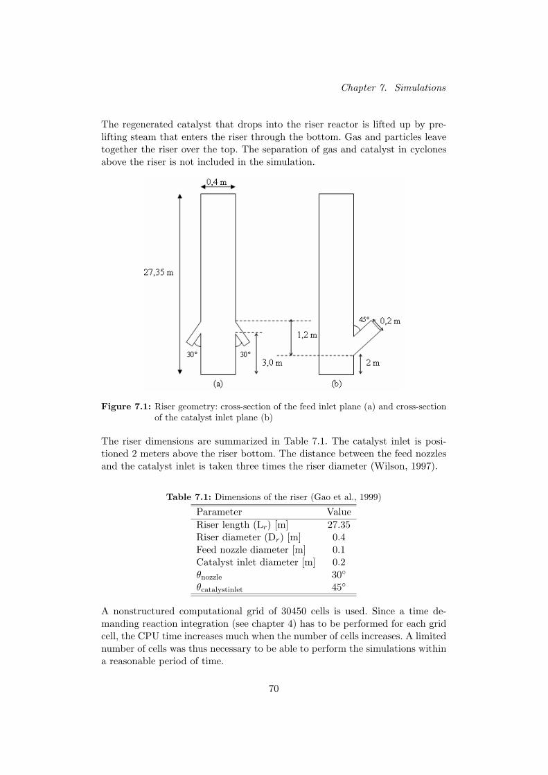
Chapter 7. Simulations
The regenerated catalyst that drops into the riser reactor is lifted up by pre-lifting steam that enters the riser through the bottom. Gas and particles leavetogether the riser over the top. The separation of gas and catalyst in cyclonesabove the riser is not included in the simulation.
Figure 7.1: Riser geometry: cross-section of the feed inlet plane (a) and cross-sectionof the catalyst inlet plane (b)
The riser dimensions are summarized in Table 7.1. The catalyst inlet is posi-tioned 2 meters above the riser bottom. The distance between the feed nozzlesand the catalyst inlet is taken three times the riser diameter (Wilson, 1997).
Table 7.1: Dimensions of the riser (Gao et al., 1999)
Parameter ValueRiser length (Lr) [m] 27.35Riser diameter (Dr) [m] 0.4Feed nozzle diameter [m] 0.1Catalyst inlet diameter [m] 0.2θnozzle 30
θcatalystinlet 45
A nonstructured computational grid of 30450 cells is used. Since a time de-manding reaction integration (see chapter 4) has to be performed for each gridcell, the CPU time increases much when the number of cells increases. A limitednumber of cells was thus necessary to be able to perform the simulations withina reasonable period of time.
70

Chapter 7. Simulations
7.1.2 Properties of the catalyst and global fluid phase
The properties of the catalyst are summarized in Table 7.2. This informationwas taken from Gao et al. (1999).
Table 7.2: Catalyst properties (Gao et al., 1999)
Parameter ValueDensity (ρs) [kg/m3] 1500Average Particle diameter (dp) [µm] 65Specific Heat (cp) [J/kgK] 1003Thermal conductivity (k) [W/mK] 2Maximum packing limit (εs,max) [-] 0.63Coefficient of restitution (ess) [-] 0.9
The global properties of the gas phase are summarized in Table 7.3. As indicatedin chapter 5, the gas phase density and molar weight are adopted during thecalculation for the changing gas composition. The viscosity (Quintana-Solorzanoet al., 2005), specific heat and thermal conductivity (Perry and Green, 1997) areassumed constant, regardless of the composition of the gas phase. The specificheat was assumed constant, because it is not possible to implement a user-defined specific heat in Fluent. In this work, the specific heat was taken as anaveraged value of the heat capacity values found in Quintana-Solorzano et al.(2005). In the latter work, cp,gas varied from 3200 J/kgK in the bottom of theriser to 2400 J/kgK in the top of the riser.
Table 7.3: Gas phase properties (Quintana-Solorzano et al., 2005; Perry and Green,1997)
Parameter ValueSpecific Heat (cp) [J/kgK] 2800Shear viscosity (µ) [105kg/ms] 1.1Thermal conductivity (k) [W/mK] 0.024
7.1.3 Kinetic parameters
In chapter 3, the single-event kinetic modeling of catalytic cracking was de-scribed. The single-event rate coefficients depend on the catalyst, but they re-main invariant to the feed composition. Given a certain catalyst, the rate coeffi-cients can be determined by experiments with simple model components. Theseexperiments have been performed and described by Dewachtere (1997). Addi-tional experiments for the coke precursors were provided by Quintana-Solorzanoet al. (2005). The experiments resulted in a total number of 59 single-event ratecoefficients of the following form:
ki = AiTe(−EiRT
) (7.1)
71

Chapter 7. Simulations
The experimental values of the pre-exponential factors A and the activation en-ergies E are given in Quintana-Solorzano et al. (2005) and will not be presentedin this work.
The lumping coefficients, that have to be inserted in the reaction rate equations,are determined from the reaction network generation algorithm for the givenfeed composition. These coefficients can also be found in Quintana-Solorzanoet al. (2005) and they are read in the data input step.
7.1.4 Individual properties of the lumps
Since most of the global properties of the gas phase are assumed constant, theonly property that has to be read for each lump, is the molar weight. Thesemolar weights are presented in Quintana-Solorzano et al. (2005) and will beused for the density calculation of the gas phase mixture.
Despite the fact that the specific heat of the gas phase is assumed constant, thethermodynamic properties of each lump have to be known for the calculationof the energy source term (5.49). This implies that the standard enthalpy offormation and the coefficients cp0, cp1 and cp2 of the temperature dependentspecific heat as given in (5.51), also have to be known for each lump.
Experimental thermodynamic data for hydrocarbons are hard to find. Ben-son (1976) developed a group contribution method to estimate the standardenthalpy of formation ∆H0
f and temperature dependent molar heat capacity.The principle of this method is that each carbon atom in a given hydrocarbonmolecule amounts a certain contribution to the enthalpy of formation and thespecific heat. The value of this contribution depends only on the type of theconsidered carbon atom and on the type of its neighboring carbon atoms. Thecomputation of these thermodynamic properties is implemented in the networkgeneration algorithm. For a given hydrocarbon molecule, the type of each carbonatom and its neighboring carbon atoms can easily be found using the compactvector formulation of the molecule. In Dewachtere (1997), the thermodynamicproperties have been calculated with the network generation algorithm and theresulting thermodynamic data file is read in the data input step of this work.
7.1.5 Boundary conditions
In this paragraph, the boundary conditions for the different inlet sections of theriser are presented.
Inlet conditions
The two gas oil feed nozzles, the catalyst inlet and the prelifting steam inlet areconsidered separately. The boundary conditions are identical for the two feednozzles and therefore only the boundary condition for feed nozzle 1 is presented.
72

Chapter 7. Simulations
The mass flows of steam, nitrogen, gas oil and the catalyst through the differentinlets are presented in Table 7.4. In industrial FCC units, the entering catalystis accompanied by some remaining combustion gases formed in the regener-ation section. External aeration can be ensured in the catalyst standpipe byinjecting a supplemental gas medium, such as air, steam, nitrogen or fuel gas(Sadeghbeigi, 1995). In this work, these gases are for simplicity considered tobe nitrogen gas. The gas oil and catalyst mass flows are taken from the workof Gao et al. (1999). The steam velocity (and consequently its mass flow) hasbeen raised as compared to Gao et al. (1999) in order to avoid that catalystleaves the reactor via the riser bottom. No information on the catalyst-nitrogenratio at the catalyst inlet was found in literature. Therefore, the mass flow ofnitrogen was chosen in such a way that the catalyst volume fraction equals0.2 at the catalyst inlet boundary. This choice is midway between a downwardparticle velocity that is too high and a particle loading that is too high. Gasand catalyst velocities are assumed identical at the catalyst inlet boundary (slipvelocity = 1).
The catalyst-gasoil ratio is an important parameter in the FCC proces. It is theratio between the inlet catalyst mass flow and the total gas oil inlet mass flow atthe nozzles. In this work, this ratio equals 3.7 (as in Gao et al. (1999)), whichis also comparable to the values used in other three-dimensional simulations(Theologos and Markatos, 1993; Dewachtere, 1997).
Table 7.4: Boundary conditions for the simulation of an FCC-riser (Gao et al., 1999)
Variable Steam inlet Catalyst inlet Feed nozzle 1Ggasoil [kg/s] 0 0 1.3417Gsteam [kg/s] 0.152 0 0Gnitrogen [kg/s] 0 0.02 0Gcatalyst [kg/s] 0 9.9316 0Gas temperature [K] 875 875 698Catalyst temperature [K] 875 875 698
The inlet temperatures at each boundary are also based on the operating con-ditions given in Gao et al. (1999). As can be seen in Table 7.4, temperaturesare identical for both phases at the catalyst inlet. In comparison with one-dimensional simulations (e.g. as in chapter 3), both catalyst and gas oil inlettemperatures are rather low. To obtain realistic gasoline yields, one-dimensionalsimulations generally require higher temperatures and catalyst to oil ratios. Theexternal pressure at the riser outlet was assumed to be uniformly equal to theatmospheric pressure.
73
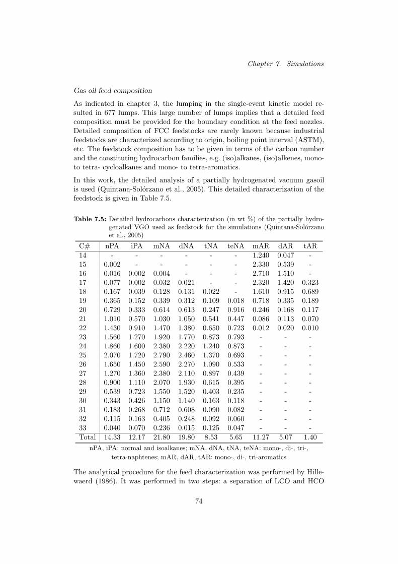
Chapter 7. Simulations
Gas oil feed composition
As indicated in chapter 3, the lumping in the single-event kinetic model re-sulted in 677 lumps. This large number of lumps implies that a detailed feedcomposition must be provided for the boundary condition at the feed nozzles.Detailed composition of FCC feedstocks are rarely known because industrialfeedstocks are characterized according to origin, boiling point interval (ASTM),etc. The feedstock composition has to be given in terms of the carbon numberand the constituting hydrocarbon families, e.g. (iso)alkanes, (iso)alkenes, mono-to tetra- cycloalkanes and mono- to tetra-aromatics.
In this work, the detailed analysis of a partially hydrogenated vacuum gasoilis used (Quintana-Solorzano et al., 2005). This detailed characterization of thefeedstock is given in Table 7.5.
Table 7.5: Detailed hydrocarbons characterization (in wt %) of the partially hydro-genated VGO used as feedstock for the simulations (Quintana-Solorzanoet al., 2005)
C# nPA iPA mNA dNA tNA teNA mAR dAR tAR14 - - - - - - 1.240 0.047 -15 0.002 - - - - - 2.330 0.539 -16 0.016 0.002 0.004 - - - 2.710 1.510 -17 0.077 0.002 0.032 0.021 - - 2.320 1.420 0.32318 0.167 0.039 0.128 0.131 0.022 - 1.610 0.915 0.68919 0.365 0.152 0.339 0.312 0.109 0.018 0.718 0.335 0.18920 0.729 0.333 0.614 0.613 0.247 0.916 0.246 0.168 0.11721 1.010 0.570 1.030 1.050 0.541 0.447 0.086 0.113 0.07022 1.430 0.910 1.470 1.380 0.650 0.723 0.012 0.020 0.01023 1.560 1.270 1.920 1.770 0.873 0.793 - - -24 1.860 1.600 2.380 2.220 1.240 0.873 - - -25 2.070 1.720 2.790 2.460 1.370 0.693 - - -26 1.650 1.450 2.590 2.270 1.090 0.533 - - -27 1.270 1.360 2.380 2.110 0.897 0.439 - - -28 0.900 1.110 2.070 1.930 0.615 0.395 - - -29 0.539 0.723 1.550 1.520 0.403 0.235 - - -30 0.343 0.426 1.150 1.140 0.163 0.118 - - -31 0.183 0.268 0.712 0.608 0.090 0.082 - - -32 0.115 0.163 0.405 0.248 0.092 0.060 - - -33 0.040 0.070 0.236 0.015 0.125 0.047 - - -Total 14.33 12.17 21.80 19.80 8.53 5.65 11.27 5.07 1.40
nPA, iPA: normal and isoalkanes; mNA, dNA, tNA, teNA: mono-, di-, tri-,tetra-naphtenes; mAR, dAR, tAR: mono-, di-, tri-aromatics
The analytical procedure for the feed characterization was performed by Hille-waerd (1986). It was performed in two steps: a separation of LCO and HCO
74
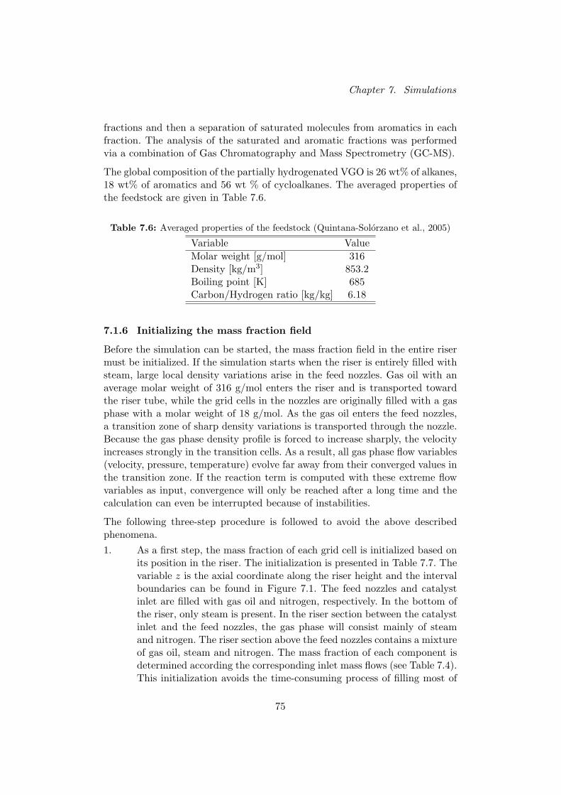
Chapter 7. Simulations
fractions and then a separation of saturated molecules from aromatics in eachfraction. The analysis of the saturated and aromatic fractions was performedvia a combination of Gas Chromatography and Mass Spectrometry (GC-MS).
The global composition of the partially hydrogenated VGO is 26 wt% of alkanes,18 wt% of aromatics and 56 wt % of cycloalkanes. The averaged properties ofthe feedstock are given in Table 7.6.
Table 7.6: Averaged properties of the feedstock (Quintana-Solorzano et al., 2005)
Variable ValueMolar weight [g/mol] 316Density [kg/m3] 853.2Boiling point [K] 685Carbon/Hydrogen ratio [kg/kg] 6.18
7.1.6 Initializing the mass fraction field
Before the simulation can be started, the mass fraction field in the entire risermust be initialized. If the simulation starts when the riser is entirely filled withsteam, large local density variations arise in the feed nozzles. Gas oil with anaverage molar weight of 316 g/mol enters the riser and is transported towardthe riser tube, while the grid cells in the nozzles are originally filled with a gasphase with a molar weight of 18 g/mol. As the gas oil enters the feed nozzles,a transition zone of sharp density variations is transported through the nozzle.Because the gas phase density profile is forced to increase sharply, the velocityincreases strongly in the transition cells. As a result, all gas phase flow variables(velocity, pressure, temperature) evolve far away from their converged values inthe transition zone. If the reaction term is computed with these extreme flowvariables as input, convergence will only be reached after a long time and thecalculation can even be interrupted because of instabilities.
The following three-step procedure is followed to avoid the above describedphenomena.1. As a first step, the mass fraction of each grid cell is initialized based on
its position in the riser. The initialization is presented in Table 7.7. Thevariable z is the axial coordinate along the riser height and the intervalboundaries can be found in Figure 7.1. The feed nozzles and catalystinlet are filled with gas oil and nitrogen, respectively. In the bottom ofthe riser, only steam is present. In the riser section between the catalystinlet and the feed nozzles, the gas phase will consist mainly of steamand nitrogen. The riser section above the feed nozzles contains a mixtureof gas oil, steam and nitrogen. The mass fraction of each component isdetermined according the corresponding inlet mass flows (see Table 7.4).This initialization avoids the time-consuming process of filling most of
75

Chapter 7. Simulations
the riser section with the feed components by convection. Moreover, thebuild-up of extreme flow variables — as a consequence of the progressingtransition zone — has been avoided.
Table 7.7: Initialized mass fraction field
Gas phase component
Position Steam Nitrogen GasoilFeed nozzle 0 0 1Catalyst inlet 0 1 0z < 2 m 1 0 02 m < z < 3 m 0.884 0.116 0z > 3 m 0.053 0.007 0.940
2. An abrupt discontinuity in the mass fraction field now arises at z = 3m. Therefore, a certain amount of iteration loops is performed withoutaccounting for reaction of the gas phase components. The mass fractionfield evolves into a continuous profile and the density variations becomesmooth.
3. On the converged mass fraction field that has been found by applyingpure convection, reaction is now superposed. Starting from the gas oilconcentration of the feed — diluted with inert steam and nitrogen — ina given cell of the riser (with z > 3 m), the time-dependent transportequation, including reaction, is now integrated.
7.2 Results and discussion
The simulation results are presented in this section. Predicted flow and reactionvariables are given in the form of contours at selected planes of the riser reactor,as shown in the Figures 7.2 to 7.11. Figure 7.2 gives a global overview of gasolinemass fraction and the fluid temperature in a cross section of the feed inlet plane.The gasoline mass fraction increases at the beginning of the riser and reachesa maximum value at an axial coordinate of about 9 m. The maximum value isfound half-way the riser, because the simulations presented in this work havenot yet converged. The required CPU-time for the simulations, as performedso far, amounted to about 35 days. The gasoline profiles as shown in Figure7.2 (i) can be explained by the fact that a first-order upwind convection isused. In the first step of each transport equation integration (as discussed inthe operator splitting of chapter 6), the components of the reacting mixture aretransported with the global fluid flow. In the second step the time-dependentreaction is submitted on the mass fractions obtained after convection. Since theconvection integration is performed by a first-order upwind method, each mass
76

Chapter 7. Simulations
fraction is only influenced by its corresponding mass fraction in the immediateneighboring cells. It takes thus a long time before the components in the bottomof the riser, which result from convection and reaction, have been transportedto the end of the riser. On Figure 7.2 (i) can be seen that the gasoline that isproduced near the nozzles, has only been convected to an axial coordinate ofabout 9 meters. The maximum gasoline mass fractions at z = 9 m have yet tobe transported to the riser outlet, using the first-order upwind convection.
It is therefore not useful to present the simulation results in the upper part ofthe riser, because they have no physical meaning in this stage of the calculations.In what follows, the simulation results will be presented for axial coordinateslower than 10 m. Although the simulations are not yet converged in the lowerpart of the riser, the profile can up to 10 m be considered as reliable for thefollowing reasons. First of all, the profiles presented in this work correspondwell with the results presented in literature (Theologos and Markatos, 1993;Gao et al., 1999). Furthermore, the conversion at one-third of the riser lengthis realistic compared to values in literature (Gao et al., 1999; Landeghem et al.,1996). A last argument is given by the solution procedure itself. The convectionis calculated by an upstream method and the velocity vectors are almost alluniformly directed upwards in riser section above the nozzles (see also Figure7.10). The variables of a given grid cell are therefore hardly influenced by thecells above it.
The fluid temperature profile of Figure 7.2 (ii) seems realistic over the entireriser length. The temperature drops from about 795 K at z = 3.5 m (where fluidand catalyst temperatures are almost equal, see Figure 7.16) to 750 K at the riseroutlet. The temperature drop of 45 K is similar to values in literature (Wilson,1997). The fact that the temperature profile agrees rather well with publishedprofiles — although the mass fractions are not yet converged — is surprising,but may be explained by the fact that the temperature drop calculation is basedon the reaction rates (see equation (5.49)) rather than on the mass fractions.
Despite the fact the Single-Event Kinetic model — which includes 678 lumps —has been applied in this work, the lumps have been gathered into the categoriesHCO, LCO, gasoline, LPG and fuel gas for the presentation of the results inthis chapter. This approach has the advantage that a comparison can be madewith simulations that use a limited amount of lumps. The disadvantage is thatless details can be observed. The categories HCO, LCO, gasoline, LPG and fuelgas consist of lumps with a carbon number interval of respectively 40-20, 20-13,12-5, 4-3 and 2-1.
77

Chapter 7. Simulations
Figure 7.2: Cross section of the riser: contour plots in a vertical plane through thefeed nozzles of (i) gasoline mass fraction and (ii) fluid temperature
78

Chapter 7. Simulations
The mass fraction distributions of gasoline, LCO and HCO in a vertical crosssection through the feed nozzles (which will be called “feed inlet plane” in whatfollows) are presented in Figure 7.3 (limited to a height of 9.5 m). As the HCOconcentration decreases along the axial riser coordinate, the gasoline mass frac-tion increases. The LCO mass fraction first decreases and then again increases.The gasoline and LPG mass fraction distributions in a vertical cross sectionthrough the catalyst inlet (which will be called “catalyst inlet plane” in whatfollows) are presented in Figure 7.4 (i) and Figure 7.5 (i) respectively. The LPGand fuel gas (which is not presented here) mass fraction profiles exhibit basi-cally the same distribution as gasoline and therefore only the three-dimensionalgasoline production profiles will be described in the following paragraphs.
Figure 7.3: Vertical cross section of the feed inlet plane: (i) gasoline, (ii) LCO and(iii) HCO mass fraction as a function of the axial coordinate of the riser
The mass fraction profiles are not uniform for a given axial coordinate. It can beseen that a low gasoline concentration arises in the vicinity of the feed nozzles.Higher gasoline mass fractions arise in the center of the riser and particularlyin the catalyst inlet plane. The gasoline mass fractions near the wall, as shownin Figures 7.6 (z = 3.3 m)1 and 7.4 (i), are the highest peaks in the entire riser.
1. In the horizontal cross sections of the risers, N1 and N2 represent the feed nozzles and Crepresents the catalyst inlet.
79
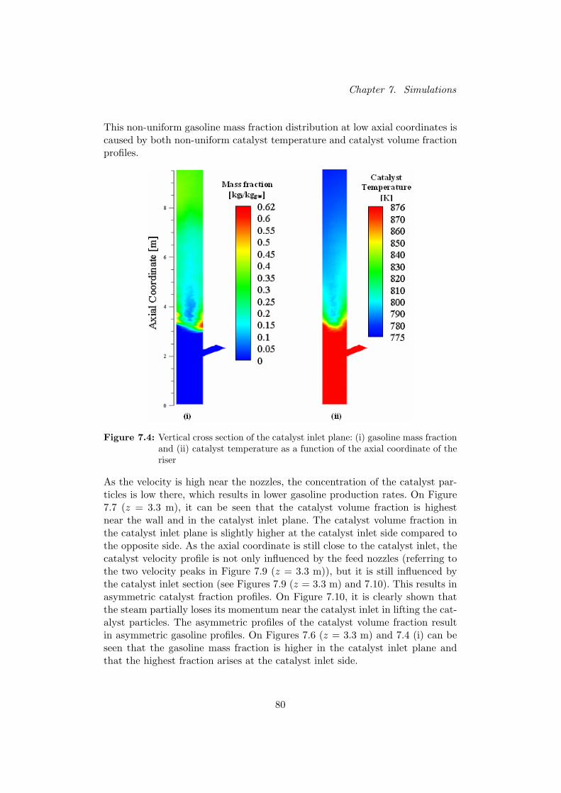
Chapter 7. Simulations
This non-uniform gasoline mass fraction distribution at low axial coordinates iscaused by both non-uniform catalyst temperature and catalyst volume fractionprofiles.
Figure 7.4: Vertical cross section of the catalyst inlet plane: (i) gasoline mass fractionand (ii) catalyst temperature as a function of the axial coordinate of theriser
As the velocity is high near the nozzles, the concentration of the catalyst par-ticles is low there, which results in lower gasoline production rates. On Figure7.7 (z = 3.3 m), it can be seen that the catalyst volume fraction is highestnear the wall and in the catalyst inlet plane. The catalyst volume fraction inthe catalyst inlet plane is slightly higher at the catalyst inlet side compared tothe opposite side. As the axial coordinate is still close to the catalyst inlet, thecatalyst velocity profile is not only influenced by the feed nozzles (referring tothe two velocity peaks in Figure 7.9 (z = 3.3 m)), but it is still influenced bythe catalyst inlet section (see Figures 7.9 (z = 3.3 m) and 7.10). This results inasymmetric catalyst fraction profiles. On Figure 7.10, it is clearly shown thatthe steam partially loses its momentum near the catalyst inlet in lifting the cat-alyst particles. The asymmetric profiles of the catalyst volume fraction resultin asymmetric gasoline profiles. On Figures 7.6 (z = 3.3 m) and 7.4 (i) can beseen that the gasoline mass fraction is higher in the catalyst inlet plane andthat the highest fraction arises at the catalyst inlet side.
80
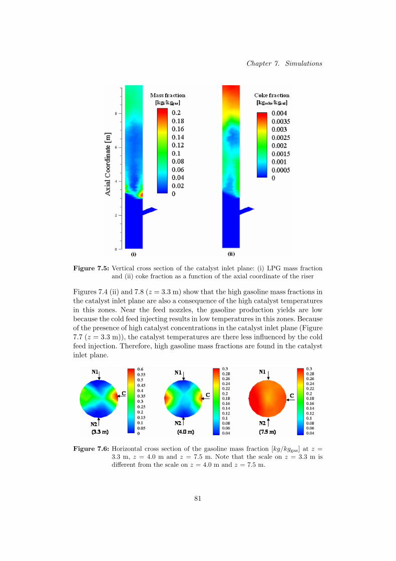
Chapter 7. Simulations
Figure 7.5: Vertical cross section of the catalyst inlet plane: (i) LPG mass fractionand (ii) coke fraction as a function of the axial coordinate of the riser
Figures 7.4 (ii) and 7.8 (z = 3.3 m) show that the high gasoline mass fractions inthe catalyst inlet plane are also a consequence of the high catalyst temperaturesin this zones. Near the feed nozzles, the gasoline production yields are lowbecause the cold feed injecting results in low temperatures in this zones. Becauseof the presence of high catalyst concentrations in the catalyst inlet plane (Figure7.7 (z = 3.3 m)), the catalyst temperatures are there less influenced by the coldfeed injection. Therefore, high gasoline mass fractions are found in the catalystinlet plane.
Figure 7.6: Horizontal cross section of the gasoline mass fraction [kg/kggas] at z =3.3 m, z = 4.0 m and z = 7.5 m. Note that the scale on z = 3.3 m isdifferent from the scale on z = 4.0 m and z = 7.5 m.
81

Chapter 7. Simulations
Figure 7.7: Horizontal cross section of the catalyst volume fraction [m3cat/m3
r] at z =3.3 m, z = 4.0 m and z = 7.5 m. Note that the scale on z = 3.3 m isdifferent from the scale on z = 4.0 m and z = 7.5 m.
As the axial coordinate increases, the velocity profiles are less influenced by thecatalyst inlet and the feed nozzles. Figure 7.9 (z = 4.0 m) shows that the catalystvelocity profile is almost entirely symmetric in the catalyst inlet plane. Thedifference in catalyst volume fraction at both sides of the catalyst inlet planethus diminishes, but the catalyst volume fraction is still low near the feed nozzles(Figure 7.6 (z = 4.0 m)). The temperature differences in the horizontal crosssection at z = 4.0 m (Figure 7.8) have been reduced because of the more uniformcatalyst distribution, but the catalyst temperature is still significantly lowernear the feed nozzles. The influence of the slightly asymmetric catalyst volumefraction distribution on the catalyst temperature can now be seen more clearlythan at z = 3.3 m. The gasoline concentration profile at the axial coordinateof 4 meters (Figure 7.6) can be explained by the relevant cracking reactionconditions: the catalyst temperature and the catalyst concentration (as hasbeen done for z = 3.3 m).
Figure 7.8: Horizontal cross section of the catalyst temperature [K] at z = 3.3 m, z= 4.0 m and z = 7.5 m. Note that the scale on z = 3.3 m is different fromthe scale on z = 4.0 m and z = 7.5 m.
Figures 7.6 to 7.9 (z = 7.5 m) show that the distributions higher-up in theriser and further away from the feed and catalyst efflux regions become moreuniform. The velocity profiles evolve to the typical parabolic form (see alsoFigure 7.10), which is also reported by Das et al. (2003). The catalyst volumefraction and temperature (see also Figure 7.4(ii)) inhomogeneities are therefore
82
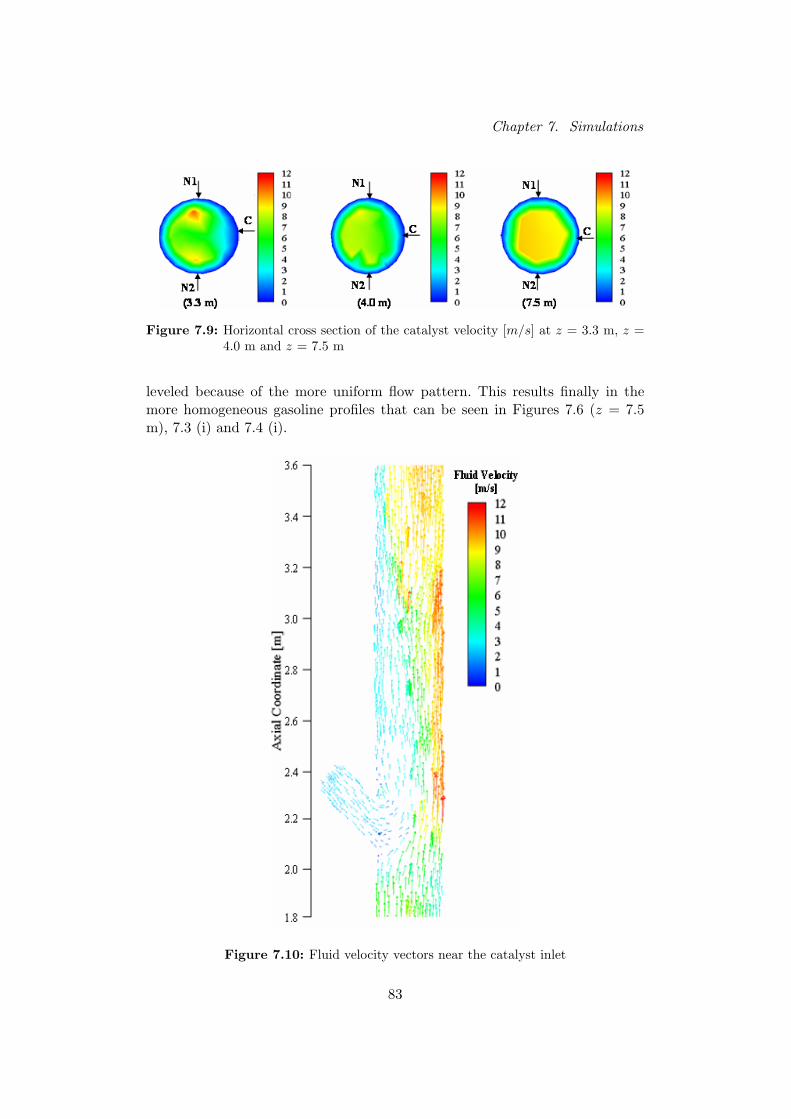
Chapter 7. Simulations
Figure 7.9: Horizontal cross section of the catalyst velocity [m/s] at z = 3.3 m, z =4.0 m and z = 7.5 m
leveled because of the more uniform flow pattern. This results finally in themore homogeneous gasoline profiles that can be seen in Figures 7.6 (z = 7.5m), 7.3 (i) and 7.4 (i).
Figure 7.10: Fluid velocity vectors near the catalyst inlet
83

Chapter 7. Simulations
The fact that the catalyst volume fraction becomes more uniform higher-up inthe riser has an influence on the coke fraction distribution in the riser (Daset al., 2003). In Figure 7.5 (ii), the coke fraction (per unit of catalyst mass) ispresented in a vertical cross section through the catalyst inlet. For low axialcoordinates, the coke fraction is higher near the wall, which corresponds withthe high catalyst volume fraction at the side of the catalyst inlet plane. As thecatalyst volume distribution becomes more uniform for higher axial coordinates,the coke distribution is gradually spread over the cross section of the riser.
Figure 7.7 shows clearly that the catalyst volume fraction is low near the feednozzles and higher in the zone between the two feed nozzles. These resultscorrespond with the catalyst distributions presented in literature (Gao et al.,1999; Theologos and Markatos, 1993). Nevertheless, the radial distributions ofthe catalyst particles obtained in this work show some shortcomings as com-pared to literature. According to Das et al. (2003) and Gao et al. (1999), thesolid volume fraction is significantly higher near the entire wall of the riser as aconsequence of the low velocities near the wall. Das et al. (2003) even reportsa sudden increase of the solids fraction in the core region at one-third of theriser height. Although a detailed two phase turbulence model has been appliedin this work, these radial variations have not been found until now. This possi-ble shortcoming can be attributed to the rather low number of grid cells. Thecoarse grid is believed to have a negative influence only on the near-wall region,because large local variations arise in this zone.
At axial coordinates above 7 meters, there is an increase in the gas and solidvelocity due to an increase in the production of the lighter products gasoline,LPG and fuel gas. These phenomena are also reported in Das et al. (2003). Thevolume of the gas mixture increases as reactions continue and this is reflectedby a lower gas phase density, as shown in Figure 7.11 (i). Due to the expansionof the fluid mixture, its velocity increases and the catalyst phase is draggedalong with the gas phase. The increase of the catalyst phase velocity is clearlyseen in Figure 7.11 (ii). The increase in the velocity is also for a small part dueto the pressure drop along the axial coordinate. Lower pressures allow the gasphase to expand and increase the solid velocity due to a higher drag force.
The fluid density and catalyst velocity profiles shown in Figure 7.11 are oncemore presented in Figures 7.12 and 7.13 respectively. On these figures, the areaaveraged values are shown for different axial coordinates. Figure 7.12 teachesthat the gas density increases between 3 and 3.5 meters, because of the injectionof the heavy gas oil. For these axial coordinates, the heavy HCO and LCO arenot yet dispersed over the entire horizontal cross section (see Figure 7.14 (z= 3.2 m)), because they have just entered the riser and every contact withthe fresh catalyst (particularly in the catalyst inlet plane with high catalystconcentrations) results in instantaneous cracking.
84
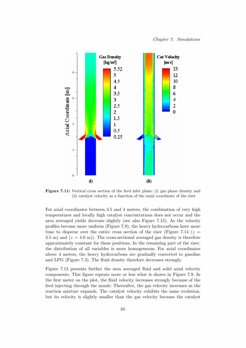
Chapter 7. Simulations
Figure 7.11: Vertical cross section of the feed inlet plane: (i) gas phase density and(ii) catalyst velocity as a function of the axial coordinate of the riser
For axial coordinates between 3.5 and 4 meters, the combination of very hightemperatures and locally high catalyst concentrations does not occur and thearea averaged yields decrease slightly (see also Figure 7.15). As the velocityprofiles become more uniform (Figure 7.9), the heavy hydrocarbons have moretime to disperse over the entire cross section of the riser (Figure 7.14 (z =3.5 m) and (z = 4.0 m)). The cross-sectional averaged gas density is thereforeapproximately constant for these positions. In the remaining part of the riser,the distribution of all variables is more homogeneous. For axial coordinatesabove 4 meters, the heavy hydrocarbons are gradually converted to gasolineand LPG (Figure 7.3). The fluid density therefore decreases strongly.
Figure 7.13 presents further the area averaged fluid and solid axial velocitycomponents. This figure repeats more or less what is shown in Figure 7.9. Inthe first meter on the plot, the fluid velocity increases strongly because of thefeed injecting through the nozzle. Thereafter, the gas velocity increases as thereaction mixture expands. The catalyst velocity exhibits the same evolution,but its velocity is slightly smaller than the gas velocity because the catalyst
85
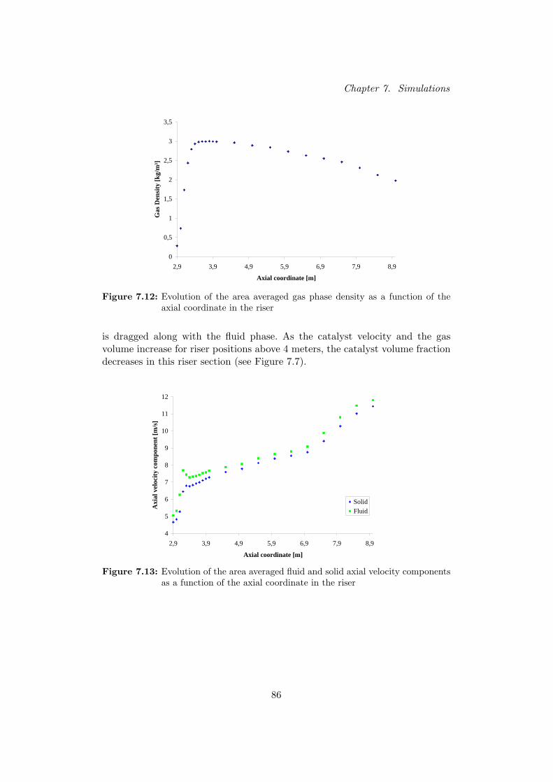
Chapter 7. Simulations
0
0,5
1
1,5
2
2,5
3
3,5
2,9 3,9 4,9 5,9 6,9 7,9 8,9
Axial coordinate [m]
Gas
Den
sity
[kg/
m³]
Figure 7.12: Evolution of the area averaged gas phase density as a function of theaxial coordinate in the riser
is dragged along with the fluid phase. As the catalyst velocity and the gasvolume increase for riser positions above 4 meters, the catalyst volume fractiondecreases in this riser section (see Figure 7.7).
4
5
6
7
8
9
10
11
12
2,9 3,9 4,9 5,9 6,9 7,9 8,9
Axial coordinate [m]
Axi
al v
eloc
ity
com
pone
nt [
m/s
]
SolidFluid
Figure 7.13: Evolution of the area averaged fluid and solid axial velocity componentsas a function of the axial coordinate in the riser
86

Chapter 7. Simulations
Figure 7.14: Horizontal cross section of the HCO mass fraction [kg/kggas] at z = 3.2m, z = 3.5 m and z = 4.0 m
The global observations made for the above described figures are also found inFigure 7.15, where the area averaged mass fractions of gasoline, LCO, HCO andLPG are shown as a function of the axial coordinate. For each position, the massfractions are averaged over the cross section of the riser (nozzles not included).The fuel gas has not been presented in this figure because its mass fraction isalmost negligible. The coke fraction presented in this figure is calculated on totalgas phase mass basis in order to be able to compare the coke production withthe other product yields. This fraction is for each axial coordinate calculatedas:
ωc =ρsεs
ρgεgyc (7.2)
with yc obtained by solving the coke transport equations, described in chapter 6.
At an axial coordinate of 3 meters, the gas phase still consists mainly of steamand nitrogen, which explains that all mass fractions are low there. At the startof the feed nozzles, the HCO- and LCO-profiles start to build up. At locationswhere a combination of high temperature and high (fresh!) catalyst concen-tration occurs, the heavy hydrocarbons that have entered the riser, crack in-stantaneously to gasoline. The HCO mass fraction is therefore not everywhereimmediately built up to the high concentration of the feed (see also Figure 7.14(z = 3.2 m) and (z = 3.5 m)). The gasoline mass fraction thus increases stronglyin the first decimeters of the riser. For axial coordinates between 3.5 and 4 me-ters, the high peaks of catalyst fraction and temperature have disappeared.While the heavy hydrocarbons are concentrated near the wall between 3 and3.5 meters, they are now more uniformly spread over the riser section (see Fig-ure 7.14 (z = 4.0 m)). Once the heavy hydrocarbons (HCO and LCO) profileshave completely built up (at z = 4 m), LCO and HCO are cracked graduallyto gasoline, LPG and coke. From 3.5 to 6.5 meters, specifically LCO is crackedinto gasoline. From 6.5 meters on, HCO is cracked to gasoline, LPG, coke andalso LCO. The formation of coke results in a deactivation of the catalyst.
The successive fall and rise of the LCO mass fraction in the beginning of the riserwas already shown in Figure 7.3 (ii) and in Figure 3.4 of the one-dimensional
87

Chapter 7. Simulations
simulation of Quintana-Solorzano et al. (2005). Gao et al. (1999) obtained com-parable profiles for LCO. At z = 9 m, the mass fraction curves of all reactioncomponents become already more stagnant. Despite the fact that the three-dimensional profiles of LPG appear to be similar than these of gasoline (seeFigure 7.5), Figure 7.15 learns that the production of LPG (and also fuel gas)is slower that the gasoline production, because LPG has to be formed fromcracking of gasoline.
0,00
0,05
0,10
0,15
0,20
0,25
0,30
0,35
0,40
0,45
0,50
3,0 4,0 5,0 6,0 7,0 8,0 9,0
Axial coordinate [m]
Mas
s fr
acti
on [
kg/k
g gas
]
0,0
0,1
0,2
0,3
0,4
0,5
0,6
0,7
HC
O M
ass
frac
tion
[kg
/kg g
as]
Gasoline
LCO
LPG
Coke
Conversion
HCO
Figure 7.15: Evolution of the area averaged conversion and mass fractions on totalgas phase mass basis of HCO, LCO, gasoline, LPG and coke
In order to calculate the conversion, the product yields Zj are calculated ac-cording to Das et al. (2003):
Zj =ωj
ωc +∑
k ωk(7.3)
In this definition, the mass fraction summation is performed for HCO, LCO,gasoline, LPG and fuel gas. Remark that the yields have to account for thecoke that has left the gas phase. The conversion, as shown in Figure 7.15, isnow calculated as in Quintana-Solorzano et al. (2005) (see equation (3.11)):
1− ZHCO − ZLCO (7.4)
In Figure 7.15, it can be seen that the conversion at the beginning of the feednozzles starts from a high value. This somewhat distorted image is a conse-quence of the vigorous cracking of the heavy hydrocarbons in the inlet zone ofthe riser, while the HCO and LCO concentrations have not yet built up.
88
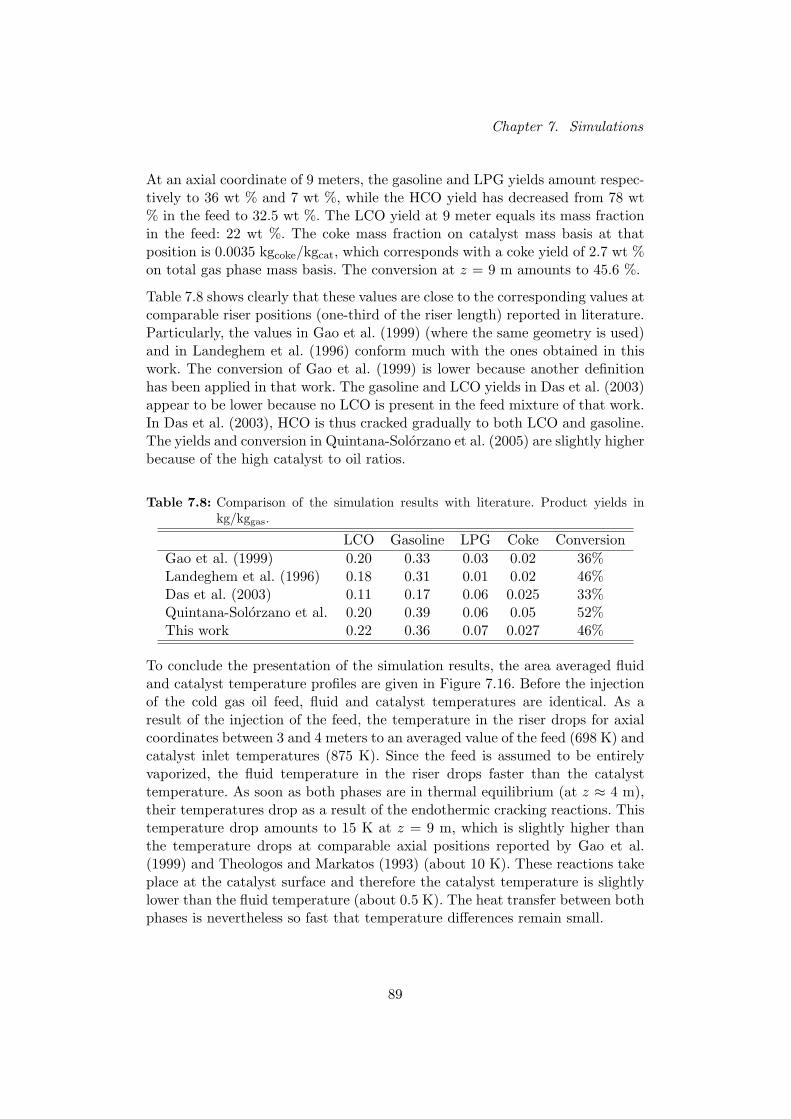
Chapter 7. Simulations
At an axial coordinate of 9 meters, the gasoline and LPG yields amount respec-tively to 36 wt % and 7 wt %, while the HCO yield has decreased from 78 wt% in the feed to 32.5 wt %. The LCO yield at 9 meter equals its mass fractionin the feed: 22 wt %. The coke mass fraction on catalyst mass basis at thatposition is 0.0035 kgcoke/kgcat, which corresponds with a coke yield of 2.7 wt %on total gas phase mass basis. The conversion at z = 9 m amounts to 45.6 %.
Table 7.8 shows clearly that these values are close to the corresponding values atcomparable riser positions (one-third of the riser length) reported in literature.Particularly, the values in Gao et al. (1999) (where the same geometry is used)and in Landeghem et al. (1996) conform much with the ones obtained in thiswork. The conversion of Gao et al. (1999) is lower because another definitionhas been applied in that work. The gasoline and LCO yields in Das et al. (2003)appear to be lower because no LCO is present in the feed mixture of that work.In Das et al. (2003), HCO is thus cracked gradually to both LCO and gasoline.The yields and conversion in Quintana-Solorzano et al. (2005) are slightly higherbecause of the high catalyst to oil ratios.
Table 7.8: Comparison of the simulation results with literature. Product yields inkg/kggas.
LCO Gasoline LPG Coke ConversionGao et al. (1999) 0.20 0.33 0.03 0.02 36%Landeghem et al. (1996) 0.18 0.31 0.01 0.02 46%Das et al. (2003) 0.11 0.17 0.06 0.025 33%Quintana-Solorzano et al. 0.20 0.39 0.06 0.05 52%This work 0.22 0.36 0.07 0.027 46%
To conclude the presentation of the simulation results, the area averaged fluidand catalyst temperature profiles are given in Figure 7.16. Before the injectionof the cold gas oil feed, fluid and catalyst temperatures are identical. As aresult of the injection of the feed, the temperature in the riser drops for axialcoordinates between 3 and 4 meters to an averaged value of the feed (698 K) andcatalyst inlet temperatures (875 K). Since the feed is assumed to be entirelyvaporized, the fluid temperature in the riser drops faster than the catalysttemperature. As soon as both phases are in thermal equilibrium (at z ≈ 4 m),their temperatures drop as a result of the endothermic cracking reactions. Thistemperature drop amounts to 15 K at z = 9 m, which is slightly higher thanthe temperature drops at comparable axial positions reported by Gao et al.(1999) and Theologos and Markatos (1993) (about 10 K). These reactions takeplace at the catalyst surface and therefore the catalyst temperature is slightlylower than the fluid temperature (about 0.5 K). The heat transfer between bothphases is nevertheless so fast that temperature differences remain small.
89

Chapter 7. Simulations
775
785
795
805
815
825
835
845
855
865
875
2,9 3,9 4,9 5,9 6,9 7,9 8,9
Axial coordinate [m]
Tem
pera
ture
[K
]
Gas temperatureCatalyst temperature
Figure 7.16: Evolution of the area averaged fluid and catalyst temperature as a func-tion of the axial coordinate
7.3 Conclusions
A three-dimensional gas-solid riser simulation has been performed and the re-sults are presented in this chapter. The riser geometry was taken from Gaoet al. (1999) and as a consequence of the asymmetric catalyst inlet, the simu-lations have a three-dimensional character. The boundary conditions are basedon the work of Gao et al. (1999) and the feed composition was taken fromQuintana-Solorzano et al. (2005).
The three-dimensional results are presented in the form of contours at selectedplanes of the riser reactor. The evolution of different relevant area averagedvariables as a function of the axial coordinate have also been shown. Despitethe fact that the simulations have not yet converged, the profiles presented inthis work correspond well with the simulation results presented in literature(for riser positions until 9 m).
90
Chapter 8
Conclusions and future work
In this work, a three-dimensional gas-solid simulation of the riser of a catalyticcracking unit has been performed. The three-dimensional character of the simu-lation arises from the riser geometry, which consists basically of two feed nozzlesand one catalyst inlet positioned in a plane perpendicular with regard to thesenozzles.
In order to perform these simulations, a complex kinetic model has been com-bined with a complete three-dimensional hydrodynamic model. The kineticmodel applied in this work has been developed at the Laboratorium voor Petro-chemische Techniek at the University of Ghent. This Single-Event MicroKineticmodel includes elementary reaction steps for 677 lumps and it gives a funda-mental prediction of the coke formation in the riser. Because of the fundamentalcharacter of the model, the rate coefficients are feed-independent.
The applied hydrodynamic model consists of the continuity, momentum, en-ergy and turbulence balances for both the gas and the solid phase, closed witha number of constitutive relations. The model is completed by the continu-ity equations for the gas phase components and the coke that deposits on thecatalyst. In this work, the model equations are partially solved by the commer-cial simulation package Fluent and partially by a user-defined program, thatinteracts with Fluent. As the number of components in the Single-Event Mi-croKinetic model exceeds the maximum number of continuity equations thatcan be solved by Fluent, the individual continuity equations have been solvedexternally with regard to Fluent.
The transport equations for the gas phase components and cokes have been in-tegrated by applying a first-order operator splitting technique. In this method,the convection part and the reaction part of the transport equations are solvedseparately in a two-step sequence. The convection part has been integratedwith a first-order upwind method. The reaction step is integrated with the sta-bilized Runge-Kutta solver, which has been selected on the basis of its superiorefficiency in comparison with other integration methods.
91

Chapter 8. Conclusions and future work
The simulation results, as presented in this report, have not yet reached a con-verged state. Nevertheless, the solution profiles — as performed so far — corre-spond well with the simulation results presented in literature. While most FluidCatalytic Cracking simulations rely on kinetic models using drastic lumping oron simple hydrodynamic models, in this work a detailed fundamental kineticmodel is combined with a complete three-dimensional hydrodynamic model,which forms the merit of this work.
Future work can be done concerning four topics. First of all, extra simulationscan be undertaken using the current simulation code. In performing these newsimulations, parameters could be varied, the riser geometry could be made moredetailed or a finer grid could be implemented at the feed inlet zone in contrastwith the other riser sections.
Although several concepts have been introduced in this work that reduce the re-quired CPU time for the simulations significantly (such as the operator splittingintegration technique and the selection of the efficient stabilized Runge-Kuttamethod for the reaction integration), the complete CPU time will amount toabout three months. A useful project is thus to further reduce the required sim-ulation time. Since the convection integration appears to be the limiting factor,a multigrid approach can be suggested.
Finally, two extensions to this work can be suggested. In industrial units, thefeed enters the riser in a liquefied state. A vaporization model for the hydrocar-bon feed could thus be developed and implemented. The second project consistsof extending the transport equations, as integrated in this work, with diffusionmodeling for each gas phase component.
92

PART IV
APPENDICES

Appendix A
Model equations for reactive two-phase gas-solid flow
A.1 Model equations
• Gas phase continuity equation
∂
∂t(εgρg) +∇ · (εgρgu) = −mgs (A.1)
• Solid phase continuity equation
∂
∂t(εsρs) +∇ · (εsρsv) = mgs (A.2)
• Gas phase momentum equation
∂
∂t(εgρgu)+∇ · (εgρguu) = −εg∇pg +∇ · ¯τg−βu(u−v)+ εgρgg (A.3)
• Solid phase momentum equation
∂
∂t(εsρsv) +∇ · (εsρsvv) = −εs∇pg −∇pg +∇ · ¯τs + βu(u− v) + εsρsg
(A.4)• Gas phase energy equation
∂
∂t(εgρgEg) +∇ · (εgρguHg) = ∇ · (¯τg ·u)−∇ · (−εgkg∇Tg)
− βT (Tg − Ts) + εgρgg ·u(A.5)
• Solid phase energy equation
∂
∂t(εsρsEs) +∇ · (εsρsvHs) = ∇ · (¯τs ·v)−∇ · (−εsks∇Ts) + βT (Tg − Ts)
+ εsρsg ·v −N∑i
∆Hi,fRi
(A.6)
94
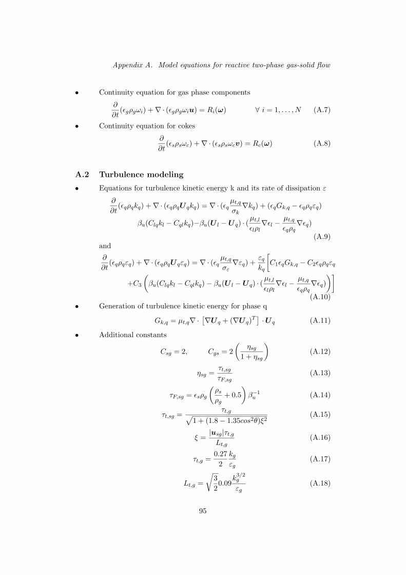
Appendix A. Model equations for reactive two-phase gas-solid flow
• Continuity equation for gas phase components
∂
∂t(εgρgωi) +∇ · (εgρgωiu) = Ri(ω) ∀ i = 1, . . . , N (A.7)
• Continuity equation for cokes
∂
∂t(εsρsωc) +∇ · (εsρsωcv) = Rc(ω) (A.8)
A.2 Turbulence modeling
• Equations for turbulence kinetic energy k and its rate of dissipation ε
∂
∂t(εqρqkq) +∇ · (εqρqU qkq) = ∇ · (εq
µt,q
σk∇kq) + (εqGk,q − εqρqεq)
βu(Clqkl − Cqlkq)−βu(U l −U q) · (µt,l
εlρl∇εl −
µt,q
εqρq∇εq)
(A.9)and
∂
∂t(εqρqεq) +∇ · (εqρqU qεq) = ∇ · (εq
µt,q
σε∇εq) +
εq
kq
[C1εqGk,q − C2εqρqεq
+C3
(βu(Clqkl − Cqlkq)− βu(U l −U q) · (
µt,l
εlρl∇εl −
µt,q
εqρq∇εq)
)](A.10)
• Generation of turbulence kinetic energy for phase q
Gk,q = µt,q∇ ·[∇U q + (∇U q)T
]·U q (A.11)
• Additional constants
Csg = 2, Cgs = 2(
ηsg
1 + ηsg
)(A.12)
ηsg =τt,sg
τF,sg(A.13)
τF,sg = εsρg
(ρs
ρg+ 0.5
)β−1
u (A.14)
τt,sg =τt,g√
1 + (1.8− 1.35cos2θ)ξ2(A.15)
ξ =|usg|τt,g
Lt,g(A.16)
τt,g =0.272
kg
εg(A.17)
Lt,g =
√320.09
k3/2g
εg(A.18)
95

Appendix A. Model equations for reactive two-phase gas-solid flow
• Turbulent viscosity µt for each phase q
µt,q = 0.09ρq
k2q
εq(A.19)
A.3 Constitutive equations
A.3.1 Total energy and enthalpy
• Enthalpy of formation of each component
∆Hi,f = ∆H0i,f +
∫ T
T0
cp,idT (A.20)
cp,i = cp0,i + cp1,iT + cp2,iT2 (A.21)
• Gas phase total specific enthalpy
Hg = hg +12u ·u (A.22)
hg = cp,gTg (A.23)
• Gas phase specific free energy
Eg = Hg −pg
ρg= eg +
12u ·u (A.24)
• Solid phase total specific enthalpy
Hs = hs +32θ +
12v ·v (A.25)
hs = cp,sTs (A.26)
• Solid phase specific free energy
Es = Hs −ps
ρs= es +
32θ +
12v ·v (A.27)
A.3.2 Molecular flux of momentum
• Gas phase stress-strain tensor
¯τg = εg(µg + µt,g)[∇u +∇uT
]+ εg
[λg −
23(µg + µt,g)
]∇ ·u ¯I (A.28)
• Gas phase stress-strain tensor
¯τs = εs(µs + µt,s)[∇v +∇vT
]+ εs
[λs −
23(µs + µt,s)
]∇ ·v ¯I, (A.29)
96
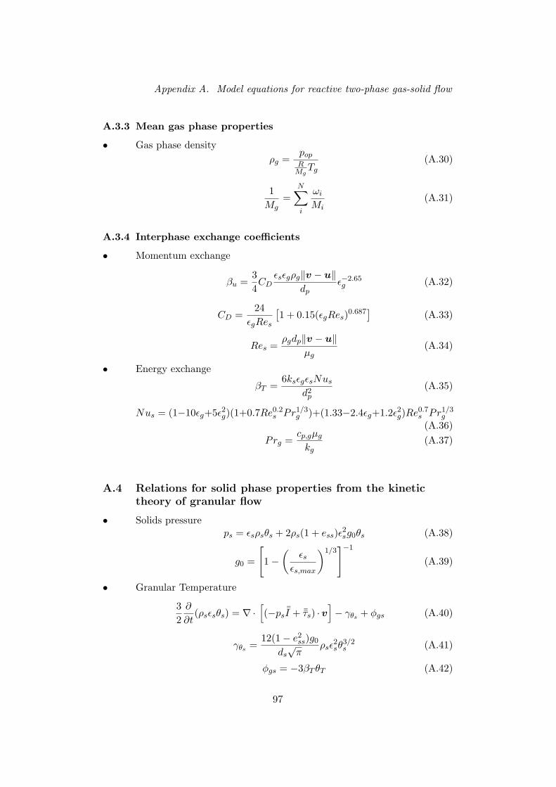
Appendix A. Model equations for reactive two-phase gas-solid flow
A.3.3 Mean gas phase properties
• Gas phase densityρg =
pop
RMg
Tg
(A.30)
1Mg
=N∑i
ωi
Mi(A.31)
A.3.4 Interphase exchange coefficients
• Momentum exchange
βu =34CD
εsεgρg‖v − u‖dp
ε−2.65g (A.32)
CD =24
εgRes
[1 + 0.15(εgRes)0.687
](A.33)
Res =ρgdp‖v − u‖
µg(A.34)
• Energy exchange
βT =6ksεgεsNus
d2p
(A.35)
Nus = (1−10εg+5ε2g)(1+0.7Re0.2s Pr1/3
g )+(1.33−2.4εg+1.2ε2g)Re0.7s Pr1/3
g
(A.36)Prg =
cp,gµg
kg(A.37)
A.4 Relations for solid phase properties from the kinetictheory of granular flow
• Solids pressureps = εsρsθs + 2ρs(1 + ess)ε2sg0θs (A.38)
g0 =
[1−
(εs
εs,max
)1/3]−1
(A.39)
• Granular Temperature
32
∂
∂t(ρsεsθs) = ∇ ·
[(−ps
¯I + ¯τs) ·v]− γθs + φgs (A.40)
γθs =12(1− e2
ss)g0
ds√
πρsε
2sθ
3/2s (A.41)
φgs = −3βT θT (A.42)
97

Appendix A. Model equations for reactive two-phase gas-solid flow
• Solid shear stressesµs = µs,col + µs,kin (A.43)
µs,col =45εsρsdpg0(1 + ess)
(θs
π
)1/2
(A.44)
µs,kin =10dpρs
√θsπ
96εs(1− ess)g0
[1 +
45g0εs(1 + ess)
]2
(A.45)
λs =43εsρsdpg0(1 + ess)
(θs
π
)1/2
(A.46)
98
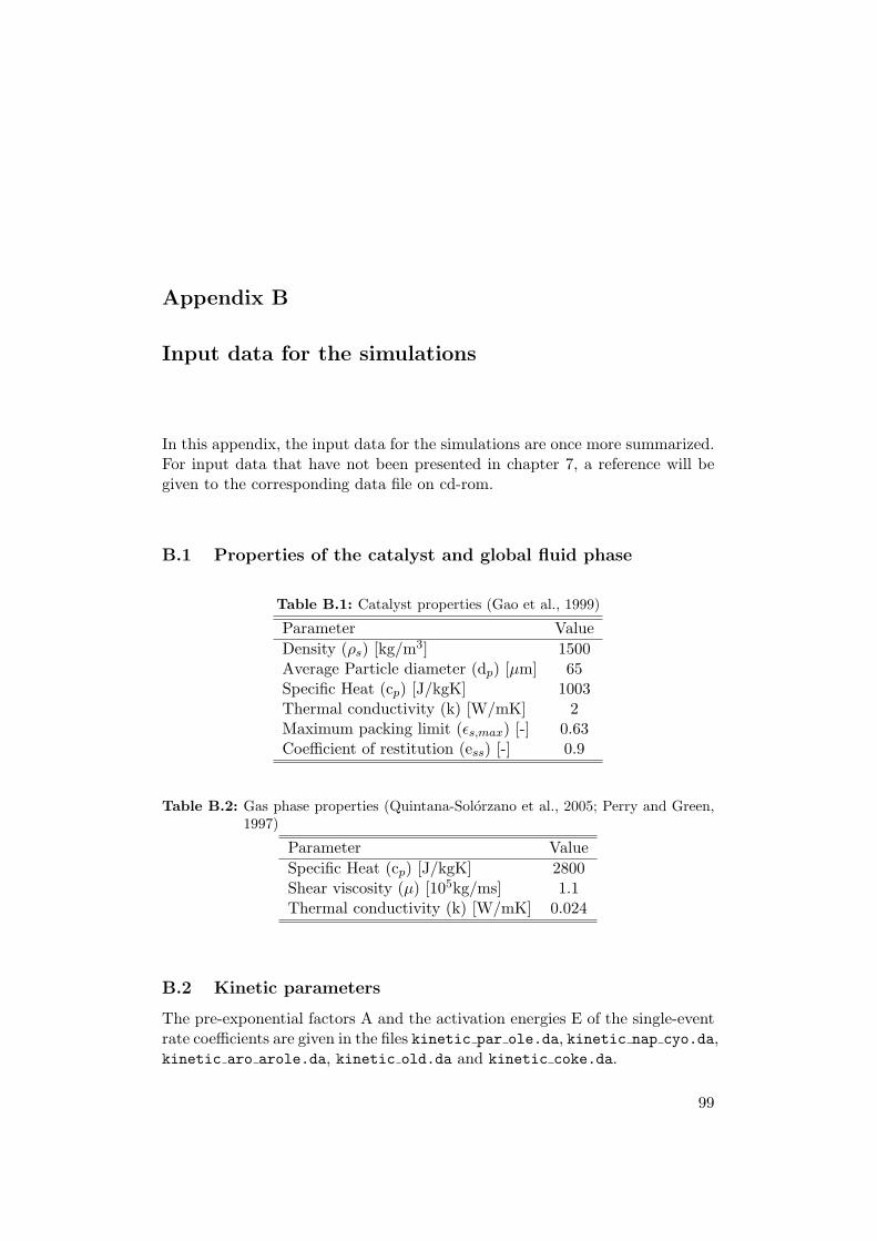
Appendix B
Input data for the simulations
In this appendix, the input data for the simulations are once more summarized.For input data that have not been presented in chapter 7, a reference will begiven to the corresponding data file on cd-rom.
B.1 Properties of the catalyst and global fluid phase
Table B.1: Catalyst properties (Gao et al., 1999)
Parameter ValueDensity (ρs) [kg/m3] 1500Average Particle diameter (dp) [µm] 65Specific Heat (cp) [J/kgK] 1003Thermal conductivity (k) [W/mK] 2Maximum packing limit (εs,max) [-] 0.63Coefficient of restitution (ess) [-] 0.9
Table B.2: Gas phase properties (Quintana-Solorzano et al., 2005; Perry and Green,1997)
Parameter ValueSpecific Heat (cp) [J/kgK] 2800Shear viscosity (µ) [105kg/ms] 1.1Thermal conductivity (k) [W/mK] 0.024
B.2 Kinetic parameters
The pre-exponential factors A and the activation energies E of the single-eventrate coefficients are given in the files kinetic par ole.da, kinetic nap cyo.da,kinetic aro arole.da, kinetic old.da and kinetic coke.da.
99
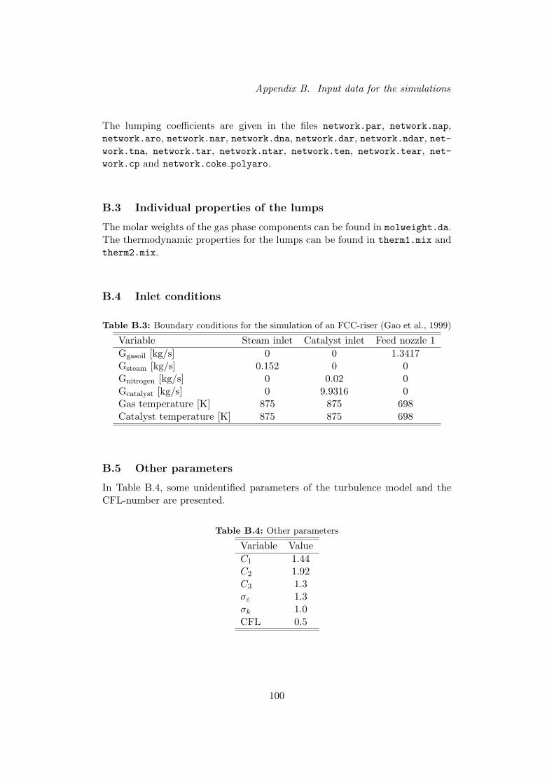
Appendix B. Input data for the simulations
The lumping coefficients are given in the files network.par, network.nap,network.aro, network.nar, network.dna, network.dar, network.ndar, net-work.tna, network.tar, network.ntar, network.ten, network.tear, net-work.cp and network.coke polyaro.
B.3 Individual properties of the lumps
The molar weights of the gas phase components can be found in molweight.da.The thermodynamic properties for the lumps can be found in therm1.mix andtherm2.mix.
B.4 Inlet conditions
Table B.3: Boundary conditions for the simulation of an FCC-riser (Gao et al., 1999)
Variable Steam inlet Catalyst inlet Feed nozzle 1Ggasoil [kg/s] 0 0 1.3417Gsteam [kg/s] 0.152 0 0Gnitrogen [kg/s] 0 0.02 0Gcatalyst [kg/s] 0 9.9316 0Gas temperature [K] 875 875 698Catalyst temperature [K] 875 875 698
B.5 Other parameters
In Table B.4, some unidentified parameters of the turbulence model and theCFL-number are presented.
Table B.4: Other parameters
Variable ValueC1 1.44C2 1.92C3 1.3σε 1.3σk 1.0CFL 0.5
100
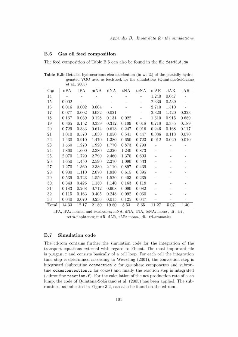
Appendix B. Input data for the simulations
B.6 Gas oil feed composition
The feed composition of Table B.5 can also be found in the file feed3 d.da.
Table B.5: Detailed hydrocarbons characterization (in wt %) of the partially hydro-genated VGO used as feedstock for the simulations (Quintana-Solorzanoet al., 2005)
C# nPA iPA mNA dNA tNA teNA mAR dAR tAR14 - - - - - - 1.240 0.047 -15 0.002 - - - - - 2.330 0.539 -16 0.016 0.002 0.004 - - - 2.710 1.510 -17 0.077 0.002 0.032 0.021 - - 2.320 1.420 0.32318 0.167 0.039 0.128 0.131 0.022 - 1.610 0.915 0.68919 0.365 0.152 0.339 0.312 0.109 0.018 0.718 0.335 0.18920 0.729 0.333 0.614 0.613 0.247 0.916 0.246 0.168 0.11721 1.010 0.570 1.030 1.050 0.541 0.447 0.086 0.113 0.07022 1.430 0.910 1.470 1.380 0.650 0.723 0.012 0.020 0.01023 1.560 1.270 1.920 1.770 0.873 0.793 - - -24 1.860 1.600 2.380 2.220 1.240 0.873 - - -25 2.070 1.720 2.790 2.460 1.370 0.693 - - -26 1.650 1.450 2.590 2.270 1.090 0.533 - - -27 1.270 1.360 2.380 2.110 0.897 0.439 - - -28 0.900 1.110 2.070 1.930 0.615 0.395 - - -29 0.539 0.723 1.550 1.520 0.403 0.235 - - -30 0.343 0.426 1.150 1.140 0.163 0.118 - - -31 0.183 0.268 0.712 0.608 0.090 0.082 - - -32 0.115 0.163 0.405 0.248 0.092 0.060 - - -33 0.040 0.070 0.236 0.015 0.125 0.047 - - -Total 14.33 12.17 21.80 19.80 8.53 5.65 11.27 5.07 1.40
nPA, iPA: normal and isoalkanes; mNA, dNA, tNA, teNA: mono-, di-, tri-,tetra-naphtenes; mAR, dAR, tAR: mono-, di-, tri-aromatics
B.7 Simulation code
The cd-rom contains further the simulation code for the integration of thetransport equations external with regard to Fluent. The most important fileis plugin.c and consists basically of a cell loop. For each cell the integrationtime step is determined according to Wesseling (2001), the convection step isintegrated (subroutine convection.c for gas phase components and subrou-tine cokesconvection.c for cokes) and finally the reaction step is integrated(subroutine reaction.f). For the calculation of the net production rate of eachlump, the code of Quintana-Solorzano et al. (2005) has been applied. The sub-routines, as indicated in Figure 3.2, can also be found on the cd-rom.
101

Bibliography
Anderson E., Bai Z., Bischof C., Blackford S., Demmel J., Dongarra J.,Du Croz J., Greenbaum A., Hammarling S., McKenney A. and SorensenD. (1999). LAPACK Users’ Guide. Society for Industrial and AppliedMathematics, Philadelphia, PA.
Barry D.A., Bajracharya K., Crapper M., Prommer H. and Cunningham C.J.(2000). Comparison of split-operator methods for solving coupled chemicalnon-equilibrium reaction/groundwater transport models. Mathematics andComputers in Simulation, 53, 113–127.
Benson S. (1976). Thermodynamical Kinetics. John Wiley & Sons, New York.
Benyahia S., Ortiz A. and Paredes J. (2003). Numerical Analysis of a ReactingGas/Solid Flow in the Riser Section of an Industrial Fluid Catalytic CrackingUnit. International Journal of Chemical Reactor Engineering, 1, 23–34.
Blom J.G. and Verwer J.G. (2000). A comparison of integration methods foratmospheric transport–chemistry problems. Journal of Computational andApplied Mathematics, 126, 381–396.
Brackx F. (2003). Wiskundige Analyse III. Cursus, Universiteit Gent, FaculteitIngenieurswetenschappen.
Cartwright J. and Piro O. (1992). The dynamics of Runge-Kutta methods.International Journal of Bifurcation and Chaos, 2, 427–449.
Das A.K., Baudrez E., Marin G.B. and Heynderickx G.J. (2003). Three-Dimensional Simulation of a Fluid Catalytic Cracking Riser Reactor.Industrial and Engineering Chemistry Research, 42, 2602–2617.
Dewachtere N.V. (1997). Single-Event Kinetische Modellering van het Kat-alytisch Kraken van Gasolie. Ph.D. thesis, Universiteit Gent, FaculteitToegepaste Wetenschappen, Vakgroep Chemische Proceskunde en Technis-che Chemie, Laboratorium voor Petrochemische Techniek.
102
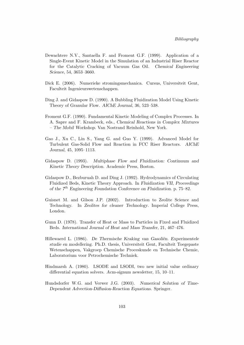
Bibliography
Dewachtere N.V., Santaella F. and Froment G.F. (1999). Application of aSingle-Event Kinetic Model in the Simulation of an Industrial Riser Reactorfor the Catalytic Cracking of Vacuum Gas Oil. Chemical EngineeringScience, 54, 3653–3660.
Dick E. (2006). Numerieke stromingsmechanica. Cursus, Universiteit Gent,Faculteit Ingenieurswetenschappen.
Ding J. and Gidaspow D. (1990). A Bubbling Fluidization Model Using KineticTheory of Granular Flow. AIChE Journal, 36, 523–538.
Froment G.F. (1990). Fundamental Kinetic Modeling of Complex Processes. InA. Sapre and F. Krambeck, eds., Chemical Reactions in Complex Mixtures– The Mobil Workshop. Van Nostrand Reinhold, New York.
Gao J., Xu C., Lin S., Yang G. and Guo Y. (1999). Advanced Model forTurbulent Gas-Solid Flow and Reaction in FCC Riser Reactors. AIChEJournal, 45, 1095–1113.
Gidaspow D. (1993). Multiphase Flow and Fluidization: Continuum andKinetic Theory Description. Academic Press, Boston.
Gidaspow D., Bezburuah D. and Ding J. (1992). Hydrodynamics of CirculatingFluidized Beds, Kinetic Theory Approach. In Fluidization VII, Proceedingsof the 7th Engineering Foundation Conference on Fluidization. p. 75–82.
Guisnet M. and Gilson J.P. (2002). Introduction to Zeolite Science andTechnology. In Zeolites for cleaner Technology. Imperial College Press,London.
Gunn D. (1978). Transfer of Heat or Mass to Particles in Fixed and FluidizedBeds. International Journal of Heat and Mass Transfer, 21, 467–476.
Hillewaerd L. (1986). De Thermische Kraking van Gasolien. Experimentelestudie en modellering. Ph.D. thesis, Universiteit Gent, Faculteit ToegepasteWetenschappen, Vakgroep Chemische Proceskunde en Technische Chemie,Laboratorium voor Petrochemische Techniek.
Hindmarsh A. (1980). LSODE and LSODI, two new initial value ordinarydifferential equation solvers. Acm-signum newsletter, 15, 10–11.
Hundsdorfer W.G. and Verwer J.G. (2003). Numerical Solution of Time-Dependent Advection-Diffusion-Reaction Equations. Springer.
103

Bibliography
Kim J. and Cho S.Y. (1997). Computation accuracy and efficiency of thetime-splitting method in solving atmospheric transport/chemistry equations.Atmospheric Environment, 31(15), 2215–2224.
Knio O.M., Najm H.N. and Wyckoff P.S. (1999). A Semi-implicit NumericalScheme for Reacting Flow: II. Stiff, Operator-Split Formulation. Journal ofComputational Physics, 154, 428–467.
Lambert J. (1990). Numerical Methods for Ordinary Differential Systems. TheInitial Value Problem. Wiley, Chichester.
Landeghem F.V., Nevicato D., Pitault I., Forissier M., Turlier P., Derouin C.and Bernard J. (1996). Fluid Catalytic Cracking: modelling of an industrialriser. Applied Catalysis A, 138, 381–405.
Lanser D. and Verwer J.G. (1999). Analysis of operator splitting foradvection–diffusion–reaction problems from air pollution modelling. Journalof Computational and Applied Mathematics, 111, 201–216.
Launder B. and Spalding D. (1972). Lectures in Mathematical Models ofTurbulence. Academic Press, London, England.
LeVeque R.J. and Yee H.C. (1990). A Study of Numerical Methods for Hyper-bolic Conservation Laws with Stiff Source Terms. Journal of ComputationalPhysics, 86, 187–210.
Lomax H., Pulliam T.H. and Zingg D.W. (2003). Fundamentals of Computa-tional Fluid Dynamics. Springer, New York.
Lun C., Savage S., Jeffrey D. and Chepurniy N. (1984). Kinetic Theories forGranular Flow: Inelastic Particles in Couette Flow and Slightly InelasticParticles in a General Flow Field. Journal of Fluid Mechanics, 140, 223–256.
Marin G. (2005). Chemische Reactoren: Principes en Toepassingen. Cursus,Universiteit Gent, Faculteit Ingenieurswetenschappen.
Najm H.N., Wyckoff P.S. and Knio O.M. (1998). A Semi-implicit NumericalScheme for Reacting Flow: I. Stiff Chemistry. Journal of ComputationalPhysics, 143, 381–402.
Oran E.S. and Boris J.P. (2001). Numerical Simulation of Reactive Flow.Cambridge University Press, Cambridge.
104
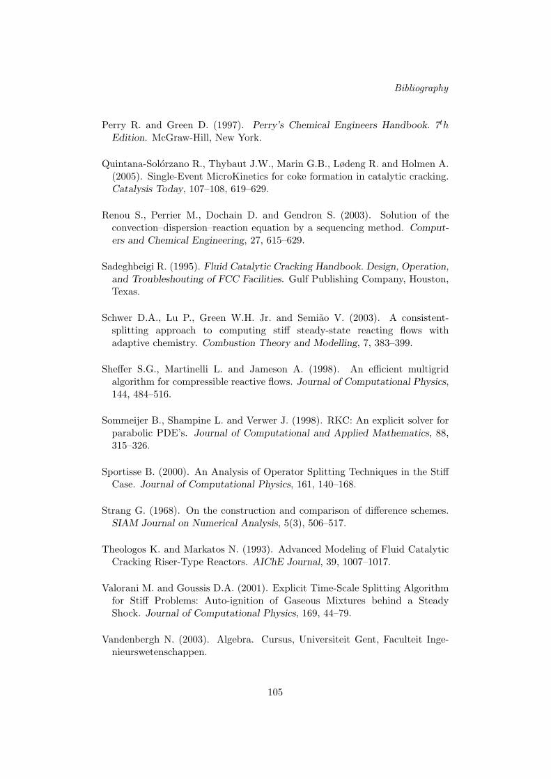
Bibliography
Perry R. and Green D. (1997). Perry’s Chemical Engineers Handbook. 7thEdition. McGraw-Hill, New York.
Quintana-Solorzano R., Thybaut J.W., Marin G.B., Lødeng R. and Holmen A.(2005). Single-Event MicroKinetics for coke formation in catalytic cracking.Catalysis Today, 107–108, 619–629.
Renou S., Perrier M., Dochain D. and Gendron S. (2003). Solution of theconvection–dispersion–reaction equation by a sequencing method. Comput-ers and Chemical Engineering, 27, 615–629.
Sadeghbeigi R. (1995). Fluid Catalytic Cracking Handbook. Design, Operation,and Troubleshouting of FCC Facilities. Gulf Publishing Company, Houston,Texas.
Schwer D.A., Lu P., Green W.H. Jr. and Semiao V. (2003). A consistent-splitting approach to computing stiff steady-state reacting flows withadaptive chemistry. Combustion Theory and Modelling, 7, 383–399.
Sheffer S.G., Martinelli L. and Jameson A. (1998). An efficient multigridalgorithm for compressible reactive flows. Journal of Computational Physics,144, 484–516.
Sommeijer B., Shampine L. and Verwer J. (1998). RKC: An explicit solver forparabolic PDE’s. Journal of Computational and Applied Mathematics, 88,315–326.
Sportisse B. (2000). An Analysis of Operator Splitting Techniques in the StiffCase. Journal of Computational Physics, 161, 140–168.
Strang G. (1968). On the construction and comparison of difference schemes.SIAM Journal on Numerical Analysis, 5(3), 506–517.
Theologos K. and Markatos N. (1993). Advanced Modeling of Fluid CatalyticCracking Riser-Type Reactors. AIChE Journal, 39, 1007–1017.
Valorani M. and Goussis D.A. (2001). Explicit Time-Scale Splitting Algorithmfor Stiff Problems: Auto-ignition of Gaseous Mixtures behind a SteadyShock. Journal of Computational Physics, 169, 44–79.
Vandenbergh N. (2003). Algebra. Cursus, Universiteit Gent, Faculteit Inge-nieurswetenschappen.
105
Bibliography
Vynckier E. and Froment G.F. (1991). Modeling of the Kinetics of ComplexProcesses Based upon Elementary Steps. In G. Astarita and S. Sandler,eds., Kinetics and Thermodynamic Lumping of Multicomponent Mixtures.Elsevier, Amsterdam, The Netherlands.
Wei J. and Prater C. (1962). The Structure and Analysis of Complex Re-action Systems. In Advances in Catalysis, Vol. 13. Academic Press, New York.
Wesseling P. (2001). Principles of Computational Fluid Dynamics. SpringerSeries in Computational Mathematics. Springer, New York.
Wilson J. (1997). Fluid Catalytic Cracking Technology and Operation.Pennwell Publishing Company, Tulsa, Oklahoma.
Wolke R. and Knoth O. (2000). Implicit–explicit Runge–Kutta methods ap-plied to atmospheric chemistry–transport modelling. Environment Modellingand Software, 15, 711–719.
106