Simulation of Fractional Brownian Motion withMicropulses

Mine C�a~glar1

Bellcore2, MCC

Morristown, NJ 07960, USA

mcaglar@princeton.edu

Abstract: The fractional Brownian motion tra�c model e�ciently captures

long-range dependence and self-similarity indicated by recent measurements

from a variety of packet networks. In this paper, we devise a fast and accu-

rate algorithm of O(n) for synthesizing a fractional Brownian motion, based on

a recent micropulses approximation of Cioczek-Georges and Mandelbrot. Such

an algorithm would be useful for further performance analysis of packet net-

works through simulation. After computing the numerical errors explicitly, we

run simulations to illustrate the accuracy of the method. We apply wavelet es-

timation for statistical con�rmation, and study the estimator of the peakedness

parameter empirically.

Key Words: Fractional Brownian motion, fractional Gaussian noise, packet

tra�c, wavelet estimation.

1 Introduction

Recent measurements from a variety of packet networks indicate that aggregate

packet tra�c is self-similar (i.e., looks the same when measured over a wide range

of time scales) and long-range dependent (i.e., correlation remains signi�cant

across arbitrarily large time lags) (meier-hellstern et.al. (1991), duffy et.al.

(1994), leland et.al. (1994), beran et.al. (1995), paxon and floyd (1995),

crovella and bestavros (1996)). Representation of these phenomena in the

tra�c model is crucial for accurate performance analysis, and in turn for tra�c

engineering.

1Current address: Koc University, Istinye 80860, Istanbul Turkey2Current name: Telcordia Technologies

There exist several self-similar stochastic processes that can incorporate long-

range dependence for modeling packet arrivals (samorodnitsky and taqqu

(1994)). A parsimonious and compact model is the Gaussian self-similar process

called fractional Brownian motion (FBM). In this case, the only parameters to

be estimated are the mean, the variance and the Hurst parameter, which denotes

the degree of self-similarity. In teletra�c studies, the autocorrelation function

is the most used statistic for checking self-similarity and it is also de�nitive for

long-range dependence. A Gaussian model is the simplest choice when only

second order properties are considered as in this case. Moreover, Gaussian dis-

tribution appears naturally in highly aggregated tra�c from several sources (see

for example paxon and floyd (1995)). In this study, we focus on the FBM

tra�c model with such applications in mind. For less aggregated tra�c, le-

land et.al. (1994) suggest asymptotically self-similar models, and in the cases

where short-range dependence exists along with long-range dependence, another

self-similar model called fractional ARIMA process is more appropriate.

Empirical studies have shown that the queue performance in the presence of

long-range dependence can be much di�erent than that predicted by traditional

models. The packet tra�c engineering such as bu�er sizing, admission control,

and congestion control have to be done accordingly (e.g. fowler and leland

(1991), leland et.al. (1994), eramilli et.al. (1996)). In contrast to traditional

Markovian tra�c models, there exist few analytical queuing results for FBM

and other self-similar models. In particular, norros (1995) computes the tail

distribution of queue length process with FBM tra�c input, and heath et.al.

(1998) compute the same performance measure for an asymptotically self-similar

model. Hence, simulation studies become crucial for further understanding of

the queuing issues and generation of synthetic traces of data has attracted great

research interest in the past few years (e.g. lau et.al. (1995), paxson (1997)).

For capturing the features of long-range dependence and for the reliability of the

conclusions drawn on network performance, these traces have to be generated

in long sequences fast and accurately.

In this paper, we devise a fast and accurate algorithm for generating an FBM

process. The algorithm is based on a recent approximation of cioczek-georges

and mandelbrot (1996) through micropulses, and its complexity is only O(n)

where n denotes the number of sample points obtained. The approximating

process is i) self-similar, ii) has stationary increments, iii) has the same autocor-

relation structure as FBM, and �nally, iv) its distribution, which is e�ectively

Gaussian for computational purposes, can be made arbitrarily close to Gaussian.

Here, we compute the exact errors arising from the numerical implementation

and discuss other computational issues. The new values are generated \on the

y" with no need to store the whole time series till the end of the simulation.

Hence, using this algorithm, high quality traces can be generated conveniently

with little computational cost using this algorithm.

The organization of the paper is as follows. In Section 2, we state the formal

de�nitions related to FBM tra�c and review the existing methods of synthesis

in comparison to the proposed algorithm. In Section 3, we outline the theo-

retical approximation of FBM with micropulses. In Section 4, the numerical

implementation of this approach is analyzed in detail and the algorithm is de-

veloped step by step. We turn to the issue of evaluation of the sample traces

with wavelet analysis in Section 5. There are two purposes of this evaluation:

i) establish a guide to exact choice of parameters of the micropulses approach

through simulations while con�rming its accuracy ii) study the estimation of the

variance parameter of the FBM tra�c model empirically.

2 Preliminaries and Existing Methods

In this section, we de�ne the FBM tra�c model and review the existing methods

to synthesize an FBM. We also outline the proposed algorithm of micropulses

in comparison to these methods.

2.1 Preliminaries

Let A(t) denote the total amount of tra�c (in bits, say) o�ered to the network

in the time interval [0; t]. We assume that the increments of A are stationary,

that is, the distribution of the increment process fA(t + s) � A(s) : t � 0g is

independent of s for every s � 0.

The process A � fA(t) : t � 0g is said to be second-order self-similar with

Hurst parameter H if the autocorrelation functions of fA(�t) : t � 0g and

f�HA(t) : t � 0g are identical for all � > 0. In particular, for each t � 0, the

relation

V ar(A(�t)) = V ar(�HA(t)) = �2HV ar(A(t))

holds. In other words, in the presence of self-similarity, a scaling in time is

compensated by an appropriate scaling in space.

Let r(k) denote the autocovariance function of the increments of A at integer

times. That is, r(k) = Cov(A(k + 1) � A(k); A(1) � A(0)) for k = 0; 1; : : :.

Although r(k) typically tends to 0 as k ! 1, this convergence is so slow thatPr(k) is diverges for a long-range dependent process. Formally, the process A

is said to be long-range dependent ifP1

k=0 r(k) is divergent.

A fractional Brownian motion X � fX(t) : t � 0g, with X(0) = 0 and

IEX(t) = 0 for all t � 0, is de�ned as a continuous Gaussian process whose

covariance function is given by

Cov(X(s);X(t)) =1

2(s2H + t2H + (t� s)2H) s < t

where H is the Hurst parameter. The increment process fX(k+1)�X(k) : k =

0; 1; 2; : : :g is also a Gaussian process called fractional Gaussian noise (FGN).

Straight forward computations show that X

i. has stationary increments

ii. is self-similar

iii. is long-range dependent when 1=2 < H < 1.

D D D D Since a Gaussian process is fully characterized by its covariance func-

tion, an FBM is strictly self-similar, that is, the �nite dimensional distributions

of fX(�t) : t � 0g and f�HX(t) : t � 0g are identical for all � > 0. The FBM

X is said to be antipersistent if 0 < H < 1=2 and persistent if 1=2 < H < 1.

We will illustrate the meanings of these terms on simulated traces in Section 5.

The case H = 1=2 corresponds to a Brownian motion, which has independent

increments.

We now specify A to be an FBM tra�c (norros (1995)) given by

A(t) = mt+pmaX(t) (1)

where X is a (normalized) FBM as above, m is the mean tra�c input rate, and

a > 0 is a variance coe�cient called the peakedness parameter. The parameter

implicit through X in (1) is the Hurst parameter H. Here, the process X is

regarded as dimensionless. Then, the dimensions of m and a determine that of

the total tra�c A(t) at time t. For example when A(t) is measured in bits,m and

a have the dimension bits/(time-unit) and bits�(time-unit), respectively. Note

that both long-range dependence and (second-order) self-similarity properties

are inherited by A from X.

2.2 FBM Simulation Methods

Since the formal introduction of FBM by mandelbrot and van ness (1968),

several simulation methods have been proposed. While some of these methods

are fast enough, fastness compromises accuracy in most cases. In fact, it is hard

to capture all aspects of FBM numerically due to its fractal character. The

aim is, then, to simulate traces with controlled numerical errors as well as to

maintain a fast algorithm.

The only exact method to simulate an FBM would be to generate a Gaus-

sian vector X(t1); : : : ;X(tn) through Cholesky decomposition of its covariance

matrix. Clearly, this approach is impractical for large n due to its complexity

and memory requirement.

An approximate, but very fast approach is the random midpoint displace-

ment method (lau et.al. (1995)). It works by subdividing an interval recursively

and constructing the values of FBM at midpoints from the values at end points,

taking O(n) time. To ensure fastness the increments in the recursion are cho-

sen independently, which is not true for an FBM except for H = 0:5, the case

of Brownian motion. As a result, the observed values of H deviate from the

targeted values, and self-similarity does not quite hold. This method is more

suitable for qualitative than quantitative analysis.

The direct approximation of the integral representation of FBM by a �nite

sum has been studied in mandelbrot and wallis (1969) as one of the earlier

approaches. While this is in time domain, another method called Weirstrass-

Mandelbrot algorithm approximates the spectral representation of the Gaussian

process FBM (mehrabi et.al. (1997)). Both methods can be classi�ed under

aggregation methods which include more recent and e�cient algorithms. The

idea is to form a sum of the relevant terms in time or frequency domain to get

the realization X(t), for each t = t1; : : : ; tn. The remaining methods we review

are all in this class.

Among the faster methods are those that involve fast Fourier transform

(FFT), which involves O(n log n) operations. Here, a random sequence is formed

in the Fourier domain using a form of the spectral density of FGN, and then

transformed by an inverse FFT to time domain to obtain an FGN. The draw-

back of these methods is that spectral density cannot be taken as exact since

it is in the form of an in�nite sum. Typically, only the low frequency approxi-

mation is considered to capture long-range dependence. paxon (1997) proposes

a better approximation to the power spectrum and studies the resulting traces

empirically. The theoretical impact of all the approximations of the method on

the numerical errors is unknown. Then, it is hard to assess, for example, the

discrepancy between the targeted and input values of H for H > 0:70 as it may

be equally due to the estimation method or the algorithm itself.

Wavelet synthesis of FBM is a faster aggregation method as the wavelet

transform involves only O(n) operations. The most frequently used form of the

method starts with the generation of wavelet coe�cients corresponding to an

orthonormal basis (wornell (1990)). A realization of FBM is then obtained

by an inverse wavelet transform. Although the distribution of the coe�cients is

chosen to be exact, the correlation between them is ignored. This yields only an

approximate correlation structure, which at most captures the low frequencies.

More recently, sellan (1995) has proposed aggregation through a fractional

wavelet basis. Both the approximations and the details of wavelet analysis are

included in the �nal representation, and they carry the short-term and long-term

correlation information, respectively. The fast implementation of this method is

given in abry and sellan (1996). The numerical errors implicit in the method

are due to the truncation of the (fractional) wavelet representation to a �nite

sum over the scales and translations.

A constructive approximation to FBM is considered in taqqu et.al. (1997).

Here, many sources, which can be identi�ed with those of packet tra�c are su-

perimposed. Each source represents an independent replica of a renewal process

with on and o� periods corresponding to packet transmission or no transmission,

respectively. Both periods have distributions with heavy tail such as a Pareto

distribution. The amount of tra�c at any time is found by an integration of

the rate of input given by the total number of on sources at that time instant.

The properly normalized and centered tra�c (around its mean) becomes a per-

sistent FBM in the limit as the number of sources tends to in�nity and larger

and larger time scales are considered. This approach is valuable for its physical

interpretation of the mechanism of self-similarity observed in network tra�c.

Despite the fact that generation of self-similar tra�c with this method is fast,

only O(n), the implementation of it as a synthesis method for FBM needs fur-

ther study as indicated by the authors. The order of the two types of limit calls

for attention, and especially the limit taken in the time scale can a�ect actual

time of computation.

The algorithm we present in this paper is a fast and accurate aggregation

method of O(n). The construction with micropulses possesses the theoretical

properties of an FBM, and our analysis shows that it is possible to control the

numerical errors that come from replacing in�nite sums with their �nite versions.

Although they do not have physical meaning as sources, the micropulses can be

considered as units of tra�c with duration of Pareto like distribution similar

to \on" periods in the on/o� model. Yet, we show that the approximation

of an in�nitely long past is computationally negligible in our implementation in

contrast to the limit taken in the time scale there. What is more, the micropulses

approach can simulate both persistent and antipersistent FBM. We analyze both

cases below for the sake of completeness, although long-range dependence is

represented by a persistent FBM. From another point of view, each micropulse

is a random translation and dilation of a deterministic pulse. In that sense,

aggregation with micropulses is essentially a wavelet synthesis, but with superior

qualities. First, one can choose a closed form expression for the pulse shape, in

other words the wavelet, from a wide range of possibilities. Second, there is

no step of �ltering to obtain the coe�cients as in sellan (1995). Finally, this

approach captures the scaling phenomena inherent in the self-similar processes

like the wavelet synthesis does.

3 Generation with Micropulses

For generating an FBM, cioczek-georges and mandelbrot (1996) aggregate

random pulses of various shapes in their model where the location of each pulse

in time, as well as its height and width are all governed by a Poisson random

measure. The approximating process at time t is de�ned as the sum of changes

in the total pulse height between times 0 and t. Then, an FBM is obtained as

a limit by the transformation of the pulses to micropulses while the number of

them increases to in�nity.

Speci�cally, let N� be a Poisson random measure on IR� IR+, where IR+ =

(0;1), with mean measure

n�(d�; dw) = �2w���1 d�dw t 2 IR; w 2 IR+ (2)

where � > 0 and 1 < � < 3. The variables � and w have the interpretations as

the time of arrival and the width (or duration) of a pulse, respectively. Then,

the expected number of pulses with arrival times in [t1; t2] and widths in [w1; w2]

are found from (2) by Z w2

w1

Z t2

t1�2w���1 d�dw

for every t1; t2 2 IR and w1; w2 2 IR+.

Let f be a deterministic function with support [0; 1] representing a pulse

shape. The di�erence in pulse height at time t and time 0 is de�ned as

g(t; �; w) = w

�f

�t� �

w

�� f

���w

��: (3)

The height of the pulse will be rescaled by a factor x 2 IR, which can be in-

terpreted as the tangent of the base angle in conical pulses given in cioczek-

georges and mandelbrot (1996). Originally, x is random and is also governed

by N�. However, we take it to be deterministic here for simplicity of notation

and since it is not relevant for the results of the present paper. Further scaling

of f by � > 0 yields a micropulse whose height decreases to zero as �! 0. Then,

adding up the micropulse di�erences corresponds to integration with respect to

N� to give the approximating process

X�(t) =

ZIR�IR+

�xg(t; �; w)N�(d�; dw) : (4)

For clari�cation of the integral (4), we can rewrite it equivalently as the sum

X�(t) =X

(�i;wi)

�xg(t; �; w)

where (�i; wi), i = 1; 2; : : :, are the atoms of N�. We explain this construction

further in the implementation phase in the next section. Note that, in view of (2),

as � ! 0, the number of micropulses increases to in�nity, and the construction

of X� resembles a wavelet synthesis with the random translations and dilations

of f through the pulse g.

Let X denote an FBM with parameter

H = (3� �)=2 1 < � < 3;

and with variance c x2 where

c =

ZIR�IR+

g2(1; �; w)w���1 d�dw : (5)

When f is a Lipschitz continuous function with f(0) = f(1) = 0, we have

X� ! X as �! 0 (6)

in the sense of �nite dimensional distributions, by Proposition 3.1 of cioczek-

georges and mandelbrot (1996). The convergence is true for all 1 < � < 3,

or equivalently for all 0 < H < 1. The result extends to more general H�older

continuous functions f on [0; 1], and the values of � that ensure the convergence

vary accordingly.

We observe that the process X� satis�es two properties of an FBM, namely

stationarity of the increments and (second-order) self-similarity. They can both

be checked through the characteristic function

exp

(ZIR�IR+

(eiPn

k=1�k�xg(tk;�;w) � 1) n�(d�; dw)

)(7)

of X�(t1); : : : ;X�(tn) where �1; : : : ; �n 2 IR. We can compute a similar expression

for the characteristic function of the �nite dimensional distributions of fX�(t+

s)�X�(s) : t � 0g, for each s � 0, as

exp

(ZIR+

ZIR(eiPn

k=1�k�xw[f((tk+s��)=w)�f((s��)=w)] � 1) ��2w���1 d� dw

):

Making a change of variable � � s to � shows that this expression is free of s.

This being true for all s > 0 implies that the increments of X� are stationary.

The covariance function can be found by evaluating the derivatives of (7) at

�1 = : : : = �n = 0. It is given by

Cov(X�(tk);X�(tj)) =c x2

2(t3��k + t3��j � jtk � tj j3��) : (8)

Note that the covariance is free of � and is equal to that of an FBM even before

the limit is taken. Hence, for each � > 0, X�(�t) and �HX�(t), H = (3 � �)=2,

have the same covariance structure. That is, X� is second-order self-similar.

However, the limiting process X in Equation (6) is strictly self-similar. The

long-range dependence property is satis�ed when 1=2 < H < 1, or 1 < � < 2.

4 Implementation

Our purpose is to evaluate the approximation

X�(t) =

ZIR�IR+

�xg(t; �; w)N�(d�; dw) (9)

for each � > 0 as precisely as possible. This amounts to generating the atoms

of N� for a particular choice of pulse shape. In implementation, two problems

arise: the need for a cuto� parameter and a truncation parameter.

The need for a cuto� parameter becomes apparent from the mean measure

(2); the steps of implementation are as follows. In order to obtain the atoms

(�i; wi), i = 1; 2; : : : of N�, we must �rst generate the arrival times �1; �2; : : : of a

homogeneous Poisson process with rate

�0 = ��2ZIR+

w���1 dw

which is the expected number of arrivals in an in�nitesimal interval of time

[�; � + d� ]. But, �0 does not have a �nite value. This is also evident from the

next step. We need to sample w1; w2; : : : as associated marks to �1; �2; : : : from

the density

h(w) = w���1 dw

for w > 0, which cannot be made into a probability density sinceRIR+

h(w) dw =

1. This di�culty arises because of the fractal nature of FBM as discussed in

cioczek-georges and mandelbrot (1995). Here, we tackle the problem by

introducing a cuto� value to the Pareto density h, and evaluate the resulting

numerical errors.

A truncation parameter is necessary because of the impossibility of generat-

ing an in�nite past. In particular, we consider the conical pulse f

f(t) =1

2� jt� 1

2j if 0 � t � 1 (10)

which is an isosceles triangle with base [0; 1] and base angle �=4 as given in

cioczek-georges and mandelbrot (1996). Then, we get the di�erence

g(t; �; w) = (w=2�jt���w=2j)1f��t��+wg�(w=2�j�+w=2j)1f��0��+wg (11)

in (9) where � in fact has limits (�1; t) rather than IR. We truncate this interval

to (T; t), T < 0, and compute the associated numerical errors.

4.1 Cuto� for Pareto distribution

We generate w1; w2; : : : from a Pareto distribution with density

h(w) = � b� w���1 w � b (12)

where b > 0 is the cuto� parameter. We only change the address space IR� IR+

to IR � (b;1) at this stage, and keep the mean measure (2) the same. This

a�ects the variance of the process X�.

The covariance of X� is computed by

Cov (X�(tk);X�(tj)) = x2ZIR

Z 1

bg(tk; �; w)g(tj ; �; w)w

���1 d�dw

=x2

2

�ZIR

Z 1

bg2(tk; �; w)w

���1 d�dw

+

ZIR

Z 1

bg2(tj; �; w)w

���1d�dw

�ZIR

Z 1

b[g(tk; �; w) � g(tj ; �; w)]

2 w���1 d�dw

�Similar to the analysis in cioczek-georges and mandelbrot (1996), we make

change of variables �=t to � , w=t to w in the �rst two integrals and make a change

of variable � to (� � tj)=jtk � tjj in the last integral. We get

Cov (X�(tk);X�(tj)) =x2

2

(t3��k

ZIR

Z 1

b=tk

g2(1; �; w)w���1 d�dw (13)

+t3��j

ZIR

Z 1

b=tjg2(1; �; w)w���1d�dw

�jtk � tj j3��ZIR

Z 1

b=jtk�tj jg2(1; �; w)w���1 d�dw

):

In view of (5), note thatZIR

Z 1

b=tg2(1; �; w)w���1 d�dw = c�

ZIR

Z b=t

0g2(1; �; w)w���1 d�dw :

For t > b, we compute with g of (11) thatZ b=t

0g2(1; �; w)w���1 d�dw =

(b=t)3��

6(3 � �):

This quantity is larger if t < b, that is why we consider t > b, which will be

taken into consideration in sampling. Then, from (13) for tk; tj ; jtk � tjj > b, we

have

Cov (X�(tk);X�(tj)) =c x2

2(t3��k + t3��j � jtk � tj j3��)� x2 b3��

12(3 � �)(14)

It is clear that second order self-similarity does not exactly hold with the in-

troduction of the cuto� b, but its impact on the error is as computed in (14).

Stationarity of the increments of X� as shown in Section 3 still holds. Another

conclusion we draw from this analysis is that b determines the level of resolution

as we chose tk; tj ; jtk � tj j > b; that is, the sampling interval has to exceed b.

4.2 Choice of accuracy and the arrival rate

With the introduction of a cuto� value b, we will be able to generate a Poisson

process with �nite rate

� = ��2Z 1

bw���1 dw =

��2

�b�:

Once b is determined, the arrival rate will be controlled by the accuracy param-

eter � in simulations.

The parameter � is the total number of pulses with widths greater than b.

We indeed generate su�ciently many of these, as required by the mean measure

(2). For each a > b, the expected number of pulses in [0; t]� (a;1) is computed

from (2) as

��2Z 1

aw���1 dw =

��2

�a�t : (15)

On the other hand, in simulations we generate arrivals of a Poisson process N

with rate �, and associate w1; w2; : : : from the Pareto distribution (12) to them.

The expected number of arrivals in [0; t] with widths greater than a > b is given

by

IE

N(t)Xi=1

1fWi>ag = IEN(t) IPfW > ag = ��2

�b�t�b�

�a�=

��2

�a�t

by independence of the arrival times and the widths. This is exactly (15). As �

gets smaller, we have more arrivals in every interval (a;1), a > b, as desired.

The arrival rate � a�ects the number of pulses aggregated at each time, and

is determined by � once the cuto� b is set. Indeed, b determines self-similarity as

it appears in (14), rather than the number of aggregated pulses. Then, � is the

parameter that determines Gaussianity as intended in the approximation model.

As a rule of thumb, the marginals are practically Gaussian when the number of

aggregated pulses is greater than 30 at each time.

4.3 Truncation of the past

In numerical simulations, we consider pulses that have arrived only after T < 0.

As a result of this, the stationarity of the increments is only approximate. We

quantify this approximation by �nding a bound on the expectation of the error.

Let XT� (t) denote the value of the truncated process at time t. Then, we

have

IE jX� �XT� j = IE j

Z T

�1

ZIR+

�xw[f(t� �

w)� f(

��w

)]N�(d�; dw) j (16)

� IE

Z T

�1

ZIR+

�xwjf( t� �

w)� f(

��w

)jN�(d�; dw)

=

Z T

�1

ZIR+

��1xw��jf( t� �

w)� f(

��w

)j d�dw

Recalling that f is nonzero only on [0; 1], we evaluate the above integral in

regions f(�; w) : 0 < (t � �)=w < 1; 0 < ��=w < 1; � < Tg and f(�; w) : 0 <

��=w < 1; (t � �)=w > 1; � < Tg. Note that f of (10) is Lipschitz continuous

with a corresponding constant 1, and �f(��=w) = f(1)�f(��=w). Then, from(16) we get

IE jX� �XT� j � ��1x

"Z T

�1

Z 1

t��w��

t

wdw d� +

Z T

�1

Z t��

��w��

�1 +

t

w

�dw d�

#

= ��1x

"t

�(� � 1)(t� T )��1+

t2

2�(t � T )�(17)

+1

�(� � 1)(� � 2)(�T )��2+�t2 � �2t2 + 2�tT � 2T 2

2�(� � 1)(� � 2)(t� T )�

#

where we changed the order of integration for evaluation. As T ! �1, the

expected error IE jX� � XT� j must go to 0 for all 0 < � < 1. While showing

this below, we also compute the slowest term. Writing the binomial series for

(t� T )d�1 and (t� T )d, we get

t

�(� � 1)(t� T )��1=

t

�(� � 1)[T ��1 +P1

n=1(� � 1) : : : (� � n) tn(�T )��1�n =n!]

=t

�(� � 1)(�T )��1

� tP1

n=1(� � 1) : : : (� � n) tn(�T )1�n =n!�(� � 1)[(�T )� +P1

n=1(� � 1) : : : (� � n) tn(�T )��n =n!]

=t

�(� � 1)(�T )��1+ O( (�T )��)

and similarly,

2�tT

2�(� � 1)(� � 2)(t� T )�= � t

(� � 1)(� � 2)(�T )��1+ O( (�T )��)

�2T 2

2�(� � 1)(� � 2)(t� T )�= � 1

�(� � 1)(� � 2)(�T )��2+

t

(� � 1)(� � 2)(�T )��1

+O( (�T )��)

Putting all these in (17), we obtain

IE jX� �XT� j �

x t

� � (� � 1) (�T )��1+ O( (�T )��) : (18)

The upper bound in (18) does not depend on the speci�c pulse shape we

have chosen, and is valid for all Lipschitz continuous f with constant equal to

1 (generalization to Lipschitz constant M is obvious). The error increases as �

decreases; so one has to choose even bigger values of T in absolute value when

sampling with higher accuracy. On the other hand, for lower values of � close to

1, the impact of the magnitude of T on the error is stronger than that for higher

values of �. Low values of � are equivalent to high values of H as H = (3� �)=2,

which corresponds to persistent FBM. Indeed, for 1=2 < H < 1 the expected

number of pulses in distant past is a lot more than that for 0 < H < 1=2, and

this number is magni�ed by decreasing values of �.

4.4 Algorithm and its complexity

In view of (11), the approximation (9) is equal to the di�erence of the sum of

pulse heights at time t and that at time 0. So, at each time t � 0, we compute

X�(t) as Y�(t)� Y�(0) where

Y�(t) =X

T��i�t

� x (wi=2� jt� �i � wi=2j) 1f�i�t��i+wig t � 0 : (19)

The process Y� is �nite because of the cuto� and the truncation parameters.

Note that a pulse arriving at � < 0 has impact on Y0 only if its span w is

greater than �� . So, it is su�cient to generate only the pulses (�i; wi) with wi >

��i when �i < 0. This fact can be applied as follows. Divide the interval [T;�1]into intervals of length �t. The number of arrivals on (T + (k � 1)�t; T + k�t]

that have widths greater than a � �(T + k�t) is a Poisson random variable

with mean

�t �k = �t � IPfW > ag = �t

�2�b�

Z 1

a�b�w���1 dw =

�t

�2 � a�:

Let Wk denote the width of such an arrival in (T + (k � 1)�t; T + k�t]. For

sampling purposes, we get the distribution of Wk by

IPfWk > wg = IPfW > w jW > ag = IPfW > wgIPfW > ag =

(b=w)�

(b=a)�= (a=w)� w > a :

So, Wk has a Pareto distribution like W , but with parameters a and �.

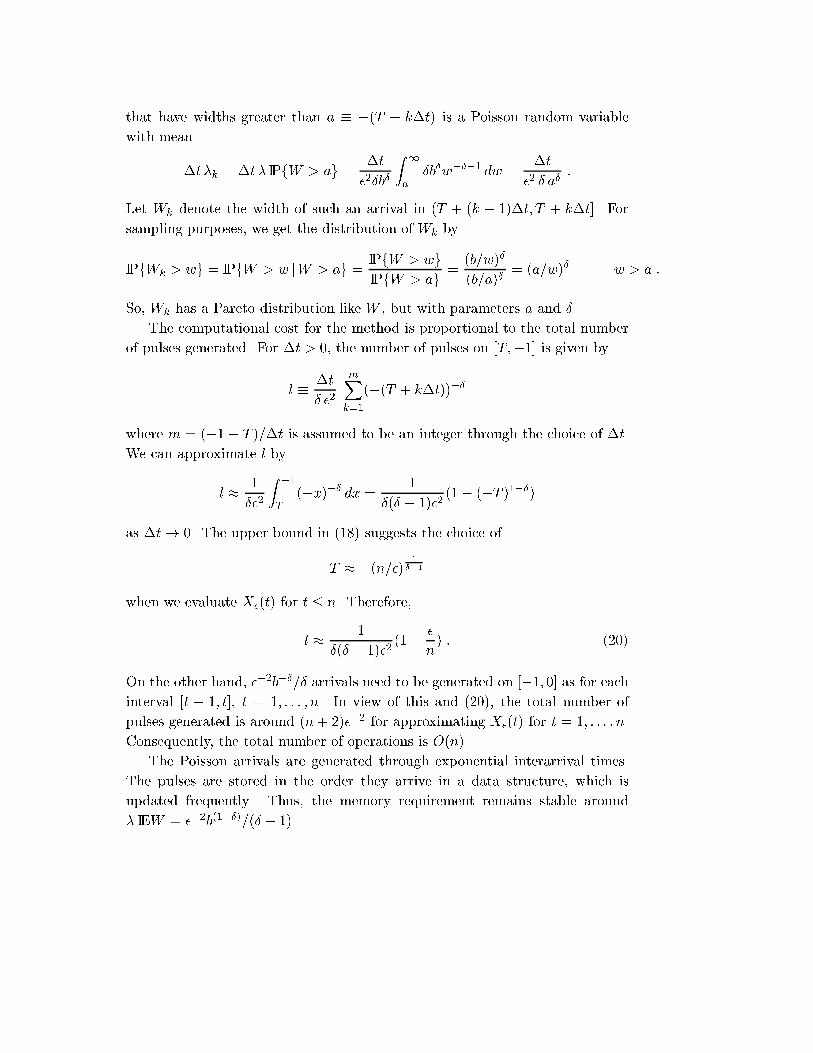
The computational cost for the method is proportional to the total number

of pulses generated. For �t > 0, the number of pulses on [T;�1] is given by

l � �t

� �2

mXk=1

(�(T + k�t))��

where m = (�1� T )=�t is assumed to be an integer through the choice of �t.

We can approximate l by

l � 1

��2

Z �1

T(�x)�� dx =

1

�(� � 1)�2(1� (�T )1��)

as �t! 0. The upper bound in (18) suggests the choice of

T � �(n=�) 1

��1

when we evaluate X�(t) for t � n. Therefore,

l � 1

�(� � 1)�2(1� �

n) : (20)

On the other hand, ��2b��=� arrivals need to be generated on [�1; 0] as for eachinterval [t � 1; t], t = 1; : : : ; n. In view of this and (20), the total number of

pulses generated is around (n+ 2)��2 for approximating X�(t) for t = 1; : : : ; n.

Consequently, the total number of operations is O(n).

The Poisson arrivals are generated through exponential interarrival times.

The pulses are stored in the order they arrive in a data structure, which is

updated frequently. Thus, the memory requirement remains stable around

� IEW = ��2b(1��)=(� � 1).

Suppose the desired variance parameter of FBM is � > 0, that is,

Cov(X(t1);X(t2)) =�

2(t3��1 + t3��2 � jt1 � t2j3��) :

Then, the steps to get X�(t) for t = 1; : : : ; n, with n � (�T )��1, are as fol-

lows.

1. Input 0 < � < 1, 1 < � < 3 (� = 3 � 2H), and 0 < b < 1. Compute

x =p�=c.

2. Let T0 = T < T1 < T2 < : : : < TK = 0 be a mesh of [T; 0]. In each interval

[Tk�1; Tk], k = 1; : : : ;K, generate Poisson arrivals with rate

�k =1

�2�(�Tk)� :

Associate widths wi from the Pareto density (12) with cuto� b = �Tk.Repeat Step 3 for t = 0; 1; : : : ; n.

3. Compute Y�(t) by (19). Generate Poisson arrivals on [t; t + 1] with rate

� = ��2b��=�. Associate widths from the Pareto density (12). Update

the stack of pulses by adding the new arrivals and deleting the pulses that

have �i + wi < t+ 1.

4. X�(t) = Y�(t)� Y�(0), t = 1; : : : ; n.

5 Simulations

In this section, we �rst display sample traces of FBM. Then, several traces are

simulated for statistical con�rmation of the accuracy of the method with wavelet

estimation. In particular, the estimator of the peakedness parameter is studied

empirically.

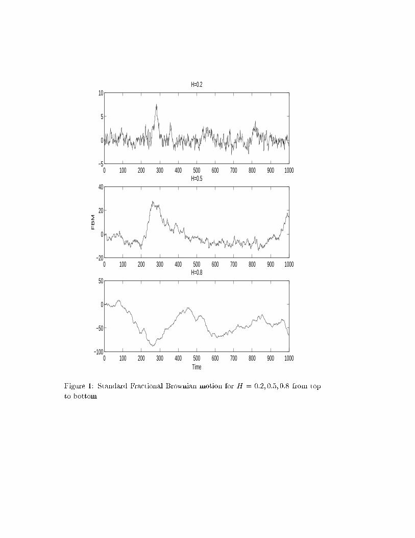
Fractional Brownian motions for H = 0:2; 0:5; 0:8 are plotted in Figure 1 for

t = 0; 1; 2; : : : ; 1000. The value of T is �105 for H = 0:2; 0:5, and �1010 for

H = 0:8. The value of � is 0:1, which ensures that su�ciently many pulses are

aggregated to achieve a Gaussian distribution. The variance � is chosen to be 1,

and the value of b is such that �b� = 1 which yields 0 < b < 1. The corresponding

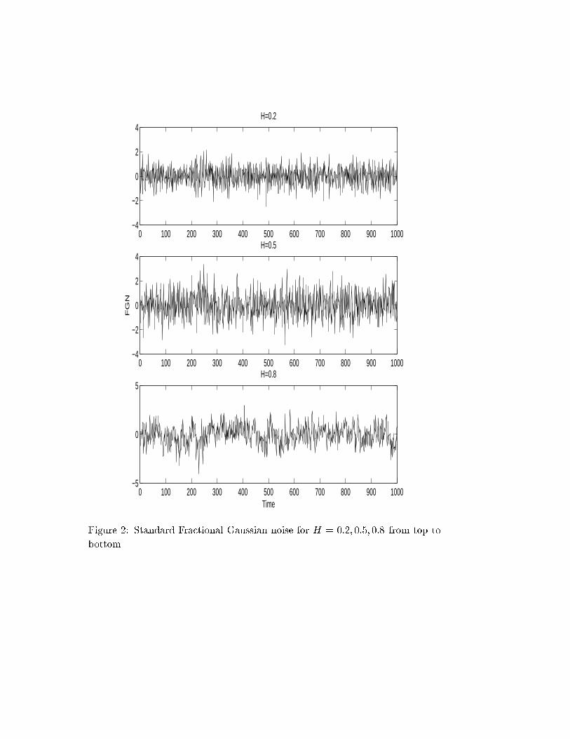
fractional Gaussian noises are given in Figure 2 for t = 1; 2; : : : ; 1000. The e�ect

0 100 200 300 400 500 600 700 800 900 1000−5

0

5

10H=0.2

0 100 200 300 400 500 600 700 800 900 1000−20

0

20

40H=0.5

FB

M

0 100 200 300 400 500 600 700 800 900 1000−100

−50

0

50H=0.8

Time

Figure 1: Standard Fractional Brownian motion for H = 0:2; 0:5; 0:8 from top

to bottom.

0 100 200 300 400 500 600 700 800 900 1000−4

−2

0

2

4H=0.2

0 100 200 300 400 500 600 700 800 900 1000−4

−2

0

2

4H=0.5

FG

N

0 100 200 300 400 500 600 700 800 900 1000−5

0

5H=0.8

Time

Figure 2: Standard Fractional Gaussian noise for H = 0:2; 0:5; 0:8 from top to

bottom.

of b < 1 on the error of the variance � is small as we plot for t greater than or

equal to 1.

It is well known that the qualitative di�erence between these graphs comes

from the sign of the autocorrelation of the increments of FBM X in nonoverlap-

ping intervals. We have, for each h > 0,

Cov(X(t+h)�X(t);X(t)�X(0)) = IE [X(t)(X(t+h)�X(t))] =1

2[(t+h)2H�t2H�h2H ]

which is positive forH > 1=2, negative forH < 1=2, and is zero forH = 1=2, cor-

responding to the persistent, antipersistent and independent cases, respectively.

Indeed, the plots of FGN uctuate less as H increases, which is consistent also

with the FBM plots. For example for H = 0:8 in Figure 1, the process is inclined

to increase (decrease) if it has already increased (decreased) in the previous in-

terval. The rightness of the choice of �, b and T can be checked from FGN plots

qualitatively. Since these plots are over unit intervals, we are plotting Gaussian

random variables with mean 0 and standard deviation 1 in all cases. Clearly,

the di�erences are due to those of the autocorrelations.

To test the accuracy of the simulation procedure, we estimate the param-

eters H � (3 � �)=2 and � � cx2 of (8) jointly by the wavelet estimation

method of veitch and abry (1997). This method has proven to be quite pre-

cise for estimating the Hurst parameter; see for example fischer and akay

(1996), and mehrabi et.al. (1997) among others. The work of veitch and

abry (1997) takes it one step further by jointly estimating a form of the scale

parameter as well as the shape parameter in long-range dependent processes.

The shape parameter they consider is a linear function of H in our case. The

scale parameter they consider is denoted by cf , which is the coe�cient in

f(�) � cf j�j�(2H�1) � ! 0

where f is the spectrum of the stationary long-range dependent process, in our

case FGN. Because of long-range dependence, their analysis refers to H > 1=2

for FGN, however it can be extended to H � 1=2 without loss of generality.

In the FBM tra�c model of (1), we have

A(t) = mt+pmaX 0(t) (21)

where X 0 is a normalized FBM with � = 1. In the simulated traces of this

section, we have also set � = 1. However, we treat � as an unknown in the

estimation process. Then one could take

X(t) � pmaX 0(t)

and hence

V ar(X(t)) = �t2H = ma t2H = maV ar(X 0(t)) = V ar(A(t))

Then, estimating � from a trace of X is equivalent to estimating \ma" from a

trace of A as they are both the variance coe�cients. This is in turn eqivalent

to estimating the peakedness parameter a by a = �=m once the mean m is

estimated. That is why, we estimate � to illustrate the estimation of a in (21)

rather than cf , as a directly appears in the tra�c model, while cf does not.

Besides, when the micropulses algorithm is used for simulation of FBM, the

input parameter is � not cf . Then, the parameter � is given in terms of cf by

� =cf (2�)

2H�1

2�(2H � 1) cos((2H � 1)�=2)(2H � 1)HH 6= 1

2: (22)

In the estimation process, there are two unbiased estimators, namely, those

of H and cfC where C is the integral

C =

Zj�j�(2H�1) j0(�)j2 d� (23)

of the Fourier transform 0 of the mother wavelet. In particular, we use

Daubechies wavelets with two vanishing moments. Under mild assumptions,

which approximately hold in the case of FGN, the estimators H and dcfC are

both unbiased. Essentially, we estimate � through (22) using the estimators

cf and H where cf = dcfC=C and C is the integral (23) computed with H.

However, being an involved function of these estimators � is not necessarily un-

biased. It can be interpreted as the variance per time lag that the observations

are separated, which is usually taken as the unit time 1. When the estimation

is desired for another time unit, say times the time unit of the observations,

the estimator � must be written in full generality as

� =cf (2�)

2H�1 2H

2�(2H � 1) cos((2H � 1)�=2)(2H � 1)H: (24)

This follows by the fact that V (Xt+ �Xt) = �1 2H where �1 = V (Xt+1 �Xt)

is the variance per the time unit of the observations.

For particular simulations in veitch and abry (1997), H and cf perform well

especially with samples of length at least 212. We have simulated 100 samples

of FGN for each H = 0:1; 0:2; : : : ; 0:9, by setting � = 1. In the preliminary

trials, FGN was generated for 213 time units, and b was such that �b� = 1 so

that the arrival rate was just ��2. This produced 0 < b < 1 for all 1 < � < 3

justifying the sampling at unit intervals. Here, the variance of � appeared to be

large for H < 1=2 although its bias was in an acceptable range. Decreasing b

improved the results in view of Section 4.1. So, for H � 1=2, we choose b = 0:3,

sample twice in each time unit for n = 212, yielding a sample size of 213 in

the estimation stage. For H > 1=2, b is such that �b� = 1, and n = 213. The

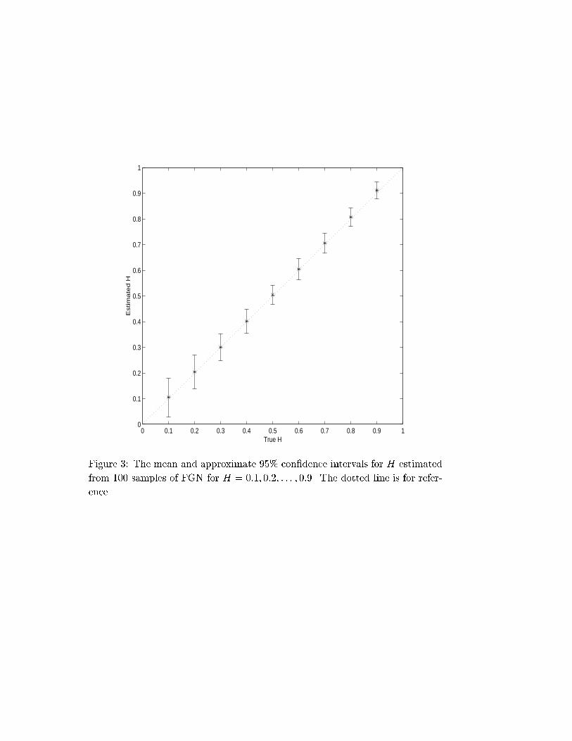
mean of the estimators of H as well as the approximate 95% con�dence intervals

are given in Figure 3. Since the estimator of H is unbiased theoretically, the

results indicate that the aggregation method is accurate in terms of the shape

parameter H. The means and con�dence intervals for � are given in Figure 4.

In view of the time units, � is found by setting = 1 for H > 1=2 and = 2 for

H � 1=2 in (24). From Figure 4, we see that the estimator � is either biased or

the aggregation method produces samples of larger variance than we intended.

To reach a conclusion, we have also estimated dcfC, which is known to be

unbiased. The true values of cf are found by the equation

cf =2��(2H � 1) cos((2H � 1)�=2)(2H � 1)H

(2�)2H�1 2HH 6= 1

2

which takes the desired time unit into account through . This consideration

is done in the true value rather than cf , not to upset the unbiasedness of the

estimator. For H = 1=2, f(�) = cf is a constant. Since the time unit is 0.5

for H = 1=2, we have cf = V (Xt+0:5 � Xt) = 0:5 and cfC = 0:5 as C = 1.

The con�dence intervals on the estimator are found by normal approximation

because this gives almost the same result as the lognormal distribution, which

is the approximate distribution of dcfC. The true and estimated values of cfC

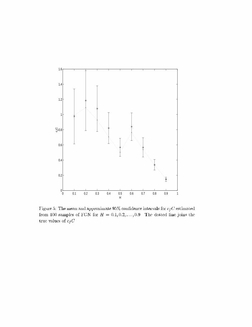
together with approximate 95% con�dence intervals are given in Figure 5. We

see that for some H, dcfC is very close to cfC, and for others there is some error.

Since the aggregation method is exactly the same for all H, the di�erence is due

to the randomness in simulation. The bias is at most 20%, which we expect

to decrease for longer samples. The variances, on the other hand, are directly

proportional to the magnitude of cfC, which is as expected from the theoretical

variance given in veitch and abry (1997). Therefore, the aggregation method

with micropulses is accurate in terms of the scale parameter as well.

0 0.1 0.2 0.3 0.4 0.5 0.6 0.7 0.8 0.9 10

0.1

0.2

0.3

0.4

0.5

0.6

0.7

0.8

0.9

1

Estim

ate

d H

True H

Figure 3: The mean and approximate 95% con�dence intervals for H estimated

from 100 samples of FGN for H = 0:1; 0:2; : : : ; 0:9. The dotted line is for refer-

ence.

0 0.1 0.2 0.3 0.4 0.5 0.6 0.7 0.8 0.9 10

0.5

1

1.5

2

2.5

Estim

ate

d α

H

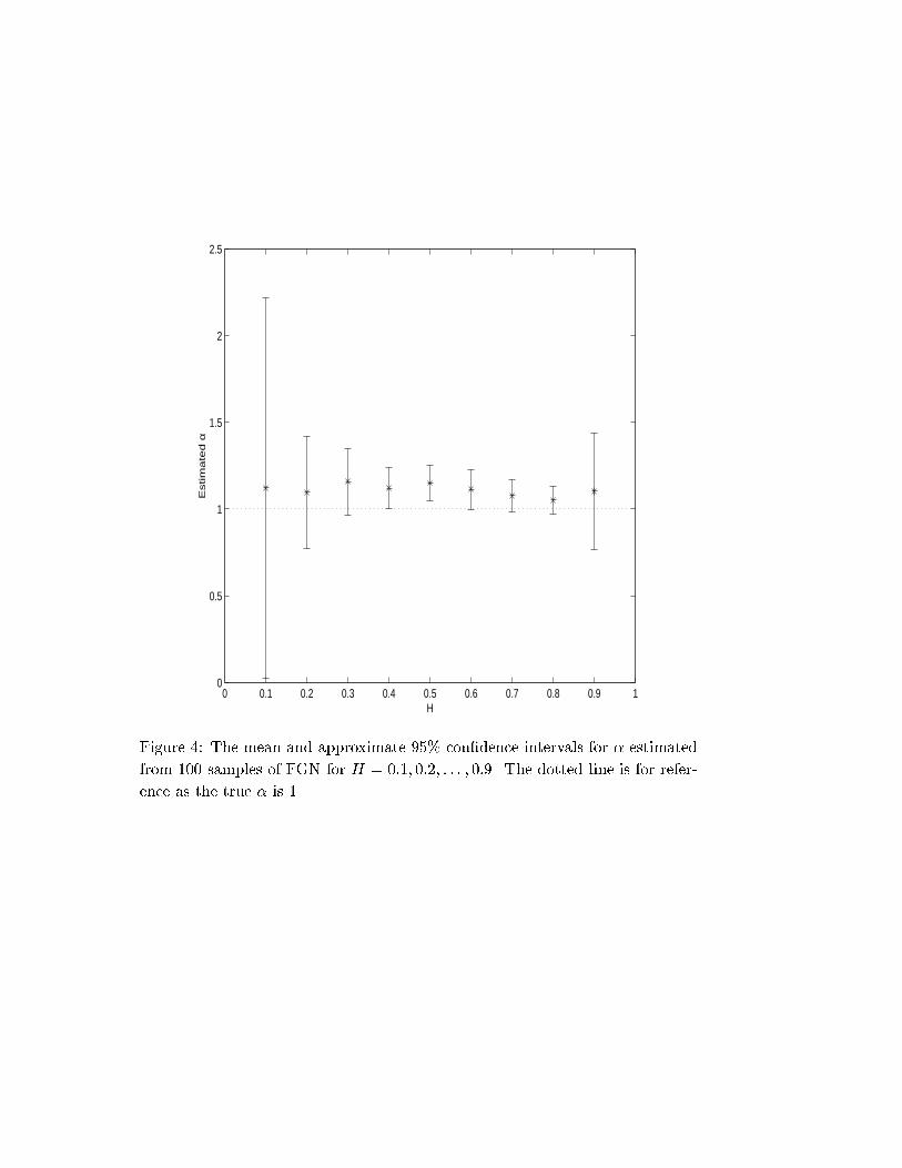
Figure 4: The mean and approximate 95% con�dence intervals for � estimated

from 100 samples of FGN for H = 0:1; 0:2; : : : ; 0:9. The dotted line is for refer-

ence as the true � is 1.

Finally, with con�dence in the aggregation method with micropulses, we can

interpret Figure 4 from estimation aspect. The variance of � is huge for small

H somewhat in accordance with that of the corresponding cfC. It is larger than

expected for small H and also for H = 0:9. The estimator � could be slightly

biased as it deviates from the true value, which is not even in the con�dence

interval for some H in our simulations. However, the error being less than

20% as in the unbiased estimator dcfC, with moderate variances for H > 1=2,

this method of estimation of � would be useful for long-range dependence in

telecommunication studies.

Acknowledgement. I would like to thank Dr. Iraj Saniee for introducing me

to the tra�c models with fractional Brownian motion. This work would not

have been possible without his invaluable suggestions and comments.

REFERENCES

P. Abry and F. Sellan (1996) The Wavelet-Based Synthesis for Fractional

Brownian Motion Proposed by F. Sellan and Y. Meyer: Remarks and Fast

Implementation. Appl. Comp. Harmonic Anal. 3: 377-383.

J. Beran et.al. (1995) Long-Range Dependence in Variable-Bit-Rate Video

Tra�c. IEEE Trans. on Commun. 43: 1566-1579.

R. Cioczek-Georges and B.B. Mandelbrot (1995) A Class of Micropulses

and Antipersistent Fractional Brownian Motion. Stoch. Proc. Appl. 60: 1-18.

R. Cioczek-Georges and B.B. Mandelbrot (1996) Alternative Micropulses

and Fractional Brownian Motion. Stoch. Proc. Appl. 64: 143-152.

M. Crovella and A. Bestavros (1996) Self-Similarity in World Wide Web

Tra�c-Evidence and Possible Causes. Proceedings of ACM Sigmetrics '96.

Philadelphia, PA, 160-169.

D.E. Duffy et.al. (1994) Statistical Analysis of CCSN/SS7 Tra�c Data from

Working Subnetworks. IEEE J. Select. Areas Commun. 12: 544-551.

A. Erramilli et.al. (1996) Experimental Queuing Analysis with Long-Range

Dependent Packet Tra�c. IEEE/ACM Trans. On Networking 4(2) : 209-223.

R. Fischer and M. Akay (1996) A Comparison of Analytical Methods for the

Study of Fractional Brownian Motion. Annals of Biomedical Engineering 24:

537-543.

0 0.1 0.2 0.3 0.4 0.5 0.6 0.7 0.8 0.9 10

0.2

0.4

0.6

0.8

1

1.2

1.4

1.6

cfC

H

Figure 5: The mean and approximate 95% con�dence intervals for cfC estimated

from 100 samples of FGN for H = 0:1; 0:2; : : : ; 0:9. The dotted line joins the

true values of cfC.

H.J. Fowler andW.E. Leland (1991) Local Area Network Tra�c Character-

istic, with Implications for Broadband Network Congestion Management. IEEE

J. Select. Areas Commun. 9: 1139-1149.

D. Heath et.al. (1998) Heavy Tails and Long Range Dependence in On/O�

Processes and Associated Fluid Models. Mathematics of Operations Research

23: 145-165.

W.E. Leland et.al. (1994) On the Self-Similar Nature of Ethernet Tra�c

(extended version). IEEE/ACM Trans. on Networking 2: 1-15.

W-C. Lau et.al. (1995) Self-Similar Tra�c Generation: The Random Midpoint

Displacement Algorithm and its Properties. IEEE International Conference on

Communications. 1: 466-472.

B.B. Mandelbrot and J.W. Van Ness (1968) Fractional Brownian Motions,

Fractional Noises and Applications. SIAM Review 10: 422-437.

B.B. Mandelbrot and J.R. Wallis (1969) Computer Experiments with Frac-

tional Gaussian Noises. Water Resources Research 5: 228-267.

A.R. Mehrabi, H. Rassamdana and M. Sahimi (1997) Characterization of

Long-Range Correlations in Complex Distributions and Pro�les. Physical Re-

view E 56: 712-722.

K. Meier-Hellstern et.al. (1991) Tra�c Models for ISDN Data Users: O�ce

Automation Application. Proc. 13th ITC. Denmark, 167-172.

I. Norros (1995) On the Use of Fractional Brownian Motion in the Theory of

Connectionless Networks. IEEE Jour. Selec. Areas in Comm. 13: 953-62.

V. Paxon and S. Floyd (1995) Wide-Area Tra�c: The Failure of Poisson

Modeling. IEEE/ACM Trans. on Networking 3(3): 226-244.

V. Paxon (1997) Fast, Approximate Synthesis of Fractional Gaussian Noise

for Generating Self-Similar Network Tra�c. Computer Communication Review

27(5): 5-18.

G. Samorodnitsky and M.S. Taqqu (1994) Stable Non-Gaussian Random

Processes. Chapman & Hall. New York, NY.

F. Sellan (1995) Synth�ese de Mouvements Browniens Fractionaires �a l'aide de

la Transformation par Ondelettes. C. R. Acad. Sci. Paris S�er. I Math. 321:

351-358.

M.S. Taqqu,W. Willinger and R. Sherman (1997) Proof of a Fundamental

Result in Self-Similar Tra�c Modeling. Computer Communication Review 27:

5-23.

G. Wornell (1990) A Karhunen-Lo�eve like Expansion for 1/f Processes via

Wavelets. IEEE Trans. Inform. Theory 36: 859-861.

D. Veitch and P. Abry (1997) A Wavelet Based Joint Estimator of the Pa-

rameters of Long-Range Dependence. Submitted to special issue \Multiscale

Statistical Signal Analysis and its Applications" IEEE Trans. Info. Th.

Z.-M. Yin (1996) New Methods for Simulation of Fractional Brownian Motion.

Jour. of Comp. Phys. 127: 66-72.