simulation of gravitational waves and binary black...
TRANSCRIPT

Simulation of Gravitational Waves and Binary BlackHoles Space-times
Master's Thesis in Masters Degree Programme, Radio and Space Science
FAHAD NASIR
Department of Fundamental PhysicsCHALMERS UNIVERSITY OF TECHNOLOGYGöteborg, Sweden 2010.

The Author grants to Chalmers University of Technology and University of Gothenburgthe non-exclusive right to publish the Work electronically and in a non-commercialpurpose make it accessible on the Internet. The Author warrants that he/she is the authorto the Work, and warrants that the Work does not contain text, pictures or other materialthat violates copyright law.The Author shall, when transferring the rights of the Work to a third party (for example apublisher or a company), acknowledge the third party about this agreement. If the Authorhas signed a copyright agreement with a third party regarding the Work, the Authorwarrants hereby that he/she has obtained any necessary permission from this third party tolet Chalmers University of Technology and University of Gothenburg store the Workelectronically and make it accessible on the Internet.
Simulation of Gravitational Waves and Binary Black Holes Space-timesOverview of Gravitational Wave Science. Extraction of Gravitational Waves with post-Newtonian Approximation and Numerical Relativity Formulation
FAHAD NASIR,
© FAHAD, NASIR, January 2010
Examiner: Martin Cederwall
Department of Fundamental PhysicsChalmers University of TechnologySE-412 96 GöteborgSwedenTelephone + 46 (0)31-772 1000

Department of Fundamental PhysicsGöteborg, Sweden January 2010

Simulation of Gravitational Waves and Binary Black Holes Space-times
Fahad Nasir
Department of Fundamental PhysicsChalmers University of Technology
Abstract
The main objective of this thesis is to study gravitational radiation along with its associatedphenomena, specifically for binary black holes. The occurrence of such events in our universehave profound implications when gravitational waves are radiated by accelerating massiveastrophysical bodies. The specific system under our consideration is a binary black hole. Thetwo essential phases of binary black hole, namely inspiral and merger have their characteristicgravitational wave signature. Gravitational waves during these phases are obtained by takingadvantage of powerful numerical tools available. Two popular techniques are applied todetermine waveforms, namely post-Newtonian approximation for the inspiral phase andnumerical relativity techniques for the merger phase of binaries. The nature of gravitational wave is explained by considering the linearised theory of generalrelativity and its effect on free-falling bodies. A detailed description of the multipoleexpansion is provided which also encompasses the famous Einstein quadrupole formula. Forthe inspiral phase of binary black holes, the post-Newtonian formalism is discussed in detail.Extraction of waveforms by the post-Newtonian method is implemented by MATLABroutines to test the findings. Lastly, the foundation of numerical relativity is reviewed whichserves the purpose to carry out further discussions on gravitational waves in strong gravityregime during merger phase of binaries. ADM and BSSN formalism is introduced along withthe Schwarzschild and Misner initial data. BSSN evolution of Misner initial data is carried outby CCATIE code. The Weyl scalars are extracted to provide an invariant way of representingoutgoing gravity waves at various stages of evolution.
4

Acknowledgements
I express my gratitude to my supervisor, Martin Cederwall for his kind help and support.Without his exhilaration and encouragement this work would not have been possible. Thediscussions proved to be really conducive and kept me motivated throughout the whole thesiswork. I am grateful to the department of Fundamental Physics for providing me theopportunity. I am thankful to the department of Radio and Space for providing the necessarytheoretical foundation which made all this effort conceivable. Special thanks to John H. Blackfor introducing me to our strange universe of black holes and quasars . Finally, I be indebtedto my room-mates, Hassan and Junaid, for such refreshing discussions during stress times.
5

Contents1 Introduction.....................................................................................................................6 Outline...............................................................................................................................8
2 Gravitational Wave Sources...........................................................................................92.1 Binary Black Hole Mergers..........................................................................................102.3 Neutron Star and Black Hole Mergers.........................................................................102.4 Neutron Star and Neutron Star Inspiral........................................................................112.6 Neutron Star Birth........................................................................................................112.7 Gravitational Waves from Early Universe...................................................................12
3 Gravitational Radiation................................................................................................133.1 Short Wave Approximation..........................................................................................133.2 Equation of Geodesic Deviation...................................................................................143.3 Mathematical Description of Gravitational Wave........................................................153.4 Linearised Einstein's Equations....................................................................................173.5 Multipole Moments Decomposition.............................................................................203.6 Expansion in Source Region for Slow Motion Sources...............................................23
4 Post-Newtonian Approximation ..................................................................................264.1 Post-Newtonian Approximation...................................................................................264.2 TaylorT2.......................................................................................................................284.3 TaylorT3........................................................................................................................294.5 Extraction of Waveform by Stationary Phase Approximation.....................................31
5 Numerical Relativity.....................................................................................................345.1 Arnowitt-Deser-Misner (ADM) Formulation .............................................................355.2 Baumgarte-Shapiro-Shibata-Nakamura (BSSN) Formulation.....................................375.3 Boundary Conditions ...................................................................................................395.4 Gauge Conditions.........................................................................................................405.5 Initial Data for Black Hole ..........................................................................................415.5.1 Schwarzschild Initial Data.........................................................................................415.5.2 Misner Initial Data.....................................................................................................425.6 Results and Discussion.................................................................................................435.6.1 Schwarzschild Initial Data Evolution........................................................................435.6.2 Misner Initial Data Evolution....................................................................................46
6 Conclusion and Future Work.......................................................................................52References............................................................................................................................53
7 Appendix........................................................................................................................55A.1 Compiling and Running Cactus Framework ..............................................................55A.2 Cactus Parameters Files...............................................................................................61A.3 Simulation of Binary Inspiral - MATLAB Code.........................................................65
6

1 Introduction
General relativity was formulated by Einstein on the foundation of the equivalence principle.Gravity waves travelling at speed of light is an inevitable consequence of such a principle. Agravitational wave (GW) can be regarded as a fluctuation in space-time which travel outwardscarrying energy from source. Such ripples in space-time are the result of complex dynamics ofmassive dense objects or due to the interaction of massive stars, black holes or neutron starsbinaries. Once produced, they can travel unhindered straight to the earth without muchinteraction with the matter. Such disturbance appear as distorted space-time to a distantobserver. However our earth is minuscule compare to the wavelength of GW, as distances areso tremendous that their detection is huge challenge posed by modern astronomy.
After Einstein had formulated his theory of general relativity, within months he figured outthe famous quadrupole formula for gravitational waves, which is valid for bodies withnegligible self-gravity. Till mid 1920s, linearised theory was understood due to thecontributions by Weyl (1922) and Eddington (1924). Landau and Lifshitz gave the firsttheoretical treatment of radiation emission by self-gravitating bodies [2]. However in 1940'sand 1950's, scientific community was not considering GW as a physical possibility to carryenergy from the system. Feynman proposed “Sticky Bead” thought experiment to prove theexistence of such waves carries energy. The thought experiment states that any passing waveshould move any bead on stick back and froth, hence producing friction and thus concludingthat wave carries energy. Later on Bondi, Weber and Wheeler developed the formalism basedon Feynman argument. Bar detectors were build around the world to detect waves fromvarious astrophysical sources. The effort was initiated by Weber which eventually detectedelectrical signals at two bar detectors ( one at chicago and other near Washington DC)simultaneously. In 1970s, soviet scientist suggested to develop Michelson-Morleyinterferometers for detection of gravitational waves. In 1973, a major breakthrough happened,when Taylor and Russell Hulse detected pulsar 1913+16 which was in a binary. The orbitaldecay (76.5 ms per year) was precisely consistent with the energy carried away by the wavesas predicted by general relativity. In 2003, another major binary pulsar J0737-3039 wasdiscovered, which also agrees well with predictions of general relativity. The technologicalefforts made in 70's contributed to the second generation of detectors with advanced coolingtechniques. Several interferometers are now operating around the world like LIGO, GEO,VIRGO and TAMA. The bursts sensitivity now has reached Khz ( h~10−17 ) increasing thepossibility of detecting such an event to about 3/yr. The sensitivity of detectors can be dividedinto high ( f ≥10 Hz ), low (10−5 Hz≤ f ≤10 Hz) and extremely low ( f ≤10−5 Hz ) frequencybands. For detailed discussion on history of gravitational wave research, see [2,22,25].
Gravitational waves provide a possible way to probe the distant universe and test exotictheories related to cosmology, the early universe and extreme gravitational regimes. Thedifferences mentioned in table 1.1. mark gravitational waves astronomy as revolutionary andwill potentially have much more profound impact as compared to radio waves astronomy.However we know that the electromagnetic astronomy is mature and well established field sothe promises seem blown out of proportion. The possible reason for this is that sourcedistances or strengths are uncertain with several orders of magnitude, with the exception ofbinaries.
7

In the future, possible detection of GW may give us extensive information about the universeand make it possible to test physical laws which can never be tested by any other methodknown to date. When gravitational waves and light arrive to earth from a astrophysical sourceit should confirm the prediction of general relativity that the light and gravity waves bothtravels with same speed. The polarisation of gravitational waves may confirm that thegravitons are transverse traceless and gravitons have spin 2.
The primary purpose of simulating the binaries and supernovae bursts is to extract waveformsand compare them with the ones obtained from the actual sources which can eventuallyconfirm the dynamics of the system predicted by general relativity. This will not only provethe existence of black holes but provide ample clue for determining various physical featuresof the system. Moreover, GW astronomy can offer a very strict test to general relativity instrong gravitational field.
The greatest challenge with such simulations is to extract waveforms to an accuracy whichcan be matched filtered with the noisy waveform received. Matched filtering with a bank ofwaveforms results in identifying and estimating the various parameters in the dynamics of thesource. Post-Newtonian approximations are popular to produce waveform banks when propernumerical tools are incorporated [24].
An even great challenge is to simulate the extreme space-time around binaries when post-Newtonian approximations are not anymore accurate. In such situations Baumgarte-Shapiro-Shibata-Nakamura (BSSN) formalism of Einstein's equations proved to provide stablesimulations with constrained evolutions [1,15,16,17].
Table 1.1. The comparison between for electromagnetic and gravitational wavesElectromagnetic Waves Gravitational WavesAccelerating charges produce time changingdipole moments
Incoherent superposition of radiation fromelectrons, atoms, and molecules
Information about the thermodynamics of thesystem
Wavelength small compared to the source
Scattered, absorbed by the matter
Very high frequency ranges (observationfrequencies at KHz and MHz)
Accelerating masses produce time changingquadrupole moments
Coherent superposition of radiation from thehuge dense mass source like black hole andmassive stars
Direct information about the dynamics of thesystem
Wavelength are large compared to the source
Negligible interaction with the matter
Very low frequency range (frequencies rangeis several orders less then 10Hz)
8

Outline
In chapter 2, a very quick review of gravitational wave sources is given. We have tried topossibly list all the primary GW sources with their brief description. Description of how GWare studied in various bandwidth, provide profound information about universe.
Chapter 3 is the very foundation of gravitational radiation. Basic concepts are discussed andformalism is introduced. The very nature of GW is explored by linearised general relativity.The multipole decomposition of field is the key concept developed in this chapter.
In chapter 4, we starts with a description of post-Newtonian approximation with all itslimitations and applications. The post-Newtonian expressions are being implemented byMATLAB routines and results are discussed.
The last chapter is a precise description of topics concerning numerical relativity. Theessential formulations are introduced which are crucial for binary evolution problem.Schwarzschild and Misner initial data are discussed and the results for their evolution arepresented.
9

2 Gravitational Wave Sources
Theoretically, any mass that accelerates is a source of gravitational waves. From anaccelerating meteoroid in an orbit around sun to inspiralling black holes or even explodingsupernovae, all are sources of radiation. Unfortunately the strengths of such sources are muchweaker, or when the wave reaches earth its become painfully feeble, making extremelychallenging to detect. The sources vary from binaries to the supernovae bursts where eachphenomenon has its own characteristic GW, giving clues about the dynamics of the system.The most common type of dynamics we deal with is of binaries. To describe a simple binarysystem, one assumes two huge astrophysical objects which orbit around some centre of masswhich depends on magnitude of two masses (in the centre, for equal size binary). Such massescan be neutron stars or even black holes. However, stars like our sun generate radiation atsuch a small scale that its detectability is impossible with our present technology or even innear future. When binaries inspiral they move deep into a potential well giving its excessenergy in form of radiation. The orbit become smaller and smaller, eventually this downwardinspiral results in coalescence of the two bodies. When the binary become effectively onebody its rotation of non-spherical shape also results in GW. Now, we will briefly discuss someof the wave sources with all their associated phenomena.
Figure 2.1. Various frequency bands in GW astronomy are shown along with the mechanismcausing the radiation. Universe phase transitions, cosmic strings and domain walls are someof the exciting futuristic subjects which can be studied by radiation. GW emission from binaryblack holes and neutron stars are studied at low frequencies and high frequencies bands whichis of principle interest in our work.
10

2.1 Binary Black Hole Mergers
Stellar mass black holes exist in galaxies and globular clusters (stars clusters orbiting ingalactic core). Supermassive black holes can form at galactic nuclei due to the merger ofgalaxies. The inspiral and merger of black hole is strange and extremely interesting toobserve. Such mergers are one of the spectacular sources of radiation. The black holes areextremely dense objects, thus results in much less coalescence time and a lot of fascinatingradiation. Stellar mass black holes emit GW in the high frequency band and have been probedby Laser Interferometer Gravitational Observatory (LIGO), while waves in the low frequencyband will be studied by Laser Interferometer Space Antenna (LISA) [27]. The informationprovided by binary black hole waveforms is profound. The surface areas, masses, spins, orbitsin curved space-time and nonlinear dynamics, can all be established from the waveformsignature. Moreover, we can test the Penrose cosmic censorship conjecture, the second law ofblack hole mechanics and how they pulsate and lose their excess hair by radiation.Gravitational waveforms can be extracted by various methods in different phases of thebinaries. Inspiral phase waveforms can be extracted by post-Newtonian approximation,merger by numerical relativity and finally ring-down by perturbation theory.
Table 2.1. Showing the equipment designed for GW observation, the distance they are able toprobed along with their respective signal to noise ratios (SNR) for binaries [27].Equipment Distance Event Rate SNRLIGO and InitialInterferometers
100 Mpc 1/200 yr to 1/yr 10 or less
LIGO and AdvancedInterferometers
z~0.4 2/month to 15/day 10 to 100
LISA z~10 few/yr 100 to 100,000
2.2 Neutron Star or Small Black Hole Inspiral into Supermassive Black Hole
Supermassive black holes are mostly located at the galactic nuclei. Occasionally small blackholes and neutron stars inspiral and finally plunge into such supermassive black holesresulting in a myriad of radiation. The rate of such events are about few per year to thedistances probe by LISA. Such GW waveform probe into galactic nuclei and supermassiveblack hole space-time. Waves are emitted in the low frequency spectrum. Mapping black hole,evolution of horizons and test of no hair theorem are one of the exotic conjectures which canbe tested with such data. Black hole perturbation theory is the key framework for obtainingsuch waveforms.
2.3 Neutron Star and Black Hole Mergers
The existence of such events can be found in globular clusters. Initially the neutron star andthe black hole go into a downward inspiral, and eventually the neutron star forms lobes whichare sucked into black hole. GW emitted usually lies in the high frequency band. Initialinterferometers have probed to 43 Mpc with event rate 1 /2500 yr−1/ 2 yr. Advancedinterferometers rates can quest up to at 650 Mpc with occurrence rate 1 / yr−4 /day.
11

Waves convey information about the spin, orbit, masses, tidal disruption of neutron star andits structure. Theories about neutron star evolution and its equation of state for matter can betested and verified. Both post-Newtonian and numerical relativity techniques are employed toobtain waveforms depending on the phase of binaries.
2.4 Neutron Star and Neutron Star Inspiral
Such events can happen when main sequence progenitors in the galaxy capture binaries inglobular clusters. Waves are emanated in the high frequency band. Initial interferometers havestudied distances up to 200 Mpc with rates 1/3 yr-1 - 1/300 yr-1 while advanced interferometersup to 300Mpc with rates 1/yr - 3/day. Information carried by waveform is about masses,spins, and orbit during inspiral phase. But during merger phase information is lost due to highnoise of equipment. Relativistic effects can be studied during inspiral phase. The method forextraction of waveforms is post-Newtonian approximation.
2.5 Spinning Neutron Stars or Pulsars
Spinning neutron stars are known as pulsars and lie the in high frequency band of thespectrum. Pulsar rotation rates are found to be ~ 250-700 rev/s. The mountains on the surfaceof neutron stars cause emission of radiation, which tries to reduce the spin of star. However,spin rates are kept in this limit when radiation torque is in balance with the accretion disctorque around neutron star. In such steady state, X-ray luminosity (due to rate of accretion ofmass around neutron star) is proportional to wave strength. Detectability of the star dependson the spin and ellipticity of the pulsating neutron star. Pulsar ellipticity is generally of order≤10−6. Ellipticity also decides the frequency of pulsars. GW helps probing neutron starstructure and its behaviour during birth. Slow motion and strong gravity techniques are usedfor analysis of the problem. Both X-ray luminosity and GW yield information about thetemperature, crust and viscosity of the neutron star.
2.6 Neutron Star Birth
Neutron stars can be formed due to supernovae explosions or due to the collapse of accretioninduce white dwarf. R-mode (radial modes of vibration) instability depends on the spin of theneutron star. If period of spin is less then 10-3 s, then neutron star is R-mode unstable.Moreover the GW emission drives the R-mode sloshing. We still don't have evidence whatstops the growth of sloshing at later stages. GW give us insight about crust formation,coupling of R-modes, wave breaking, shock formation and magnetic field torques. Any ofthese can be the reason of stopping sloshing growth.
Figure 2.2. R sloshing of spinning neutron star causes emission of GW
12
2.7 Gravitational Waves from Early Universe
Gravitational waves were originated even during the big bang, but the expansion of universered-shifted the waves. Inflation results in amplification of quantum fluctuations which leadsto primordial GW. As time progresses the fundamental forces of universe decoupled, causingphase transitions, which again produce GW. Electroweak phase transition ( ~100 GeV)occurred when universe was about 10-11 s old. LISA can probe to electroweak phase transition,while LIGO can probe to phase transition which has occurred at ~109 GeV or when age ofuniverse was ~10-25 s old. Waves in all bands provide information about early universe phases.Inflation can be studied by cosmic microwave background anisotropy at extremely lowfrequencies. GW can inquest into physics of big bang, inflation and equation of state of verythe primitive universe. Quantum gravity and cosmological perturbation theory can assist thestudy and analysis of waveforms. Such studies can help to determine strength of electroweakphase transition, and to probe evolution of inhomogeneities produced by phase transition.
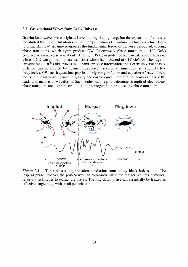
Figure 2.3. Three phases of gravitational radiation from binary black hole source. Theinspiral phase involves the post-Newtonian expansion while the merger requires numericalrelativity techniques to extract the waves. The ring-down phase can essentially be treated aseffective single body with small perturbations.
13

3 Gravitational Radiation
Gravitational radiation is fundamentally ripples in space-time, which travels with speed oflight and cause distance between free falling objects to vary. The distance between floatingobjects is stretched and squeezed by a passing wave. It can be lensed, red-shifted andscattered (significantly by massive dense objects like black holes) like the electromagneticwaves. However absorption and dispersion of GW by matter is negligible which is the reasonwave can travel without hindrance through galactic nuclei and massive stars. The essentialnon-linearity adds complexity to the problem.
The basic assumption before treating any cosmological problem, that universe is isotropic andhomogenous on large scale is our guiding principle. This endorses that the average curvatureof universe is intrinsically the same. We have clues about curvature of universe globally. Wemay reason that the universe may have zero (flat), positive or negative curvature. Howeverthe problem of determining the curvature locally is extremely difficult due to non-linearity ofgravity. The information provided by the Riemann curvature tensor in this regard is extensiveas suggested by general relativity. We can define such a tensor conveying information aboutcurvature of universe globally. A gravitational wave also contributes to the curvature of theuniverse. However, scales of contribution for both curvatures may vary largely. Tomathematically elaborate the concept of gravitational waves we need to consider how thecurvature of the universe can be conceived and how it adds to the Riemann tensor which istreated by short wave approximation [2,7]. 3.1 Short Wave Approximation
A major problem concerning gravity is its non-linearity. It is not possible to precisely separatethe contribution of GW from the curvature of space-time. The length scales on which it varies(GW) is much shorter compare to all other important curvatures in astrophysical situations.This significant difference make possible to split the Riemann tensor into two, one isbackground (R
B ) part and other is GW part (R GW ). The split is not analytically accurate
but it's a very worthy approximation. The R B can be regarded as the global large scale
average curvature of universe over several wavelengths. R GW is the rapidly changing part
of the Riemann tensor describing small scale curvature locally. The following expressionsestimate their respective scales
RB ~ 1
R2(3.1.1)
RGW ≡R−R
B ~ hƛGW
2(3.1.2)
where R is the Ricci scalar and ƛGW is the wavelength of GW divided by 2. We haveconsidered R
B inversely proportional to R2 assuming a closed universe, like the curvatureof closed sphere is defined as inverse square of its radius. We can have an approximation ofhow the magnitude of two parts of Riemann tensor differ, following calculation for the GWwavelength probed by LIGO (h~10−22) can be done.
14

1R2~
11056 cm2
(3.1.3)
R GW ~ h
ƛGW2 ~ 10−22
108 cm2~1
10−38 cm2 ≫1
1056 cm2
(3.1.4)
where R is approximated by Hubble radius of universe. This powerful method of definingGW part of Riemann tensor was introduced by Wheeler and Power (1957) and is known astwo length expansion or short wave approximation. The pertinent result is that GW trulybehaves in the same way as electromagnetic waves in vacuum.
Figure 3.1. Shows a closed universe scenario where metaphorically the closed world is likean orange and its surface ripples are like scale of GW wavelength.
3.2 Equation of Geodesic Deviation
To illustrate how the incoming wave influences the free-falling particles we need to considerhow the geodesics of two particles deviate. We will derive the fundamental equation forgeodesic deviation in terms of the Riemann tensor. We can assume two free-falling pointparticles A and B as shown in the Figure 3.2. with their respective trajectories xandx. By geodesic equation for a particle we have their corresponding equations.
Figure 3.2. Two particles A and B moving through space-time
d2 x
d2 d x
dd x
d(3.2.1)
15

d2xd 2
xd x
dd x
d(3.2.2)
Taking the difference of these two equations mentioned above and ignoring second and higherorder terms in we can simply derived the equation for geodesic deviation.
Du Du=R
UU (3.2.3)
where U=d /d is the velocity of particle and Du is the associated covariant derivative.
3.3 Mathematical Description of Gravitational Wave
Lets consider two test particles A and B in nearly flat Minkowski space-time. Particle A is inrest in the local Lorentz frame of our observer. As the gravitational waves passes, the particleB appears to be moving as seen by observer shown in the Figure 3.3.
Figure 3.3. In local Lorentz frame of A, particle B seems to moving when GW is passingwhere metric tensor g is approximated by the considering closed Friedmann Walkeruniverse scenario and assuming ∣R∣~1 /R2.
Let i be the general coordinate distance, then the variation in distance when GW are passingby is
i=0i i (3.3.1)
where 0i is the initial distance before the wave. By the condition of geodesic deviation
(3.2.3) we have
∂2
∂ t 2 i=−R 0j0
i j (3.3.2)
As there was no relative motion between particles A and B before, (3.3.2) by aid of (3.3.1)reduces to
16

∂2
∂ t 2 i=−R 0j0
i j (3.3.3)
Remember that in local Lorentz frame all the components of the Riemann tensor aredetermined by Ri0j0. By defining the field metric
−R 0j0i =1
2¨hijTT (3.3.4)
we can simplify the expression
∂2
∂ t 2 i=1
2 ¨hij
TT j 0 (3.3.5)
or
i=12hij
TT j 0 (3.3.6)
Now to visualize how the passing GW effect free floating particles, we will consider thefollowing scenario. When the wave is propagating only in the z-direction, the effect on x-yplane circle can be explained by (3.3.6). We have a set of four equations for our current circle.The expressions can be categorized as two modes of vibration (plus and cross modes)depending on the value of field. Figure 3.4 illustrates the effect of this passing wave. For theplus mode of vibration the equations are
x= 12hplus
TT x 0 (3.3.7)
y=−12hplus
TT y 0 (3.3.8)
Similarly, for the cross mode we have
x=12hcross
TT y 0 (3.3.9)
y=12hcross
TT x 0 (3.3.10)
17

Figure 3.4. Considering points on a circle in x-y plane. As GW passes in z-direction howdistance between points varies is shown for the both modes of vibration. It is apparent thatfield reinstate its initial configuration after cycle of wave.
3.4 Linearised Einstein's Equations
Einstein's equations by equivalence principle are given by
G≡R−12
R=8T (3.4.1)
where T is the energy momentum tensor, R the Ricci scalar and R the Ricci tensor. TheEinstein's equations can be thought as 10 coupled second order partial differential equationsfor ten metric tensor components. Again the non-linearity makes it demanding to find anexact solution of Einstein's equations. The best way to understand wave nature of GW is byfinding a solution of Einstein's equations (3.4.1) in a linearised regime [28]. We will assume aregion far away from any source which is nearly flat regime. The metric can then beexpressed as sum of Minkowski flat metric plus small perturbations.
g=h (3.4.2)
where is Minkowski space-time with metric signature =−1,1,1,1 and perturbationsare small ∣h∣≪1 . Partial derivatives of the metric can readily calculated as
g ,=,h ,=h , (3.4.3)
We know the general expression of Christoffel symbols in terms of metric tensor
=1
2gg , g,−g , (3.4.4)
We can linearised expression this expression with the aid of equations (3.4.3) and (3.4.2)
=1
2h ,h ,−h ,
= 12h ,
h , −h ,
(3.4.5)
Another expression we need is of the Riemann curvature tensor in terms of Christoffelsymbols
R= , − ,
−
(3.4.6)
by use of the (3.4.5) and by neglecting the second and higher order term which is valid for thelinearised regime, (3.4.6) reduces to
18

R= , − ,
= 12h ,
h , −h,
h, (3.4.7)
Moreover, the Ricci scalar can be approximated as
R≡gR≈R (3.4.8)
By use of (3.4.8), (3.4.7) and substituting it in (3.4.1) we have
h , h ,
−h ,h,−h
−h,=16T (3.4.9)
For the purpose of simplification, we will define new trace inverse metric tensor
h≡h−12h (3.4.10)
solving again (3.4.9) for this new metric, we acquire our equation
h
h− h,
− h,=16T (3.4.11)
Now using the Lorenz gauge condition h,=0 we have finally our desired result.
h=−16T (3.4.12)
which has the familiar Green's function as a solution
h=−4∫Tx ', t−∣x−x '∣∣x−x '∣
dV ' (3.4.13)
The simplest solution one can have for (3.4.13) is plane wave solution of the form
h=ℜAeika xa
(3.4.14)
where A is the polarization tensor and k= ,k, with the gauge conditions
kk=0 (3.4.15)
kA=0 (3.4.16)
Using the Lorenz gauge condition we can determine the only radiative components of thefield metric ( h
TT ), so we reduce to transverse traceless gauge. If we assume the wave travelsin the z -direction and by imposing the gauge conditions (3.4.15) and (3.4.16) we have
19

A0 z=Ax z=Ay z=Az z=0 (3.4.17)
for the linear regime equation (3.4.16) can be rewritten as
A=0 (3.4.18)
which implies the condition
Axx=−Ayy (3.4.19)
By conditions (3.4.17) and (3.4.19) we finally have our polarization tensor.
A=0 0 0 00 Axx Axy 00 Axy −Axx 00 0 0 0
(3.4.20)
The polarization tensor (3.4.20) indicates that we reduce to just two degrees of freedom intransverse traceless gauge which are intrinsically two (plus and cross) modes of GW.
Aplus=0 0 0 00 1 0 00 0 −1 00 0 0 0
(3.4.21)
Across=0 0 0 00 0 1 00 1 0 00 0 0 0
(3.4.22)
Figure 3.5. Fields lines for the plus and cross modes of GW can be represented like theelectromagnetic field lines.
Table 3.1. Comparison of transformation of electromagnetic and gravitational field byrotation of angle θ as shown in Figure 3.5. The helicity for electromagnetic waves is 1 and forGW is 2. Transformation of a field by a rotation of angle θ is '=ei h where h is thehelicity of the field .
Electromagnetic waves Gravitational waves
Exnew=Ex cosEy sin
Eynew=Ey cos−Ex sin
hplusnew=hplus cos 2−hcross sin 2
hcrossnew =hcross cos2hplus sin 2
20

Figure 3.6. Rotation of an electric field by an angle θ
3.5 Multipole Moments Decomposition
Multipole expansions are useful express to any field potential around any source in seriesexpansion which often can be truncated to some term. The same is true for the gravitationalfield of mass source as well as for electromagnetic field around a point charge. For detaileddiscussion on this topic, see [5,12]. First we will describe how the multipole expansion ofMaxwell's equations can be done which eventually guides us how to expand a classicalgravitational field. Maxwell's equations can be written in covariant form as
∂F=J (3.5.1)
F=∂A−∂A (3.5.2)
where A=/c2,−A and J= ,J , by substituting (3.5.2) in (3.5.1)
∂∂A−∂∂
A=J (3.5.3)
Again exploiting the gauge freedom we have, Lorenz gauge simplifies the expression (3.5.3)
∂∂A=−J (3.5.4)
(3.5.4) has the famous Green's function as a general solution
Ax , t =−∫ Jx ' , t−∣x−x '∣/c
∣x−x '∣dV '
(3.5.5)
Now considering a region far away from the source such that ∣x∣≫R, where R is the size ofthe source. The power series expansion of factor ∣x−x '∣−1
1∣x−x '∣
= 1x−x '2
= 1
x2−2xx ' x '2= 1∣x∣
2 x '.n 1∣x∣2...
(3.5.6)
21

where n=x /∣x∣. Now consider the retarded time factor as nearly constant we can expand thedifference as
t−t0=∣x∣−∣x−x '∣/c=−n .x ' /cO∣x∣−1 (3.5.7)
hence by (3.5.7) the J term in (3.5.5) can be Taylor expanded in terms of time derivatives as
J t0−∂ t J t0n⋅x ' /c∂tt J
t0n⋅x '2/2c2... (3.5.8)
only considering the dominant mode ∣x∣−1 term in (3.5.6), (3.5.5) can be written in terms oftime derivative of current source
A=−∣x∣−1
4 ∫J t 0−∂t J t0n⋅x ' /c∂tt J t0n⋅x '2/2c2...dV '
(3.5.9)
Now in (3.5.9) ∫ J t0dV the first term is the total charge which is constant.
∫∂ t J t0 n.x ' /c dV=n.∂ t∫ Jx ' dV ' second term is derivative of dipole moment which is
dominant in electromagnetic radiation. Now we will discuss how this procedure can beextended to gravitational field. Gravitational forces in Newtonian regime satisfies Poissonequation
∇ 2=4G (3.5.10)
Now, a 4D variant of above equation has Green's function as general solution
x , t =−G∫x ', t−∣x−x '∣/c∣x−x '∣
dV ' (3.5.11)
Similar to (3.5.9) power series expansion, (3.5.11) can be written in form of series.M=∫dV ' first term in the series is total mass of the system. P=∫∂ tx 'i dV ' second
term is just the total momentum of the system which is also conserved. Iij=∫∂ tx 'i dV 'third term is the quadrupole moment which is the first term appears in radiation field. Hencethe field potential can be approximated by
≈−GM∣x∣
G n⋅Pc∣x∣
−G Iij n i n j
2 c2∣x∣
(3.5.12)
We can only have the only radiative component of (3.5.12) as dimensionless gravitationalfield
h≈−G Iij ni n j
2 c4∣x∣
(3.5.13)
22

But to characterize the component of gravitational field which propagates, it has to betransverse and traceless
h ij≈−G Iij n i n j
2 c4∣x∣
(3.5.14)
where Iij=Iij−1 /3ij Ikk trace removed. To estimate how much energy is carried away bythese waves we associate the flux ( F ) with them
F= −14G
n⋅grad (3.5.15)
In local wave zone, where the n⋅grad ≈−, the expressions for flux of waves and itsrespective luminosity are
F= 14G
2= c3
4Gh2
(3.5.16)
L=4 ∣x∣2 F ~ G4 c2
I2 (3.5.17)
The expression (3.5.17) for luminosity is a good approximate for the full general relativityresult. The rate of energy carried by the waves can be given by expression
dEdt
=−∫TGW0r dA (3.5.18)
where TGW0r is the energy momentum tensor for GW at radial distance r. So in the local wave
zone this expression takes form of this famous result
dEdt
=− 132∫⟨ hij
TT hijTT ⟩dA (3.5.19)
or
dEdt
=− G5 c2∫ ⟨ Iij Iij ⟩dA
(3.5.20)
3.6 Expansion in Source Region for Slow Motion Sources
The method of multipole expansion can be expanded to the slow motion sources andconsidering field points far away from the source. By slow motion sources we mean whenvelocities are negligibly small compared to the speed of light. Such conditions are met bypulsars, where speeds are non-relativistic. Instead of multipole expansion of factor ∣x−x '∣−1
we will approximate this as r. Thus, (3.5.11) can now be Taylor expanded in terms of r. Theexpansion series for the gravitational potential can be given in terms of time derivatives ofsource mass density
23

=−G∫ 1r ∑n=0
n=∞
− rc
n 1n!
dn
dtn x ', t dV' (3.6.1)
We will expand the series and look for the possible dynamical terms in the expansion. Thefirst term is just the Newtonian potential term.
N=−G∫ 1rdV ' (3.6.2)
The second term does not contribute either.
Gc ∫dV '=G
cddt∫dV'=0 (3.6.3)
The third term is the first post-Newtonian term.
PN1=−G
2 c2∫ r dV ' (3.6.4)
The fourth is a term with a factor of r2 which suggests it is independent of x so it does notcontribute either.
G3c3∫ r 2 dV '= G
3 c3∫∣x∣2−2x⋅y∣y∣2 dV ' (3.6.5)
Figure 3.7. A far away field point from slow moving source
The fifth term is the second post-Newtonian term.
PN2=−G
c4 4!d4
dt4∫ r3dV ' (3.6.6)
At sixth term of the series radiation reaction is seen. This term is referred as 2.5 post-Newtonian term. However, gravitational field h has to be decomposed in terms of both sourcemass and mass current distributions which is being valid through weak field near zone andlocal wave zone (see figure 3.8 for description various wave zones). Let
M0, M1, M3. .. S0,S1,S3. .. are the mass and current moments of source respectively thenschematically in local wave zone, h can be decomposed as
h~M0
r
M1
r
M2
r...
S1
r
S2
r...
(3.6.7)
where h falls as 1/r
24

M0 mass cannot oscillate M1 momentum cannot oscillate M2 first term is mass quadrupole moment S1 angular momentum cannot oscillate S2 current quadrupole term is dominant for neutrons stars
Similarly, for the weak field near zone decomposition can given by
h~M0
r
M1
r2 M2
r3 ...S1
r
S2
r2 ... (3.6.8)
Table 3.2. Comparison of various post-Newtonian terms mentioned with their effects.Term EffectsNewtonian KeplerPN
vc
2 Perihelion shift
P1.5N v
c3 Spin-Orbit coupling (Frame drag)
P2N v
c
4 Spin-Spin coupling
P2.5N v
c5 Radiation reaction
Any gravitational field around a mass source can be categorized into wave generation andwave propagation zones. Thus, dividing the region into zones so that we can be safely applydifferent set of mathematical tools for both. An inner radius rI encompassing the wavegeneration zone (weak field near zone and strong field region) and on the other hand outerradius ro defining the inner boundary of wave propagation zone (distant wave zone). However,these two zones overlap in local wave zone defined by radius rI≤r≤r0. The inner radius rI isfar away from the source (rI≫ƛ) such that gravity of the source is weak. The outer radius ro
is far away from inner one (ro−r I≫ƛ), but not that far away that gravitational redshift andbackground curvature significantly affect the propagation. Weak field near zone is defined byradius (2M≪r≪ƛ) and strong field zone by r≤M. The expansion we have dealt with isvalid in the local wave zone and weak field near zone of radiation. The gravity field in strongfield zone is so strong in magnitude and non-linear in character that such expansions are notanymore accurate. Numerical treatment of Einstein's equations is the only method which cansafely be exploited in strong wave zone. The treatment of numerical relativity for strong zonewill be dealt in Chapter 5. The various wave zones around source mass are depicted in figure3.8.
25

Figure 3.8. Depicting various wave zones around mass source and techniques applied foranalysis, see [28,2].
4 Post-Newtonian Approximation
4.1 Post-Newtonian Approximation
The main objective of this section to explore how we can manipulate the post-Newtoniantechnique to determine the various observables associated with a gravitational wave. The two-body problem we are considering here is black hole binaries, which are inspiralling aroundthe centre of mass. The energy of the system is lost by the outgoing radiation. Thegravitational reaction forces the two black holes to come closer and closer into a downwardinspiral and eventually merge to form a single black hole resulting in a burst of radiation. InFigure 2.3 various stages of binary black hole coalescence are shown. The purpose of thewhole effort is extract waves and compare them with the signals received by the ground baseobservatories which will assist in accurate understanding the binary black hole problem. Thischapter is an adaptation of [4].
The most successful theory of gravitation, general relativity has failed to provide an exactsolution to two body problem. Numerical techniques are the only hope for an approximateunderstanding of binary dynamics. One outstanding technique is the post-Newtonian (PN)approximation in which flux (F) of the gravitational waves is obtained by a series expansionin parameter v /c=GM / r c2 where v is the source velocity and r(t) Schwarzschild radialdistance between black holes. The PN approximations are highly successful in obtaining thedecay of binary pulsars with the emission of GW [4,6,24]. However binary pulsars don't testthe PN theory to highest order as the relativistic velocities of pulsars are small (v /c~3×10−3
). The approximation is valid for the inspiral regime where the parameter is small. Currentlythese expressions are known up to 3.5 PN order (where vn corresponds to term of n/2 PNorder). The expressions of wave flux F and non-relativistic energy E can be given in terms ofseries in v
26

E=−12v2∑
k=0
∞
Ek v2k (4.1.1)
F= 3252 v10∑
k=0
∞
Fk vk (4.1.2)
where =m1 m2/m1m22 symmetric mass ratio for binary with masses m1 and m2. Ek and
Fk (expansion coefficients) are only functions of η. The method assumes adiabaticapproximation which insures that the fractional change of orbital velocity over an orbitalperiod is negligibly small ( /≪1 ) and luminosity of radiation is proportional to rate ofchange of orbital frequency. For the circular orbits the energy balance equation is
F=−M dEdt (4.1.3)
One would use the following coupled differential equations for the evolution of the orbitalphase
ddt
− v3
M=0
(4.1.4)
dvdt
FvM E 'v
=0 (4.1.5)
where we have used the fact that (orbital phase) which is the half the gravitational wavephase in restricted waveform at dominant order and v3=M f where f is frequency ofGW. Solutions to these ordinary differential equations are
t v=t0M∫v
v0 E 'vFv
dv (4.1.6)
v=0M∫v
v0 E 'vFv
v3 dv (4.1.7)
where t0, ɸ0 are integration constants, v0 is a reference velocity and E 'v=dE v/dv. Allthat is left is to estimate the expressions (4.1.6) and (4.1.7) with various orders of F(v) andE'(v) in terms of series and solve the differential equations (4.1.4) and (4.1.5) with numericaltechniques. Currently, the expressions for the E(v) and F(v) are known up to 3 PN and 3.5 PNorders respectively.
E3 v=−12v2[1− 3
4 1
12v2− 27
8−19
8 1
242v4E3 v6]
(4.1.8)
F3.5 v=3252 v10 [1− 1247
336 35
12 v2−4 v3F4 v4F5 v5F6 v6F7 v6]
(4.1.9)
27

where expansion coefficients are
E3=− 67564
− 34445576
−2052
96 15596
2 355186
3F5=− 8191
672583
24
F7=− 16285504
− 2147571728
−1933853024
2F6=
664373951969854400 16
3 2−1712105 41
48 2−134543
7776 −944033024 2−775
324 3−856
105 log 16 v2
and =0.577216 ... is the Euler constant.
4.2 TaylorT2 The expression of E'(v)/F(v) in equations (4.1.6) and (4.1.7) has to be truncated up to validPN order. Evaluating the expressions by integrating them one would obtain the followingexpressions for 3.5 PN order.
3.5 v=0−132v5 [ 13715
1008 5512 −10 v315293365
1016064 271451008 3085
144 2 v4 +
38645672 −65
8 ln vvlso v51234861192645118776862720 −160
3 2−171221 v6 +
225548 2−15737765635
12192768 760556912 2−127825
5184 3−85621 log 16 v2v6
+
7709667520321128
37851512096 −74045
6048 2v7]
(4.2.1)
t3.5v=t0−5M256v8 [1743
25211
3v2−32
5 v33058673
5080325429
504617
722v4 +
7729252
−133
v5−10524698566912347107840
1283
26848105
31475531273048192
−45112
2v6
−152111728
2255651296
33424105
log 16 v2v6−15419335127008
−75703756
14809378
2 v7 ]
(4.2.2)Both expressions have transcendental functions which require lot of computation power forobtaining high resolution waveforms. For simulation purposes, t0 can be chosen to be time ofcoalescence for binaries. By reverting (4.2.2) the expression, v(t) can be found by determiningroots of polynomial of v for a given time interval.
28

Figure 4.1. The v t2 is extracted by reverting the expression (4.2.2) and finding the rootsfor given time interval, considering it as a polynomial in v t 2. Here time for coalescence is32s for M=1.4 binaries. The v t 2 represents a much accurate description of amplitude ofgravitational waveforms.
4.3 TaylorT3
As shown in section 4.2 by finding the explicit expression for v and t v one wouldrevert the expression (4.2.2) and can determined v t . The equations for orbital phaseand instantaneous frequency of GW for 3.5 PN then can obtained as
3.5t =0−15 [ 3715
8064 5596 2−3
4 3927549514450688 284875
258048 18552048 2438645
21504 −65256 ln lso 5
+83103245074935757682522275840
−5340
2−1265100898854161798144
22552048
2−10756
1545651835008
2 6
+−11796251769472
3−10756
log 26−189516689433520640
−97765258048
1417691290240
27]
(4.3.1)
f 3.5=2
8M[1743
268811
322−3
1031855099
1445068856975
258048371
204824−7729
21504−13
2565
720817631400877288412611379200
53200
2107280
25302017977416178144
−4512048
2 −309131835008
26 +
2359251769472
3107280
log26−188516689433520640
−97756258048
1417691290240
27]
(4.3.2)
where = t 0−t /5M −1/8 and f ≡2 '2−1=v3/M . Given value of t0 one can findorbital phase and frequency of gravitational waves. As t t 0 frequency (F t ) diverges.
29

Figure 4.2. The instantaneous phase ( t ) and frequency ( F t ) of gravitational wavefor M=1.4 binaries with t0=32sec are shown. The order of instantaneous phase wastruncated up to 4 term. It's evident that F t diverges at t t 0. 4.4 Extraction of Binary Inspiral Waveforms
The inspiral waveforms can be extracted by the expression
h t =Apcos 2t Ac sin 2 t (4.4.1)
where Ac, Ap and are the amplitude of cross-polarised and plus polarised GW. The expressionfor 3.5 t was truncated up to 4 term. The amplitude, A(t) is given by the response ofantenna to the gravitational wave as given by expression
A t =4 C MC
DLMc f GW t
23
(4.4.2)
where MC=3 /5m1m2, DL is the luminosity distance, C (0≤C≤1) is geometric factor thatdepends on the orientation angle between antenna and binary system. By (4.4.2) explicitexpressions for Ac and Ap can be determined as
Ac t =−2 C MC
DL2 cosi Mc f GW t
23
(4.4.3)
Ap t =−2 C MC
DL1cosi 2 Mc f GW t
23
(4.4.4)
where i is the inclination angle of binary with earth.
30

Figure: 4.3. Gravitational waveform for M=1.4 binaries with t0=32sec and i=0 isshown. The waveform were extracted by (4.4.1) considering C as unity. It's evident fromspectrogram that the frequency diverges as time of coalescence is reached.
Another more realistic way to extract waveform is by exploiting the expression
h t =v t2 cos 2 t (4.4.5)
which is a much more accurate description of GW amplitude in comparison to above method.The reason for being such a nice waveform is that amplitude varies dominantly proportionalto v t2. The results for such waveform are shown in Figure 4.4.
Figure 4.4. Gravitational waveform for M=1.4 binaries with t0=32sec is shown. Thewaveform were extracted by (4.4.5). The evident feature of waveform is its non-zero contentand smooth variation.
4.5 Extraction of Waveform by Stationary Phase Approximation
In restricted PN approximations only PN corrections to the phase are included and amplitudecorrections are neglected. The response of antenna to a gravitational radiation is given by
h t =A t cos t (4.5.1)
31

where A(t) is given by (4.4.2). The purpose of neglecting amplitude corrections simplifies theprocess of data analysis to a large extent. For our purposes, Fourier domain is a good choiceto work with, Fourier transform of (4.5.1) yields
h f =A t ∫−∞
∞
e2ift e−i tei tdt=A t ∫−∞
∞
ei2ft− tei2ft tdt (4.5.2)
expression (4.5.2) can be dealt with as stationary phase approximation. It's the far mostpopular way of extracting the waveforms, the approximation yields
h f = CDL
2 /3524
MC56 e
if i4
(4.5.3)
where
f =2f t00∑k=0
7
k f k−5/3 (4.5.4)
and the expansion coefficients for f in (4.5.4) are given by
k=3
128Mk−5/3 k
0=1, 1=0 , 2=3715756
559 , 3=−16 , 4=
15293365508032
27145504
308572
2,
5= 38645756
−6591ln 63 /2M f
7= 77096675254016
3785151512
−74045756
26=
115832312365314694215680
−6403
2−684821
−157377656353048192
225512
2 +
760551728
2−1278251296
3−684863
ln 64M f
The coefficients 5 and 6 are not constant as they have log f-dependence but we can treatthem as constant if we assume that log f-dependence is weak in the desired bandwidth. Forsimulations the expression for f was evaluated up to k=2.
However, computations as suggested by (4.5.3) produce some artifacts (spurious frequencies).These artifacts has to be removed by truncating frequencies greater then f0 . To produce therequired waveform in time domain inverse Fourier transform has to be performed which againgenerate some false frequencies in waveform. Bandpass filtering has to be performed to throwaway some of lowest and highest false frequencies. The results are shown in figure 4.5.
32

Figure 4.5. The waveform was extracted by the stationary phase approximationprocedure described in this section. The waveform are obtained for M =1.4 binarieswith t0 = 32 s.
Figure 4.7 (a). Amplitude of cross and plus polarised gravitational wave at i=0
Figure 4.7 (b). Amplitude of cross and plus polarised gravitational wave at i=90
33

5 Numerical Relativity
In general relativity the two-body problem is of special interest. The binary black holeproblem has become exciting and challenging in astrophysics. On the successful operation ofdetectors all around the world, interest is growing on receiving signals from supernovaebursts, star collapse and binary black holes coalescence. But one major issue with GW is itscomplexity to extract waveform and weakness of received signal. Numerical relativity plays avital role to extract waveforms from background noise by matching with already existingwaveforms banks. The interest is growing due to the exponential increase in computationalpower of clusters over the past decades. The binary black hole in vacuum are the primarysources of gravitational radiation. We already have discussed briefly various phases of thebinaries resulting in signature waveforms. Post-Newtonian approximation is one the effort tosolve the issue. But this method has its own limitations in strong gravitational interactions andat relativistic speeds. The sole purpose of numerical relativity is to solve Einstein's equationsby numerical techniques for various astrophysical scenarios. The final stages of black holecoalescence involve strong gravitational interactions where only numerical relativity methodsare valid. Post-Newtonian approximations are not useful at such extreme curvatures andrelativistic speeds.
In 1964, the first attempts to solve Einstein's equations by numerical techniques werereported. But at that time the computational resources needed to solve the problem wereinadequate. Now we have the computational power and memory to solve the Einstein'sequations computationally. Advance algorithms for solving such complex problems has beendeveloped over decades. Our interest in numerical relativity is to extract waveforms frombinary black hole evolution and form a template bank which can be utilize to matched withthe received signals. Due the technological advancement in supercomputers, this field isbecoming increasing mature and lot of previous problems are reconsidered. Collision ofaxisymmetric black holes, binary black hole inspiral, and coalescence of black hole withinitial spin and momentum are being studied. The evolution times are being enough to extract
34

the gravitational waveform. However the simulations of binary black holes space-time turnout to be much more complicated due to the computational challenges they pose.
Einstein's equations can be considered as ten coupled non-linear partial differential equations.The equations can have many equivalent forms. In harmonic form, the metric tensor formswave equations which are mathematically known for their stability properties. The metrictensor cannot be decomposed into background and perturbations for strong gravity scenarios.Therefore, numerical solution to Einstein's equations is the way forward. There are only sixcomponents to be solved for metric the rest of four components are just gauge freedom. The3+1 split of metric tensor is the basis for the ADM formalism. The BSSN formalism is theconformal modification to this formalism. BSSN has developed interest in the two-bodyproblem because of the stability of evolution on supercomputers. Dealing with space-timesingularities is another issue which is to be resolved by method of excision. Excision isaccomplished by excluding space points which are causally disconnected but this methodcomes with a price. Keeping track of apparent horizons at each time step to perform excisionis computationally expensive. The excision can be avoided by using puncture initial data forevolution. We will systematically discuss some of the formalism, initial data and findings inthis chapter. This chapter is based on systemic study of [1,8,9,10,11,13,14,15,16,17,18,19,26].
5.1 Arnowitt-Deser-Misner (ADM) Formulation
The 3+1 split of Einstein's equations is the most widely used formulation in numericalrelativity. Space-time is foliated by considering spacelike hypersurfaces which evolve withcoordinate time. So the four-dimensional space-time is split into three-dimensional hyper-surfaces plus time. The idea was first suggested by Arnowitt, Deser and Misner when theywere trying to quantize gravity. The technique we will discuss is Cauchy approach which seesspace-time as three dimensional space at particular instant of time. To grasp the concept wewill first consider 3+1 split of Maxwell's equations. The famous Maxwell's equations can bewritten in terms of vector potential A a set of three equations
∇⋅E=4 (5.1.1)
∂ A∂ t
E∇=0 (5.1.2)
−∂ E∂ t ∇×∇×A=4J
(5.1.3)
The above set of equations can be categorized into two. The ones which are constrained andthe ones which are evolution equations. (5.1.1) is a constraint equation which cannot beviolated at any instant of time as the evolution continues. (5.1.2) and (5.1.3) are the evolutionequations which determines the evolution of fields as time progress. However if the evolutionis performed numerically then it cannot be guaranteed that the constraint equations will not beviolated.
Now we will continue to 3+1 split of Einstein's equations. The four-dimensional space-time isfoliated by three-dimensional hyper-surfaces Σ which are labelled by t. n
is a normal vector
35

on hyper-surface which points in increasing value of time. We can define a projection tensorP which projects any vector to spatial the hyper-surface Σ. Following are the straight
forward properties of such a tensor
P≡g−nn (5.1.4)
P=P (5.1.5)
Pn=0 (5.1.6)
The P must be symmetric and should be purely spatial as indicated by (5.1.6). Nowprojecting the metric tensor to the hyper-surface we will have our spatial metric.
ij=Pi Pj
g (5.1.7)
The projections of time coordinate can be split into spatial direction and part orthogonal to it.
i=Pi t (5.1.8)
=n t (5.1.9)
Figure 5.1. Shows the two hyper-surfaces separated by coordinate time dt. The normal lineshow the direction of future pointing normal vector n. The coordinate line shows the samecoordinate on the two hyper-surfaces.
Therefore by (5.1.8) and (5.1.9) we have
t= n (5.1.10)
36

where α is lapse function which measure the proper time and is shift vector measuringvelocity of spatial coordinate labels. Now in terms of spatial metric, lapse function and shiftvector whole metric can be written in the form
ds2=−dt2ijdxii dtdx j j dt (5.1.11)
Another important quantity which needed to be defined for ADM formulation is extrinsiccurvature. Defined as projecting the covariant derivative of normal vector
Kij=Pi Pj
D n (5.1.12)
Another useful definition for extrinsic curvature is the Lie derivative with normal vector ofspatial metric
Kij=−12
Ln ij (5.1.13)
By help of above defined quantities we are now in a position to split the Einstein's equationsto formulate ADM equations
R 3K2−Kij Kij=16G (5.1.14)
D jKij−ijK =8G ji (5.1.15)
ddt
ij=−2Kij (5.1.16)
ddt−LKij=−Di DjRij
3K Kij2 Kil K jl8[Sij−
12S−] (5.1.17)
where L is Lie derivative with respect to i , R3 is the curvature tensor formed by 3Dspatial metric, Di is the covariant derivative, is energy density, ji is the momentumdensity, Sij stress energy tensor of matter and K is the trace of Kij. Again (5.1.14) and(5.1.15) are hamiltonian and momentum constraint equations. Whereas (5.1.16) and (5.1.17)are evolution equations for spatial metric and extrinsic curvature respectively. It's alwaysguaranteed by Bianchi identities that a initial solution to constrained equations will always bea solution to evolution equations at later times.
5.2 Baumgarte-Shapiro-Shibata-Nakamura (BSSN) Formulation
The ADM was considered as standard formulation for numerical relativity simulations untilrecently. As this formulation has some serious issues during the simulation. Evolution withADM formulation proved to be numerically unstable. Simulation with shorter evolution timewere reported. As the system approaches singularity in shorter time, numerical code crashes.BSSN reformulates the evolutions equations (5.1.16) and (5.1.17). This formulation has added
37

advantage of stability and longer simulation times. The basic idea behind this formulation isto split the conformal and traceless part of the ADM evolution equation. This is achieved byintroducing new spatial metric ij
ij=e−4ij (5.2.1)
to fix the determinant of metric to unity we have defined the following constrain
e−4=1/3 (5.2.2)
Instead of using extrinsic curvature we will consider its traceless part Aij which is defined as
Aij=Kij−13ij K (5.2.3)
Similar to conformal decomposition of spatial metric ij, Aij can be decomposed as
Aij=e−4 Aij (5.2.4)
The evolution equation (5.1.17) can be used to find trivial expression for conformal spatialmetric ij and its conformal factor as
ddt ij=−2 Aij (5.2.5)
ddt
=−16 K (5.2.6)
To find evolution equation for K, expression (5.1.17) can be used, with the aid of hamiltonianconstraint (5.1.14) the Ricci scalar is eliminated.
ddt K=−ij Di Dj[ Aij
Aij13 K2 1
2 S] (5.2.7)
For the evolution equation of trace-free part of extrinsic curvature some manipulation of(5.1.17) results in
ddt
Aij=e−4 [−Di D jRij−Sij]TFK Aij−2 Ail A j
l (5.2.8)
Due to the conformal decomposition of the spatial metric the Ricci tensor can also bedecomposed into conformal part and conformal factor as
Rij= RijRij (5.2.9)
The conformal factor Rij can be readily calculated by covariant derivatives of as
38

Rij=−2 Di D j−2 ij
Dl Dl4 Di Dj−4 ijDl Dl (5.2.10)
The conformal part Rij can be computed by the standard conformal spatial metric ij. Tosimplify matters, we need to define a new variable, conformal connection function as
i≡ jk jki =− , j
ij (5.2.11)
Now in terms of conformal connection i , Ricci tensor can be written
Rij=−12 lm ij, lm ki∂ j
k k ijk lm 2 l ( ik j )km i m
k klj (5.2.12)
Conformal connection function i must be promoted to independent variable as we want theexpression (5.2.12) of Ricci tensor to maintain its elliptic behaviour. However this comes witha price of computing three new evolution equations in the formulation. Assuming i asindependent variable the equation for its evolution can be given by
∂∂ t
i=− ∂∂ x j 2 Aij−2 m( j, m
i ) 23
ij, ll l , l
ij (5.2.13)
Still the above expression has stability issues when numerical simulations are done. Thesituation can be improved by removing the divergence of Aij with the help of momentumconstraint (5.1.16).
∂∂ t
i=−2 Aij, j2 jki Akj−2
3 ij K , j−ijS j6 Aij, j− ∂∂ x j
l , lij−2 m ( j, m
i ) 23 ij,l
l (5.2.14)
With this the evolution structure of BSSN is complete. The evolutions equations for , K , Aij , and i represents complete set of equations. The new formulation is much more
stable as the equations are well posed and have strong hyperbolicity.
5.3 Boundary Conditions
The computational domain of numerical relativity does not cover the whole space-time tospatial infinity due to lack of computational resources. Moreover, the domain covered by suchsimulation is pretty small such that boundary lies right where the space-time is dynamic.Therefore suitable boundary condition must be provided so to minimize the reflection andoutgoing waves leave the boundary smoothly. Such boundary must be set so that there are notartificial reflection and boundary conditions cause no instability. But this issue is not assimple as it seems due to several reasons. All dynamical variables do not behave as waves atsuch distances which are set by computational domain for simulations. Secondly, there are no
39

local boundary conditions which are provided for the incoming wave to leave the grid cleanly.We will now briefly discuss the boundary conditions (that can be set in Cactus (see section 5.6for details)) for binary black hole space-times.
Static Boundary Condition: By static we mean that at boundary no dynamical variable isupdated and they retain their initial values throughout the evolution. This condition is does theworse in our case and introduces lot of artificial reflection of gravitational waves. Howeverthe condition may suit such scenarios where static condition are required at boundary to avoidtruncation errors.
Flat Boundary Condition: Flat boundary condition allows some dynamics at the boundary ascompare to static condition but still introduces significant amount of reflections. When flatboundary is set the boundary value is just copied from a interior point where dynamicalvariable are calculated. Still this condition does no good for our purpose.
Radiative Boundary Condition: This boundary serves the purpose for a clean outlet ofwaves from the grid. It assumes that dynamical variable behaves like constant (f 0) plusoutgoing radial wave which decays as 1/r at the boundary of the grid.
f x , t =f 0u r−t r
(5.3.1)
where r=x2y2z2 , and f 0 is taken to one of diagonal elements of metric and rest arezero. The expression (5.3.1) clearly shows that we are assuming that outgoing waves behaveslike smooth wavefronts at the boundary. This boundary condition has found to be very usefulfor avoiding artificial reflections. However, there is more to it, to implement (5.3.1) itsdifferential form (5.3.2) is more useful in practice. As differential equations can beimplemented as difference in equations by numerical techniques.
x i
r∂ t f∂i f
xi
r 2 f −f 0=0 (5.3.2)
5.4 Gauge Conditions
The possible values of lapse and shift are one of the gauge choices which are needed to beprovided before the evolution. For gauge conditions we concentrate on the lapse function onlybecause shift vector is often chosen to be zero for our purpose. Determining the value forlapse function can be done in to three ways.
Prescribed Slicing: Specify the lapse initially for a given space-time by the known a priorconditions. The simplest example of such gauge is geodesic slicing. Gauge choice forgeodesic slicing is
≡1 and ≡0 (5.4.1)
40

The gauge choice simply suggests that it follows time-like geodesic with proper time ofEulerian observer. The geodesic slicing allows very short evolution times as coordinatesingularity is achieved at quite early stage. Like for Schwarzschild initial data singularity isachieved at M time. Shorter simulation times covers very small space-time domain thusextraction of gravitational wave is not possible which is not desirable.
Elliptic Slicing: This the most robust and accurate of form of slicing condition. Usually lapseis determined by solving elliptic differential equation on each time step by imposing somecondition on the spatial hyper-surfaces. However, solving elliptic equation on each time stepis a computationally expensive task.
Algebraic Slicing: The slicing calculates lapse and its time derivative on each hyper-surfaceas a function of spatial metric and extrinsic curvature. The slicing condition can becomputationally cheap. However it's difficult to analyse data analytically. The most commonused type of such gauge is hyperbolic K-driver condition. The lapse function is readilycalculated by
∂t−L=−2 FK (5.4.2)
The main advantages of such slicing condition is that it's cheap and lapse decays to zeros inregions of strong curvature. The typical choice for F is 2 / which is known as 1+logslicing. 1+log slicing the far most commonly used condition. It's cheaper for computers thenelliptic slicing condition and moreover foliates the action of singularity avoidance.
5.5 Initial Data for Black Hole
As we have developed suitable formulation for the evolution of black hole space-time andhave seen the constraint equations the natural question will be, which space-times satisfiessuch initial conditions and evolve with stability. To simplify the matters we are assuming thatextrinsic curvature Kij is set to zero. This condition simplifies matters a lot. Such assumptionmakes the momentum constraint trivial, however the hamiltonian constraint still needs tosolved. The requirement is that we want black hole to exist on initial hyperspace whicheventually evolve at time progress. For purpose of solving hamiltonian constraint ourassumption is that spatial metric ij is flat. This leads to simplification of hamiltonianconstraint as
D2=0 (5.5.1)
where the D covariant derivative associated conformal spatial metric ij. Solution to (5.5.1)leads to Schwarzschild and Misner initial data.
5.5.1 Schwarzschild Initial Data
Schwarzschild solved the Einstein's equations for a spherical symmetric vacuum space-time.The solution represents the exterior of a star or a black hole.
41

ds2=−1−2Mrs dts
2 1
1− 2Mrs
drs2r s
2 d2r s2sin 2 d2
(5.5.2)
The metric is a static solution to Einstein's equations as given in Schwarzschild coordinates (ts , rs , ,). To avoid the coordinate singularity, we can choose isotropic radial coordinatewhich is related to radial coordinate as
rs=1M2r
2
r (5.5.3)
The Schwarzschild metric in isotropic coordinates is given as
ds2=− 2r−M2rM
2
dt21M2r
4
dr2r2 d2 (5.5.3)
where d2=d2sin2d2. The spatial metric and conformal factor are set to followingvalues
gij=4ij (5.5.4)
=1M2r
(5.5.5)
For simulation purposes black hole resides at the origin of the grid. The isotropic lapsefunction has value 2r−M/ 2rM which can be set by using proper parameters in Cactus.However, isotropic lapse function retain its initial value throughout the evolution. Theevolution of Schwarzschild initial data can be treated as primary step to evolve more complexsystems, like coalescence of two black holes. Previously, this problem has been treatednumerically to gain experience for binary systems [18,19].
5.5.2 Misner Initial Data
In 1960, Misner proposed a way to represent space-time of two black holes. The solution canbe generalized to any number of black holes [17]. The metric represents two non-rotatingblack holes momentarily at rest and their throats are connected by two wormholes as show infigure 5.2. The two throats connected two asymptotic flat space-times. The throats can bethought as apparent horizons of black holes. The general metric for Miner data is given as
ds2=−dt24dx2dy2dz2 (5.5.6)
The conformal factor has the following solution to hamiltonian constraint for two throat data
= ∑n=−∞
∞ 1sinh 0 n
1 x2 y 2 zcoth 0 n2
(5.5.7)
42

However in practice the summation is cutoff to n =30, which is being tested for applicationsand works very well. The relations are given in cylindrical coordinates ( r , , z ).
Figure 5.2. The asymptotic flat regions are connected by two Einstein-Rosen bridges orwormholes representing the two black holes. Clearly, an isometry is there between upper andlower half of the two bridges.
0 determines the mass to throat separation ratio. If 0≃1.8, then black holes have the sameevent horizon. Similar solutions can be constructed for multiple black holes which has similarstructure of space-time as shown in Figure 5.2 but connected by multiple stationary throats.For Misner initial data, the relation for ADM mass is given by
M=4∑n=1
n=∞ 1sinh 0 n
(5.5.8)
5.6 Results and Discussion
The platform chosen for our simulation of binary black hole space-time is Cactus. Cactus isan open source framework developed for scientists and engineers which have the capacity torun on a wide range of architectures and operating systems. Cactus gives the power of parallelcomputing for challenging and exhaustive simulations with its modular structure of thorns.There are two components to Cactus the basic functional and interface is provided by fleshthe core module, while several other modules named as thorns have their respectivespecialized functionalities [13].
The emphasis of our simulation was on evolutions using the Schwarzschild and Misner initialdata sets. There were 100x100x100 grid points to cover the whole space-time. Each run wasdone with aid of both fixed mesh refinement (FMR) and adaptive mesh refinement (AMR)techniques. AMR capabilities were provided by Carpet which is designed to work seamlesslywith Cactus environment. The initial data were evolved by both BSSN and ADM formulationto test the reliability and crash times for code. ADM evolution is implemented in standardCactusEinstein thorns while BSSN functionality is provided by AEIThorns or CACTIE code.The Weyl scalars were extracted by PsiKadelia thorn measure the outgoing gravitationalwaves by the single static and dynamic binary black holes.
43

5.6.1 Schwarzschild Initial Data Evolution
The Schwarzschild black hole is a static solution to Einstein's equations. It represents theexterior of uncharged non-rotating black hole. However, this test run works as a benchmarkfor the code reliability and determining crash time. We have evolved initial data with ADMformalism based on FMR to about 17M with grid resolution of 0.2 and isotropic lapse. Suchevolution has no interesting dynamics in it but Weyl scalars extracted showed some form ofinstability which eventually crashed at about 17M. Similar evolution was performed with the1+log slicing and black hole mass of 1M. On contrary to isotropic lapse, such evolutionshowed some form of gauge waves. Perhaps, the reason for appearance of waves is that theresulting Schwarzschild isotropic metric was not in isotropic coordinates as it doesn't satisfy1+log slicing condition. But still the precise description of waves is not known.
(a)
44

(b)
Figure 5.3. Evolution of Schwarzschild initial data with grid resolution 0.2 and isotropiclapse where boundary was placed at 10M. (a) Real part of Weyl scalar 4 (outgoingtransverse wave) at 5M in x-z. (b) Real part of Weyl scalar 4 (outgoing transverse wave) at14M in x-z plane. Beyond that instability overcomes.
(b)
45

(c)
Figure 5.4. Evolution of Schwarzschild initial data with grid resolution 2 and 1+log lapsewhere boundary was at 100M. (a) The lapse contours at time 15M. (b) The lapse contours attime 30M. (c) Real part of Weyl scalar 4 (outgoing transverse wave) at 30M in x-z.
5.6.2 Misner Initial Data Evolution
This initial data is of most interest in our case. The data was evolved with both FMR andAMR grids. Similarly, both ADM and BSSN evolution sequences were executed with 1+loggauge conditions and 0=2.2. However, with BSSN the initial data was a lot more stable. Anobvious reflection appears at the boundary (at 10M quite near) when no boundary conditionwas set during BSSN evolution with grid resolution 0.2. The data was also evolved withboundary at 100M and grid resolution 2. During evolution, outgoing gravitational waves wereextracted by Weyl scalars.
(a)
46

(b)
(c)
47

(d)
(e)
48

Figure 5.5. Evolution of Misner initial data with grid resolution of 0.2 where boundary isplaced at 10M. (a) Lapse contour map at 1.5M with ADM evolution method using FMR.Lapse was initially set to unity. (b) Lapse at 7M for Misner initial data with ADM evolutionmethod using FMR technique. (c) Real part of Weyl scalar 4 (outgoing transverse wave) at7M in x-z plane using FMR, The reflection is not apparent at boundaries with ADMevolution. (d) Real part of Weyl scalar 4 (outgoing transverse wave) at 16M in x-z planeusing FMR, The wave reflection at the boundary is at its peak with BSSN formulation. Theapparent reflection is because no boundary condition was set throughout evolution andboundary has been place quite close. (e) Real part of Weyl scalar 4 (outgoing transversewave) at 20M in x-z plane, The wave reflection has been reduced due to radiative boundarycondition with BSSN evolution and AMR.
(a)
49
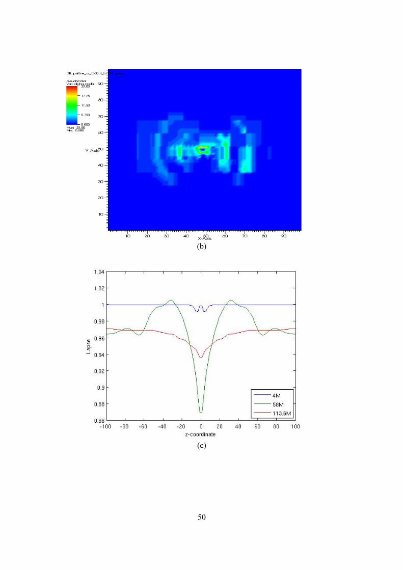
(b)
(c)
50

(d)
Figure 5.6. Evolution of Misner initial data with grid resolution of 2, where boundary isplaced at 100M. (a) Real part of Weyl scalar 4 (outgoing transverse wave) at 58M in x-zplane. (b) Real part of 4 at 113.6M. (c)Evolution of lapse. (d) Evolution of gxx.
6 Conclusion and Future Work
The overall objective of this thesis was to carry out a study on gravitational waves, lay thetheoretical foundation and test the findings by utilizing proper numerical tools available up todate. Due to the wide spectrum of this enriched area of study, it was impossible to evenexplore each and every subject in much detail. However, much have been done on extractionof gravitational waves during the inspiral and merger phase of the binaries. The pertinentconcepts are touched in much detail for the foundation of future work. The extraction ofwaves by post-Newtonian formalism and simulating binary black hole space-time along withthe extraction of Weyl scalars were explored with emphasis on computation.
The results obtained by aid of Cactus ware satisfactory. However, the emphasis of future workmust rely on latest numerical relativity scenarios. Evolution of puncture method, thinsandwich data and extraction of various modes of Zerilli waves (Zerilli wave equationdescribe perturbations of non-rotating black hole) by simulating binaries to much longer timesshould be considered in future developments. Much more realistic grid sizes can be chosenwhich eventually requires more memory and time resources on the cluster. Various topics inthis mature area are not even touched due to their complexity and shortage of time. Theexcision of black hole which is one of primary techniques of singularity avoidance is notmentioned in this thesis. Secondly, determination of black hole apparent horizons is also nottreated, as much of our work was focussed on extraction of gravitational waves. The field of
51

numerical relativity can be further explored by considering perturbed black holes, massiveblack holes inspiral and neutron stars merger.
References
1. Miguel Alcubierre, “Introduction to 3 + 1 Numerical Relativity”, Oxford University Press, 2008.
2. Kip S. Thorne, “Three hundred years of Gravitation: Gravitational Radiation”, Cambridge UniversityPress. 1987.
3. Robert M.Wald, “General Relativity”, Chicago University Press, 1984.
4. Alessandra Buonanno, Bala R. Iyer, Evan Ochsner, Yi Pan and B. S. Sathyaprakash, “Comparison ofpost-Newtonian templates for compact binary inspiral signals in gravitational-wave detectors”,Phys.Rev.D 80, 084043, (2009), arXiv:0907.0700v1
5. Kip S. Thorne, “Multipole Expansion of Gravitational Radiation”, Reviews of Modern Physics Vol. 52,No. 2, Part I, 1980.
6. Toshifumi Futamase and Yousuke Itoh, “The Post-Newtonian Approximation for Relativistic CompactBinaries”, Living Rev. Relativity, 10, (2007), 2.
7. Charles W. Misner, Kip S. Thorne and John A. Wheeler , “Gravitation”, New York: W.H. Freeman andCompany, 1973.
8. Jeffrey Winicour, “Characteristic Evolution and Matching”, Living Rev. Relativity, 12, (2009), 3.
9. Gregory B. Cook,”Initial Data for Numerical Relativity”, Living Rev. Relativity, 3, (2000), 5.
52

10. Beverly K. Berger, “Numerical Approaches to space-time Singularities”, Living Rev. Relativity, 5,(2002), 1.
11. Jonathan Thornburg, “Event and Apparent Horizon Finders for 3+1 Numerical Relativity”, Living Rev.Relativity, 10, (2007), 3.
12. Bernard F. Schutz, ”Gravitational Waves on the back of an envelope”, Am. J. Phys. 52, 412 (1984).
13. www.cactuscode.org
14. www.carpetcode.org
15. Michael Koppitz, “Numerical Studies of Black Hole Initial Data”, PhD thesis, University of Potsdam,2004.
16. Lars Nerger, “Investigations of 3D Binary Black Hole Systems”, PhD thesis, AEI, 2000.
17. Karen D. Camarda, “A Numerical Study of 3D Black Hole space-times”, PhD thesis, University ofIllinois at Urbana-Champaign, 1998.
18. Bernd Bruegmann, “Adaptive mesh and geodesically sliced Schwarzschild space-time in 3+1dimensions”, Phys.Rev.D54:7361-7372,1996, arXiv:gr-qc/9608050v1
19. Peter Anninos, Karen Camarda, Joan Masso, Edward Seidel, Wai-Mo Suen, and John Towns, “Threedimensional numerical relativity: The evolution of black holes”, Phys.Rev. D52 (1995) 2059, 1995.
20. Markus P. Rumpfkeil, “Elliptic Gauge Conditions in Numerical Relativity”, Phd Thesis, Max-PlanckInstitute for Gravitational Astrophysics, 2004.
21. Ulrich Sperhake, “Black hole binary evolutions with the LEAN code”, Journal of Physics: ConferenceSeries 66 (2007) 012049.
22. Michele Maggiore, “Gravitational Waves”, Oxford University Press, 2008.
23. www.chirplab.org
24. Luc Blanchet, “Post-Newtonian theory and the two-body problem”, arXiv:0907.3596v1
25. B.S. Sathyaprakash and Bernard F. Schtuz, “Physics, Astrophysics and Cosmology with GravitationalWaves”, Living Rev. Relativity, 12, (2009), 2
26. John Baker, Manuela Campanelli and Carlos O. Lousto, “The Lazarus project: A pragmatic approach tobinary black hole evolutions”, Physical Review D, Vol 65, 044001, 2002.
27. Scott A. Hughes, Szabolcs Marka, Peter L. Bender, Craig J. Hogan, “New physics and astronomy withthe new gravitational-wave observatories”, eConf C010630 (2001) P402, 2001.
28. Roger D. Blandford and Kip S. Thorne, ”Applications of Classical Physics”, 2008.
53

7 Appendix
A.1 Compiling and Running Cactus Framework
There are two important ingredients to setup framework for numerical relativity simulations.Primarily you will need to download Cactus [13] and compile it for your architecture anddepending on the compilers and additional softwares you require, this will take some effort.Then you will need to download Carpet [14], a adaptive mesh refinement functionality whichworks well with the Cactus framework. First you will need to download Cactus from thefollowing repository. I have tested this with OSX 1.6.2 with x-code 3.2. For this you need tohave CVS and git on you system. Just you need to issue following commands
cvs -d :pserver:[email protected]:/cactus login
54

You will be asked for password which is anon. After this you need to download Cactus fleshby command
cvs -d :pserver:[email protected]:/cactus checkout Cactus
Similarly, you can checkout the others arrangements. Before that you need to go toCactus/arrangements directory. The following arrangements are recommended and can bedownloaded by the following command.
cvs -d :pserver:[email protected]:/cactus checkout CactusEinsteinCactusWave CactusPUGH CactusPUGHIO CactusIO CactusExternal CactusConnectCactusBase CactusBench CactusTest
Second step is to download Carpet by the issuing following commands
cd Cactusgit clone -o carpet git://carpetcode.dyndns.org/carpet.gitcd arrangementsln -s ../carpet/Carpet* .
The last command is just to create a software link. If your system does not support suchcommand just create your own soft link and past it there. Before we continue to compiling,you need to have a C++/C and F77/F90 compiler. The best way you can get for your macsystem is by website http://hpc.sourceforge.net/. Please download GCC 4.4 and install it fromthe binaries. The next you need to have a visualization software which I recommend is VisIT.Go to website https://wci.llnl.gov/codes/visit/executables.html get the executable and copy theinstall script along with it. Place both in the same directory and issue the following command.Remember this command is for the mac systems as mentioned before. Otherwise you need tomake changes accordingly in the command.
sudo ./visit-install 1.12.1 darwin-i386 /visit
The third external software you need to have before we continue to compilation procedure isHDF5. Which you can get from http://www.hdfgroup.org/downloads. Get the current releaseof this software don't worry about the hdf5 software with the file streaming capabilities. Thethird repository you need to have is AEIThorns which you can have by
cvs -d :pserver:[email protected]:/numrelcvs loginCVS password: anoncvs -d :pserver:[email protected]:/numrelcvs checkout AEIThorns
Now for configuration of Cactus on you local OSX machine issue following commands onterminal.
Cd Cactusmake local-config HDF5=yes LDFLAGS=-lgfortran F90=gfortran F77=gfortranCC=gcc CXX=g++
This configures cactus with the config file name “local”. Make sure that cactus found theHDF directory and last test on compilers goes well. Now to compile this configuration write
make local
55

This will usually generate errors cause of incompatible thorns in your thorn list. So go toCactus/configs/local folder and edit Thornlist file (just copy the thorns given below toyou file and save it). The following thorns are recommended which are needed to be compilefor purpose.
AEIThorns/AEILocalInterp # AEILocalInterp ( ) [ ] { }AEIThorns/AEIUtil # AEIUtil ( ) [ ] { }AEIThorns/BAM_Elliptic # BAM_Elliptic AEIThorns/BAM_VecLap # BAM_VecLap AEIThorns/BSSN_MoL # adm_bssn AEIThorns/BoundaryExample AEIThorns/CalcK # CalcK (ADMBase,StaticConformal) [ ] AEIThorns/Constants # Constants ( ) [ ] { }AEIThorns/EHFinder # ehfinder AEIThorns/Exact # exact AEIThorns/FiniteDifferencing # FiniteDifferencing ( ) [ ] { }AEIThorns/Fortran # Fortran ( ) [ ] { }AEIThorns/HyperWave # HyperWave (grid) [ ] {MethodOfLines}AEIThorns/HyperWave0 # HyperWave0 (grid) [ ] { }AEIThorns/IDConstraintViolate # idconstraintviolate (admbase,grid) [ ]AEIThorns/IDFileADM # IDFileADM (ADMBase,StaticConformal,IO)AEIThorns/ManualTermination # ManualTermination ( ) [ ] { }AEIThorns/Nice # nice ( ) [ ] { }AEIThorns/Noise # Noise (grid) [ ] { }AEIThorns/Norms # Norms ( ) [ ] { }AEIThorns/PointwiseDerivatives # PointwiseDerivatives ( ) [ ] { }AEIThorns/TensorTypes # TensorTypes ( ) [ ] { }AEIThorns/TestInterpLocal_Large # testinterplocal ( ) [ ] { }AEIThorns/TestInterpLocal_Small # testinterplocal ( ) [ ] { }AEIThorns/TestInterpPUGH_Small # testinterppugh ( ) [ ] { }
CactusEinstein/ADMCactusEinstein/Extract CactusEinstein/AHFinderCactusEinstein/PsiKadelia CactusEinstein/TimeGeodesic CactusEinstein/IDAnalyticBH CactusEinstein/IDSimple # IDSimple CactusEinstein/EvolSimple # simple_admCactusEinstein/ADMAnalysis # ADMAnalysis CactusEinstein/ADMBase # ADMBase (grid) [ ] { }CactusEinstein/ADMConstraints # admconstraints CactusEinstein/ADMCoupling # ADMCoupling ( ) [ ] { }CactusEinstein/ADMMacros # ADMMacros ( ) [ ] { }CactusEinstein/SpaceMask # SpaceMask (grid) [ ] { }CactusEinstein/StaticConformal # StaticConformal (grid) [ ] {ADMBase}CactusEinstein/CoordGauge # CoordGauge ( ) [ ] {ADMBase}
CactusElliptic/EllBase # ellbase ( ) [ ] { }CactusElliptic/EllSOR # ellsor (ellbase,boundary) [ ]
CactusIO/IOJpeg # IOJpeg (IO) [ ] {IO}CactusExternal/jpeg6b # jpeg6b ( ) [ ] { }CactusExternal/HDF5 # HDF5 ( ) [ ] { }CactusExternal/FlexIO # FlexIO ( ) [ ] { }
CactusUtils/NaNChecker
CactusConnect/HTTPDCactusConnect/HTTPDExtra CactusConnect/Socket
56

CactusPUGH/PUGH # Driver ( ) [ ] {cactus}CactusPUGH/PUGHInterp # Interp ( ) [ ] { }CactusPUGH/PUGHReduce # Reduce ( ) [ ] { }CactusPUGH/PUGHSlab # Hyperslab ( ) [ ] { }
CactusPUGHIO/IOFlexIO # IOFlexIO (IO) [ ] {IO}CactusPUGHIO/IOHDF5 # IOHDF5 ( ) [ ] {IO}CactusPUGHIO/IOHDF5Util # IOHDF5Util (IO) [ ] {IO}CactusPUGHIO/IsoSurfacer # isosurfacer (Grid,IO) [ ] {IO}
CactusBase/Boundary # boundary ( ) [ ] { }CactusBase/CartGrid3D # grid (coordbase) [ ] {driver}CactusBase/CoordBase # CoordBase ( ) [ ] { }CactusBase/IOASCII # IOASCII ( ) [ ] {IO}CactusBase/IOBasic # IOBasic (IO) [ ] {IO}CactusBase/IOUtil # IO ( ) [ ] { }CactusBase/InitBase # InitBase ( ) [ ] { }CactusBase/LocalInterp # LocalInterp ( ) [ ] { }CactusBase/LocalReduce # LocalReduce ( ) [ ] { }CactusBase/MoL # MethodOfLines ( ) [ ] { }CactusBase/SymBase # SymBase ( ) [ ] { }CactusBase/Time # time ( ) [ ] {cactus}
CactusWave/WaveToyC CactusWave/IDScalarWaveC CactusWave/WaveBinarySource
Now to run the parameter file test.par which you have written by issue the followingcommand after cd to Cactus directory. The parameter file needed to be in the Cactus maindirectory.
./exe/cactus_local test.par
The task of configuration of Cactus on ada-cluster is slight different. First we don't have theHDF5 capability secondly we need to have MPI loaded before configuration. So after login toada-cluster load following softwares
module load gcc/4.3.2 openmpi/1.3/gcc/4.1
Now make configuration file like we did on local mac-machine by command
make local-config F90=mpif90 F77=mpif77 CC=mpicc CXX=mpic++ LDFLAGS=-lgfortran CFLAGS=-fgnu89-inline MPI=OpenMPIOPENMPI_DIR=openmpi/1.3/gcc/4.1
Then just make this configuration which will again generate errors. So again edit the Thornlistfile by the below thorns (just paste the given Thornlist below and save the file).
# arrangement/thorn # implements (inherits) [friend]{shares}
AEIThorns/AEILocalInterp # AEILocalInterp ( ) [ ] { }AEIThorns/AEIUtil # AEIUtil ( ) [ ] { }AEIThorns/AHFinderDirect # AHFinderDirect AEIThorns/BAM_Elliptic # BAM_Elliptic AEIThorns/BAM_VecLap # BAM_VecLap AEIThorns/BSSN_MoL # adm_bssn AEIThorns/BoundaryExample AEIThorns/CalcK # CalcK (ADMBase,StaticConformal) [ ] AEIThorns/Constants # Constants ( ) [ ] { }
57

AEIThorns/Dissipation # Dissipation AEIThorns/EHFinder # ehfinder AEIThorns/Exact # exact AEIThorns/FiniteDifferencing # FiniteDifferencing ( ) [ ] { }AEIThorns/Fortran # Fortran ( ) [ ] { }AEIThorns/HyperWave # HyperWave (grid) [ ] {MethodOfLines}AEIThorns/HyperWave0 # HyperWave0 (grid) [ ] { }AEIThorns/IDConstraintViolate # idconstraintviolate (admbase,grid) [ ]AEIThorns/IDFileADM # IDFileADM (ADMBase,StaticConformal,IO)AEIThorns/ManualTermination # ManualTermination ( ) [ ] { }AEIThorns/Nice # nice ( ) [ ] { }AEIThorns/NoExcision # NoExcision AEIThorns/Noise # Noise (grid) [ ] { }AEIThorns/Norms # Norms ( ) [ ] { }AEIThorns/PointwiseDerivatives # PointwiseDerivatives ( ) [ ] { }AEIThorns/TensorTypes # TensorTypes ( ) [ ] { }AEIThorns/TestInterpLocal_Large # testinterplocal ( ) [ ] { }AEIThorns/TestInterpLocal_Small # testinterplocal ( ) [ ] { }AEIThorns/TestInterpPUGH_Small # testinterppugh ( ) [ ] { }AEIThorns/SphericalSurface
CactusUtils/NaNChecker
CactusEinstein/ADMCactusEinstein/Extract CactusEinstein/AHFinderCactusEinstein/PsiKadelia CactusEinstein/TimeGeodesic CactusEinstein/IDAnalyticBH CactusEinstein/IDSimple # IDSimple CactusEinstein/EvolSimple # simple_admCactusEinstein/ADMAnalysis # ADMAnalysis CactusEinstein/ADMBase # ADMBase (grid) [ ] { }CactusEinstein/ADMConstraints # admconstraints CactusEinstein/ADMCoupling # ADMCoupling ( ) [ ] { }CactusEinstein/ADMMacros # ADMMacros ( ) [ ] { }CactusEinstein/SpaceMask # SpaceMask (grid) [ ] { }CactusEinstein/StaticConformal # StaticConformal (grid) [ ] {ADMBase}CactusEinstein/CoordGauge # CoordGauge ( ) [ ] {ADMBase}
CactusElliptic/EllBase # ellbase ( ) [ ] { }CactusElliptic/EllSOR # ellsor (ellbase,boundary) [ ]
CactusIO/IOJpeg # IOJpeg (IO) [ ] {IO}CactusExternal/jpeg6b # jpeg6b ( ) [ ] { }CactusExternal/FlexIO # FlexIO ( ) [ ] { }
CactusConnect/HTTPDCactusConnect/HTTPDExtra CactusConnect/SocketCactusUtils/TimerReport
CactusPUGH/PUGH # Driver ( ) [ ] {cactus}CactusPUGH/PUGHInterp # Interp ( ) [ ] { }CactusPUGH/PUGHReduce # Reduce ( ) [ ] { }CactusPUGH/PUGHSlab # Hyperslab ( ) [ ] { }
CactusPUGHIO/IOFlexIO # IOFlexIO (IO) [ ] {IO}CactusPUGHIO/IsoSurfacer # isosurfacer (Grid,IO) [ ] {IO}
CactusBase/Boundary # boundary ( ) [ ] { }CactusBase/CartGrid3D # grid (coordbase) [ ] {driver}CactusBase/CoordBase # CoordBase ( ) [ ] { }CactusBase/IOASCII # IOASCII ( ) [ ] {IO}CactusBase/IOBasic # IOBasic (IO) [ ] {IO}CactusBase/IOUtil # IO ( ) [ ] { }CactusBase/InitBase # InitBase ( ) [ ] { }
58

CactusBase/LocalInterp # LocalInterp ( ) [ ] { }CactusBase/LocalReduce # LocalReduce ( ) [ ] { }CactusBase/MoL # MethodOfLines ( ) [ ] { }CactusBase/SymBase # SymBase ( ) [ ] { }CactusBase/Time # time ( ) [ ] {cactus}
CactusWave/WaveToyC CactusWave/IDScalarWaveC CactusWave/WaveBinarySource
Carpet/Carpet # Driver ( ) [ ] {Cactus,IO}Carpet/CarpetEvolutionMask # CarpetEvolutionMask ( ) [ ] { }Carpet/CarpetIOASCII # IOASCII ( ) [ ] {IO}Carpet/CarpetIOBasic # IOBasic (IO) [ ] {IO}Carpet/CarpetIOScalar # IOScalar ( ) [ ] {IO}Carpet/CarpetInterp # interp ( ) [ ] {Cactus}Carpet/CarpetLib # CarpetLib ( ) [ ] {IO}Carpet/CarpetReduce # reduce ( ) [ ] { }Carpet/CarpetRegrid # CarpetRegrid ( ) [ ] { }Carpet/CarpetRegrid2 # CarpetRegrid2 ( ) [ ] { }Carpet/CarpetSlab # Hyperslab ( ) [ ] { }Carpet/CarpetTest # CarpetTest ( ) [ ] { }Carpet/CarpetTracker # CarpetTracker(SphericalSurface,CarpetRegrid2) [ ] {SphericalSurface,CarpetRegrid2}
So, again you can run parameters file on ada-cluster by the very similar commands mentionedbefore. The script file used for executing jobs on ada-cluster is below
#PBS -M [email protected]#PBS -m a#PBS -q ada#PBS -r n#PBS -l walltime=01:00:00# Request 1 processor (node)#PBS -l nodes=12:ppn=4#PBS -N Cactus
cd $PBS_O_WORKDIR
module load gcc/4.3.2 openmpi/1.3/gcc/4.1cd Cactus./exe/cactus_local test.par
Before I will list the parameter files for the various simulations we have done I would like tomentioned some handy commands which will be useful for simulation task. Remember toinstall VisIT in /usr/local/ directory so that you can execute it by the ./visit command aftercd to /usr/local/visit/bin directory. Secondly, the way to remote login on Chalmersstudat server is by ssh command.
ssh -Y [email protected]
After you gain access to studat you can now login to ada-cluster again by very similarcommand.
The way to copy files from ada-cluster to you computer or vice versa is by first copy it toyour directory at studat then copy it from there by the following series of commands
scp -r [email protected]:Cactus/try try59

scp -r [email protected]:try try
Make sure you are login to studat but not to ada-cluster. This will copy Cactus/try directory totry folder at you studat account then to you local computer.
A.2 Cactus Parameters Files
# Misner Black Hole evolution with BSSN formulation and Carpet
ActiveThorns = "CoordBase SymBase time carpet carpetlib TimerReportcarpetregrid carpetreduce carpetslab boundary cartgrid3d bssn_mol mol nanchecker idanalyticbh carpetioascii LocalInterp LocalReduce ioutil iobasic admcoupling admbase admmacros coordgauge spacemask staticconformal carpetevolutionmask SphericalSurface PsiKadeliaIOJpeg"
cactus::terminate = "time"cactus::cctk_initial_time = 0cactus::cctk_final_time = 100Time::dtfac = 0.25
IO::out_dir = "try/"IOJpeg::out_every = 10IOJpeg::out_vars = "PsiKadelia::WeylComponents"
60

IOBasic::outInfo_every = 1
driver::global_nsize=100
grid::type = "byrange"grid::xyzmax=100grid::xyzmin=-100
grid::domain = "full"grid::avoid_origin = "no"
Carpet::ghost_size = 3 Carpet::max_refinement_levels = 9 Carpet::buffer_width = 9
Carpet::prolongation_order_space = 5 Carpet::prolongation_order_time = 2
###################################################################
MoL::ODE_Method = "RK4" MoL::MoL_Intermediate_Steps = 4 MoL::MoL_Num_Scratch_Levels = 1
ADMBase::metric_type = "physical" ADMBase::initial_data = "misner_bh" ADMBase::initial_lapse = "one" ADMBase::lapse_evolution_method = "1+log" ADMBase::evolution_method = "ADM_BSSN"
ADMMacros::spatial_order = 4 ADMBase::initial_shift = "zero"
ADM_BSSN::timelevels = 3 ADM_BSSN::stencil_size = 3ADM_BSSN::advection = "upwind4" ADM_BSSN::bound = "newrad" Boundary::radpower = 3
ADM_BSSN::lapsesource = "straight" ADM_BSSN::harmonic_f = 2.0 ADM_BSSN::force_lapse_positive = yes ADM_BSSN::lapse_advection_coeff = 1.0
ADMBase::shift_evolution_method = "gamma0" ADM_BSSN::ShiftGammaCoeff = 0.75 ADM_BSSN::BetaDriver = 1.0 ADM_BSSN::gamma_driver_advection_coeff = 1.0 ADM_BSSN::ApplyShiftBoundary = yes
# Misner Black Holes with BSSN formulation and Fixed Mesh Refinement
ActiveThorns = "boundary cartgrid3d time ioBasic admBase staticconformalIDAnalyticBH ADMConstraints AHFinder Extract ADMCoupling ADM ADMMacrosCoordBase Coordgauge IOUtil spacemask PUGH ADMBase PUGHreduce SymBaseiojpeg jpeg6b InitBase LocalInterp LocalReduce admanalysis ioascii PUGHSlabPUGHInterp PsiKadelia MoL BSSN_MoL IOHDF5 IOHDF5Util"
####################### Grid and Initial Setup Routines ###################
driver::global_nsize = 100
61

grid::type = "byrange"
# [-10M,10M]^3grid::xyzmax = 10 grid::xyzmin = -10
# thus 20M/100 = 0.2M dx=dy=dz=0.2M as 0.2M resolves BH raduis# typical grid size [-100M,100M]^3 for 3D Data
cactus::terminate = "time" #cactus::cctk_initial_time = 0
# typical times for coalescence 10^2M-10^3Mcactus::cctk_final_time = 16.5
time::timestep_method = "courant_static" time::dtfac = 0.25IOBasic::outInfo_vars = "admbase::alp" IOBasic::outInfo_every = 10 #IOASCII::out1D_vars = "admbase::alp admanalysis::grr PsiKadelia::psi0rePsiKadelia::psi0im" #IOASCII::out1D_every = 10IO::out_dir = "try/"
#Outgoing gravitational waves psi0 INgoing psi4
IOHDF5::out_every = 10IOHDF5::out_vars = "PsiKadelia::WeylComponents admbase::alp"
##########################################################################
admbase::evolution_method = "ADM_BSSN" admbase::initial_lapse = "one" ADMBase::initial_shift = "zero" admbase::lapse_evolution_method = "1+log"ADM_BSSN::bound = "none"admbase::initial_data = "misner_bh" idanalyticbh::mu = 2.2
ADM_BSSN::lapsesource = "straight" ADM_BSSN::harmonic_f = 2.0 ADM_BSSN::force_lapse_positive = yes ADM_BSSN::lapse_advection_coeff = 1.0 ADMBase::shift_evolution_method = "gamma0" ADM_BSSN::ShiftGammaCoeff = 0.75 ADM_BSSN::BetaDriver = 1.0 ADM_BSSN::gamma_driver_advection_coeff = 1.0 ADM_BSSN::ApplyShiftBoundary = yes
# Schwarzschild Black Hole with FMR and ADM evolution
ActiveThorns = "boundary cartgrid3d time ioBasic admBase staticconformalIDAnalyticBH ADMConstraints AHFinder Extract ADMCoupling ADM ADMMacrosCoordBase Coordgauge IOUtil spacemask PUGH ADMBase PUGHreduce SymBaseiojpeg jpeg6b InitBase LocalInterp LocalReduce admanalysis ioascii PUGHSlabPUGHInterp PsiKadelia IOHDF5 IOHDF5Util"
###########################################################################
driver::global_nsize = 100
62

grid::type = "byrange"
# [-10M,10M]^3grid::xyzmax = 10.0 grid::xyzmin = -10.0
# thus 20M/100 = 0.2M dx=dy=dz=0.2M as 0.2M resolves BH raduis# typical grid size [-100M,100M]^3 for 3D Data
cactus::terminate = "time" #cactus::cctk_initial_time = 0
# typical times for coalescence 10^2M-10^3Mcactus::cctk_final_time = 30 #cactus::cctk_itlast = 250
time::timestep_method = "courant_static" time::dtfac = 0.25IOBasic::outInfo_vars = "admbase::alp" IOBasic::outInfo_every = 10 #IOASCII::out1D_vars = "admbase::alp admanalysis::grr PsiKadelia::psi0rePsiKadelia::psi0im" #IOASCII::out1D_every = 10IO::out_dir = "try/"IOJpeg::out_every = 10IOJpeg::out_vars = "PsiKadelia::WeylComponents"#IOJpeg::mode = "remove"#IOJpeg::colormap = "auto"#IOJpeg::colormap_factor = 16
#Outgoing gravitational waves psi0
IOHDF5::out_every = 10IOHDF5::out_vars = "PsiKadelia::WeylComponents"
admbase::evolution_method = "ADM" adm::method= "stagleap" admbase::initial_lapse = "one" admbase::lapse_evolution_method = "1+log"
admbase::metric_type = "static conformal" admbase::initial_data = "schwarzschild" idanalyticbh::mass = 1.0
# Kerr Black Hole with FMR and ADM
ActiveThorns = "boundary cartgrid3d time ioBasic admBase staticconformalIDAnalyticBH ADMConstraints AHFinder Extract ADMCoupling ADM ADMMacrosCoordBase Coordgauge IOUtil spacemask PUGH ADMBase PUGHreduce SymBaseiojpeg jpeg6b InitBase LocalInterp LocalReduce admanalysis ioascii PUGHSlabPUGHInterp PsiKadelia IOHDF5 IOHDF5Util"
driver::global_nsize = 100 grid::type = "byrange"
# [-10M,10M]^3grid::xyzmax = 10.0 grid::xyzmin = -10.0
# thus 20M/100 = 0.2M dx=dy=dz=0.2M as 0.2M resolves BH raduis# typical grid size [-100M,100M]^3 for 3D Data
63

cactus::terminate = "time" #cactus::cctk_initial_time = 0
# typical times for coalescence 10^2M-10^3Mcactus::cctk_final_time = 10 #cactus::cctk_itlast = 250
time::timestep_method = "courant_static" time::dtfac = 0.25IOBasic::outInfo_vars = "admbase::alp" IOBasic::outInfo_every = 10 #IOASCII::out1D_vars = "admbase::alp admanalysis::grr PsiKadelia::psi0rePsiKadelia::psi0im" #IOASCII::out1D_every = 10IO::out_dir = "try/"IOJpeg::out_every = 10IOJpeg::out_vars = "PsiKadelia::WeylComponents"#IOJpeg::mode = "remove"#IOJpeg::colormap = "auto"#IOJpeg::colormap_factor = 16
#Outgoing gravitational waves psi0
IOHDF5::out_every = 10IOHDF5::out_vars = "PsiKadelia::WeylComponents"
admbase::evolution_method = "ADM" adm::method= "stagleap" admbase::lapse_evolution_method = "1+log"
admbase::metric_type = "static conformal" admbase::initial_data = "kerr" admbase::initial_lapse = "kerr"admbase::initial_shift = "kerr"
idanalyticbh::mass = 1.0#idanalyticticbh::a_kerr = 0.3
A.3 Simulation of Binary Inspiral - MATLAB Code
% Calculates Cross and Plus Component of Amplitude of h(t)% % inc = inclination% D = Distance in meters% t = time vector% m1, m2 = masses of binaries% tc = time for coalescence function [Ap,Ac,f]=Amp(t, m1, m2, tc, inc, D) T0 = 4.925E-06; % (sec) for conversion of Mass to Geometrised units(c=G=1) c = 3.0E+08; % speed of light (m/sec) M = m1 + m2; % total mass eta = m1*m2/(M^2); % symmetric mass ratio Mc = eta.^(3/5)*M; % Chirp Mass C = 1; % C geometric factor
64

f = freq(t, m1, m2, tc); %Calculating Instantaneous Frequency of GW Ac = -2*C*T0*c*Mc/D*(2*cos(inc))*(pi*Mc*T0*f).^(2/3); %Cross Componentof h(t) Ap = (1 + cos(inc)^2) .* Ac./(2*cos(inc)); %Plus Componentof h(t) return;
% Calculates Instantaneous Phase of GW% p = instantaneous phase of GWfunction p=phi(t, m1, m2, tc) T0 = 4.925E-06; % sec, for Conversion to geometrized Units M = m1 + m2; % total mass eta = m1*m2/(M^2); % symmetric mass ratio % Coefficients of expansion a0 = 1.0; a2 = 3715/8064 + 55/96*eta; a3 = -3*pi/4; a4 = 9275495/14450688 + 284875/258048*eta + 1855/2048*eta^2; theta = (eta*(tc - t)/(5*M*T0)).^(-1/8); p = -2/eta*theta.^(-5).*(a0 + a2*theta.^2 + a3*theta.^3 + a4*theta.^4); return;
% Calculates Instantaneous frequency of the gravitational wave as afunction of t% f= instantaneous freq function f=freq(t, m1, m2, tc) T0 = 4.925E-06; % seconds M = m1 + m2; % total mass eta = m1*m2/(M^2); % symmetric mass ratio (unit-less) gamma = 0.577216; % Euler constant theta = (eta*(tc - t)/(5*M*T0)).^(-1/8); % Coefficients of expansion a2 = 743/2688 + 11/32*eta; a3 = -3*pi/10; a4 = 1855099/14450688 + 56975/258048*eta + 371/2048*eta^2; a5 = (7729/21504 - 13/256*eta)*pi; a6= - 720817631400877/288412611379200 + 53/200*pi^2 + 107/280*gamma +( 25302017977/4161798144 - 451/2048*pi^2)*eta - 30913/1835008*eta^2+235925/1769472*eta^3 + 107/280*log(2.*theta); a7 = (-188516689/433520640 - 97765/258048*eta + 141769/1290240*eta^2)*pi; f = theta.^3/(8*pi*M*T0).*(1 + a2*theta.^2+ a3*theta.^3 + a4*theta.^4 +a5*theta.^5 + a6.*theta.^6 + a7*theta.^7); return;
% Calculate time as a function of velocity % v = instantaneous velocity
65

function t=tv(v, m1, m2, tc) T0 = 4.925E-06; % (seconds) M = m1 + m2; % total mass eta = m1*m2/(M^2); % symmetric mass ratio (unit-less) % Coefficients of expansion up to 3.5 PN a0 = 1.0; a2 = 743/252 + 11/3*eta; a3 = -32*pi/5; a4 = 3058673/508032 + 5429/504*eta + 617/72*eta^2; a5 = (7729/252 - 13/3*eta)*pi; a6 = -10052469856691/23471078400 + 128/3*pi^2 + 6848/105*gamma +(31477553127/3048192 - 451/12*pi^2)*eta -15211/1728*eta^2+25565/1296*eta^3+3424/105.*log(16*v.^2); a7 = (-15419335/127008 - 75703/756*eta + 14809/378*eta^2)*pi; t = tc - 5*M*T0/(256*eta)*v.^(-8).*(a0 + a2*v.^2 + a3*v.^3 + a4*v.^4 +a5*v.^5 + a6.*v.^6 + a7*v.^7); return;
% Calculate velocity-squared as a function of time function v2=v2t(t, m1, m2, tc) T0 = 4.925E-06; % (seconds)M = m1 + m2; % total masseta = m1*m2/(M^2); % symmetric mass ratio (unit-less) % Determines v^2 from expression of t(v)% by finding roots of the equation by considering it as polynomial in v^2% instead of v -- see routine tv for expression ct = (t - tc)*256*eta/(5*M*T0);v2 = zeros(1, length(t)); c = zeros(1, 5); c(5) = 1.0;c(4) = 743/252 + 11/3*eta; for k = 1:length(ct) c(1) = ct(k); r = roots(c); v2(k) = max(r);end; return;
% Calculates velocity v(t) function v=vt(t, m1, m2, tc) T0 = 4.925E-06; % (seconds)M = m1 + m2; % total masseta = m1*m2/(M^2); % symmetric mass ratio (unit-less) % v(t) is determined by the expression of t(v) by finding roots of the% equation -- see routine 'tv' for expressionct = (t - tc)*256*eta/(5*M*T0);
66

v = zeros(1, length(t));c = zeros(1, 9); c(9) = 1.0;c(7) = 743/252 + 11/3*eta;c(6) = -32*pi/5;c(5) = 3058673/508032 + 5429/504*eta + 617/72*eta^2;c(4) = (7729/252 - 13/3*eta)*pi; for k = 1:length(ct) c(1) = ct(k); r = roots(c); % finding roots of polynomial v(k) = max(r); % just considering maximum root as solution end; return;
% Calculates the inspiral of binary% f0 = reference frequency frequency at coalescence function [h, p, f, Ap, Ac]=inspiral(t, m1, m2, tc, inc, f0) D = 1.0; % Distance to binary from earth in meters p = phi(t, m1, m2, tc); [Ap,Ac,f] = Amp(t, m1, m2, tc, inc, D); h = Ap.*cos(p) + Ac.*sin(p); % Zero out everything where t >= tc % (after time of coalescence) h(t >= tc) = 0; p(t >= tc) = 0; f(t >= tc) = 0; Ap(t >= tc) = 0; Ac(t >= tc) = 0; % Zero out everything where inst. frequency is < f0 % (larger then reference freq.) h(f < f0) = 0; p(f < f0) = 0; f(f < f0) = 0; Ap(f < f0) = 0; Ac(f < f0) = 0; % Normalize thats why D value doesn't matter h = h/norm(h); return;
% Test for inspiral.m% Neutron star binary inspiral (1.4-1.4 solar masses)m1 = 1.4; % mass of object 1 (solar mass units)m2 = 1.4; % mass of object 2 (solar mass units)srate = 2048; % sample rate (Hz)tc = 32.0; % time taken for coalescence (seconds)inc = 0.0; % angle of inclinationf0 = 40.0; % reference frequency (Hz) when binary is impossible todetect by LIGO dt = 1/srate; % sample size (seconds)N = floor(srate*tc); % Number of data points neededt = [0:N-1].'*dt; % Time parameter
67

[h, p, f] = inspiral(t, m1, m2, tc, inc, f0);figure, figure, plot(t, p);axis tightxlabel('Time (sec)');ylabel('\phi(t)');title('Binary inspiral waveform'); figure, plot(t, f);axis tightxlabel('Time (sec)');ylabel('F(t)'); figure, plot(t, h);axis tightxlabel('Time (sec)');ylabel('h(t)'); figure,specgram(h, Nfft, srate, Nfft/2);
% Test Neutron star binary inspiral (1.4-1.4 solar masses)m1 = 1.4; % mass of object 1 (solar masses)m2 = 1.4; % mass of object 2 (solar masses)tc = 32.0; % time to coalescence (seconds)srate = 2048; % sample rate (Hz)dt = 1/srate;N = tc*srate; t = (0:N-1)*dt; % time vectorphase = phi(t, m1, m2, tc);f = freq(t, m1, m2, tc);v2 = v2t(t, m1, m2, tc);h = v2.*cos(phase); % amplitude is approximated by v^2 more accurately figure,plot(t, phase);axis tightxlabel('time (sec)');ylabel('\phi(t)'); figure,plot(t, f);axis tight;xlabel('time (sec)');ylabel('F(t)'); figure,plot(t, h);axis tight;xlabel('time (sec)');ylabel('h(t)'); figure,Nfft = 512;specgram(h, Nfft, srate, Nfft/2);
% Calculates Inspiral with stationary phase approximation function [h t]=inspiralsphase(m1, m2,srate,tc,f0) T0 = 4.925E-06; % conversion factor to geometrised units (sec)M = m1 + m2; % total mass
68

eta = m1*m2/(M^2); % symmetric mass ratio (unitless)N = 2^nextpow2(tc*srate); % number of samplesT = N/srate; % actual length of sequence (seconds)Nyq = srate/2.0; % Nyquist frequency (Hz)dt = 1/srate; % time-step size (seconds)df = srate/N; % frequency-step size (Hz)t = 0:N-1*dt; f = (1:N/2-1)*df; % positive frequencies, up to but not including Nyq, % used for calculating chirp as a function of frequency % (zero excluded to prevent divide-by-zero later) % Calculate Si(f) in frequency domainsi = 2*pi*tc.*f +tc+ ( (3/(128*eta))*(pi*T0*M)^(-5/3) )*f.^(-5/3) +(3715/756+55/9*eta)*(3/(128*eta))*(pi*M*T0)^-1*f.^-1;chirp = f.^(-7/6).*exp(-1i*si+pi/4); c = [ 0 chirp ]; % DC component which is zerof = [ 0 f ]; w = zeros(1, length(f));w(f0 <= f) = 1.0; c = w.*c; % Boxcar multiplication figure,plot(abs(c)) % inserting Spectrum at Nyquist frequencies of a real signalH = [ c 0 conj(c(end:-1:2)) ];figure,plot(abs(H)) % Inverse fourirer transformh = real(ifft(H)); % kill everything below (T - tc)h = h((T-tc) <= t); % time vector of new h(t)t = (0:length(h)-1)*dt; %Removing artifatcs in Lower and high frequency[b, a] = butter(4, 1.4*f0/Nyq, 'high');h = filter(b, a, h);
figure, [x,y,z] = butter(4,1.4*f0/Nyq,'high'); [sos,g] = zp2sos(x,y,z); % Convert to SOS form Hd = dfilt.df2tsos(sos,g); % Create a dfilt object h = fvtool(Hd); % Plot magnitude response set(h,'Analysis','freq') % Display frequency response [b, a] = butter(4, 0.98,'low');h = filter(b, a, h); figure, [x,y,z] = butter(4,.98,'low'); [sos,g] = zp2sos(x,y,z); % Convert to SOS form Hd = dfilt.df2tsos(sos,g); % Create a dfilt object h = fvtool(Hd); % Plot magnitude response set(h,'Analysis','freq') % Display frequency response return;
% Test for inspiralsphase.m% Neutron star binary inspiral (1.4-1.4 solar masses)clcm1 = 1.4; % mass of object 1
69

m2 = 1.4; % mass of object 2srate = 2048; % sample rate (Hz)tc = 32.0; % time from t = 0 to coalescence (seconds)i = 0.0; % angle of inclinationf0 = 40.0; % reference frequency (Hz) when binary is impossible todetect by LIGO dt = 1/srate; % sample size (seconds)N = floor(srate*tc); % Number of data points neededt = (0:N-1).'*dt; % Time parameter [h t] = inspiralsphase(m1, m2, srate, tc,f0);figure,subplot(2, 1, 1);plot(t,h);axis tightxlabel('Time (s)');ylabel('h(t)'); figure,Nfft = 512;specgram(h, Nfft, srate, Nfft/2);
70