simulation of locking space truss deployments for a large
TRANSCRIPT

Air Force Institute of TechnologyAFIT Scholar
Theses and Dissertations Student Graduate Works
3-26-2015
Simulation of Locking Space Truss Deploymentsfor a Large Deployable Sparse Aperture ReflectorDylan M. Van Dyne
Follow this and additional works at: https://scholar.afit.edu/etd
Part of the Space Vehicles Commons
This Thesis is brought to you for free and open access by the Student Graduate Works at AFIT Scholar. It has been accepted for inclusion in Theses andDissertations by an authorized administrator of AFIT Scholar. For more information, please contact [email protected].
Recommended CitationVan Dyne, Dylan M., "Simulation of Locking Space Truss Deployments for a Large Deployable Sparse Aperture Reflector" (2015).Theses and Dissertations. 187.https://scholar.afit.edu/etd/187

Simulation of Locking Space Truss Deploymentsfor a Large Deployable Sparse Aperture
Reflector
THESIS
Dylan Van Dyne
AFIT-ENY-MS-15-M-250
DEPARTMENT OF THE AIR FORCEAIR UNIVERSITY
AIR FORCE INSTITUTE OF TECHNOLOGY
Wright-Patterson Air Force Base, Ohio
DISTRIBUTION STATEMENT AAPPROVED FOR PUBLIC RELEASE; DISTRIBUTION UNLIMITED.

The views expressed in this document are those of the author and do not reflect theofficial policy or position of the United States Air Force, the United States Departmentof Defense or the United States Government. This material is declared a work of theU.S. Government and is not subject to copyright protection in the United States.

AFIT-ENY-MS-15-M-250
SIMULATION OF LOCKING SPACE TRUSS DEPLOYMENTS
FOR A LARGE DEPLOYABLE SPARSE APERTURE REFLECTOR
THESIS
Presented to the Faculty
Department of Aeronautical and Astronautical Engineering
Graduate School of Engineering and Management
Air Force Institute of Technology
Air University
Air Education and Training Command
in Partial Fulfillment of the Requirements for the
Degree of Master of Science in Astronautical Engineering
Dylan Van Dyne, B.S.M.E.
March 2015
DISTRIBUTION STATEMENT AAPPROVED FOR PUBLIC RELEASE; DISTRIBUTION UNLIMITED.
AFIT-ENY-MS-15-M-250
SIMULATION OF LOCKING SPACE TRUSS DEPLOYMENTS
FOR A LARGE DEPLOYABLE SPARSE APERTURE REFLECTOR
THESIS
Dylan Van Dyne, B.S.M.E.
Committee Membership:
Dr. Alan Jennings, PhDChair
Dr. Jon Black, PhDMember
Dr. Eric Swenson, PhDMember

AFIT-ENY-MS-15-M-250
Abstract
Large deployable space structures require an significant amount of effort to fully
design and test on Earth. The Large Deployable Space Aperture Reflector is one such
structure that is intended to increase ground to orbit satellite communications abilities
by an order of magnitude. To aid in the determination of the feasibility of the reflector,
a method to simulate the structure’s deployment was developed using the COMSOL
simulation software suite. The simulation model is comprised of a locking hinge truss
that constitutes the partial reflector structure. To meet computational and temporal
restrictions, the structure is simplified to use beams with square cross sections and
is meshed to a sufficient accuracy with second order elements. The geometry itself is
modeled in the truss’s stowed configuration, with the connecting hinges and applied
forces created via constraint equations in COMSOL. These equations dictate the
unique behavior of the truss’s radial deployment. Many different simulations were
run with varied design parameters to not only demonstrate the global motion of the
deploying truss under differing conditions, but to also showcase the capabilities of
COMSOL’s implicit solver. It was found through all of the simulation variations that
the success of the truss’s deployment is largely dependent on the orientation of the
lower truss members as well as the interaction between the spring-loaded hinges and
tension cables. Although the results from these simulations are representative of the
simplified truss model, they demonstrate how COMSOL can be used to aid in the
advancement of the Large Deployable Space Aperture Reflector design.
iv

AFIT-ENY-MS-15-M-250
To Dr. Robyn King, who first introduced me to AFIT and got me excited about a
Masters degree. To Dr. Michael Caylor, who made the arrangements for me to
attend AFIT at a time when it seemed impossible. To my mother, whose previous
graduate school experience allowed her to truly empathize with the rigors of my
Masters program. To my aunt, for being as excited about my graduate school
experience as I was. To my girlfriend, for always being there for me and never
allowing me to be anything less than my best. And to my friends, who have no idea
what it is I was doing at AFIT, but still cheered me on anyway.
v

Acknowledgements
First and foremost, I would like to sincerely thank my advisor, Dr. Alan Jennings,
for his unending patience with my struggles through this entire process. Without his
expertise, guidance, and trust I would have never accomplished as much as I have in
so little time. He has my eternal gratitude for showing me how a scientist is supposed
to think and I hope to carry his lessons with me as I endeavor to begin my professional
career.
I must also acknowledge Dr. Jonathan Black, whose initial guidance on my course
trajectory here at AFIT proved to be invaluable for my thesis work. In the future, I
hope to have even a little of the savvy he has with the scientific community.
I am also grateful to have worked for Dr. Eric Swenson, who first received me at
AFIT all that time ago in the summer of 2013. I will always remember his passion
for the space industry and his belief in the value of hard work.
Dylan Van Dyne
vi

Table of Contents
Page
Abstract . . . . . . . . . . . . . . . . . . . . . . . . . . . . . . . . . . . . . . . . . . . . . . . . . . . . . . . . . . . . . . . iv
Acknowledgements . . . . . . . . . . . . . . . . . . . . . . . . . . . . . . . . . . . . . . . . . . . . . . . . . . . . . . vi
List of Figures . . . . . . . . . . . . . . . . . . . . . . . . . . . . . . . . . . . . . . . . . . . . . . . . . . . . . . . . . . . x
List of Tables . . . . . . . . . . . . . . . . . . . . . . . . . . . . . . . . . . . . . . . . . . . . . . . . . . . . . . . . . . . xx
List of Symbols . . . . . . . . . . . . . . . . . . . . . . . . . . . . . . . . . . . . . . . . . . . . . . . . . . . . . . . . xxi
List of Abbreviations . . . . . . . . . . . . . . . . . . . . . . . . . . . . . . . . . . . . . . . . . . . . . . . . . . xxiii
I. Introduction . . . . . . . . . . . . . . . . . . . . . . . . . . . . . . . . . . . . . . . . . . . . . . . . . . . . . . . . 1
1.1 Problem Statement . . . . . . . . . . . . . . . . . . . . . . . . . . . . . . . . . . . . . . . . . . . . . . 11.2 Research Objectives and Focus . . . . . . . . . . . . . . . . . . . . . . . . . . . . . . . . . . . . 21.3 Assumptions and Limitations . . . . . . . . . . . . . . . . . . . . . . . . . . . . . . . . . . . . . 21.4 Methodology. . . . . . . . . . . . . . . . . . . . . . . . . . . . . . . . . . . . . . . . . . . . . . . . . . . . 31.5 Overview . . . . . . . . . . . . . . . . . . . . . . . . . . . . . . . . . . . . . . . . . . . . . . . . . . . . . . . 4
II. Background . . . . . . . . . . . . . . . . . . . . . . . . . . . . . . . . . . . . . . . . . . . . . . . . . . . . . . . . 6
2.1 Large Deployable Space Structures Design . . . . . . . . . . . . . . . . . . . . . . . . . . 6Filled Aperture Deployment Simulation . . . . . . . . . . . . . . . . . . . . . . . . . . . . 6Martin Marietta Box Truss Development . . . . . . . . . . . . . . . . . . . . . . . . . . . 7Able Deployable Articulated Mast (ADAM) . . . . . . . . . . . . . . . . . . . . . . . . . 9Large Deployable Sparse Aperture Reflector Structural
Design . . . . . . . . . . . . . . . . . . . . . . . . . . . . . . . . . . . . . . . . . . . . . . . . . . 11High-Fidelity Gravity Offloading System . . . . . . . . . . . . . . . . . . . . . . . . . . . 15
2.2 Static Finite Element Methods . . . . . . . . . . . . . . . . . . . . . . . . . . . . . . . . . . . 16Finite Element Analysis . . . . . . . . . . . . . . . . . . . . . . . . . . . . . . . . . . . . . . . . . 16COMSOL 3D Elements . . . . . . . . . . . . . . . . . . . . . . . . . . . . . . . . . . . . . . . . . 18Element Interpolation . . . . . . . . . . . . . . . . . . . . . . . . . . . . . . . . . . . . . . . . . . . 20
2.3 Dynamic Finite Element Methods . . . . . . . . . . . . . . . . . . . . . . . . . . . . . . . . 21Theory . . . . . . . . . . . . . . . . . . . . . . . . . . . . . . . . . . . . . . . . . . . . . . . . . . . . . . . . 21Explicit and Implicit Integration Methods . . . . . . . . . . . . . . . . . . . . . . . . . 22Dynamic FEA Software Solvers . . . . . . . . . . . . . . . . . . . . . . . . . . . . . . . . . . 26COMSOL Backward Differentiation Formula Solver . . . . . . . . . . . . . . . . . 26
2.4 Computational Hardware Concerns . . . . . . . . . . . . . . . . . . . . . . . . . . . . . . . 292.5 Summary . . . . . . . . . . . . . . . . . . . . . . . . . . . . . . . . . . . . . . . . . . . . . . . . . . . . . 32
vii

Page
III. Methodology . . . . . . . . . . . . . . . . . . . . . . . . . . . . . . . . . . . . . . . . . . . . . . . . . . . . . . 34
3.1 FEA Software Selection . . . . . . . . . . . . . . . . . . . . . . . . . . . . . . . . . . . . . . . . . 34FEMAP . . . . . . . . . . . . . . . . . . . . . . . . . . . . . . . . . . . . . . . . . . . . . . . . . . . . . . 35MSC ADAMS . . . . . . . . . . . . . . . . . . . . . . . . . . . . . . . . . . . . . . . . . . . . . . . . . 35Abaqus . . . . . . . . . . . . . . . . . . . . . . . . . . . . . . . . . . . . . . . . . . . . . . . . . . . . . . . 36Recurdyn . . . . . . . . . . . . . . . . . . . . . . . . . . . . . . . . . . . . . . . . . . . . . . . . . . . . . 36COMSOL . . . . . . . . . . . . . . . . . . . . . . . . . . . . . . . . . . . . . . . . . . . . . . . . . . . . . 37
3.2 Geometry Modeling . . . . . . . . . . . . . . . . . . . . . . . . . . . . . . . . . . . . . . . . . . . . . 383D Geometry Modeling . . . . . . . . . . . . . . . . . . . . . . . . . . . . . . . . . . . . . . . . . 383D Model Simplification . . . . . . . . . . . . . . . . . . . . . . . . . . . . . . . . . . . . . . . . . 40
3.3 Equivalent Material Properties . . . . . . . . . . . . . . . . . . . . . . . . . . . . . . . . . . . 423.4 Modeling Nomenclature . . . . . . . . . . . . . . . . . . . . . . . . . . . . . . . . . . . . . . . . . 443.5 COMSOL Simulation Setup . . . . . . . . . . . . . . . . . . . . . . . . . . . . . . . . . . . . . . 45
Geometry Import and Conditioning . . . . . . . . . . . . . . . . . . . . . . . . . . . . . . . 46Meshing . . . . . . . . . . . . . . . . . . . . . . . . . . . . . . . . . . . . . . . . . . . . . . . . . . . . . . . 47Material Properties Application . . . . . . . . . . . . . . . . . . . . . . . . . . . . . . . . . . 48Physics Setup . . . . . . . . . . . . . . . . . . . . . . . . . . . . . . . . . . . . . . . . . . . . . . . . . . 49Cable Modeling . . . . . . . . . . . . . . . . . . . . . . . . . . . . . . . . . . . . . . . . . . . . . . . . 51Probe Creation . . . . . . . . . . . . . . . . . . . . . . . . . . . . . . . . . . . . . . . . . . . . . . . . 55Solver Configuration . . . . . . . . . . . . . . . . . . . . . . . . . . . . . . . . . . . . . . . . . . . . 56
3.6 Mesh Study . . . . . . . . . . . . . . . . . . . . . . . . . . . . . . . . . . . . . . . . . . . . . . . . . . . 59Mesh Precision . . . . . . . . . . . . . . . . . . . . . . . . . . . . . . . . . . . . . . . . . . . . . . . . . 59Mesh Computation Time Considerations . . . . . . . . . . . . . . . . . . . . . . . . . . 65
3.7 Deployment Envelope . . . . . . . . . . . . . . . . . . . . . . . . . . . . . . . . . . . . . . . . . . . 653.8 Summary . . . . . . . . . . . . . . . . . . . . . . . . . . . . . . . . . . . . . . . . . . . . . . . . . . . . . 67
IV. Analysis . . . . . . . . . . . . . . . . . . . . . . . . . . . . . . . . . . . . . . . . . . . . . . . . . . . . . . . . . . 68
4.1 Introduction . . . . . . . . . . . . . . . . . . . . . . . . . . . . . . . . . . . . . . . . . . . . . . . . . . . 684.2 Uncontrolled Deployment . . . . . . . . . . . . . . . . . . . . . . . . . . . . . . . . . . . . . . . . 69
Initial Displacement . . . . . . . . . . . . . . . . . . . . . . . . . . . . . . . . . . . . . . . . . . . . 70First Cell Lockout Event . . . . . . . . . . . . . . . . . . . . . . . . . . . . . . . . . . . . . . . . 71Cell 3 Lockout Attempt and Miss . . . . . . . . . . . . . . . . . . . . . . . . . . . . . . . . . 76Simulation Energies . . . . . . . . . . . . . . . . . . . . . . . . . . . . . . . . . . . . . . . . . . . . . 79Post Deployment Transient Motion . . . . . . . . . . . . . . . . . . . . . . . . . . . . . . . 83Simulation Data . . . . . . . . . . . . . . . . . . . . . . . . . . . . . . . . . . . . . . . . . . . . . . . . 88
4.3 Uncontrolled Deployments with Centripetal Acceleration . . . . . . . . . . . . 94Cell Deployment Speed . . . . . . . . . . . . . . . . . . . . . . . . . . . . . . . . . . . . . . . . . . 96Cell Lockout Stress . . . . . . . . . . . . . . . . . . . . . . . . . . . . . . . . . . . . . . . . . . . . . 97
4.4 Weakened Hinges . . . . . . . . . . . . . . . . . . . . . . . . . . . . . . . . . . . . . . . . . . . . . . 100Weak Hinge in an Upper Longeron of Cell 1 . . . . . . . . . . . . . . . . . . . . . . . 100Weak Hinge in a Lower Longeron of Cell 1 . . . . . . . . . . . . . . . . . . . . . . . . 101Weak Hinge in an Upper Longeron of Cell 2 . . . . . . . . . . . . . . . . . . . . . . . 104
viii

Page
Weak Hinge in a Lower Longeron of Cell 2 . . . . . . . . . . . . . . . . . . . . . . . . 104Weak Hinge in an Upper Longeron of Cell 3 . . . . . . . . . . . . . . . . . . . . . . . 106Weak Hinge in a Lower Longeron of Cell 3 . . . . . . . . . . . . . . . . . . . . . . . . 108Weak Hinge in an Upper Longeron of Cell 4 . . . . . . . . . . . . . . . . . . . . . . . 108Weak Hinge in a Lower Longeron of Cell 4 . . . . . . . . . . . . . . . . . . . . . . . . 112Observations and Remarks . . . . . . . . . . . . . . . . . . . . . . . . . . . . . . . . . . . . . 112
4.5 Controlled Deployments . . . . . . . . . . . . . . . . . . . . . . . . . . . . . . . . . . . . . . . . 116End-to-Root . . . . . . . . . . . . . . . . . . . . . . . . . . . . . . . . . . . . . . . . . . . . . . . . . . 119Root-to-End . . . . . . . . . . . . . . . . . . . . . . . . . . . . . . . . . . . . . . . . . . . . . . . . . . 125
4.6 Summary . . . . . . . . . . . . . . . . . . . . . . . . . . . . . . . . . . . . . . . . . . . . . . . . . . . . 131
V. Conclusions . . . . . . . . . . . . . . . . . . . . . . . . . . . . . . . . . . . . . . . . . . . . . . . . . . . . . . 135
5.1 Summary of Work . . . . . . . . . . . . . . . . . . . . . . . . . . . . . . . . . . . . . . . . . . . . . 1355.2 Analysis Conclusions . . . . . . . . . . . . . . . . . . . . . . . . . . . . . . . . . . . . . . . . . . . 1365.3 Broader Impact . . . . . . . . . . . . . . . . . . . . . . . . . . . . . . . . . . . . . . . . . . . . . . . 1395.4 Future Work . . . . . . . . . . . . . . . . . . . . . . . . . . . . . . . . . . . . . . . . . . . . . . . . . . 139
Bibliography . . . . . . . . . . . . . . . . . . . . . . . . . . . . . . . . . . . . . . . . . . . . . . . . . . . . . . . . . . 141
VI. Appendix . . . . . . . . . . . . . . . . . . . . . . . . . . . . . . . . . . . . . . . . . . . . . . . . . . . . . . . . 143
6.1 Appendix A - MATLAB Code . . . . . . . . . . . . . . . . . . . . . . . . . . . . . . . . . . 143Mesh Study Plots . . . . . . . . . . . . . . . . . . . . . . . . . . . . . . . . . . . . . . . . . . . . . 143Deployment Envelope Calculations . . . . . . . . . . . . . . . . . . . . . . . . . . . . . . . 147Cable Length Calculations, Completed Deployment
Envelope, and Weakened Hinge Visualization . . . . . . . . . . . . . . . . 1486.2 Appendix B - Simulation Import Files Examples . . . . . . . . . . . . . . . . . . . 154
Simulation Parameter Input File . . . . . . . . . . . . . . . . . . . . . . . . . . . . . . . . 154Truss Cell 1 Cable File . . . . . . . . . . . . . . . . . . . . . . . . . . . . . . . . . . . . . . . . . 154
ix
List of Figures
Figure Page
1. Flowchart illustrating the methodology presented inChapter 3. . . . . . . . . . . . . . . . . . . . . . . . . . . . . . . . . . . . . . . . . . . . . . . . . . . . . . . 5
2. NTT Wireles Systems Laboratory 4.8 meter FilledAperture Reflector Prototype. From top to bottom:Stowed, Deploying, Deployed. [1]. . . . . . . . . . . . . . . . . . . . . . . . . . . . . . . . . . . 8
3. Martin Marietta Deployable Box Truss Design [2]. . . . . . . . . . . . . . . . . . . . . 9
4. Martin Marietta Deployable Box Truss Prototype [2].Left: Stowed box truss. Right: Deployed box truss. . . . . . . . . . . . . . . . . . . 9
5. ADAM deployed from canister in laboratoryenvironment with gravity offloading [3]. . . . . . . . . . . . . . . . . . . . . . . . . . . . . 10
6. NuSTAR ADAM in stowed configuration [4]. . . . . . . . . . . . . . . . . . . . . . . . 11
7. Conceptual side layout view of Large Deployable SparseAperture Reflector. Courtesy of Dr. Gyula Greschik [5]. . . . . . . . . . . . . . 12
8. Top view of sparse aperture with 150 meter diametercompared to a filled aperture with 50 meter diameter.Courtesy of Dr. Gyula Greschik [5]. . . . . . . . . . . . . . . . . . . . . . . . . . . . . . . . 13
9. Top view of sparse aperture deployment stages.Courtesy of Dr. Gyula Greschik [5]. . . . . . . . . . . . . . . . . . . . . . . . . . . . . . . . 14
10. Nomenclature of truss cells shown during possible radialdeployment with some nominal dimensions. Courtesy ofDr. Gyula Greschik [5]. . . . . . . . . . . . . . . . . . . . . . . . . . . . . . . . . . . . . . . . . . . 14
11. Simple 2D beam mesh comprised of two elements. . . . . . . . . . . . . . . . . . . . 17
12. Left: Linear tetrahedral element. Right: Quadratictetrahedral element. [6] . . . . . . . . . . . . . . . . . . . . . . . . . . . . . . . . . . . . . . . . . . 18
13. Left: Linear hexahedral element. Right: Quadratichexahedral element. [6] . . . . . . . . . . . . . . . . . . . . . . . . . . . . . . . . . . . . . . . . . . 19
14. Left: Deformation mode of a rectangular block ofmaterial in pure bending. Right: Deformation mode ofthe Q4 element under bending load. [7] . . . . . . . . . . . . . . . . . . . . . . . . . . . . 20
x

Figure Page
15. Axially-loaded cantilevered beam: explicit vs. implicitmethods. [8] . . . . . . . . . . . . . . . . . . . . . . . . . . . . . . . . . . . . . . . . . . . . . . . . . . . 24
16. Axially-loaded cantilevered beam: explicit methoddeviation due to time step variance. [8] . . . . . . . . . . . . . . . . . . . . . . . . . . . . 25
17. Axially-loaded cantilevered beam: COMSOL vs.explicit and implicit methods. [8] . . . . . . . . . . . . . . . . . . . . . . . . . . . . . . . . . 25
18. Top: Longeron stresses during two truss deploymentsimulation with respect to time. Bottom: Reciprocal ofthe time steps used during the simulation with respectto time steps. . . . . . . . . . . . . . . . . . . . . . . . . . . . . . . . . . . . . . . . . . . . . . . . . . . 28
19. Example of the reciprocal time steps during asimulation for a poorly made model. . . . . . . . . . . . . . . . . . . . . . . . . . . . . . . 29
20. Left: 2D upper end fitting drawing (Courtesy of Dr.Gyula Greschik). Right: 3D upper end fitting model(angled view). . . . . . . . . . . . . . . . . . . . . . . . . . . . . . . . . . . . . . . . . . . . . . . . . . . 38
21. Left: Top view of 2D stowed configuration (Courtesy ofDr. Gyula Greschik). Right: Angled top view of 3Dstowed configuration with some transparency. . . . . . . . . . . . . . . . . . . . . . . . 39
22. Angled view of 3D deployed truss cell. . . . . . . . . . . . . . . . . . . . . . . . . . . . . . 39
23. Left: As-designed geometry. Right: Simplified geometrywith some transparency. . . . . . . . . . . . . . . . . . . . . . . . . . . . . . . . . . . . . . . . . . 41
24. Simplified geometry of stowed four cell truss. . . . . . . . . . . . . . . . . . . . . . . . 42
25. Simply supported beam validation problem setup. . . . . . . . . . . . . . . . . . . . 43
26. Left: Spatial positioning of four cell truss. Right: Orderof truss cell squares. . . . . . . . . . . . . . . . . . . . . . . . . . . . . . . . . . . . . . . . . . . . . . 45
27. Truss cell 1 deployment at 7 seconds with hinge andcable callouts. . . . . . . . . . . . . . . . . . . . . . . . . . . . . . . . . . . . . . . . . . . . . . . . . . . 46
28. Legend for naming convention reference. . . . . . . . . . . . . . . . . . . . . . . . . . . . 47
29. Left: Battens and end fittings declared as one domain.Right: Longeron and hinge attachment declared as onedomain. . . . . . . . . . . . . . . . . . . . . . . . . . . . . . . . . . . . . . . . . . . . . . . . . . . . . . . . 48
xi

Figure Page
30. Rotated view of meshed model with end fittings closeup. . . . . . . . . . . . . . 49
31. Example of joint being created between stowed longerons. . . . . . . . . . . . . 50
32. Cable c1.NXnypy equation. Comments and linenumbers added for clarification. . . . . . . . . . . . . . . . . . . . . . . . . . . . . . . . . . . . 52
33. Top: Cable forces from second truss cell in two trusscell simulation. Bottom: Focus from top plot of cableactivation events. . . . . . . . . . . . . . . . . . . . . . . . . . . . . . . . . . . . . . . . . . . . . . . . 55
34. Example of solver divergence through uncontrolledvibrations propagating through the horizontal membersof the cells. . . . . . . . . . . . . . . . . . . . . . . . . . . . . . . . . . . . . . . . . . . . . . . . . . . . . 58
35. Second natural frequency of quadratic tetrahedral mesh. . . . . . . . . . . . . . 60
36. Deflection of cubic hexahedral mesh. Deflection Scaled10x. . . . . . . . . . . . . . . . . . . . . . . . . . . . . . . . . . . . . . . . . . . . . . . . . . . . . . . . . . . . 62
37. Solution efficiency of various element types inCOMSOL. From top to bottom: center beam deflection,first natural frequency, second natural frequency. . . . . . . . . . . . . . . . . . . . . 63
38. Solution efficiency of various element types inCOMSOL. From top to bottom: third naturalfrequency, fourth natural frequency, fifth naturalfrequency. . . . . . . . . . . . . . . . . . . . . . . . . . . . . . . . . . . . . . . . . . . . . . . . . . . . . . 64
39. Left: Nonzero values of linear tetrahedral mesh stiffnessmatrix. Right: Nonzero values of quadratic hexahedralmesh stiffness matrix. . . . . . . . . . . . . . . . . . . . . . . . . . . . . . . . . . . . . . . . . . . . 66
40. Uncontrolled deployment simulation displacement at 0seconds. . . . . . . . . . . . . . . . . . . . . . . . . . . . . . . . . . . . . . . . . . . . . . . . . . . . . . . . 70
41. Uncontrolled deployment simulation displacement at 0.5seconds. . . . . . . . . . . . . . . . . . . . . . . . . . . . . . . . . . . . . . . . . . . . . . . . . . . . . . . . 70
42. Uncontrolled deployment simulation displacement at 1second. . . . . . . . . . . . . . . . . . . . . . . . . . . . . . . . . . . . . . . . . . . . . . . . . . . . . . . . . 71
43. Uncontrolled deployment simulation displacement at 1.5seconds. . . . . . . . . . . . . . . . . . . . . . . . . . . . . . . . . . . . . . . . . . . . . . . . . . . . . . . . 71
xii

Figure Page
44. Uncontrolled deployment simulation displacement at 2seconds. . . . . . . . . . . . . . . . . . . . . . . . . . . . . . . . . . . . . . . . . . . . . . . . . . . . . . . . 71
45. Uncontrolled deployment simulation displacement at2.25 seconds. . . . . . . . . . . . . . . . . . . . . . . . . . . . . . . . . . . . . . . . . . . . . . . . . . . . 72
46. Uncontrolled deployment simulation displacement at 2.4second. . . . . . . . . . . . . . . . . . . . . . . . . . . . . . . . . . . . . . . . . . . . . . . . . . . . . . . . . 72
47. Uncontrolled deployment simulation displacement at 2.7seconds. . . . . . . . . . . . . . . . . . . . . . . . . . . . . . . . . . . . . . . . . . . . . . . . . . . . . . . . 72
48. Uncontrolled deployment simulation displacement at2.23 seconds. . . . . . . . . . . . . . . . . . . . . . . . . . . . . . . . . . . . . . . . . . . . . . . . . . . . 73
49. Uncontrolled deployment simulation stress at 2.27seconds. (Cropped) . . . . . . . . . . . . . . . . . . . . . . . . . . . . . . . . . . . . . . . . . . . . . 74
50. Uncontrolled deployment simulation stress at 2.30seconds. (Cropped) . . . . . . . . . . . . . . . . . . . . . . . . . . . . . . . . . . . . . . . . . . . . . 74
51. Uncontrolled deployment simulation stress at 2.33seconds. (Cropped) . . . . . . . . . . . . . . . . . . . . . . . . . . . . . . . . . . . . . . . . . . . . . 74
52. Uncontrolled deployment simulation stress at 2.364seconds. (Cropped) . . . . . . . . . . . . . . . . . . . . . . . . . . . . . . . . . . . . . . . . . . . . . 74
53. Von Mises stress of Cell 4’s longeron lockout eventsduring uncontrolled deployment simulation (Cropped). . . . . . . . . . . . . . . . 75
54. Uncontrolled deployment simulation displacement at 3seconds. . . . . . . . . . . . . . . . . . . . . . . . . . . . . . . . . . . . . . . . . . . . . . . . . . . . . . . . 76
55. Uncontrolled deployment simulation displacement at 3.5seconds. . . . . . . . . . . . . . . . . . . . . . . . . . . . . . . . . . . . . . . . . . . . . . . . . . . . . . . . 76
56. Uncontrolled deployment simulation displacement at3.75 seconds. . . . . . . . . . . . . . . . . . . . . . . . . . . . . . . . . . . . . . . . . . . . . . . . . . . . 77
57. Uncontrolled deployment simulation displacement at 4seconds. . . . . . . . . . . . . . . . . . . . . . . . . . . . . . . . . . . . . . . . . . . . . . . . . . . . . . . . 77
58. Uncontrolled deployment simulation displacement at 4.3seconds. . . . . . . . . . . . . . . . . . . . . . . . . . . . . . . . . . . . . . . . . . . . . . . . . . . . . . . . 77
xiii

Figure Page
59. Uncontrolled deployment simulation displacement at 4.5seconds. . . . . . . . . . . . . . . . . . . . . . . . . . . . . . . . . . . . . . . . . . . . . . . . . . . . . . . . 77
60. Uncontrolled deployment simulation displacement at 4.8seconds. . . . . . . . . . . . . . . . . . . . . . . . . . . . . . . . . . . . . . . . . . . . . . . . . . . . . . . . 78
61. Cable forces of Cell 3 during uncontrolled deploymentsimulation (Cropped). . . . . . . . . . . . . . . . . . . . . . . . . . . . . . . . . . . . . . . . . . . . 78
62. Applied hinge moment of Cell 3’s longerons duringuncontrolled deployment simulation (Cropped). . . . . . . . . . . . . . . . . . . . . . 79
63. Uncontrolled deployment simulation displacement at5.25 seconds. . . . . . . . . . . . . . . . . . . . . . . . . . . . . . . . . . . . . . . . . . . . . . . . . . . . 80
64. Uncontrolled deployment simulation displacement at 5.6seconds. . . . . . . . . . . . . . . . . . . . . . . . . . . . . . . . . . . . . . . . . . . . . . . . . . . . . . . . 80
65. Uncontrolled deployment simulation displacement at 6seconds. . . . . . . . . . . . . . . . . . . . . . . . . . . . . . . . . . . . . . . . . . . . . . . . . . . . . . . . 80
66. Uncontrolled deployment simulation displacement at 6.4seconds. . . . . . . . . . . . . . . . . . . . . . . . . . . . . . . . . . . . . . . . . . . . . . . . . . . . . . . . 80
67. Uncontrolled deployment simulation displacement at 6.6seconds. . . . . . . . . . . . . . . . . . . . . . . . . . . . . . . . . . . . . . . . . . . . . . . . . . . . . . . . 81
68. Uncontrolled deployment simulation displacement at 6.8seconds. . . . . . . . . . . . . . . . . . . . . . . . . . . . . . . . . . . . . . . . . . . . . . . . . . . . . . . . 81
69. Uncontrolled deployment simulation displacement at 7seconds. . . . . . . . . . . . . . . . . . . . . . . . . . . . . . . . . . . . . . . . . . . . . . . . . . . . . . . . 81
70. Uncontrolled deployment simulation displacement at 7.4seconds. . . . . . . . . . . . . . . . . . . . . . . . . . . . . . . . . . . . . . . . . . . . . . . . . . . . . . . . 81
71. Uncontrolled deployment simulation displacement at 7.7seconds. . . . . . . . . . . . . . . . . . . . . . . . . . . . . . . . . . . . . . . . . . . . . . . . . . . . . . . . 82
72. Uncontrolled deployment simulation kinetic and strainenergies. . . . . . . . . . . . . . . . . . . . . . . . . . . . . . . . . . . . . . . . . . . . . . . . . . . . . . . . 82
73. Uncontrolled deployment simulation displacement at 8seconds. . . . . . . . . . . . . . . . . . . . . . . . . . . . . . . . . . . . . . . . . . . . . . . . . . . . . . . . 84
xiv

Figure Page
74. Uncontrolled deployment simulation displacement at 8.5seconds. . . . . . . . . . . . . . . . . . . . . . . . . . . . . . . . . . . . . . . . . . . . . . . . . . . . . . . . 84
75. Uncontrolled deployment simulation displacement at 9seconds. . . . . . . . . . . . . . . . . . . . . . . . . . . . . . . . . . . . . . . . . . . . . . . . . . . . . . . . 84
76. Uncontrolled deployment simulation displacement at 9.5seconds. . . . . . . . . . . . . . . . . . . . . . . . . . . . . . . . . . . . . . . . . . . . . . . . . . . . . . . . 84
77. Uncontrolled deployment simulation displacement at 10seconds. . . . . . . . . . . . . . . . . . . . . . . . . . . . . . . . . . . . . . . . . . . . . . . . . . . . . . . . 85
78. Uncontrolled deployment simulation displacement at10.5 seconds. . . . . . . . . . . . . . . . . . . . . . . . . . . . . . . . . . . . . . . . . . . . . . . . . . . . 85
79. Uncontrolled deployment simulation displacement at 11seconds. . . . . . . . . . . . . . . . . . . . . . . . . . . . . . . . . . . . . . . . . . . . . . . . . . . . . . . . 85
80. Uncontrolled deployment simulation displacement at 12seconds. . . . . . . . . . . . . . . . . . . . . . . . . . . . . . . . . . . . . . . . . . . . . . . . . . . . . . . . 85
81. Uncontrolled deployment simulation displacement at 13seconds. . . . . . . . . . . . . . . . . . . . . . . . . . . . . . . . . . . . . . . . . . . . . . . . . . . . . . . . 86
82. Uncontrolled deployment simulation displacement at 14seconds. . . . . . . . . . . . . . . . . . . . . . . . . . . . . . . . . . . . . . . . . . . . . . . . . . . . . . . . 86
83. Uncontrolled deployment simulation displacement at 15seconds. . . . . . . . . . . . . . . . . . . . . . . . . . . . . . . . . . . . . . . . . . . . . . . . . . . . . . . . 86
84. Uncontrolled deployment simulation displacement at 16seconds. . . . . . . . . . . . . . . . . . . . . . . . . . . . . . . . . . . . . . . . . . . . . . . . . . . . . . . . 86
85. Uncontrolled deployment simulation displacement at 17seconds. . . . . . . . . . . . . . . . . . . . . . . . . . . . . . . . . . . . . . . . . . . . . . . . . . . . . . . . 87
86. Uncontrolled deployment simulation displacement at 18seconds. . . . . . . . . . . . . . . . . . . . . . . . . . . . . . . . . . . . . . . . . . . . . . . . . . . . . . . . 87
87. Uncontrolled deployment simulation displacement at 19seconds. . . . . . . . . . . . . . . . . . . . . . . . . . . . . . . . . . . . . . . . . . . . . . . . . . . . . . . . 87
88. Uncontrolled deployment simulation displacement at 20seconds. . . . . . . . . . . . . . . . . . . . . . . . . . . . . . . . . . . . . . . . . . . . . . . . . . . . . . . . 87
xv

Figure Page
89. Uncontrolled deployment simulation cables forces ofCell 1. . . . . . . . . . . . . . . . . . . . . . . . . . . . . . . . . . . . . . . . . . . . . . . . . . . . . . . . . 88
90. Uncontrolled deployment simulation applied hingemoments of Cell 1. . . . . . . . . . . . . . . . . . . . . . . . . . . . . . . . . . . . . . . . . . . . . . . 88
91. Uncontrolled deployment simulation cables forces ofCell 2. . . . . . . . . . . . . . . . . . . . . . . . . . . . . . . . . . . . . . . . . . . . . . . . . . . . . . . . . 89
92. Uncontrolled deployment simulation applied hingemoments of Cell 2. . . . . . . . . . . . . . . . . . . . . . . . . . . . . . . . . . . . . . . . . . . . . . . 89
93. Uncontrolled deployment simulation cables forces ofCell 3. . . . . . . . . . . . . . . . . . . . . . . . . . . . . . . . . . . . . . . . . . . . . . . . . . . . . . . . . 89
94. Uncontrolled deployment simulation applied hingemoments of Cell 3. . . . . . . . . . . . . . . . . . . . . . . . . . . . . . . . . . . . . . . . . . . . . . . 90
95. Uncontrolled deployment simulation cables forces ofCell 4. . . . . . . . . . . . . . . . . . . . . . . . . . . . . . . . . . . . . . . . . . . . . . . . . . . . . . . . . 90
96. Uncontrolled deployment simulation applied hingemoments of Cell 4. . . . . . . . . . . . . . . . . . . . . . . . . . . . . . . . . . . . . . . . . . . . . . . 90
97. Uncontrolled deployment simulation longeron stress ofCell 1. . . . . . . . . . . . . . . . . . . . . . . . . . . . . . . . . . . . . . . . . . . . . . . . . . . . . . . . . 92
98. Uncontrolled deployment simulation longeron stress ofCell 2. . . . . . . . . . . . . . . . . . . . . . . . . . . . . . . . . . . . . . . . . . . . . . . . . . . . . . . . . 92
99. Uncontrolled deployment simulation longeron stress ofCell 3. . . . . . . . . . . . . . . . . . . . . . . . . . . . . . . . . . . . . . . . . . . . . . . . . . . . . . . . . 92
100. Uncontrolled deployment simulation longeron stress ofCell 4. . . . . . . . . . . . . . . . . . . . . . . . . . . . . . . . . . . . . . . . . . . . . . . . . . . . . . . . . 93
101. Uncontrolled deployment simulations in rotating frames. . . . . . . . . . . . . . 95
102. Select top longeron applied hinge moments inuncontrolled deployment simulations in rotating frames. . . . . . . . . . . . . . . 96
103. Select top longeron applied hinge moments inuncontrolled deployment simulations in rotating frames.(Cropped) . . . . . . . . . . . . . . . . . . . . . . . . . . . . . . . . . . . . . . . . . . . . . . . . . . . . . 97
xvi

Figure Page
104. Cell 4 top longeron von Mises stress in different rotatingframes. (Cropped) . . . . . . . . . . . . . . . . . . . . . . . . . . . . . . . . . . . . . . . . . . . . . . 98
105. Cell 3 top longeron von Mises stress in different rotatingframes. (Cropped) . . . . . . . . . . . . . . . . . . . . . . . . . . . . . . . . . . . . . . . . . . . . . . 98
106. Applied hinge moments of uncontrolled deploymentwith hinge c1.nxpy.lglg set to 80%. . . . . . . . . . . . . . . . . . . . . . . . . . . . . . . . 102
107. Applied hinge moments of uncontrolled deploymentwith hinge c1.nxny.lglg set to 80%. . . . . . . . . . . . . . . . . . . . . . . . . . . . . . . . 103
108. Incomplete truss deployment at final simulation timewith weak lower longeron-longeron hinge in Cell 1(c1.nxny.lglg). . . . . . . . . . . . . . . . . . . . . . . . . . . . . . . . . . . . . . . . . . . . . . . . . . 104
109. Applied hinge moments of uncontrolled deploymentwith hinge c2.nxpy.lglg set to 80%. . . . . . . . . . . . . . . . . . . . . . . . . . . . . . . . 105
110. Incomplete truss deployment at final simulation timewith weak c2.nxpy.lglg hinge. . . . . . . . . . . . . . . . . . . . . . . . . . . . . . . . . . . . . 106
111. Incomplete truss deployment at final simulation timewith weak c2.nxny.lglg hinge. . . . . . . . . . . . . . . . . . . . . . . . . . . . . . . . . . . . . 107
112. Cable forces of Cell 1 in c2.nxny.lglg weak hingesimulation. . . . . . . . . . . . . . . . . . . . . . . . . . . . . . . . . . . . . . . . . . . . . . . . . . . . . 107
113. Applied hinge moments of Cell 1 in c2.nxny.lglg weakhinge simulation. . . . . . . . . . . . . . . . . . . . . . . . . . . . . . . . . . . . . . . . . . . . . . . 107
114. Applied hinge moments of Cell 4 in c2.nxny.lglg weakhinge simulation. . . . . . . . . . . . . . . . . . . . . . . . . . . . . . . . . . . . . . . . . . . . . . . 108
115. Applied hinge moments of uncontrolled deploymentwith hinge c3.nxpy.lglg set to 80%. . . . . . . . . . . . . . . . . . . . . . . . . . . . . . . . 109
116. Applied hinge moments of uncontrolled deploymentwith hinge c3.nxny.lglg set to 80%. . . . . . . . . . . . . . . . . . . . . . . . . . . . . . . . 110
117. Applied hinge moments of uncontrolled deploymentwith hinge c4.nxpy.lglg set to 80%. . . . . . . . . . . . . . . . . . . . . . . . . . . . . . . . 111
118. Applied hinge moments of uncontrolled deploymentwith hinge c4.nxny.lglg set to 80%. . . . . . . . . . . . . . . . . . . . . . . . . . . . . . . . 113
xvii

Figure Page
119. Incomplete truss deployment at final simulation timewith weak c4.nxny.lglg hinge. . . . . . . . . . . . . . . . . . . . . . . . . . . . . . . . . . . . . 114
120. Weakened hinges study summary. . . . . . . . . . . . . . . . . . . . . . . . . . . . . . . . . 115
121. Examples of unwanted motion when longeron-longeronhinges are disabled. . . . . . . . . . . . . . . . . . . . . . . . . . . . . . . . . . . . . . . . . . . . . 117
122. Unwanted motion propagating through simulation. . . . . . . . . . . . . . . . . . 118
123. Applied hinge moment curves for controlled deploymentsimulations. . . . . . . . . . . . . . . . . . . . . . . . . . . . . . . . . . . . . . . . . . . . . . . . . . . . 120
124. End-to-root controlled deployment simulation at T =1.9 seconds. . . . . . . . . . . . . . . . . . . . . . . . . . . . . . . . . . . . . . . . . . . . . . . . . . . . 120
125. End-to-root controlled deployment simulation at T =2.3 seconds. . . . . . . . . . . . . . . . . . . . . . . . . . . . . . . . . . . . . . . . . . . . . . . . . . . . 121
126. End-to-root controlled deployment simulation at T =3.8 seconds. . . . . . . . . . . . . . . . . . . . . . . . . . . . . . . . . . . . . . . . . . . . . . . . . . . . 121
127. End-to-root controlled deployment simulation at T =4.5 seconds. . . . . . . . . . . . . . . . . . . . . . . . . . . . . . . . . . . . . . . . . . . . . . . . . . . . 121
128. End-to-root controlled deployment simulation at T =5.6 seconds. . . . . . . . . . . . . . . . . . . . . . . . . . . . . . . . . . . . . . . . . . . . . . . . . . . . 122
129. End-to-root controlled deployment simulation at T = 6seconds. . . . . . . . . . . . . . . . . . . . . . . . . . . . . . . . . . . . . . . . . . . . . . . . . . . . . . . 122
130. End-to-root controlled deployment simulation at T =6.6 seconds. . . . . . . . . . . . . . . . . . . . . . . . . . . . . . . . . . . . . . . . . . . . . . . . . . . . 123
131. End-to-root controlled deployment simulation at T =7.2 seconds. . . . . . . . . . . . . . . . . . . . . . . . . . . . . . . . . . . . . . . . . . . . . . . . . . . . 123
132. End-to-root controlled deployment simulation at T =7.35 seconds. . . . . . . . . . . . . . . . . . . . . . . . . . . . . . . . . . . . . . . . . . . . . . . . . . . 123
133. End-to-root controlled deployment simulation at T = 8seconds. . . . . . . . . . . . . . . . . . . . . . . . . . . . . . . . . . . . . . . . . . . . . . . . . . . . . . . 124
134. End-to-root controlled deployment simulation energy. . . . . . . . . . . . . . . . 125
xviii

Figure Page
135. Root-to-end controlled deployment simulation at T = 2seconds. . . . . . . . . . . . . . . . . . . . . . . . . . . . . . . . . . . . . . . . . . . . . . . . . . . . . . . 126
136. Root-to-end controlled deployment simulation at T =3.1 seconds. . . . . . . . . . . . . . . . . . . . . . . . . . . . . . . . . . . . . . . . . . . . . . . . . . . . 126
137. Root-to-end controlled deployment simulation at T =3.5 seconds. . . . . . . . . . . . . . . . . . . . . . . . . . . . . . . . . . . . . . . . . . . . . . . . . . . . 127
138. Root-to-end controlled deployment simulation at T = 4seconds. . . . . . . . . . . . . . . . . . . . . . . . . . . . . . . . . . . . . . . . . . . . . . . . . . . . . . . 127
139. Root-to-end controlled deployment simulation at T =4.9 seconds. . . . . . . . . . . . . . . . . . . . . . . . . . . . . . . . . . . . . . . . . . . . . . . . . . . . 128
140. Root-to-end controlled deployment simulation at T =5.1 seconds. . . . . . . . . . . . . . . . . . . . . . . . . . . . . . . . . . . . . . . . . . . . . . . . . . . . 128
141. Root-to-end controlled deployment simulation Cell 2applied hinge moment. . . . . . . . . . . . . . . . . . . . . . . . . . . . . . . . . . . . . . . . . . 128
142. Root-to-end controlled deployment simulation at T =6.0 seconds. . . . . . . . . . . . . . . . . . . . . . . . . . . . . . . . . . . . . . . . . . . . . . . . . . . . 129
143. Root-to-end controlled deployment simulation at T =6.4 seconds. . . . . . . . . . . . . . . . . . . . . . . . . . . . . . . . . . . . . . . . . . . . . . . . . . . . 129
144. Root-to-end controlled deployment simulation at T =7.5 seconds. . . . . . . . . . . . . . . . . . . . . . . . . . . . . . . . . . . . . . . . . . . . . . . . . . . . 130
145. Root-to-end controlled deployment simulation at T =7.9 seconds. . . . . . . . . . . . . . . . . . . . . . . . . . . . . . . . . . . . . . . . . . . . . . . . . . . . 130
146. Root-to-end controlled deployment simulation at T =9.6 seconds. . . . . . . . . . . . . . . . . . . . . . . . . . . . . . . . . . . . . . . . . . . . . . . . . . . . 130
147. Root-to-end controlled deployment simulation at T =10 seconds. . . . . . . . . . . . . . . . . . . . . . . . . . . . . . . . . . . . . . . . . . . . . . . . . . . . 131
148. End-to-root controlled deployment simulation energy. . . . . . . . . . . . . . . . 132
xix

List of Tables
Table Page
1. Computer Simulation Benchmark . . . . . . . . . . . . . . . . . . . . . . . . . . . . . . . . . 30
2. Truss Member Material Properties . . . . . . . . . . . . . . . . . . . . . . . . . . . . . . . . 40
3. Adjusted material values: Constants and dependentvalues . . . . . . . . . . . . . . . . . . . . . . . . . . . . . . . . . . . . . . . . . . . . . . . . . . . . . . . . . 44
4. Applied Material Properties . . . . . . . . . . . . . . . . . . . . . . . . . . . . . . . . . . . . . . 48
5. Mesh Study Variations . . . . . . . . . . . . . . . . . . . . . . . . . . . . . . . . . . . . . . . . . . 61
6. Static Model Parameters . . . . . . . . . . . . . . . . . . . . . . . . . . . . . . . . . . . . . . . . . 69
7. Uncontrolled Deployment Simulation DeploymentEnvelope . . . . . . . . . . . . . . . . . . . . . . . . . . . . . . . . . . . . . . . . . . . . . . . . . . . . . . 94
8. Various Deployment Simulation Deployment Envelope . . . . . . . . . . . . . . . 99
9. Uncontrolled and weak hinge deployment simulationdeployment envelopes . . . . . . . . . . . . . . . . . . . . . . . . . . . . . . . . . . . . . . . . . . 116
10. Uncontrolled and end-to-root deployment simulationdeployment envelopes . . . . . . . . . . . . . . . . . . . . . . . . . . . . . . . . . . . . . . . . . . 125
11. Uncontrolled and root-to-end deployment simulationdeployment envelopes . . . . . . . . . . . . . . . . . . . . . . . . . . . . . . . . . . . . . . . . . . 132
12. Deployment envelopes for all simulations. . . . . . . . . . . . . . . . . . . . . . . . . . 134
xx
List of Symbols
Symbol Page
u (Local X-Displacement) . . . . . . . . . . . . . . . . . . . . . . . . . . . . . . . . . . . . . . . . . . . . . . . . 16
v (Local Y-Displacement) . . . . . . . . . . . . . . . . . . . . . . . . . . . . . . . . . . . . . . . . . . . . . . . . 16
w (Local Z-Displacement) . . . . . . . . . . . . . . . . . . . . . . . . . . . . . . . . . . . . . . . . . . . . . . . . 16
F (Force) . . . . . . . . . . . . . . . . . . . . . . . . . . . . . . . . . . . . . . . . . . . . . . . . . . . . . . . . . . . . . . 17
E (Youngs’s Modulus) . . . . . . . . . . . . . . . . . . . . . . . . . . . . . . . . . . . . . . . . . . . . . . . . . . . 17
Iz (Area Moment of Inertia) . . . . . . . . . . . . . . . . . . . . . . . . . . . . . . . . . . . . . . . . . . . . . . 17
L (Length) . . . . . . . . . . . . . . . . . . . . . . . . . . . . . . . . . . . . . . . . . . . . . . . . . . . . . . . . . . . . . 17
m (Mass) . . . . . . . . . . . . . . . . . . . . . . . . . . . . . . . . . . . . . . . . . . . . . . . . . . . . . . . . . . . . . . 21
r (Forcing Function) . . . . . . . . . . . . . . . . . . . . . . . . . . . . . . . . . . . . . . . . . . . . . . . . . . . . . 21
a (Acceleration) . . . . . . . . . . . . . . . . . . . . . . . . . . . . . . . . . . . . . . . . . . . . . . . . . . . . . . . . . 21
k (Stiffness Constant) . . . . . . . . . . . . . . . . . . . . . . . . . . . . . . . . . . . . . . . . . . . . . . . . . . . . 21
c (Damping Constant) . . . . . . . . . . . . . . . . . . . . . . . . . . . . . . . . . . . . . . . . . . . . . . . . . . . 21
u (Velocity) . . . . . . . . . . . . . . . . . . . . . . . . . . . . . . . . . . . . . . . . . . . . . . . . . . . . . . . . . . . . 21
u (Acceleration) . . . . . . . . . . . . . . . . . . . . . . . . . . . . . . . . . . . . . . . . . . . . . . . . . . . . . . . . 21
∆t (Time Step) . . . . . . . . . . . . . . . . . . . . . . . . . . . . . . . . . . . . . . . . . . . . . . . . . . . . . . . . . 23
γ (Gamma) . . . . . . . . . . . . . . . . . . . . . . . . . . . . . . . . . . . . . . . . . . . . . . . . . . . . . . . . . . . . 23
β (Beta) . . . . . . . . . . . . . . . . . . . . . . . . . . . . . . . . . . . . . . . . . . . . . . . . . . . . . . . . . . . . . . . 23
E (Young’s Modulus) . . . . . . . . . . . . . . . . . . . . . . . . . . . . . . . . . . . . . . . . . . . . . . . . . . . . 43
I (Second moment of area) . . . . . . . . . . . . . . . . . . . . . . . . . . . . . . . . . . . . . . . . . . . . . . . 43
ρ (Density) . . . . . . . . . . . . . . . . . . . . . . . . . . . . . . . . . . . . . . . . . . . . . . . . . . . . . . . . . . . . . 43
V (Volume) . . . . . . . . . . . . . . . . . . . . . . . . . . . . . . . . . . . . . . . . . . . . . . . . . . . . . . . . . . . . 43
P (Applied load) . . . . . . . . . . . . . . . . . . . . . . . . . . . . . . . . . . . . . . . . . . . . . . . . . . . . . . . . 43
xxi

Symbol Page
n (Natural frequency integer) . . . . . . . . . . . . . . . . . . . . . . . . . . . . . . . . . . . . . . . . . . . . . 43
A (Cross-sectional area) . . . . . . . . . . . . . . . . . . . . . . . . . . . . . . . . . . . . . . . . . . . . . . . . . . 43
Mapplied (Applied Spring-Moment) . . . . . . . . . . . . . . . . . . . . . . . . . . . . . . . . . . . . . . . . . 45
k (Stiffness Constant) . . . . . . . . . . . . . . . . . . . . . . . . . . . . . . . . . . . . . . . . . . . . . . . . . . . . 53
l0 (Cable unstretched length) . . . . . . . . . . . . . . . . . . . . . . . . . . . . . . . . . . . . . . . . . . . . . 53
ddt
(l) (Speed of elongation) . . . . . . . . . . . . . . . . . . . . . . . . . . . . . . . . . . . . . . . . . . . . . . . 53
Ws (Strain Energy) . . . . . . . . . . . . . . . . . . . . . . . . . . . . . . . . . . . . . . . . . . . . . . . . . . . . . . 53
ks (Spring Constant) . . . . . . . . . . . . . . . . . . . . . . . . . . . . . . . . . . . . . . . . . . . . . . . . . . . . 56
θ (Relative Angle) . . . . . . . . . . . . . . . . . . . . . . . . . . . . . . . . . . . . . . . . . . . . . . . . . . . . . . . 56
θ0 (Pre-deformed Angle) . . . . . . . . . . . . . . . . . . . . . . . . . . . . . . . . . . . . . . . . . . . . . . . . . 56
H (Angular Momentum) . . . . . . . . . . . . . . . . . . . . . . . . . . . . . . . . . . . . . . . . . . . . . . . . . 95
m (Mass) . . . . . . . . . . . . . . . . . . . . . . . . . . . . . . . . . . . . . . . . . . . . . . . . . . . . . . . . . . . . . . 95
rcentroid (Mass Centroid Radius) . . . . . . . . . . . . . . . . . . . . . . . . . . . . . . . . . . . . . . . . . . . 95
ω (Angular Velocity) . . . . . . . . . . . . . . . . . . . . . . . . . . . . . . . . . . . . . . . . . . . . . . . . . . . . 95
xxii

List of Abbreviations
Abbreviation Page
FEM (Finite Element Methods) . . . . . . . . . . . . . . . . . . . . . . . . . . . . . . . . . . . . . . . . . . . . 1
FEA (Finite Element Analysis) . . . . . . . . . . . . . . . . . . . . . . . . . . . . . . . . . . . . . . . . . . . . 2
ADAM (Able Deployable Articulated Mast) . . . . . . . . . . . . . . . . . . . . . . . . . . . . . . . . 10
JPL (Jet Propulsion Laboratory) . . . . . . . . . . . . . . . . . . . . . . . . . . . . . . . . . . . . . . . . . . 10
Air Force Institute of Technology (AFIT) . . . . . . . . . . . . . . . . . . . . . . . . . . . . . . . . . . 12
DOF (Degrees of Freedom) . . . . . . . . . . . . . . . . . . . . . . . . . . . . . . . . . . . . . . . . . . . . . . . 18
Q4 (Four-node Bilinear Rectangle Element) . . . . . . . . . . . . . . . . . . . . . . . . . . . . . . . . . 20
Q8 (Eight-node Quadratic Rectangle Element) . . . . . . . . . . . . . . . . . . . . . . . . . . . . . . 21
BDF (Backwards Differentiation Forumula) . . . . . . . . . . . . . . . . . . . . . . . . . . . . . . . . . 26
SUNDIALS (SUite of Nonlinear and DIfferential/ALgebraicequation Solvers) . . . . . . . . . . . . . . . . . . . . . . . . . . . . . . . . . . . . . . . . . . 26
FEMAP (Finite Element Modeling And Postprocessing) . . . . . . . . . . . . . . . . . . . . . . 35
ADAMS (Automated Dynamic Analysis of Mechanical Systems) . . . . . . . . . . . . . . . 35
DOF (Degrees of Freedom) . . . . . . . . . . . . . . . . . . . . . . . . . . . . . . . . . . . . . . . . . . . . . . . 59
xxiii

SIMULATION OF LOCKING SPACE TRUSS DEPLOYMENTS
FOR A LARGE DEPLOYABLE SPARSE APERTURE REFLECTOR
I. Introduction
1.1 Problem Statement
High bandwidth satellite to ground communication requires large antennas to
overcome the signal attenuation experienced over the enormous transmission distance
[9]. Although satellites are limited in power by their solar cells, there exists the
potential to increase the signal gain by using a larger antenna reflector aperture.
However, the use of large reflectors, or any large space structure, is impeded by
the constraints of current launch vehicle technology. The Large Deployable Sparse
Aperture Reflector1 design concept offers a large reflector area that can be stowed
within modern payload fairings [10]. Unfortunately, a 150 meter diameter structure
designed only for space operations would be exceedingly difficult to build and properly
test on Earth [11]. It is instead proposed that computer simulations of the reflector’s
deployment using FEM (Finite Element Methods) can significantly contribute to the
design and future feasibility of the reflector. Additionally, it is suggested that the
methodology created to study the behavior of this reflector’s deployment may also
be extended to other large space structures and therefore make a contribution to this
field of research.
1This deployable structure is detailed in Section 2.1
1
1.2 Research Objectives and Focus
The objective of this research is to simulate the deployment of the folding trusses
that constitute the structure of the Large Deployable Sparse Aperture Reflector. The
hinges of the folding trusses employ locking hinges with pre-deformed springs that
must be modeled correctly in order to simulate deployments representative of the en-
visioned design. The simulation model will be strategically altered to test its resilience
when faced with variances in component quality, operation, or structural integrity.
In particular, controlled deployments, uncontrolled deployments, deployments with
centripetal acceleration, and deployments with weak hinge pairs were simulated.
The research will focus on building a methodology that can be used to reliably
simulate the deployment of the folding trusses. The methods used to build the model
were designed to be modular so that in the future they can be easily scaled with
additional truss segments. The research will use the COMSOL Multiphysics software
suite2 to model the deployments with FEM. The numerical methods used to solve for
the dynamic FEA (Finite Element Analysis) in the simulations are used only as tools
and some discussion is given on method selection and adjusting method parameters
in Section 3.5. The analysis of the deployments will concentrate on the envelope in
which the truss deploys as well as the global response of the truss’ deployment to
different types of manufacturing error.
1.3 Assumptions and Limitations
The geometry of the deploying truss is assumed to be perfect as the research intent
is to characterize the system as a whole and not its individual components. From
previous research, geometric deviation resulting from manufacturing error will be
2Although many other finite element software packages have the capability to do large displace-ment multibody dynamics simulations, COMSOL was chosen due to its sizable physics library andunique numerical solver methods. The choice of package will be discussed in Section 2.3.
2

expected to be on the order of 0.01% [12], making this a very reasonable assumption.
In addition, all constraints placed on geometry (displacements, hinges, forces, etc.)
are adhered to perfectly by the system and are not representative of a real world test.
Real systems would likely have additional flexibility, but modeling the additional
compliance is difficult and very much tied to the actual test setups. The calculations
for the deployment envelope assume that the horizontal and vertical battens remain
rigid throughout the simulation. It is also assumed that the numerical solvers being
used are working as expected and are not introducing any considerable error into the
simulations. Results are visually inspected to gauge divergence or “numeric chatter.”
Commercial software was used and assumed to be verified for proper function, which
proved to be the case.
The COMSOL MultiBody Dynamics package used for the simulations will only
accept solid body geometry. Therefore, only solid finite elements were used. The
equivalent material properties used with the simplified geometry in the simulations
does not correctly represent axially loading and may create spurious results. It is
assumed that bending modes of vibration dominate the model’s predicted response
because truss deployment is largely a function of moments applied to the long, slen-
der beams that comprise the longerons. It should also be noted that the computer
hardware being used for the simulations can only be classified as personal computers,
and therefore do not have the capabilities to run simulations with very fine geometric
detail.
1.4 Methodology
Figure 1 illustrates the methodology of this work. The geometry of the trusses
was constructed and then simplified in SolidWorks. The solid models were imported
in COMSOL where the connecting bodies, joints, and boundary conditions were de-
3

clared. The models were meshed using COMSOL’s built-in functionality. The numeri-
cal solver settings in COMSOL were adjusted according to the needs of the simulation,
and probes were placed at important locations on the model to monitor the simu-
lation. Numerous simulations were run to test the model’s compliance with various
disturbances. The results of these simulations were analyzed to identify deployment
behaviors and the truss’s sensitivity to hinge variations. Additionally, conclusions
about the methodology’s effectiveness were made.
1.5 Overview
Chapter 2 presents background information crucial to the understanding of this
work. Here, historical designs of large space structures are introduced, and the design
of the Large Deployable Sparse Aperture Reflector is shown. The challenges of testing
large deployable space structures on Earth are also discussed. Next, the basics of
Finite Element Methods as well as some select element types are explained. The
different methods for solving dynamic Finite Element Analysis problems and the
numerical method that COMSOL uses are then shown. Finally, some concerns about
the computational hardware being used are shared.
Chapter 3 presents the methodology used to create the simulation model that in-
cludes: FEA software selection, solid modeling, model simplification, creating equiv-
alent material properties, explaining the nomenclature being used within the model,
importing the geometry into COMSOL, meshing the geometry, establishing the physics
that define the motion of the model, coding the cables used between the truss mem-
bers, adding probes to monitor the model during the simulation, and configuring the
solver in COMSOL. This chapter ends with a brief mesh study to justify the technique
used to mesh the model, and a word on how the deployment envelope is calculated
in MATLAB. Figure 1 gives a visual representation of this methodology.
4

Figure 1. Flowchart illustrating the methodology presented in Chapter 3.
Chapter 4 analyzes the results of the different simulations beginning with the un-
controlled deployment methods, then deployments involving centripetal acceleration,
deployments with weak upper or lower hinge pairs, and finally controlled deployments.
Chapter 5 contains a summary, the conclusions from the analysis and recommenda-
tions for future work.
5

II. Background
Chapter 2 introduces the pertinent background information that is related to the
important aspects of this work. First, Section 2.1 offers a brief overview of the his-
toric space structures that inspired the Large Deployable Sparse Aperture Reflector.
Then, the reflector itself and its deployment methods are described in order to fa-
miliarize the reader with its operation. The section wraps up with a quick word on
the challenges of testing space structures in Earth’s gravity. Section 2.2 introduces
FEM to the reader so as to provide a basis of understanding of the mathematical
concepts being used. The fundamentals of FEM are explained, expanded to higher
dimensions, and the importance of proper element interpolation schemes are noted.
Section 2.3 takes the general-purpose finite element methodology and applies it to
structural dynamics. The theories behind the dynamics themselves are first sub-
mitted, and are then followed by two prominent methods of dynamic finite element
computation. All of these concepts culminate in the last part of this section, showing
how they are applied by COMSOL and used for the simulations in this work. Finally,
Section 2.4 covers some computational considerations that play an important part in
any computationally-intensive work such as this.
2.1 Large Deployable Space Structures Design
Filled Aperture Deployment Simulation.
Deployment analyses of filled aperture reflectors have been conducted many times
in the past. The NTT Wireless Systems Laboratory not only simulated the deploy-
ment of an experimental 4.8 meter diameter filled aperture reflector, but also con-
ducted validation experiments with a laboratory prototype [1]. The filled aperture
was comprised of a mesh reflector held by a truss structure stiffened by a network
6

of cables. The authors of the work stressed the importance of simulating the design
with flexible bodies to more properly represent the actual prototype [13] and avoid
losing the inertial forces due to superposition. Through flexible body computer simu-
lations, the drive force required for successful deployment was found. The drive force
was validated through experimental data as well, and it was concluded that “flexible
multibody dynamics can provide a clear and concrete numerical solution and unveil
problems that cannot be or is difficult to be detected by conventional rigid body sim-
ulations.” [1] Figure 2 shows the size and packaging of the filled aperture. Note how
the aperture’s stowage height increases with the diameter of the reflector. Increasing
the diameter of the reflector would require even more height that would have to be
fit into launch vehicle payload fairings.
Martin Marietta Box Truss Development.
In 1978 the Martin Marietta Corporation began work on deployable box truss
cubes to meet Shuttle-transportable large space system requirements [2]. The box
truss cube was comprised of a deployable frame in which the horizontal members were
split by midlink hinges that were folded for stowage. The final shape was controlled
by the tension of diagonal tape running crossing through the square faces of the sides
of the cube (Figure 3).
Some of the advantages of the box truss were its versatility to be used in different
configurations, its efficient stowage of structural members, and its potentially low
cost. The design of a 4.6 meter proof-of-concept cube (Figure 4) was completed in
1980, and a prototype was built and tested the following year. Test results show that
the box truss cube was very efficient, having high stiffness and low weight. Even
better, the box truss cube was accurate to 0.1 millimeters on all axes and endured
through multiple deployments without any structural failures[2].
7

Figure 2. NTT Wireles Systems Laboratory 4.8 meter Filled Aperture Reflector Pro-totype. From top to bottom: Stowed, Deploying, Deployed. [1].
Further work was done by Martin Marietta to investigate the possibility of creating
parabolic reflectors from multiple box trusses with differing top and bottom member
lengths. Additional designs were envisioned that applied the deploying box truss
idea to many different aspects of space structures. One FEA was performed on a
stowed deployable antenna model in order to see whether or not its fundamental
frequency was high enough to be considered launch capable. Due to the technology
at the time (1982), however, the FEA was very low fidelity: just an eight node cube
with lumped masses on the corners of the central box truss. Kinematic testing of
the deployable box truss used the complete fabrication of prototypes to validate the
8
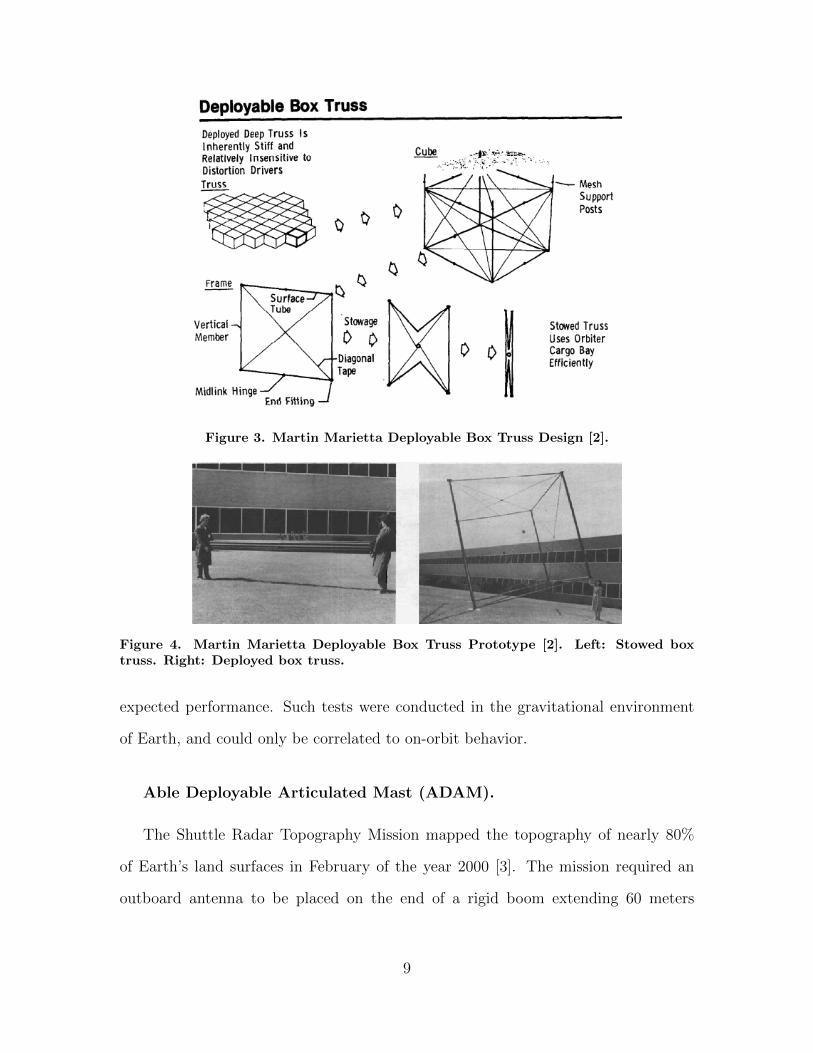
Figure 3. Martin Marietta Deployable Box Truss Design [2].
Figure 4. Martin Marietta Deployable Box Truss Prototype [2]. Left: Stowed boxtruss. Right: Deployed box truss.
expected performance. Such tests were conducted in the gravitational environment
of Earth, and could only be correlated to on-orbit behavior.
Able Deployable Articulated Mast (ADAM).
The Shuttle Radar Topography Mission mapped the topography of nearly 80%
of Earth’s land surfaces in February of the year 2000 [3]. The mission required an
outboard antenna to be placed on the end of a rigid boom extending 60 meters
9

from the shuttle itself. The ADAM (Able Deployable Articulated Mast) was a truss
structure consisting of 87 cube-shaped truss cells that not only held the outboard
antenna at a precise location, but could also retract back into the shuttle after the
mission.
Figure 5. ADAM deployed from canister in laboratory environment with gravity of-floading [3].
Today, the design and manufacture of this deployable mast is done by ATK
Aerospace Structures [14]. Unlike the Martin Marietta design, the box truss mem-
bers do not fold themselves. Rather, the members have ball joints on their ends to
allow the specialized corner fittings to fold the members as the box truss is rotated
in a deployment canister. Figure 6 shows a stowed 10 meter ADAM that was used
most recently for the NuSTAR mission in 2012 performed by JPL (Jet Propulsion
Laboratory) and the California Institute of Technology [4]. To date, ATK has flown
11 of these masts and has had a 100% success rate [14].
ATK lists some important advantages of using deployable truss systems for space
operations: high deployment reliability and repeatability, extensive flight heritage,
10

Figure 6. NuSTAR ADAM in stowed configuration [4].
validated on-orbit strength and stiffness performance, efficient stowage volume (< 5%
of total length), and a modular design that allows the mast length to be tailored for
specific mission requirements. However, this modularity only extends the length of
the mast and does not allow for additional truss cells in any other direction, unlike the
Martin Marietta concepts. Packaging efficiency is also not great, as Figure 6 shows a
considerable amount of unused space in the deployment canister.
Large Deployable Sparse Aperture Reflector Structural Design.
The Martin Marietta box truss cube showed significant promise. It had great
packaging efficiency, had multi-directional modularity, and was very strong. Unfortu-
nately, further design iterations were hampered by limited resources and applications
for the trusses. Very few prototypes were tested. The ADAM, on the other hand, is a
multi-joint, deployable truss structure with great flight heritage that has been proven
to be a viable solution for creating large structures in space. The thought then, is to
11

combine the best aspects of each design into a new large deployable space structure.
Enter the Large Deployable Sparse Aperture Reflector design that is currently being
investigated by the Air Force Institute of Technology (AFIT).
Figure 7. Conceptual side layout view of Large Deployable Sparse Aperture Reflector.Courtesy of Dr. Gyula Greschik [5].
The Large Deployable Sparse Aperture Reflector concept (Figure 7) was conceived
as a means to recreate the area of a 50 meter diameter filled reflector aperture with a
sparse design that could be stowed into existing payload fairings of approximately 5
meters in diameter. The reflector is intended to be used on a satellite in a geostation-
ary orbit and receives L-Band signals of 1-2 GHz [15]. Much work as been done to
down-select the design [10], increase packaging efficiency [10], calculate its electrical
performance [15], and determine the required manufacturing accuracy requirements
[12]. This work focuses on the deployment of the design chosen as a result of these
previous works.
In essence, the sparse aperture reflector is comprised of four arms which deploy
from a central hub (Figure 8). The arms are made from eight box trusses each,
henceforth known as truss cells, that are shaped into a parabola. The parabola is
created through the use of shaping tension cables on the sides of the cells as well
as unequal length top and bottom members of the truss cells. Additional structural
12

Figure 8. Top view of sparse aperture with 150 meter diameter compared to a filledaperture with 50 meter diameter. Courtesy of Dr. Gyula Greschik [5].
cables reside in the top and bottom faces of the cells as well, and serve to add more
rigidity to the truss cell. The deployment occurs in two stages: a bounded horizontal
opening of the truss cells via a motor in the hub (first stage), and an unbounded radial
expansion along the lengths of the truss cells (second stage). These stages are shown
in Figure 9 which is a more detailed representation of the geometry shown in Figure
8. The first stage of deployment unfolds the “horizontal battens” of the truss cell,
and the second stage of deployment unfolds the “longerons,” or the members that run
the radial length of the truss cell. Both the horizontal battens and the longerons are
split by hinges that lock after 180 degrees of rotation, but only the longeron’s hinges
contain a pre-deformed spring that motivates the radial deployment. The upright
structural members of the truss are known as vertical battens, and are static in their
length. Please refer to Figure 10 for an illustration of these structural members. Once
fully deployed, the entire structure is held in tension by the multitude of cables within
each cell as well as many other cables spanning different arms and the central mast.
The advantages of the Large Deployable Sparse Aperture Reflector concept are
numerous. Through the use of truss cells with tension cables, the reflector will have a
high stiffness to mass ratio similar to the Martin Marietta design. By collapsing
13
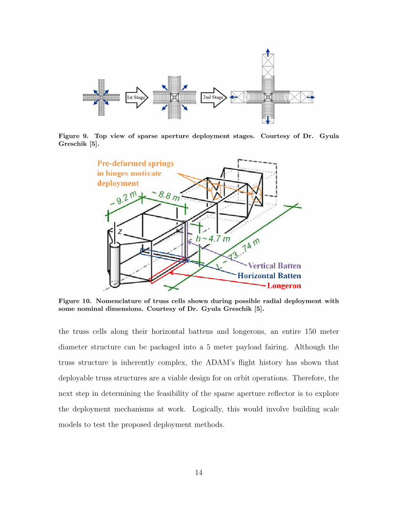
Figure 9. Top view of sparse aperture deployment stages. Courtesy of Dr. GyulaGreschik [5].
Figure 10. Nomenclature of truss cells shown during possible radial deployment withsome nominal dimensions. Courtesy of Dr. Gyula Greschik [5].
the truss cells along their horizontal battens and longerons, an entire 150 meter
diameter structure can be packaged into a 5 meter payload fairing. Although the
truss structure is inherently complex, the ADAM’s flight history has shown that
deployable truss structures are a viable design for on orbit operations. Therefore, the
next step in determining the feasibility of the sparse aperture reflector is to explore
the deployment mechanisms at work. Logically, this would involve building scale
models to test the proposed deployment methods.
14

High-Fidelity Gravity Offloading System.
The fabrication and test of proposed designs are critical to the development of
new technologies. Space structures require special consideration because they are
sometimes designed for a weightless environment. Measures need to be taken to
“offload” the structures so that the tests done to them are representative of the
space environment. Unfortunately, “ground tests to explore the zero-g performance
of mechanical systems inevitably employ various compromised solutions” [11]. Such
solutions usually involve hanging the structure so that it does not have to support its
own weight (Figure 5), or free-fall drop tests in which the subject is virtually weightless
for a short amount of time. For kinematic testing, more creative offloading schemes
must be devised so that the motion of the structure remains unimpeded by both
gravity and the offloading hardware itself [16]. Although many viable solutions for
gravity offloading exist and have been proposed, the fact remains that fabricating and
testing the hardware would be time-consuming and expensive. Most likely the design
under review in this work would at first be scaled to test the structure’s deployment
validity. Eventually though, a full-scale test to certify the structure for flight would
have to be conducted, which would require an enormous test facility. Fortunately,
modern computers and certain mathematical methods can be employed to conduct
analysis on large space mechanisms before they ever need to be fabricated. This
allows the designers of such large structures to test and iterate their designs many
times before the expensive full-scale fabrication and testing need to occur.
15

2.2 Static Finite Element Methods
Finite Element Analysis.
“FEA (Finite Element Analysis), also called the FEM (Finite Element Method), is
a numerical method to finding the solution to field equations” [7]. The field equations
spatially subdivide the whole domain of a problem into simpler, finite parts. Solving
for the dependent variables present in the field equations in a piece-wise fashion for the
whole domain yields an approximation of the exact solution. The exact solution itself
would almost certainly be impossible to solve for save the simplest of problems. Such
methods are extremely useful for solving complex problems and have applications in
a myriad of scientific fields. In particular, this work explores how FEM can be used
to simulate the deployments of space structures.
The foundation of finite elements lies in the discretization of geometry into “el-
ements.” These elements are connected at points known as “nodes” where the field
equations are applied and the dependent variables solved for. When dealing with
structural analysis, the nodal applications usually involve the material properties of
the geometry being segmented as well as the individual node’s local displacement.
The local displacements are commonly labeled as follows: u (Local X-Displacement),
v (Local Y-Displacement), and w (Local Z-Displacement). Interpolating these prop-
erties and displacements is done along the elements, and can be done with different
polynomial orders. The combination of multiple nodes and elements to describe a
geometry is known as a “mesh”. Figure 11 shows a simple 2D beam mesh in which
the three nodes are free to rotate and translate vertically, and are connected by two
elements.
Mathematically, the static finite element problem is represented as a system of
equations: [K] {D} = {R}. Here, the matrix [K] is the assemblage of the elements’
stiffnesses that are derived from the material properties of the geometry in question.
16
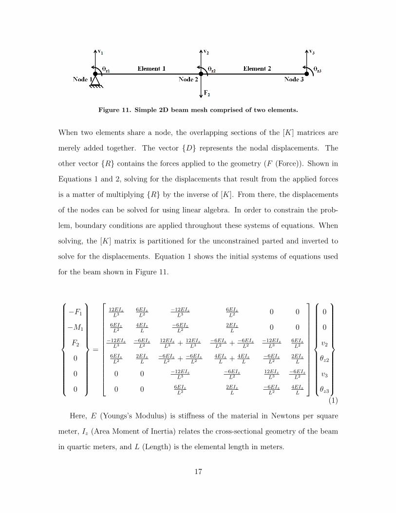
Figure 11. Simple 2D beam mesh comprised of two elements.
When two elements share a node, the overlapping sections of the [K] matrices are
merely added together. The vector {D} represents the nodal displacements. The
other vector {R} contains the forces applied to the geometry (F (Force)). Shown in
Equations 1 and 2, solving for the displacements that result from the applied forces
is a matter of multiplying {R} by the inverse of [K]. From there, the displacements
of the nodes can be solved for using linear algebra. In order to constrain the prob-
lem, boundary conditions are applied throughout these systems of equations. When
solving, the [K] matrix is partitioned for the unconstrained parted and inverted to
solve for the displacements. Equation 1 shows the initial systems of equations used
for the beam shown in Figure 11.
−F1
−M1
F2
0
0
0
=
12EIzL3
6EIzL2
−12EIzL3
6EIzL2 0 0
6EIzL2
4EIzL
−6EIzL2
2EIzL
0 0
−12EIzL3
−6EIzL2
12EIzL3 + 12EIz
L3−6EIzL2 + −6EIz
L2−12EIzL3
6EIzL2
6EIzL2
2EIzL
−6EIzL2 + −6EIz
L24EIzL
+ 4EIzL
−6EIzL2
2EIzL
0 0 −12EIzL3
−6EIzL2
12EIzL3
−6EIzL2
0 0 6EIzL2
2EIzL
−6EIzL2
4EIzL
0
0
v2
θz2
v3
θz3
(1)
Here, E (Youngs’s Modulus) is stiffness of the material in Newtons per square
meter, Iz (Area Moment of Inertia) relates the cross-sectional geometry of the beam
in quartic meters, and L (Length) is the elemental length in meters.
17
After applying the boundary conditions, the rows and columns of the DOF (De-
grees of Freedom) that were constrained are removed. Then, the forces vector is
multiplied by the inverse of the stiffness matrix to solve for the displacements and
create a solution for the problem.
v2
θz2
v3
θz3
=
12EIzL3 + 12EIz
L3−6EIzL2 + −6EIz
L2−12EIzL3
6EIzL2
−6EIzL2 + −6EIz
L24EIzL
+ 4EIzL
−6EIzL2
2EIzL
−12EIzL3
−6EIzL2
12EIzL3
−6EIzL2
6EIzL2
2EIzL
−6EIzL2
4EIzL
−1
F2
0
0
0
(2)
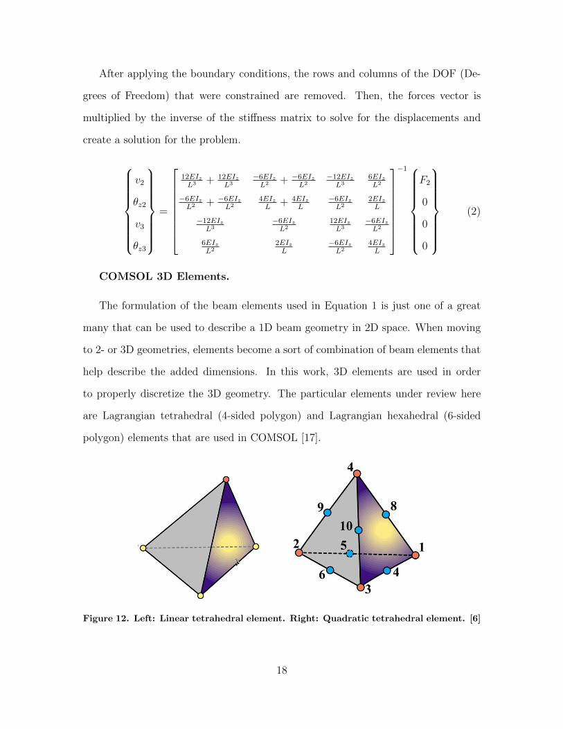
COMSOL 3D Elements.
The formulation of the beam elements used in Equation 1 is just one of a great
many that can be used to describe a 1D beam geometry in 2D space. When moving
to 2- or 3D geometries, elements become a sort of combination of beam elements that
help describe the added dimensions. In this work, 3D elements are used in order
to properly discretize the 3D geometry. The particular elements under review here
are Lagrangian tetrahedral (4-sided polygon) and Lagrangian hexahedral (6-sided
polygon) elements that are used in COMSOL [17].
Figure 12. Left: Linear tetrahedral element. Right: Quadratic tetrahedral element. [6]
18

By default, COMSOL meshes geometries with tetrahedrons. Tetrahedrons are
useful for meshing because almost any geometry can be approximated to arbitrary
precision with a sufficiently dense tetrahedral mesh. COMSOL even features an
‘adaptive meshing” tool that will coarsen or refine a meshduring a simulation in
response to certain convergence criteria at every time step. Figure 12 shows both
a linear tetrahedral element as well as a quadratic tetrahedral element1 The linear
tetrahedral element has 4 nodes, and the quadratic tetrahedral element has 10 nodes.
With 3 DOF per node, this gives the linear element 12 DOF and the quadratic element
30 DOF.
Figure 13. Left: Linear hexahedral element. Right: Quadratic hexahedral element. [6]
Although tetrahedrons can be used for many geometries, they are not always the
most efficient method for meshing. For certain geometries, especially certain simpli-
fied 3D trusses, hexahedrons are more effective. In COMSOL, hexahedrons require
extra effort from the engineer since they are not automatically meshed. Fortunately,
the mesh process is quite swift. Figure 13 shows both a linear hexahedral element as
well as a quadratic hexahedral element. The linear element has 8 nodes and 24 DOF
(3 DOF per node). The quadratic element has 20 nodes and 60 DOF (3 DOF per
node).
1The use of the terms ‘linear” and ‘quadratic” are elaborated in the following section.
19

Element Interpolation.
An important aspect of finite elements is the interpolation between the nodes of the
mesh. The formulations for the interpolation methods are numerous, and stem from
the “shape function” on which they are based. These shape functions are generally
classified by the order of interpolation they can provide between the major nodes.
For instance, a first order element can only interpolate linearly between two nodes. A
second order element places a secondary node between two primary nodes, and thus
allows for quadratic interpolation. In most cases, adding in these extra nodes allows
the element to approximate the “true” solution even better. As a consequence, the
total DOF of a mesh of quadratic elements will have a sizable increase. The system
stiffness matrix [K] will also be more densely populated. Both of these factors will
greatly penalize the simulation times. However, the mesh resolution could also be
lowered when using quadratic elements and reduce the size of the stiffness matrix
and the simulation time. At the end of the day, it is up to engineer to decide how to
balance the element order and mesh density when building a FEM model.
Figure 14. Left: Deformation mode of a rectangular block of material in pure bending.Right: Deformation mode of the Q4 element under bending load. [7]
Figure 14 is a simplified 2D case of when a higher order element is needed. The
Q4 (Four-node Bilinear Rectangle Element) on the right cannot exhibit pure bend-
ing. “When bent, it displays shear strain as well as the expected bending strain.
20

This parasitic shear absorbs strain energy, so that if a given bending deformation is
prescribed, the bending moment needed to produce it is larger than the correct value.
In other words, the Q4 element exhibits shear locking behavior” [7]. In short, the
use of linear elements such as the Q4 in a mesh under a bending load will cause the
stiffness of the mesh to be egregiously high. This elemental defect can be overcome
through the use of a higher order element. In this case, a Q8 (Eight-node Quadratic
Rectangle Element) with mid-side nodes would enable the sides of the element to
form a curve and correctly transfer the bending moment through the entire mesh.
This logic can be applied to 3D elements and meshes, such as the elements described
in the previous section.
2.3 Dynamic Finite Element Methods
Theory.
Many methods for structural dynamics were developed before the advent of FEM
for use on structures and so the calculation methods are largely independent. Today,
however, many methods have been tailored to fit the discretization of FEM models.
These methods not only use the same stiffness matrix found in static FEM, but also
require mass and damping matrices. Together, the matrices can be applied to the
solve for Newton’s second law as seen in Equation 3 [7].
f = ma⇒ r − ku− cu = mu⇒ mu+ cu+ ku = r (3)
where m (Mass), r (Forcing Function), a (Acceleration), k (Stiffness Constant), c
(Damping Constant), u (Velocity), and u (Acceleration). Note that the resulting
force of the spring ku may be called an internal force [7].
From this equation and some FE theory, the global form of Newton’s second law
21

for FEA can be written as Equation 4 or Equation 5 [7].
[M ] {D}+ [C] {D}+ {Rint} = {Rext} (4)
[M ] {D}+ [C] {D}+ [K] {D} = {Rext} (5)
where the capital letters indicate the matrix or vector form of their lower case coun-
terparts to show that these are discretized sample locations. Also note that matrices
are represented by brackets and vectors are represented by braces.
Explicit and Implicit Integration Methods.
There are two basic methods of integration used to solve these equations: explicit
and implicit. Both have their own advantages and disadvantages, but the main goal
of these methods is to solve for the displacement {D} of the system for one time step.
Explicit direct integration is a conditionally stable form of numerical integration
that requires both the knowledge of the past and present to compute the solution to
the future. It is best suited towards “wave propagation” type problems. The stability
of this method hinges upon the time step chosen, which is a function of the structure’s
mass and stiffness. Usually, the time step chosen must be very small to yield a stable
result, meaning that the solutions found with this method are often very exact at the
cost of a high amount of time steps needed. Thankfully these steps are usually cheap
in terms of computation time because the matrices are diagonal. Shown here as an
example is the “Half-Step Central Difference” method in Equation 6.
1
∆t2[M ] {D}n+1 =
{Rext
}n−{Rint
}n+
[2
∆t2M − 1
∆tC
]{D}n−
[1
∆t2M − 1
∆tC
]{D}n−1
(6)
22

The time step (∆t (Time Step)) is limited by the resonance of the highest fre-
quency component, which generally corresponds to the smaller elements used for
detailing the structure. For highly detailed structures, it becomes quite difficult to
find a stable time step with explicit methods. It is therefore more advantageous to
use implicit methods whose accuracy, not stability, depend on the time step used.
Implicit methods only require knowledge of the present to compute the solution to
the future. This allows most methods to be unconditionally stable and is more useful
for structural dynamics. The biggest downside to this possible unconditional stability
is the amount of computation it takes to solve for the non-diagonal matrices in the
problem. For this particular example, the numerically stable Newmark Method is
used and is shown in Equation 7.
[Keff ] {D}n+1 ={Rext
}n+1
+[M ]
{1
β∆t2{D}n +
1
β∆t
{D}n
+
(1
2β− 1
){D}n
}+ [C]
{γ
β∆t{D}n +
(γ
β− 1
){D}n
+
(γ
2β− 1
){D}n
}(7)
Where γ (Gamma) and β (Beta) are numerical factors that control characteris-
tics of the Newmark Method such as accuracy, numerical stability, and algorithmic
damping.
Previous work [8] with these methods show systems that can be precisely charac-
terized are best represented with explicit methods. However, for systems that cannot
be fully characterized, only the implicit methods yield converging2 results easily.
As an example, take a cantilevered beam similar to that of the problem detailed in
Figure 11 with an impulsive load is applied along its length at the free end. Figure 15
shows how the stress in the middle of the beam increases as a stress wave propagates
2Convergence here meaning that the algorithm is stable enough to find a solution within settolerances.
23

through it3. The explicit results are more intuitively representative of the stress wave
propagation while the implicit results are filled with noise. Yet, these explicit results
are gained from a precisely calibrated time step. Figure 16 shows what happens if
this time step is altered by just one nanosecond. The COMSOL results shown are
different dimensional representations of the same beam that were run for the sake
of comparison. Plainly, this kind of instability is not conducive for a system more
complex than the simple cantilevered beam shown here. It is for this reason that
the implicit solvers4 within COMSOL were chosen to compute the solution to the
deploying trusses in which the final solution is relatively unknown. Figure 17 shows
that COMSOL’s implicit solver fares very well in various dimensions against the
aforementioned numerical methods and thus validates COMSOL’s implicit solver for
this scenario.
Figure 15. Axially-loaded cantilevered beam: explicit vs. implicit methods. [8]
3Note that the simulation time is only for 0.3 milliseconds in order to view the stress wave’spropagation.
4The implicit solver used in COMSOL is described in detail in Section 2.3.
24

Figure 16. Axially-loaded cantilevered beam: explicit method deviation due to timestep variance. [8]
Figure 17. Axially-loaded cantilevered beam: COMSOL vs. explicit and implicit meth-ods. [8]
25
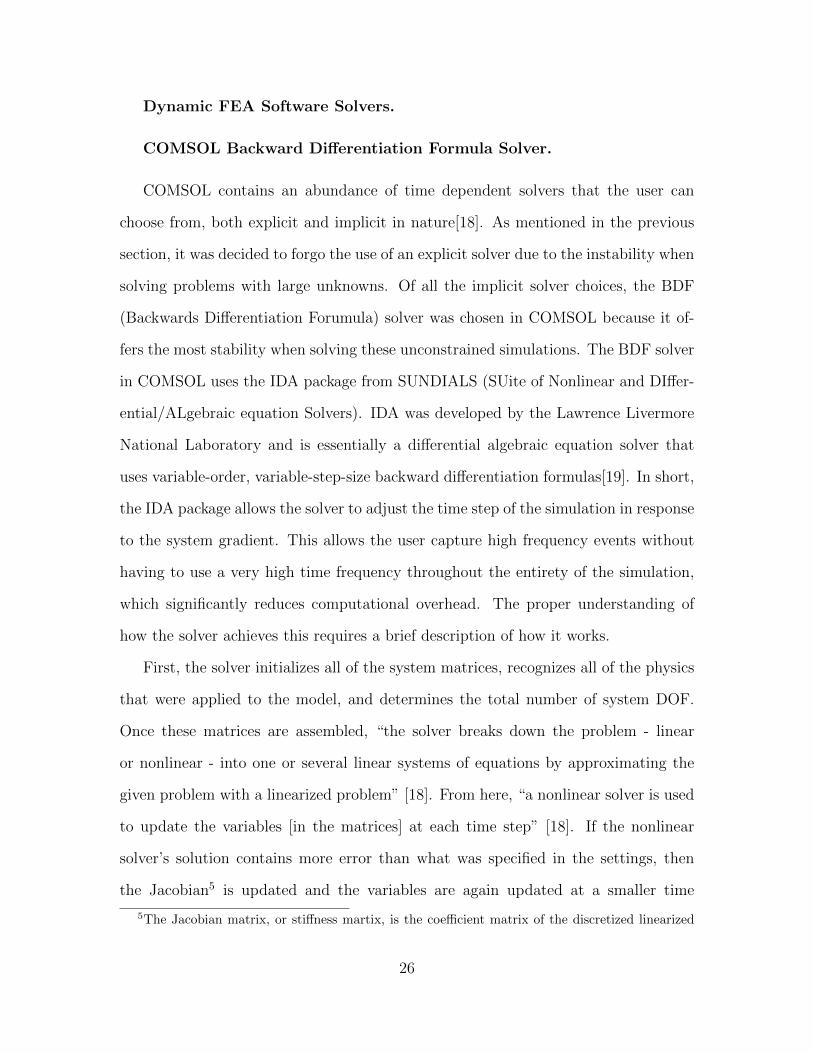
Dynamic FEA Software Solvers.
COMSOL Backward Differentiation Formula Solver.
COMSOL contains an abundance of time dependent solvers that the user can
choose from, both explicit and implicit in nature[18]. As mentioned in the previous
section, it was decided to forgo the use of an explicit solver due to the instability when
solving problems with large unknowns. Of all the implicit solver choices, the BDF
(Backwards Differentiation Forumula) solver was chosen in COMSOL because it of-
fers the most stability when solving these unconstrained simulations. The BDF solver
in COMSOL uses the IDA package from SUNDIALS (SUite of Nonlinear and DIffer-
ential/ALgebraic equation Solvers). IDA was developed by the Lawrence Livermore
National Laboratory and is essentially a differential algebraic equation solver that
uses variable-order, variable-step-size backward differentiation formulas[19]. In short,
the IDA package allows the solver to adjust the time step of the simulation in response
to the system gradient. This allows the user capture high frequency events without
having to use a very high time frequency throughout the entirety of the simulation,
which significantly reduces computational overhead. The proper understanding of
how the solver achieves this requires a brief description of how it works.
First, the solver initializes all of the system matrices, recognizes all of the physics
that were applied to the model, and determines the total number of system DOF.
Once these matrices are assembled, “the solver breaks down the problem - linear
or nonlinear - into one or several linear systems of equations by approximating the
given problem with a linearized problem” [18]. From here, “a nonlinear solver is used
to update the variables [in the matrices] at each time step” [18]. If the nonlinear
solver’s solution contains more error than what was specified in the settings, then
the Jacobian5 is updated and the variables are again updated at a smaller time
5The Jacobian matrix, or stiffness martix, is the coefficient matrix of the discretized linearized
26
step6. Error is usually a result of the system becoming more dynamic through high
acceleration and usually correlates to high stress events. The iterations continue until
the error is small enough to satisfy the settings, and then the step is written out for
that time interval. The iterative method also works in reverse: if the nonlinear solver’s
solution has very small error, then the solver will strive to increase the time step to
its maximum allowable amount in order to speed up the total computation time.
To illustrate this point, Figure 18 shows the longeron stresses at the top and time
step reciprocal at the bottom from an early two cell truss deployment simulation.
Note that both plots are matched up despite their different X axes. Following the
annotations present in the figure: Event 1 marks the start of the deployment when
the spring-hinges applied their moment to the longerons. Although the stress is not
high here, a lot of rapid acceleration occurs as the applied moments begin to move
the truss cells. After the mechanism “settles” to a steady state, the time steps return
to the default level of 0.01 seconds. Event 2 marks the locking hinges for the first
truss cell to fully deploy. The first peak is the upper longerons and the second peak is
the lower longerons. Note that the spikes in time steps cover a period of time before
and after the locking occurs. Smaller time steps are needed here because the system
is rapidly changing as the longerons accelerate towards their peak velocity. After the
locking event, the time steps remain small for a time while the stress is dissipated.
Event 3 marks the locking event in the second trusses lower longerons. The upper
longerons failed to deploy before the simulation ended. Again, the time steps needed
to capture the stress event are small, yet they are allowed to become larger once the
system reaches a steadier state and the stress waves dissipate below the tolerances
set.
problem. Although it does not necessarily have to be updated for every iteration, the problem isquicker to converge if it is.
6COMSOL is also wont to try a higher order approximation here to gain more accurate results,however this occurs much more infrequently.
27

Figure 18. Top: Longeron stresses during two truss deployment simulation with respectto time. Bottom: Reciprocal of the time steps used during the simulation with respectto time steps.
28

Figure 19. Example of the reciprocal time steps during a simulation for a poorly mademodel.
On a final note, it should be mentioned that the reciprocal time step plot is also
very useful in determining the health of an ongoing simulation. All too often a model
will not be set up correctly or is meshed poorly and the time steps needed for a
converged solution become quite microscopic. Figure 19 is an example of a model
that is not stable during certain movements of its deployment. By reviewing the
results from this simulation during the instances where a time step of 1 picosecond
was needed, one can attempt to “debug” the model. Many times spikes such as these
are indicative of an error in the modeling, but some times the model may need to be
adjusted by adding damping or loosening some of its constraints.
2.4 Computational Hardware Concerns
Throughout the course of developing this work - configuring models, creating
meshes, testing solver settings, etc - it became apparent that the computer hardware
being used would significantly affect the pace of the work being done for this thesis.
As the models became larger with added complexity, not only would a more powerful
computer enable the simulations to finish sooner, but the user would be able to
29

iterate upon the design at a faster pace if multiple instances of COMSOL could be
used simultaneously. It then became a secondary objective to explore some different
hardware options to potentially improve this work’s throughput. COMSOL itself has
many suggestions to improve simulation performance with hardware [20], chief among
them is the memory bandwidth. As most of COMSOL’s solver algorithms are multi-
threaded and can be spread around to available processor cores, the amount and speed
of the memory channels feeding into the cores is of utmost importance. In this way
the computer can assemble the system matrices in memory, shuttle the information
to the processor for computation, and then read the computed information back into
memory, as fast as possible. In addition to COMSOL’s suggestions, there exists a
plethora of anecdotal information of other user’s experiences online. Many users
found that increased processor clock speed as well as server-grade hardware (multiple
processors) considerably reduced simulation time. Table 1 offers some anecdotal
information encountered during the development of this work.
Table 1. Computer Simulation Benchmark
Computer Desktop LaptopProcessor Quad Core 4.2 Ghz Quad Core 2.3 GhzMemory 16 GB @ 2133 MHz 8 GB @ 1600 MHz
Memory Channels 4 2Peak Processor Temperature 47◦C 86◦C
Simulation Time (1 Cell) 21m 41s 28m 48sSimulation Time (4 Cells) 4hr 17m 28s 5hr 49m 30s
The first computer that was used in the early stages of this work’s development was
the laptop. For a laptop, it is very powerful and features a quad core processor and
workstation graphics card. However, the memory provided little overhead for bigger
simulations and its cooling system did not cope well with the processor’s thermal
load. The simulation time for a single cell truss deployment was respectable, but for
a four cell truss the laptop would have to push itself for almost six straight hours.
30

For the sake of comparison, the same simulations were run on a desktop computer.
The desktop has a newer quad core processor that is overclocked and has twice the
available memory channels as the laptop. More importantly, the desktop’s memory is
25% faster than that of the laptop, enabling the both simulations to run approximately
25% faster. Although this direct correlation is dubious, it cannot be denied that
running a four cell truss simulation in 4 hours, 17 minutes is much better than 5
hours and 49 minutes. For larger simulations, the time differences will most likely
scale so that a simulation that might take four days could be instead accomplished in
three. Not to mention the additional memory overhead of the desktop allows the user
to run multiple instances of COMSOL simultaneously and at much safer processor
temperatures.
A 25% increase is a good gain from moving from the laptop to the desktop,
but one could posit that the increased speeds gained from the desktop should be
even greater. After all, the desktop has twice the number of memory channels and
almost twice the processor clock speed. There are two specific factors that refute
this conjecture. First, while the simulations still take a considerable amount of time,
they are still considered small with “only” 20,000 DOF. The benefits of more memory
bandwidth and higher clock speed may not be apparent until the model’s matrices
are big enough to take advantage of it. Second, the specific solver being used here
may not be completely optimized for parallelization. Amdahl’s Law states that the
expected improvement of a parallel computing system is a function of the percentage
of parallelized threads [21]. Meaning that if a portion of an algorithm is serialized,
then the minimum execution time of the algorithm cannot be less than that of the
serial process. Therefore, COMSOL’s partially parallelized algorithms will not be
sped up as a function of cores added and is instead at the mercy of the slowest serial
process.
31

2.5 Summary
Section 2.1 started by showing an overview of the work done on the Martin Ma-
rietta deployable space truss and ATK’s ADAM. These subsections show that while
the deployable space truss was ingenious, the lack of available applications at the
time prevented it from being iterated further. ATK’s ADAM proved that large de-
ployable space trusses with a multitude of joints can indeed be successful in space,
but that perhaps more efficient packaging could enable even larger space structures.
The next subsection explained how the Large Deployable Sparse Aperture Reflector
borrowed some of the best ideas from the aforementioned historical works, and put
them to use to design a new breed of antenna reflector. The final subsection here
then briefly talked about the challenges of testing space structures on Earth, and how
testing the designs computationally is a viable, cost-effective alternative to the classic
design-fabricate-test-review cycle. Section 2.2 first covered the basics of the Finite
Element Method through the use of a simple example. These basics were then pushed
further to show how FEM can be used to solve for different 3D geometries with dif-
ferent types of elements. It then stressed the importance of higher order elements
and how the can more accurately describe the behavior of structures under bending
loads. Section 2.3 showed how explicit and implicit methods can be applied to solve
dynamic FEA problems. It was stated that although explicit methods are the most
accurate, they require a system characterization that could not be properly made
from the relatively unknown deployment of the locking space trusses. The section
finished by describing the techniques being used by COMSOL to solve its simulations
implicitly. COMSOL’s method of varying the solver’s time step in response to system
gradients was also outlined with an accompanying example simulation. Finally, some
computation considerations were voiced to show how different hardware affects the
simulation time. It was found that for these simulations, the main contributor to
32

reduce simulation time was most likely the computer’s memory speed. A note was
also made to state that computer hardware scaling is not trivial, and is extremely
reliant on the parallelization of the software code.
33

III. Methodology
Chapter 3 explains the methodology used to simulate the truss deployment of the
Large Deployable Sparse Aperture Reflector concept described in the previous chap-
ter. It begins in Section 3.1 which details why COMSOL was the FEA software of
choice for this work. Next, Section 3.2 illustrates the 3D modeling of the trusses in
Solidworks to show how the trusses are stowed and deployed. This geometry is simpli-
fied in the following section so that the simulations can focus more on the deployment
behavior and less on the individual components that constitute the structure. Due
to the simplification, the as-designed material properties are adjusted in Section 3.3.
Section 3.4 then introduces the nomenclature that was created as a shorthand and
is used to called out the different aspects of the model throughout this work. After
this preparation, the model is imported into COMSOL in Section 3.5. Here the entire
process of composing the simulation in COMSOL is detailed from importing the ge-
ometry to entering the correct solver settings. Subsection 3.5 is of particular interest
and describes the method in which the cable “elements” were created. Section 3.6
explains how a meshing study was done in COMSOL to determine the most efficient
meshing strategy for the simulations. The study aims to create a mesh that is both
accurate and computationally inexpensive. Section 3.7 is the final section in Chapter
3 and describes how the deployment envelope of the simulation can be calculated
from the results of COMSOL in MATLAB.
3.1 FEA Software Selection
One of the first steps in this work was to select the FEA software package that
would run the truss deployment simulations. Five different commercial packages
were vetted in order to determine their capabilities, specifically their ability to model
34

multibody dynamics. It was also important that these packages be able to use flex-
ible bodies, handle large amounts of data, and have in-depth documentation. The
following subsections briefly discuss the different packages that were explored, and
why they were not chosen over COMSOL.
FEMAP.
FEMAP (Finite Element Modeling And Postprocessing) is a FEA program that
excels at static FEA problems. It is extremely configurable, and allows the user to
change almost every aspect of the model. Unfortunately, FEMAP is not built for
multibody dynamics, and is generally used only to create the meshes for multibody
dynamic simulations. To run these simulations, the meshes would have to be imported
into a partnered program such as MSC ADAMS.
MSC ADAMS.
ADAMS (Automated Dynamic Analysis of Mechanical Systems) is a software
package that excels at multibody dynamics simulations. In general, ADAMS is an
industry standard package that can provide high fidelity simulations of mechanical
mechanisms. It accepts many different types of meshes and can even use beam ele-
ments in place of solid bodies, unlike COMSOL. However, the types of motions that
would be expected for the deploying truss did not align very well with the ADAMS’
toolkit. Through testing done with an educational version of ADAMS, it was found
that the motion constraints of a simulation are largely predicated on the geometry
being used. For a locking hinge truss, it appeared as though the geometry would
have to be built to physically stop and lock the hinges. This was not optimal for
simulations that were being run to explore the global deployment of a large structure.
Additionally, ADAMS did not seem to have much control over the meshes, and would
35
rely on a secondary software package. This would not be ideal if the mesh needed
to be iterated quickly. Therefore it was decided that although ADAMS would most
likely be a fit for this work, it might take a large amount of effort to properly model
the locking truss.
Abaqus.
Abaqus was the software of choice used in the second Finite Elements course at
AFIT. Throughout this course it was shown that Abaqus allows the user a great
amount of control over the model, and that accurate results could be had with the
large library of elements available. In fact, Abaqus is very popular with major auto
manufacturers, who use it to simulate crash tests. However, during conversations
with faculty at AFIT who were extremely familiar with Abaqus, it was decided that
Abaqus would not be a good fit for simulating the deploying truss. It was advised
that a large amount of work would needed in a supporting program such as MATLAB
in order to properly model relative motion inside of Abaqus. It was suggested that it
would be wiser to seek another FEA program for the deployment simulations.
Recurdyn.
Recrdyn is a relatively new FEA program that offers a promising multibody dy-
namics package. It is currently being used extensively by Asian automotive manu-
facturers and even includes special tool kits for automotive simulations. It is also
listed as a complementary software to ANSYS [22], which is a FEA program with
great heritage. A full version of the software was obtained and tested. The user
interface for Recurdyn was simply laid out and easy to understand. It allowed the
user to easily build rigid 3D models, declare joints between bodies, and plot results
very quickly. However, the software still had some of the same issues as ADAMS. It
36
was geared towards finalized geometries, had very little control over the meshes, and
custom functions would have to be built to create the appropriate mechanisms for
locking the trusses. Despite these issues, Recurdyn was used to create an extended
abstract on locking hinge truss deployments for the 2015 AIAA SciTech conference.
This extended abstract precedes the conference paper, which in turn precedes this
very thesis. Through this process it was discovered that although Recurdyn models
simplified rigid bodies very well, custom locking parameters had to be created to
in order to stop the bodies without geometry. Before continuing the work for the
conference paper, it was decided to explore another FEA program.
COMSOL.
COMSOL multiphysics is a FEA program that is built for simulations that in-
volve multiple physical interactions, such as a beam under bending and heating. At
first, one of the main attractions to COMSOL was its multibody dynamics package
that includes a large library of physics to create mechanisms. Importantly, spring,
dampers and locking attributes could be added to hinges which is not a convenient
task in ADAMS or Recurdyn. It was found that these hinges could be created quite
easily between faces of simplified geometries as well and did not require fully-realized
designs. Once COMSOL’s variable step solver was investigated and shown to save
valuable computation time, the decision to use COMSOL was almost certain. Unfor-
tunately, COMSOL’s multibody dynamics package used to simulate relative motions
demands the use of solid bodies to declare relationships between geometries. This
meant that the simulation sizes would be much larger than a FEA package that could
solve dynamics with simple beam elements. However, this drawback was accepted
because of all the choices, COMSOL appeared to offer the path of least resistance to
creating a locking truss simulation.
37

3.2 Geometry Modeling
3D Geometry Modeling.
The 3D geometry was created from 2D drawings from the work previously done
to design the truss [10]. The dimensions listed in the work were followed as closely as
possible. However, some dimensions have yet to be determined for the truss cells and
had to be estimated in order to create a reasonable representation of the geometry.
All modeling was done in Solidworks, which was chosen because of its availability and
familiarity to the author. Figure 20 illustrates how the 2D drawings were interpreted
to create the 3D geometry.
Figure 20. Left: 2D upper end fitting drawing (Courtesy of Dr. Gyula Greschik).Right: 3D upper end fitting model (angled view).
The ends of the longerons and battens were also modeled using the 2D drawings.
The hinges that split the longerons and horizontal battens have not yet been designed,
and are therefore omitted from the 3D models. Instead the longerons and horizontal
battens are spaced in order to allow for future design additions, and these spaces
38

along with the lengths of the members adhere to the nominal dimensions of the truss
cell. Figure 21 shows the stowed configuration of the truss cell and Figure 22 shows
the deployed configuration of the truss cell. Note that the view shown is of a nominal
“straight” cell, whereas the cells comprising the reflector are trapezoidal to create a
parabolic shape.
Figure 21. Left: Top view of 2D stowed configuration (Courtesy of Dr. GyulaGreschik). Right: Angled top view of 3D stowed configuration with some transparency.
Figure 22. Angled view of 3D deployed truss cell.
The nominal material properties of the as-designed geometry are shown in Table
2. Note that only one truss cell was modeled in this manner, and that additional
39

Table 2. Truss Member Material Properties
Young’s Modulus 70 GPaCoefficient of Thermal Expansion 7.4 mm/(m×K)Density 1600 kg/m3
Truss Diameter 51 mmTruss Wall Thickness 0.635 mmCable Diameter 3 mmCable Tension 10 N
truss cells would be added serially along the longeron direction. Each truss cell would
also be made from longerons of differing lengths top and bottom, varying cell to cell,
in order to create the final parabolic shape of the reflector.
3D Model Simplification.
As previously mentioned, the nominal geometries shown in the previous section
have not yet been finalized, and so it was decided that the geometry be simplified.
This not only allows for the simulations to focus more on the global deployment
of the trusses, but also considerably reduces the computational burden by requiring
less elements in the model to properly describe the geometry. Shown in Figure 23,
the 3D model was simplified into hexahedrons, which enables the geometry to be
discretized by either hexahedral or tetrahedral elements. The simplified geometry
was only modeled in the stowed configuration with the horizontal battens represented
as a solid member. This not only simplifies the model further, but also helps focus
the simulation on the second radial deployment.
Care was taken during the simplification process to make the simplified model very
easy to work with in COMSOL. The end fittings of the simplified geometry are shrunk
into blocks that allow for accessible hinge declarations on their edges. Consequently,
this also increases the visibility of the partially hidden lower longerons. Attached
to the back of each end fitting is a solid “bumper” that allows for contact to be
40

Figure 23. Left: As-designed geometry. Right: Simplified geometry with some trans-parency.
made between adjacent end fittings so that the geometry does not intersect during
the simulation1. The as-designed outer diameter of the longerons and battens is 51
millimeters and is designed so that there is very little gap between the longerons of
adjacent truss cells. The simplified geometry has a square cross section with an edge
length of 50 millimeters, to allow for more separation of the hexahedral boundaries
as well as reducing the chance of geometry intersection. Every truss cell was created
in its own SolidWorks assembly with an offset of its location in space relative to the
other truss cells when stowed. To create the reflector arm, these assemblies are merely
added together in a master Solidworks assembly. This modular approach allows the
simulations to be scaled by number of truss cells, and proves to be a boon when
1During the development of this methodology it was found that multiple cell simulations wouldcause the end fittings to intersect as one would be “kicked back” into another. Contact pairs adds aforce between the selected faces when they reach a predetermined spacing and were created on thebumpers to keep the end fittings and battens from intersecting.
41

investigating these deployment simulations in COMSOL. The entire simplified truss
is shown in Figure 24.
Figure 24. Simplified geometry of stowed four cell truss.
3.3 Equivalent Material Properties
Due to the simplification of the geometry, the material properties of the solid
hexahedrons were adjusted so that they behaved as the as-designed carbon fiber
tubes. This was simply done by using the geometric properties of the hexahedrons
and carbon fiber tubes in Equations 8 and 9 to create an equivalent Young’s Modulus
(E) and density (ρ).
42

Eadjusted =EcarbonfiberItube
Iblock(8)
ρadjusted =ρcarbonfiberVtube
Vblock(9)
Where E (Young’s Modulus), I (Second moment of area), ρ (Density), and V
(Volume).
These new values were then validated using Equations 10 and 11 [23][24]. The
validation equations were used with the parameters of a slender, simply supported
beam (Figure 25) that is analogous to a fully extended longeron.
Figure 25. Simply supported beam validation problem setup.
δmax =Pl3
48EI(10)
ωn =1
2π
(nπl
)2√EI
ρA(11)
Where P (Applied load), l (Length of beam), n (Natural frequency integer), and
A (Cross-sectional area).
Table 3 shows that the material properties of the carbon fiber tubes are carried
over exactly to those of the solid hexahedrons. However, it should be noted that this
conversion only works for bending modes of the longerons and is not valid for axial
loads. It will be shown later in this work that the members making up the truss cell
experience almost all bending loads during deployment, and that this equivalency is
43

Table 3. Adjusted material values: Constants and dependent values
Carbon Fiber Tube Adjusted Solid BlockSecond Moment Area of Inertia (I) 2.5973× 10⁻⁷ m 5.2083× 10⁻⁷ m
Young’s Modulus (E) 70 GPa 34.892 GPaDensity (ρ) 1600 kg/m3 32.3543 kg/m3
Max Displacement (δmax) 0.0982 m 0.0982 m1st Natural Frequency (ω1) 8.2517 Hz 8.2517 Hz
acceptable.
3.4 Modeling Nomenclature
A naming convention scheme was created in order to keep track of the various
hinges and forces within the COMSOL model as a shorthand code. Although this
system reduces clutter within the model, it does require some explanation. First
of all, it should be understood that the model is centered in space with the origin
in the center of square made from the end fittings, horizontal battens, and vertical
battens (Figure 26). In particular the vertical battens lie along Y direction while the
horizontal battens lie along X direction. The shorthand for the corners of the truss
cells is to merely state the positive or negative X and Y locations of the corner. For
example, “pxpy” indicates the positive X, positive Y corner of the truss cell. As the
longerons deploy outwards from the base square at Z = 0, they travel in the positive
Z-direction. This base square is known as the zeroth cell, represents the base of the
truss arm, and is a stationary reference frame. Moving in the positive Z-direction
from here, the truss cells are numbered 1, 2, 3, and 4, with the 4th truss cell being
the furthest out.
The joints within the cells are labeled according to their connections and spatial
position in the deployed truss state. Moving in the positive Z-direction, the joints
connecting the longerons to the frame square (and their shorthand) are: frame-to-
longeron (frlg), longeron-to-longeron (lglg), longeron-frame (lgfr). Therefore, a callout
44

Figure 26. Left: Spatial positioning of four cell truss. Right: Order of truss cell squares.
in the results for “c3.nxpy.lgfr” indicates the joint connecting the longeron member
to the square frame in truss cell 3 on the corner of negative X and positive Y. The
variable being viewed appends all of the nomenclature in the results section of this
paper. Meaning that “c2.pxny.lglg.Ms” is the Mapplied (Applied Spring-Moment) of
the longeron-to-longeron joint located in the positive X, negative Y corner. As a
special case, the cables follow these basic principles, and can be located in the model
by noticing last capitalized characters: “c1.NXnypy” signifies the cable that lies on
the negative X face that travels from (in the positive Z direction) the negative Y
corner to positive Y corner of the truss cell. Figure 27 shows a visual example of the
nomenclature applied to a truss cell and Figure 28 can be used as a reference guide
when viewing the results.
3.5 COMSOL Simulation Setup
The section presented here outlines a ”best practice” work flow for setting up
simulations in COMSOL. It is intended to show the advantages and disadvantages of
45

Figure 27. Truss cell 1 deployment at 7 seconds with hinge and cable callouts.
using COMSOL for multibody dynamic simulations. The methodology begins with
geometry import and conditioning, then moves through meshing, material properties
application, physics setup, cable modeling, probe creation, and finally solver config-
uration. All of these steps result in a model that can be varied and possibly run
systematically for parameter sweeps.
Geometry Import and Conditioning.
Importing geometry into COMSOL is a simple affair, requiring the user to select
which kind of files they are importing (COMSOL accepts a wide variety of CAD
files), and choosing which bodies or faces to import. The next step is to declare
graphically which imported bodies, or domains as they are called in COMSOL, are
solidly connected to one another. This is done with a ”Union” boolean function.
In Figure 29, the square comprising the horizontal battens, end fittings and vertical
battens were declared to be one domain, and the hinge attachment to the longerons
was also declared to be one domain with its adjacent longeron.
46

Figure 28. Legend for naming convention reference.
Meshing.
It is important to mesh the domains of the model that have been imported into
COMSOL before anything else to ensure that the 3D modeling and geometry condi-
tioning functioned as expected. An oversight in the settings of Soliworks can affect
how the mesh is applied to the domains where the various components meet. By
default, COMSOL automatically meshes the domains with tetrahedrons [18]. For
many applications a tetrahedral mesh may work well, but as will be seen in Section
3.6, it does not work for the slender components in use here. A hexahedral mesh
can be applied quite simply in COMSOL by selecting a face to map a quadratic grid
upon, and then “sweeping” this grid through the 3D domain. The number of edge
elements can be controlled by attaching a “distribution” sub-node and altering the
values. The truss cell was meshed in this manner with a different distribution setting
for the longerons, battens, and end fittings. Interestingly, the setting for the order
of the elements in COMSOL does not reside within the meshing node and is hidden
by default. It is instead found in the main physics node and can be adjusted from
1st (linear) order up to 4th (quartic) order. Figure 30 shows the meshed model,
please note that the lines perpendicular to the members are indicative of elemental
47

Figure 29. Left: Battens and end fittings declared as one domain. Right: Longeronand hinge attachment declared as one domain.
Table 4. Applied Material Properties
Longerons and Battens End FittingsYoung’s Modulus (E) 34.892 GPa 70 GPa
Density (ρ) 32.3543 kg/m3 1600 kg/m3
Poisson’s Ratio (ν) 0 0
boundaries. Section 3.6 will provide reasoning for the particular discretization shown.
Material Properties Application.
The material properties of the cell trusses are applied graphically to the geometric
bodies. The properties themselves are declared as simple materials: only applying
a Young’s Modulus, Poisson’s ratio, and density. All of the longerons and battens
are given the material properties from Section 3.3. The end fittings are given basic
properties of carbon fiber[25] because nominally they would be made from molded
composite material[10].
48

Figure 30. Rotated view of meshed model with end fittings closeup.
Physics Setup.
“Physics” nodes in COMSOL are sets of equations that are applied to selected
geometries within the model [18]. These equations determine the behavior of the ge-
ometry throughout the simulation. During the time spent creating the methodology
for the truss deployment simulations, it was found that COMSOL is usually more
agreeable to having lesser constrained models. Adding in possibly redundant con-
straints not only causes the solver to run slower because of the additional equations,
but also restricts the model to very few modes of movement and reduces the chance
of a converged solution.
At their most basic level, a physics node such as “Fixed Constraint” acts as a
boundary condition that locks a geometry face in a static position in space (u = v =
w = 0). The Fixed Constraint was applied to the bumper blocks of Cell 0, and is
the only constraint holding the deployment in place. The next step was to declare
49

the hinge joints of the mechanism. This was done by choosing two geometric faces as
attachments for the joint; one as the source and another as the destination. A hinge
joint was then created that uses both of these attachments with an axis declared on
a viable geometric edge. Figure 31 illustrates the main idea behind joint creation.
Within the hinge joint node are many options to give the joint extra properties.
For the hinges created between longerons (lglg), “Spring and Damper” as well as
“Locking” attributes are added. The hinges that join the back of the longeron to
the square frames (frlg), also have a constraint attribute that prevents the longerons
from rotating backwards. Next, forces were attached to the same hinge attachments
mentioned earlier to translate the cable force to the structure. Each cable exerts a
force on both of the attachments it is connected to, creating a tension force that
“squeezes” the truss cell. Finally, distinct contact boundaries were defined between
the front of each truss cell corner and the back of the “bumpers” on the next truss
cell. The contacts are set to use a “penalty” force between the two faces if a minimum
contact threshold is breached.
Figure 31. Example of joint being created between stowed longerons.
The order of the joint creation in this model was very important as it enhances
the overall modularity of the model. As mentioned earlier, the Solidworks model is a
50

modular design in which additional cells can be added one at a time. In COMSOL,
the same pattern was followed to declare each of the hinges in the cell before moving
on the the next. This makes calling out the same corner hinge from each cell very
easy, as they are all multiples of each other. The next section benefits tremendously
from this, as the files that determine the cable forces need only be adjusted slightly
to work with the next cell.
Cable Modeling.
Modeling cables in FEA programs is usually quite difficult due to their physical
behavior. Cables do not compress, and are referred to as “zero compression” elements
[26]. This behavior challenges a lot of FEA solvers because they must continually
check the direction of the cable force to determine whether that force is in tension
or compression. COMSOL does not have any cable physics nodes, but has a large
library of other types of joints with equations available for viewing. By studying
the equations that model different kinds of joints, a “cable-joint” was created. This
new pseudo-joint is a combination of a contact and distance joint. At its most basic
level, the distance between the two attachment faces is monitored until it reaches a
certain threshold. Once past, a force is applied between the attachments, just as a
cable would. If for some reason the distance between the attachments becomes less
than the unstretched length, then the force goes back to zero. Figure 32 shows the
equations of just one of the cables in the simulation, with explanations appearing in
the following paragraph.2
Note that these are text files that are imported into COMSOL, and do not have
numbers on the left column. The numbers are used for illustration purposes only.
When COMSOL does read in the file, however, the spaces between the strings of
2c1.NXnypy indicates the cable in Cell 1 that spans from the negative Y to positive Y corners(moving in the positive Z direction) on the negative X face of the cell.
51

Figure 32. Cable c1.NXnypy equation. Comments and line numbers added for clarifi-cation.
characters are separators to place the strings in adjacent columns. Therefore, the left
column states a variable, and the right column defines it. The first 12 lines of the
equation file declare the names of the pseudo joint. In line 1, “mbd.dsj1.xsx” denotes
the rotational center in the global X direction for the distance pseudo-joint. In the
adjacent column, “mbd.att6.xcx” indicates that this center should reside within the
center of attachment 6. This was declared internally in COMSOL during the attach-
ment and hinge joint creation step in the physics setup. This declaration continues
for the displacement and rotation of both the source and destination attachments.
Line 13 calculates the distance between the two attachments. Note that “eps” is
the variable name for the smallest float used in COMSOL, and is included to ensure
solver stability. The next three lines, 14, 15, and 16, break the distance between
the attachments into its constituent X, Y, and Z vectors by dividing the respective
coordinate direction distance by the total distance. Line 17 calculates the velocity
between the two attachments by taking the derivative of the distance with respect
52

to global time. Line 18 is the switch which indicates whether or not the predefined
cable length has been reached by the pseudo-joint.3 If this main switch is true then
the cable force equation comes to life. Equation 12 clarifies the equation used for the
magnitude of the cable force in Line 19.
Fcable = k · (l0 − l)− c ·d
dt(l) (12)
The terms in Equation 12 are as follows: k (Stiffness Constant), l0 (Cable un-
stretched length), l (Distance), c (Damping Constant), and ddt
(l) (Speed of elonga-
tion). An extra switch is included for the damping of the cable in order to minimize
the risk of it exerting a compression force on the attachments. Early iterations of this
equation did not include this secondary switch, and compression force was exhibited
where it should not have. The lengths of the cables were found using the geometry
of the truss cells and the MATLAB code containing the calculations are included in
Appendix 6.1. Lines 21, 22, and 23 then split up this force into components that are
applied at the attachments. Lastly, line 20 calculates Ws (Strain Energy) of the cable
(Equation 13).
Ws =1
2k(l0 − l) (13)
These series of equations are repeated for each of the 8 cables in all four cells of
the deploying truss system. By utilizing the modular build technique outlined in the
previous sections, each equation set must only be modified in cell and attachment
designator that requires only a shift in index number. Figure 33 comes from a double
truss simulation that was done early on to verify that the equations worked correctly.
The forces shown are from the second cell, with the first cell being the at the root
3In COMSOL, this function returns a 0 if the condition is not met, and a 1 if the condition ismet.
53

of the mechanism. From the start of the simulation to the location of Annotation 1,
the applied cable forces are zero. Here is where the truss is deploying, and the cables
have not yet been stretched. Moving to the lower image that gives a close-up view of
the upper image, Annotation 2 marks the point at which the upper cables activate
when the negative tension force is applied. The first activation is of the shaping
cables on either side of the truss cell that run from the negative Y to the positive Y.
“c2.PXnypy.f” is on the positive X face of the truss cell, and “c2.NXnypy.f” crosses the
negative X face of the truss cell. Soon after the shaping cables activate, the structural
cables on the positive Y face of truss cell also activate. “c2.pxnxPY.f” crosses from
positive to negative X, and “c2.nxpxPY” crosses from negative to positive X. Some
small time after this, the complimentary shaping and structural cables activate at
Annotation 3. Interestingly, the structural cables activate before the shaping cables,
which shows that the furthest end of the truss cell must have been skewed upwards.
Proceeding towards the upper image once again, Annotation 4 illustrates how the
truss cell begins to settle towards the target cable tension of 10 Newtons. Here is
where the damping present in the cable force equations helps. However, Annotation
5 marks the point at which the first root cell locks its hinges, and causes the shape
of the second truss cell to fluctuate. It is important to note here that the structural
cables remain at negative 10 Newtons, as they should. The tension forces also never
rise above 0 Newtons, indicating that the cables never exert a compression force on
the truss cell. Lastly, Annotation 6 identifies a damping trend in which the truss
cell again starts to settle into its steady-state. Although most cable systems do not
have marked damping characteristics, adding them to these simulations helps the
system to converge in a reasonable amount of time. Finally, it should be said that
predefined constants mentioned earlier are loaded into COMSOL via a separate text
file. It contains all of the cable lengths, spring and damping constants required by
54

the physics nodes in the simulation. This file, along with an example cable can be
found in Appendix 6.2.
Figure 33. Top: Cable forces from second truss cell in two truss cell simulation. Bottom:Focus from top plot of cable activation events.
Probe Creation.
Probing variables is COMSOL’s method of choosing the results to display to the
user and prepare for export. Almost any variable can be viewed, and more variables
can be made thanks to an extensive library of functions and operators. For these
simulations, each truss cell is monitored with three different types of probes: longeron
von mises stress, applied spring-moment, and cable force. For each longeron that is
split in each cell, a probe was placed throughout both distinct domains to monitor the
Von mises stress, and is averaged. Monitoring the average stresses in the longerons
55

enables a view of the stress in each cell as they lockout as well as showing if this
event causes stress in any of the other cells. The applied spring-moment is monitored
in order to view the progress of each cell’s deployment since the applied moment is
a function of the joint’s rotation. Equation 14 is used by COMSOL to compute the
applied moment, which is the the product of ks (Spring Constant) and the difference
between θ (Relative Angle) and θ0 (Pre-deformed Angle).
Mapplied = −kθ(θ − θ0) (14)
The cable forces, which were discussed in the previous section, give a sense of the
general shape of the deployed truss. For instance, if one set of shaping cables has a
higher force than the other, then the upper longeron will be at a positive or negative
angle with respect to the lower longerons. If all the cable forces are holding at the
target tension of negative 10 Newtons, then the truss cell has reached its final shape.
Also monitoring the system are three more probes that calculate the total energy
of the system. The first measures the total kinetic energy of the system, which is
declared as a simple global variable within COMSOL. The second measures the total
strain energy of the system, which is also a global variable in COMSOL but has strain
energy from the cables added as well. The third sums up the kinetic and potential
energies. In total, 67 probes feed into 13 plots that describe the deployment of the
truss cell mechanism and can be exported for further analysis in a variety of file
formats.
Solver Configuration.
Throughout the process of running deployment simulations in COMSOL, many
different values were tried in the solver settings in an attempt to optimize the sim-
ulation time. Although Section 2.3 details COMSOL’s time dependent solver, this
56

section aims to show how the solver was configured and to justify the values that
were chosen. Many settings within the solver were left at their default value because
they either made no discernible difference or increased the simulation’s chance of di-
vergence. The values shown here were all adjusted from their defaults in three main,
descending hierarchical nodes: the “Time Dependent” solver configuration node, the
“Time-Dependent Solver” operation node, and the “Fully Coupled” attribute node.
The “Time Dependent” control node has two noteworthy settings that have major
impacts on the simulation. The first of which is the time range. Here, the begin and
end times are set as well as the steps between them. Being set to “0:0.01:20” indicates
that the simulation runs from 0 to 20 seconds with a nominal step of one hundredth
of a second. As will be explained later, this nominal time step is really just a target
for the BDF solver to aim for, and does not necessarily mean the solver will abide by
it. The second noteworthy setting is the “Relative Tolerance” of the solver, and is set
to a relatively high value of 0.1 or 10%. Adjusting this value from the suggested 0.01
allows the solver to be less responsive to perturbations when adjusting time steps
in the simulation [18]. It was found through numerous trials that asking the solver
to keep to a tighter tolerance caused the simulation to diverge more often. This
divergence, shown in Figure 34, usually takes the form of uncontrolled vibrations
in the lateral members of the cells. The thought is that the benefit of faster, more
consistent simulation convergence outweighs the loss of precision.
The operation node “Time-Dependent Solver” makes finer adjustments to the
simulation behavior. Importantly, the tolerance of all the simulation variables and
the settings for the time stepping methods are set here [18]. Known as the “Absolute
Tolerance”, this setting is adjusted to control the absolute error of the variables to just
1%. Higher values for less precision and the possibility of faster simulation times were
attempted, however the error within some nodes of the mesh becomes great enough
57

Figure 34. Example of solver divergence through uncontrolled vibrations propagatingthrough the horizontal members of the cells.
to halt convergence during the simulation. Therefore it is recommended to keep this
value below the point where it does not impede convergence and above the point that
would require very high time steps to converge. The time stepping methods section in
this sub-node are also very important. After the Backwards Differentiation Formula
scheme is selected, it is important to set the solver to keep a “strict” adherence to the
aforementioned 0.01 second time interval. This setting drives the solver to return to
the set time interval after it is decreased during large gradient of the system during
the simulation. Allowing the solver to opt for “intermediate” or “free” solver steps
results in very long simulation times as the solver may stay at a very small time step
throughout the simulation. Although this may be more precise, it is not conducive
towards iterating the simulation’s parameters in a timely fashion. The last important
setting that should be mentioned is the “Maximum step”. If this is not specified as
the nominal time interval, the solver may find a chance to use even bigger time steps,
which may result not only in divergence but in the loss of data from the simulation.
Last but not least, the “Fully Coupled” attribute node uses damped Newton-
Raphson methods to converge upon a solution [18]. “Fully Coupled” here meaning
58

that COMSOL solves for all physics in the simulation simultaneously. Through ex-
tensive testing, it was found that the “Constant nonlinear” method of solving works
best for these simulations. The “Damping factor” is always set to one, and the Ja-
cobian matrix is told to update on every Newton-Raphson iteration. Updating the
Jacobian matrix, which can also be known as the stiffness matrix, allows for quicker
convergence, at the computational expense of updating the matrix for every iteration.
The number of iterations is controlled by either the maximum number of iterations
or a tolerance factor. For these simulations, COMSOL is given 50 iterations to reach
a tolerance of 10%4 or else the overall time step is decreased. These settings were
chosen for their influence on the solver behavior; a solver which is responsive to large
gradients in the system that require smaller time steps, yet forgiving enough to use
a larger time step when at all possible. There are many more settings that can be
adjusted for the solver, however these numbers were found to optimize the solver and
are a balance of computation time, precision, and solver convergence likelihood.
3.6 Mesh Study
Mesh Precision.
The geometry being used in these simulations allows for the meshing of either
tetrahedral or hexahedral elements. Before choosing one over the other, it was im-
portant to study the effects of each element type on the geometry being used here.
The goal was to balance the computation time of the simulation with its precision.
Generally, lower computation time is had by lowering the DOF (Degrees of Free-
dom) of the system. However, a higher precision in finite elements is (usually) found
through higher numbers of DOF. Therefore, it was necessary to perform a study of
4The real tolerance factor is actually the number specified here, which is one, multiplied by therelative tolerance that was set to 10% earlier.
59

both types of elements as well as their order, which significantly increases the ele-
ments’ DOF and precision. The study uses the same test setup as seen earlier in
Figure 25. Using this test setup, the center deflection (Equation 10) and the various
natural frequencies (Equation 11) were calculated as the true values to be compared
against a static FEA performed in COMSOL.
It was found that the deflection was 0.0983 meters, the first natural frequency was
8.249 Hz, and the second natural frequency was 32.999 Hz. These analytical or “true”
numbers were then compared against the two different element types, each with three
different orders of formulation: linear, quadratic, and cubic. Within each of these
formulations, several different discretizations were tested. All of these variations were
tested with COMSOL in 3D space, using a stationary study for the deflection, and
an eigenfrequency study for the natural frequencies. Table 5 gives a breakdown of
the mesh variations tested while Figures 35 and 36 show a selection of results from
COMSOL.
Figure 35. Second natural frequency of quadratic tetrahedral mesh.
The goal of this study was to find the most “efficient” type of mesh possible for this
geometry. Here efficient means the most accurate mesh with the least amount of DOF.
This is quite the balancing act, as Table 5 shows that the more accurate quadratic
and cubic elements have a big increase in DOF that will ultimately put more strain on
the solver for the dynamic simulations. All of the results from the COMSOL analysis
were imported into MATLAB, where they were plotted to graphically show which
60

Table 5. Mesh Study Variations
Mesh Type and Order COMSOL Sizing Number of Elements DOF
Cubic Tetrahedral
Extremely Coarse 125 2754Extra Coarse 164 3663Coarser 202 4551Coarse 228 5220Normal 348 8400
Cubic Hexahedral
Extremely Coarse 2 336Extra Coarse 4 624Coarser 6 912Coarse 8 1200Normal 10 1488
Quadratic Tetrahedral
Extremely Coarse 125 1014Extra Coarse 164 1353Coarser 202 1683Coarse 228 2079Normal 348 3159
Quadratic Hexahedral
Extremely Coarse 2 135Extra Coarse 4 135Coarser 6 243Coarse 8 459Normal 10 567Fine 14 783Finer 20 1107
Linear Tetrahedral
Normal 348 708Fine 600 1212Finer 826 1632Extra Fine 3595 4242Extremely Fine 4104 4914
Linear Hexahedral
Normal 10 132Fine 14 180Finer 20 252Extra Fine 30 372Extremely Fine 50 612
61

Figure 36. Deflection of cubic hexahedral mesh. Deflection Scaled 10x.
mesh is the most efficient. The code which also contains the raw results can be found
in Appendix 6.1. The MATLAB results plot the percent error from the exact answers
against the number of degrees of freedom. Figure 37 shows the solution efficiency of
the meshes for center beam deflections, first natural frequency, and second natural
frequency. When viewing the plots, take note that the best candidates or most
efficient meshes are to be found in the bottom left-hand corner. Here is where the
lowest number of degrees of freedom coincide with the smallest error.
When viewing Figure 37, any result below 101 is considered good as it represents
a result that is within 10% of the true value. The quadratic hexahedral mesh is
almost completely below this line, while the rest of the quadratic and cubic meshes
are even further down, albeit with more degrees of freedom. The linear meshes, by
comparison, are barely visible, as they have at least 100% error or more. Moving down
to the first natural frequency plot, the linear order meshes are completely off the true
answer. This behavior is most likely due to the “locking” behavior that is usually
exhibited by linear order elements, as explained in Section 2.2. The quadratic and
cubic meshes meanwhile have a great amount of precision. The tetrahedral meshes
at higher order and the cubic hexahedral mesh are extremely precise, but do not
have a lot of value because their DOF are much greater than that of the quadratic
hexahedral mesh. Such a trend is continued in second natural frequency, which is
very similar to the previous figure. At this point, the best value mesh appears to be a
62
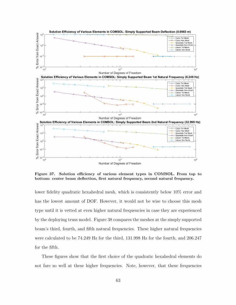
Figure 37. Solution efficiency of various element types in COMSOL. From top tobottom: center beam deflection, first natural frequency, second natural frequency.
lower fidelity quadratic hexahedral mesh, which is consistently below 10% error and
has the lowest amount of DOF. However, it would not be wise to choose this mesh
type until it is vetted at even higher natural frequencies in case they are experienced
by the deploying truss model. Figure 38 compares the meshes at the simply supported
beam’s third, fourth, and fifth natural frequencies. These higher natural frequencies
were calculated to be 74.249 Hz for the third, 131.998 Hz for the fourth, and 206.247
for the fifth.
These figures show that the first choice of the quadratic hexahedral elements do
not fare so well at these higher frequencies. Note, however, that these frequencies
63

Figure 38. Solution efficiency of various element types in COMSOL. From top tobottom: third natural frequency, fourth natural frequency, fifth natural frequency.
are quite high: 74 Hz for the third natural frequency, 131 Hz for the fourth, and
205 Hz for the fifth. Compared to the first natural frequency of 8.25 Hz, such high
frequencies may not even be sustainable for the brittle carbon fiber material that is
envisioned to be used. Additionally, the mesh types that do fare better at these high
frequencies require much more DOF. Since the test here models just one longeron,
scaling the DOF to the entire system multiplies the DOF seen here by about 36
times. (4 battens + 4 longerons for each of the 4 cells, plus the 4 base battens.)
Therefore, the quadratic hexahedral mesh was still chosen and the risk of the mesh
not performing at higher frequencies was accepted.
64

Mesh Computation Time Considerations.
At first glance it would seem that the use of higher order elements to both increase
model accuracy and decrease the system DOF is a win-win. However, there is a very
important caveat that should be mentioned: increase simulation time. Higher order
elements require more complex formulations that carry over into the system stiffness
matrix. Although the system matrix is smaller due to the reduced amount of DOF,
the matrix itself is much more dense. Figure 39 visualizes the stiffness matrices of two
different meshes applied to the simply supported beam used in the previous section.
The plot on the left shows the nonzero values in the stiffness matrix for a linear
tetrahedral mesh. The mesh has 708 DOF, and the matrix is comprised of 10,918
nonzero values, meaning that the matrix is approximately 2% filled. By comparison,
the plot on the right shows the nonzero values in the stiffness matrix for the same
geometry discretized by a quadratic hexahedral mesh. This mesh has 351 DOF, but
has 29,123 nonzero values. The matrix is approximately 24% filled. Therefore, even
though the DOF of the simulation is halved by using quadratic hexahedrons, the total
number of values that the solver must deal with is tripled. Anecdotally, the simulation
time for the four cell truss increased from approximately 2.5 hours to 4 hours when
switching from a linear tetrahedral mesh to a quadratic hexahedral mesh of similar
discretizations shown here. This poses a significant increase to the simulation time,
however it is accepted here as the accuracy gains of the quadratic mesh are more than
worth it.
3.7 Deployment Envelope
An important measure of the health of the truss deployments is the envelope in
which the deployment occurs. If the deployment is too wild and has a large envelope,
then it may intersect with other geometries on the finished aperture structure while
65

Figure 39. Left: Nonzero values of linear tetrahedral mesh stiffness matrix. Right:Nonzero values of quadratic hexahedral mesh stiffness matrix.
it deploys. Therefore a scheme was created to track the displacements of the end
fittings to quantify the deployment envelope.
In COMSOL, the displacements and rotations of two end fittings that are situated
diagonally from each other on each cell are entered into an export data table. (Diag-
onally situated here, for example, means the positive Y fitting on the positive X face,
as well as the negative Y fitting on the negative X face.) The data table contains the
displacements of the end fittings at each time step during the simulation. It is then
exported into MATLAB, where it is trimmed of any extraneous data and saved as a
binary MATLAB file (.mat). Next the file is imported into a MATLAB script (Ap-
pendix 6.1), and assuming that the batten square connecting the end fittings is rigid,
the locations of the other two corners are extrapolated via simple geometry. Finally,
the script determines the maximum and minimum displacements achieved during the
simulation for the corners of all four truss cells. The output of this script file are the
maximum and minimum displacements for each axis, from which a bounding box of
the simulation can be made.
66

3.8 Summary
Section 3.2 showed how the as-designed geometry works and how it can be simpli-
fied for simulation purposes. The simplification not only decreases the computational
overhead of the simulation significantly, but also places an emphasis on the deploy-
ment of the structure itself and not the performance of the structure’s individual
components. Section 3.3 calculated new material properties for the simplified geom-
etry which enables it to behave similarly to the as-designed components. Section 3.4
gave examples of the modeling nomenclature on the simulation model to show how
the different components are called out in this work. Section 3.5 walks through the
process of setting up the simulation in COMSOL. It exemplifies several aspects of the
setup and gives an in-depth explanation on how the cables are created. Section 3.6
lends credence to the decision of using a quadratic hexahedral mesh on the geometry
because it represented the best combination of accuracy and economy for these simu-
lations. Finally, Section 3.7 explained how the deployment envelope of the simulation
will be calculated using MATLAB.
67

IV. Analysis
4.1 Introduction
The purpose of this chapter is to show and analyze the results of the truss de-
ployment simulations. Although one of the main goals of this work was to create
a simulation of the truss in COMSOL, it was also thought that additional simula-
tions with differing parameters would be useful. Such simulations not only show how
flexible COMSOL can be when adjusting parameters, but can also help determine po-
tential susceptibilities of the structure to certain adjustments. Please refer to Chapter
3 when viewing the results, as the nomenclature established there will be used ex-
tensively in this chapter. Section 4.2 will analyze the uncontrolled deployment of the
truss structure and show the manner in which it deploys. This includes graphical view
of the structure with the surfaces displaying the von Mises stress, plots of the applied
hinge moments in the longeron-longeron hinges that motivate the deployment, plots
of the cable forces that occur when the truss cells reach their deployed state, and
plots of the von Mises stress within the longerons with an emphasis placed on their
behavior during the hinge-locking “lockout” events. Next, Section 4.3 will show two
different simulations in which the truss structure was placed into a rotating frame.
In one simulation the rotating frame is set to rotate at 5 degrees per minute, and the
other simulation is set to rotate at 60 degrees per minute. Both rotations are about
the Z-axis and are meant to show how the deployment reacts to centripetal forces
acting on the arms. The rates of rotation are built to taper as the structure deploys
and the moment of inertia increases. Section 4.4 explores what happens when one
weak hinge is introduced into the structure. In this case, a “weak hinge” is a hinge
that only applies 80% of its moment to the longeron-longeron hinge joint. Here, the
susceptibility of the deployment to manufacturing flaws is shown. In total eight simu-
68

lations were run, each with one weak hinge on the top or bottom of each cell. Finally,
Section 4.5 shows how the truss deploys in a “controlled” manner. Controlled here
meaning that the deployment order of the individual truss cells is delayed so that a
truss cell will be fully open before its adjacent neighbor is deployed. Two simula-
tions were run, one with the deployment order from root-to-end, and the other from
end-to-root, as the truss was designed.
The main model parameters chosen for all of the simulations remain the same
throughout this analysis unless otherwise specified. They are shown in Table 6 and
reflect the values that were not necessarily as-designed, but allowed the first uncon-
trolled deployment simulation to successfully deploy with a reasonable simulation
time. In a real world deployment scenario, such a large structure would not be de-
signed to deploy in under eight seconds.
Parameter ValueLongeron-Longeron Hinge Spring Constant 10 Newton-meters/radian
Longeron-Longeron Hinge Pre-Deformation Angle 3.14 radianLongeron-Longeron Hinge Damping Coefficient 1 Newton-meter-seconds/radian
Cable Spring Constant 25 Newton-metersCable Damping Coefficient 5 Newton-meter-seconds
Cable Target Tension 10 Newtons
Table 6. Static Model Parameters
4.2 Uncontrolled Deployment
The uncontrolled deployment of the four cell truss simulation was the first to
be successfully completed. It was the testbed from which all of the best settings
were found for a successful deployments, as outlined in the previous chapter. This
model is notable for having the least amount of constraints placed on it, which is
the most likely explanation for its early success. To reiterate, the base zeroth cell is
fully constrained in space and the hinge moments are applied instantaneously at the
69

beginning of the simulation. From there, the structure deploys as a function of the
hinge moments and the geometry through which the moments are transmitted.
Initial Displacement.
This subsection graphically shows the deployment of the truss system at select
time intervals. Care will be taken to highlight some of the important aspects of the
deployment during certain simulation times. Due to the limitations of the paper
media, this is the only section that will show a full play-by-play simulation of the
truss. All other section serve merely to show the differences from this particular
simulation. The time steps at which the simulation is shown are chosen to showcase
the more important movements of the deploying truss.
Figure 40. Uncontrolled deployment simulation displacement at 0 seconds.
Figure 41. Uncontrolled deployment simulation displacement at 0.5 seconds.
70

Figure 42. Uncontrolled deployment simulation displacement at 1 second.
Figure 43. Uncontrolled deployment simulation displacement at 1.5 seconds.
First Cell Lockout Event.
Figures 40 through 43 show the displacement of the truss during the first 1.5
seconds. In Figure 41, only Cell 4 is deploying even though all of the hinge moments
are applied in the structure. This shows that the “pushback” force from Cell 4 as
it expands outwards is enough keep the rest of the cells in their stowed positions.
Figures 42 and 43 show that this continues during most of Cell 4’s deployment.
Figure 44. Uncontrolled deployment simulation displacement at 2 seconds.
71

Figure 45. Uncontrolled deployment simulation displacement at 2.25 seconds.
Figure 46. Uncontrolled deployment simulation displacement at 2.4 second.
Figure 47. Uncontrolled deployment simulation displacement at 2.7 seconds.
72

Here Figure 45 shows that as Cell 4 reaches its hinge lockout angles, Cell 3 begins
to deploy. At this point in the simulation, the applied moments from Cell 4’s longerons
are closing in on zero, allowing the next truss cell to start moving. Figure 45 shows
the lockout of the top longerons in Cell 4. The top longerons lock first because they
are shorter than the bottom longerons yet have the same applied moment. The red
arrows have now appeared as well, indicating that the shaping cable forces are now
active1. Although the bottom longerons must combat these cable forces from the top
lockout event, the applied moment is still great enough for the bottom longerons to
lockout in Figure 46. Figure 47 completes Cell 4’s deployment by showing both cable
forces being activated and pulling on the truss to form the desired shape.
Figure 48. Uncontrolled deployment simulation displacement at 2.23 seconds.
The following figures show the lockout event of the top longerons in detail. The
snapshots are taken at the peak and middle amplitudes of the oscillatory motion
caused by the lockout event for one cycle. During the motion, the time steps are
greatly reduced in order to properly model the motion, and so the time steps are only
a selection for the tight cluster found in the simulation. Figure 48 highlights the local
area that will be focused on for these figures.
Although the size of the time steps vary throughout the lockout event, they average
1The top structural cables are active at this point as well, but are not shown in these simulationresults. Please note that the direction of the arrows is the same as the direction of the force beingapplied, and that the size of the arrows is based on the magnitude of the force. Therefore, a largearrow indicates a large force being applied, and a small arrow indicates a small force being applied.
73

Figure 49. Uncontrolled deployment simulation stress at 2.27 seconds. (Cropped)
Figure 50. Uncontrolled deployment simulation stress at 2.30 seconds. (Cropped)
Figure 51. Uncontrolled deployment simulation stress at 2.33 seconds. (Cropped)
Figure 52. Uncontrolled deployment simulation stress at 2.364 seconds. (Cropped)
74

approximately 5 milliseconds, or half of the 10 millisecond target time step. Figures
49 through 52 visually represent half of an “oscillatory cycle” forced as a result of
the lockout event, and in reality this motion is comprised of approximately 20 time
steps. As the longerons bend through this cycle, the von Mises stress in the longerons
increases as a function of the bending magnitude. The values of the stress are not
very important here, as they are merely representative of deploying truss. Instead, the
stress is really indicating the amount of bending in the members during the simulation
and proves that COMSOL can capture this motion after lockout.
Figure 53. Von Mises stress of Cell 4’s longeron lockout events during uncontrolleddeployment simulation (Cropped).
Figure 53 contains the plot of the von Mises stress probes attached to the domains
of the longerons2. The figure more clearly represents the oscillatory motion spoken
of in the previous paragraph. The frequency of the oscillations is important here,
as it is approximately 7 cycles per second. This is quite close to the first natural
bending frequency of 8.54 Hz that was found in Section 3.6, and indicates that the
longerons do not experience the higher frequencies in which the chosen quadratic
hexahedral mesh performed poorly. The oscillations of the longerons can also be seen
to damp out in approximately a half second. Although the only damping present in
2The blue and red lines represent the top longerons and the cyan and green lines represent thebottom longerons.
75

the structure lies in the longeron-longeron hinges, the damping effect in the stress is
most likely a result of the numerical solver used for the simulation. It should also be
noted that there are some small perturbations in the stress before the lockout event
from 2 to 2.2 seconds. Such behavior may be attributed to Cell 3, which at this time
is beginning to open as the applied moments from Cell 4 drop to zero upon lockout.
As Cell 3 opens, the base from which Cell 4 is propelled becomes less stiff, resulting
in the extraneous motion seen here.
Cell 3 Lockout Attempt and Miss.
Figure 54. Uncontrolled deployment simulation displacement at 3 seconds.
Figure 55. Uncontrolled deployment simulation displacement at 3.5 seconds.
Figures 54 through 60 show the deployment of Cell 3. This deployment is not so
successful as the bottom longerons regress in their deployment motion. The bottom
longerons are longer, and causes some vertical motion of Cell 4 which resides on the
more positive Z face of Cell 3. The vertical motion means that when the shorter top
76

Figure 56. Uncontrolled deployment simulation displacement at 3.75 seconds.
Figure 57. Uncontrolled deployment simulation displacement at 4 seconds.
Figure 58. Uncontrolled deployment simulation displacement at 4.3 seconds.
Figure 59. Uncontrolled deployment simulation displacement at 4.5 seconds.
77

Figure 60. Uncontrolled deployment simulation displacement at 4.8 seconds.
longerons lockout first, there are sharper angles in the negative Y frame-to-longeron
hinges and the positive Y longeron-to-frame hinges. As a result the distance that
the cables must stretch is larger, and the force exerted by the cables overpowers the
applied hinge moment of the bottom longerons.
Figure 61. Cable forces of Cell 3 during uncontrolled deployment simulation (Cropped).
Figure 61 shows the applied cable forces in Cell 3 and Figure 62 shows the applied
moment in Cell 3’s longerons. The blue and red lines on both graphs represent the
negative Y to positive Y shaping cables in the cell and the top longeron hinges. At
approximately 4 seconds, the applied hinge moments of the top longerons reaches
zero where the lockout angle of the longerons reside. At this point in time, there is
a spike in the cable forces for the aforementioned shaping cables that form a truss
triangle. Here the applied spring moment of the lower longerons, shown in cyan and
78

Figure 62. Applied hinge moment of Cell 3’s longerons during uncontrolled deploymentsimulation (Cropped).
green in Figure 62, is only 10 Newton-meters. For the geometry of the truss cell at
this point, it is not enough to overcome the applied cable forces of approximately 37
Newtons. Thus, the lower longerons are forced to reverse their direction and build
more moment after this event. Later in the simulation, however, the geometry is such
that the applied hinge moment of 18 Newton-meters combats the 50 Newtons of cable
forces and is able to lockout at approximately 7.7 seconds. Although there appears to
be a simple relation between the cable force and applied moment here that dictates
a successful lockout, it is in fact more complicated. As the following Figures show,
the entire kinetic motion of the structure during deployment is a major factor in cell
deployment success.
Simulation Energies.
Figures 63 through 71 show the full deployments of Cells 1, 2, and 3. All of these
deployments were in some way aided by the momentum of the structure moving
outwards which “pulled” the cells open. This energy that is used to successfully
deploy these Cells is critical to the deployment success of the truss arm. The next
figures of this section show the raw data of the simulation, where the cable forces
79

Figure 63. Uncontrolled deployment simulation displacement at 5.25 seconds.
Figure 64. Uncontrolled deployment simulation displacement at 5.6 seconds.
Figure 65. Uncontrolled deployment simulation displacement at 6 seconds.
Figure 66. Uncontrolled deployment simulation displacement at 6.4 seconds.
80

Figure 67. Uncontrolled deployment simulation displacement at 6.6 seconds.
Figure 68. Uncontrolled deployment simulation displacement at 6.8 seconds.
Figure 69. Uncontrolled deployment simulation displacement at 7 seconds.
Figure 70. Uncontrolled deployment simulation displacement at 7.4 seconds.
81

Figure 71. Uncontrolled deployment simulation displacement at 7.7 seconds.
applied to the Cells can be directly compared to the applied hinge moment. In these
figures it is possible to see that for the cells closer to the base, the cable to hinge
moment relationships are far greater than that of Cell 3’s lower longerons which
failed to properly deploy. To further support this claim, Figure 72 shows the total
kinetic, strain, and summed energies of the entire structure. Keep in mind that the
kinetic strain energy is calculated from the mesh of the domains in the structure, but
that strain energy also includes the cables and hinges. The summed energy is merely
an addition of the kinetic and strain energies.
Figure 72. Uncontrolled deployment simulation kinetic and strain energies.
At the beginning of the simulation, the strain energy is at its highest and the ki-
netic energy is at its lowest, as one would guess. As each truss deploys, however, the
kinetic energy keeps building even though the longerons lockout at certain times be-
82

cause the cells farther out are pushed by the cells nearer the base. Interestingly, both
energies show the same disruptions caused by the lockout events. At approximately
6.4 seconds, the kinetic energy suddenly drops off as the base Cell 1 fully deploys
and stops the truss from moving outwards. Conversely, the strain energy spikes quite
suddenly, as all of the cables strain to hold and create their Cell’s intended shape.
Once Cell 3 finally locks around 8 seconds, the kinetic and strain energies form a
loose inverse relationship as the deployed truss structure moves vertically in a peri-
odic fashion. Last but not least, the summed energies of the deployment, shown in
red, and helps to explain how the structure dissipates its energy. The kinetic energy
of the truss members is mainly absorbed by themselves during the lockout events
and damped by the numerical solver. Again, the summed energies slowly decline at
first, but decay very rapidly after Cell 1 fully deploys. The notable exception being
the sharp spike in strain energy caused by the cables of Cell 3 fighting the lower
longerons finally deploying. By the end of the simulation, it is clear that the total
energy is beginning to reach its equilibrium point where only the strain energies of
the cables and truss elements are active. On its way to equilibrium, however, the sum
of the energies increases briefly from 11 to 15.5 seconds, and should not be physically
possible. Although the exact cause for the increase is not certain, it is thought that
strain energies are not being taken into account correctly.
Post Deployment Transient Motion.
Figures 73 through 88 show the remaining 12 of the total 20 seconds of the simu-
lation. Note that the structure does not uniformly move vertically and moves in more
of a “wave” fashion. Such motion can be attributed not only to the unequal length
longerons throughout the truss structure, but also the differing times of deployments.
Most of the motion seen throughout this time period is a result of the shaping cables
83

Figure 73. Uncontrolled deployment simulation displacement at 8 seconds.
Figure 74. Uncontrolled deployment simulation displacement at 8.5 seconds.
Figure 75. Uncontrolled deployment simulation displacement at 9 seconds.
Figure 76. Uncontrolled deployment simulation displacement at 9.5 seconds.
84

Figure 77. Uncontrolled deployment simulation displacement at 10 seconds.
Figure 78. Uncontrolled deployment simulation displacement at 10.5 seconds.
Figure 79. Uncontrolled deployment simulation displacement at 11 seconds.
Figure 80. Uncontrolled deployment simulation displacement at 12 seconds.
85

Figure 81. Uncontrolled deployment simulation displacement at 13 seconds.
Figure 82. Uncontrolled deployment simulation displacement at 14 seconds.
Figure 83. Uncontrolled deployment simulation displacement at 15 seconds.
Figure 84. Uncontrolled deployment simulation displacement at 16 seconds.
86

Figure 85. Uncontrolled deployment simulation displacement at 17 seconds.
Figure 86. Uncontrolled deployment simulation displacement at 18 seconds.
Figure 87. Uncontrolled deployment simulation displacement at 19 seconds.
Figure 88. Uncontrolled deployment simulation displacement at 20 seconds.
87

trying to form the final parabolic shape of the reflector. Remember that the size of
the arrows indicate the force being applied. The serialized cells moving with each
other, fighting to find their own equilibrium often upsets that of its neighboring cell.
Simulation Data.
Figure 89. Uncontrolled deployment simulation cables forces of Cell 1.
Figure 90. Uncontrolled deployment simulation applied hinge moments of Cell 1.
Figures 89 through 96 show the relationships between the cable forces and hinge
moments for each cell. It is interesting to note here that although the top longerons
are shorter and deploy first in Cells 3 and 4, it is the bottom longerons that deploy
88

Figure 91. Uncontrolled deployment simulation cables forces of Cell 2.
Figure 92. Uncontrolled deployment simulation applied hinge moments of Cell 2.
Figure 93. Uncontrolled deployment simulation cables forces of Cell 3.
89

Figure 94. Uncontrolled deployment simulation applied hinge moments of Cell 3.
Figure 95. Uncontrolled deployment simulation cables forces of Cell 4.
Figure 96. Uncontrolled deployment simulation applied hinge moments of Cell 4.
90

first in Cells 1 and 2. This phenomena is most likely a result of the geometry con-
figuration at the later stages of the deployment. Figures 97 through 100 show the
longeron stresses of each Cell during deployment. The first thing to notice on the
stress plots is the initial stress of each cell at the start of the simulation. This repre-
sents the bending of the beams as the hinge moments from the hinges are applied to
the folded longerons to begin the deployment. More importantly, however, the figures
show that the stress waves from one cell’s lockout event can be seen throughout the
other cell’s. For example, Cell 4 is the first Cell to fully deploy at approximately
2.5 seconds. The deployments of Cell 4’s longerons are timed very closely together.
After this deployment, a small positive variation in Cell 3’s stress is seen at approx-
imately 2.75 seconds as the lockout event stress travels to Cell 3. Some time later
at approximately 4.5 seconds, Cell 2 experiences a similar positive stress variation.
Although not conclusive, the results suggest that Cell 4’s lockout event stress wave
and Cell 3’s top longeron lockout event stress wave cause Cell 2’s small positive vari-
ation. Through the rest of time of the simulation similar stress wave sharing can be
seen, especially between adjacent cells. It should be kept in mind though that some
of the stresses seen in the latter parts of the simulation may also be from the slight
bending of the cells by the shaping cables. It should also be said that the magnitude
of these stresses really just indicate some displacement by the bending longerons. The
main point, however, is that these simulations show that COMSOL does translate the
events from each member in the system through the declared hinges (which are not
meshed with flexible elements) to other members in a significant fashion.
The deployment envelope is one of the most important analyses done to these
simulations. Table 7 shows the results from the MATLAB code written to determine
the maximum displacements achieved by the truss in 3D space. Keep in mind that the
truss itself is centered upon the origin of the XY Plane. Therefore, the upper and lower
91

Figure 97. Uncontrolled deployment simulation longeron stress of Cell 1.
Figure 98. Uncontrolled deployment simulation longeron stress of Cell 2.
Figure 99. Uncontrolled deployment simulation longeron stress of Cell 3.
92

Figure 100. Uncontrolled deployment simulation longeron stress of Cell 4.
bounds for X-axis merely denote the width of the truss with some added horizontal
displacement of approximately 4-5 centimeters3. It is interesting that the trusses’
deployment shows any horizontal movement at all since the applied forces almost
exclusively reside in the YZ-Plane. However, the horizontal forces of the structural
cables may cause this motion as they will not always be perfectly symmetric due
to a relatively high 1% tolerance factor imposed on the dependent variables of the
simulation. The lower bound of the Y-displacement is almost a meter lower than the
height of the cells (5.31 meters) centered at the origin. The upper bound of Y, shows
an even more significant peak of almost 10 meters. Both of these may be of some
concern in future work when the rest of the reflector aperture is constructed around
this deployment. The upper Z bound validates that the solid modeling of the truss
done in the early stages of this work was done correctly. The as-designed diameter
of the complete sparse aperture is supposed to be approximately 150 meters, and
one half of one truss arm extends roughly one quarter of this diameter. Lastly, the
negative Z bound is zero, as one would expect with the model fully constrained on
the XY Plane.
3The nominal width of the truss cells is 8.74 meters and the nominal height of the truss cells is5.31 meters.
93

Completed Deployment X Y ZUpper Bound (m) 4.4710 6.0679 37.9799Lower Bound (m) -4.4710 -2.6422 0
Uncontrolled Deployment X Y ZUpper Bound (m) 4.4430 9.7763 37.8630Lower Bound (m) -4.5435 -3.6698 0
Table 7. Uncontrolled Deployment Simulation Deployment Envelope
4.3 Uncontrolled Deployments with Centripetal Acceleration
The practice of exploiting centripetal acceleration of orbiting bodies is nothing
new. It was thought that by adding a rotating frame to the simulation that perhaps
a better deployment behavior could be achieved. In this instance, two simulations
were run: one with an initial rotation of 5 degrees per minute, and another with an
initial rotation of 60 degrees per minute. Please note that a angular velocity of 60
degrees per minute is very excessive for a structure of this size in space, and is only
used here to exemplify COMSOL’s capabilities. Both of these rotations speeds are
initial, since the deployment of the truss arm creates a larger moment of inertia to
slow the rotation down. Both simulations place a rotating frame about the Z-axis, the
center of which would be the hub of the four arms for the complete sparse aperture.
A simple function was created in COMSOL to control the angular velocity of the
rotating frame as a function of the varying moment of inertia of the truss arm. An
initial angular momentum was assumed for the stowed truss that was calculated as
a simple centroid mass. The initial angular momentum is them divided by the same
mass multiplied by the square of the increasing radius. The radius is determined by
the Z displacement of Cell 2’s frame connectors. This is the simplest formulation
for moment of inertia and is used only to get some form of diminishing rotation in
the simulation. All of these terms are used to solve for an angular velocity, which is
applied to the rotating frame physics node built into the simulation model. Figure 101
94

shows this created function against the time steps of the simulation, and Equation 15
shows the basic kinetics used to determine the angular velocity of the rotating frame.
Figure 101. Uncontrolled deployment simulations in rotating frames.
H = mr2ω → ω =Hinitial
mr2centroid(15)
Where H (Angular Momentum), m (Mass), rcentroid (Mass Centroid Radius), and
ω (Angular Velocity).
This figure illustrates how quickly the moment of inertia changes for the truss.
At approximately 4 seconds, the rotating frame has all but stopped acting on the
structure. One would hope that the rotation would halt closer to the truss’s fully
deployed state, however that is not the case using this methodology. This method-
ology being used may have been grossly oversimplified, however the results gleaned
from these simulations are still valuable and show how the model reacts to the ap-
plied centripetal acceleration, albeit only for the cells that are the first to deploy.
The following subsections show how the deployment speeds of the simulations differ
from the first uncontrolled simulation already detailed and will then show how the
deployment speeds affected the lockout stress events. Both subsections will focus on
Cells 3 and 4, as they were most affected by the centripetal acceleration.
95

Cell Deployment Speed.
As the frame rotates with the deploying truss in it, it would be reasonable to expect
that the added centripetal force would pull the trusses out from their stowed position
faster than if it had not been there. Upon analysis of the simulations, however, this
is not really the case. Figure 102 shows only two distinct lines even though there
are six sets a data present: the applied hinge moment for one of the top longerons of
Cells 3 and 4 for the uncontrolled deployment, the deployment with an intial 5 degree
per minute of rotation, and the deployment with an initial 60 degrees per minute
of rotation. The presence of only two distinct lines means there was no difference
between any of these simulations. This is most likely a result of the low density
of the truss members, which are not affected too much by the applied centripetal
acceleration. It should also be restated that the hinges contain a small amount of
damping, which would keep the longerons from accelerating too quickly.
Figure 102. Select top longeron applied hinge moments in uncontrolled deploymentsimulations in rotating frames.
However, upon zooming into the graphs at the lockout event locations, some
disparities in the data appear. Figure 103 is a cropped image of Figure 102 and shows
the overshoot exhibited by the hinges in the rotating frame simulations. Although
minimal, this kind of behavior at least validates that the rotating frame was indeed
applied to the structure. If one were to look to Cell 3’s results in this manner, the
96

results are the same, albeit not as pronounced. These plots mean that although
the hinges did not lock any faster, they did lock harder which means that more
displacement in the locked longerons can be expected.
Figure 103. Select top longeron applied hinge moments in uncontrolled deploymentsimulations in rotating frames. (Cropped)
Cell Lockout Stress.
Increased displacement in the longeron-longeron hinges during the lockout event
means increased displacement and stress in the members. Indeed, Figure 104 shows
that the added centripetal acceleration from the rotating frame increases the stress
sustained by the longerons during lockout. The highest stress is seen in the longerons
from the faster rotating frame simulation. Not only is this stress higher, but even
after the lockout event, the longerons exhibit some harmonic motion that was not
present in the original non-rotating simulation. It seems as though the added force
of the rotating frame is adding some kind of axial load to the extended longerons
and is causing this extra motion. Although it should be said that such motion may
be more indicative of the simplified geometry or the numerical solver tolerances, the
fact remains that rotating the structure during deployment may result in some added
97

motions.
Figure 104. Cell 4 top longeron von Mises stress in different rotating frames. (Cropped)
Cell 3 exhibits the same harmonic disturbances as Cell 4, as seen in Figure 105,
but the peak stress of the faster rotating frame simulation is more interesting. It
appears as though the additional force applied to the completely deployed Cell 4
has pulled on Cell 3. This has created a much large peak stress than the other
two simulations. This higher peak stress is even accompanied by a higher frequency
response, which is generally not desirable in a structure such as this. Therefore, these
results suggest that rotating the structure during the deployment does not seem to
positively influence it at all.
Figure 105. Cell 3 top longeron von Mises stress in different rotating frames. (Cropped)
From a larger perspective, the last two truss Cells 1 and 2 do not exhibit such
98

notable increases seen in Cells 3 and 4. Most likely the damped hinges contained
within Cells 1 and 2 were able to control the deployment so that the momentum from
the first two deployments did not damage the structure. It should also be mentioned
that the same Cell 3 bottom longeron initial miss occured as well, and that the
remainder of the simulations emulated the non-rotating frame of the first. More
importantly, comparison of the stress results in both cells reveals how the numerical
solver may be sensitive enough to model the entirety of the stress behaviors in the
longerons. Take Figure 105 for example. From 7.5 to 8 seconds, all three plots overlay
onto each other. From 5.5 to 6 seconds, only the slower rotating frame exhibits any
harmonic motion. These differences in results can most likely be directly attributed
to the 10% tolerance factor imposed on the time steps in the solver settings. This
setting allows the simulation to be run in a in a few hours on relatively low power
computers and captures the global motion of the simulations quite well. Table 8
shows the deployment envelopes of these simulations.
Completed Deployment X Y ZUpper Bound (m) 4.4710 6.0679 37.9799Lower Bound (m) -4.4710 -2.6422 0
Uncontrolled Deployment X Y ZUpper Bound (m) 4.4430 9.7763 37.8630Lower Bound (m) -4.5435 -3.6698 0
5 Degrees per Minute Initial Rotation X Y ZUpper Bound (m) 4.4283 9.8037 37.8550Lower Bound (m) -4.5370 -3.6490 0
60 Degrees per Minute Initial Rotation X Y ZUpper Bound (m) 4.4850 9.9063 37.8430Lower Bound (m) -4.4801 -3.6472 0
Table 8. Various Deployment Simulation Deployment Envelope
99

4.4 Weakened Hinges
Manufacturing defects are a fact of life when it comes to fabricating engineering
designs. The space industry spends a great deal of money on flight-ready hardware to
reduce the chances of any individual part failing. As has happened many times in the
past, however, if something can fail, it will fail. Therefore the purpose of this section
is to explore the deploying truss structures susceptibility to manufacturing defects. In
total, eight simulations were run. Each simulation places a “weak hinge” in the top or
bottom of each cell. Here, “weak” means a longeron-longeron hinge that only applies
80% of its intended torque4. It was thought that since these hinges are what motivates
the structure to deploy, that if one were to be outside manufacturing specifications,
that they may compromise the deployment of the structure. From anecdotal evidence
gleaned from creating these simulations, if one of these hinges applies no moment
whatsoever, then that cell will fail to deploy all together. All other hinges in the
structure are much simpler than these longeron-longeron hinges, and will reach steady
state via the shaping cables that dictate the truss arm’s final shape. Instead of
showing the results from each individual simulation, this section will only discuss
how the simulation with the particular defect differed from the nominal deployment
shown in Section 4.2. Concluding this section will be some general remarks on the
observed behavior of the structure in response to these manufacturing defects. A
table of the deployment envelopes for each simulation will also be included at the
end.
Weak Hinge in an Upper Longeron of Cell 1.
With a weak hinge present on the negative X positive Y longeron of the base Cell
1, the truss was able to fully deploy. However, the structure had some trouble coping
480% was chosen somewhat arbitrarily and represents a value at which a single truss simulationwould just barely achieve its lockout state in multiple observed attempts.
100

with the hinge moment deficit. Figure IV.106(a) shows the weak hinge in place in
Cell 1. Figures IV.106(a) through IV.106(d) show that the bottom longerons of Cells
2-4 failed to deploy on their first attempt. Meanwhile, all of the top longerons in the
entire structure were able to deploy quite easily. It is also interesting that the bottom
longerons of Cell 4 were the last to deploy in the simulation. The exact cause for this
behavior is not very well known, and may only reveal itself through further analysis
of the following simulations. Although not included in this work, the stresses and
cable forces of the deploying structure remain largely the same for this deployment
simulation.
Weak Hinge in a Lower Longeron of Cell 1.
The weak c1.nxny.lglg hinge impeded the structure from fully deploying in this
scenario. Again, it is only the lower longerons that have issues when a weak hinge
is introduced in Cell 1. It is slightly counter-intuitive to think that a weaker lower
hinge in Cell 1 would keep Cell 4’s lower hinges to deploy. The weak hinge should
allow for less push back on Cell 4’s lower longerons, enabling them to deploy easier.
However, the weak hinge may be affecting the geometry throughout the simulation
and may be less conducive to a lower longeron lockout event. Indeed, Table 95 shows
that the deployment envelopes for both Cell 1 weak hinge deployments causes more
vertical, positive Y motion than the original uncontrolled deployment. Figure 108
shows the truss at the end of the simulation. Note that these weak hinge simulations
were run up to 25 seconds to capture more of the post-deployment, transient motions
of the structure. The stress and cable forces were once again on par with that of the
uncontrolled simulation, and did not show any significant increase.
5This table is shown in the final subsection of this section.
101

(a) Cell 1 applied hinge moment. (Cropped) (b) Cell 2 applied hinge moment. (Cropped)
(c) Cell 3 applied hinge moment. (Cropped) (d) Cell 4 applied hinge moment. (Cropped)
Figure 106. Applied hinge moments of uncontrolled deployment with hinge c1.nxpy.lglgset to 80%.
102

(a) Cell 1 applied hinge moment. (Cropped) (b) Cell 2 applied hinge moment. (Cropped)
(c) Cell 3 applied hinge moment. (Cropped)
(d) Cell 4 applied hinge moment.
Figure 107. Applied hinge moments of uncontrolled deployment with hinge c1.nxny.lglgset to 80%.
103

Figure 108. Incomplete truss deployment at final simulation time with weak lowerlongeron-longeron hinge in Cell 1 (c1.nxny.lglg).
Weak Hinge in an Upper Longeron of Cell 2.
The weak top hinge (c2.nxpy.lglg) kept the truss structure from fully deploying.
Figure 109(a) shows the hinge moments for Cell 1, which progress similarly to the
original uncontrolled deployment simulation. Figure 109(b) shows that Cell 2 does
not have a failed attempt at deploying, but rather is delayed thanks to the weaker
hinge. Although one weak hinge makes the cells asymmetric in their initial behavior,
they eventually converge back to symmetry as the cell finalizes its deployment. Cell 3
again has some trouble deploying, but is not as bad as Cell 4, which failed to deploy
throughout the simulation. It looks as though Cell 4 will not ever fully extend in this
deployment mode as applied hinge moments are trending towards a horizontal line.
Perhaps Cell 4 would eventually lockout if the structure was given enough time to
stop moving altogether. Again, the likely culprit in this incomplete deployment is the
more vertical motion caused by the weak hinge, as shown in Table 9. The stress and
cable forces showed no significant changes that would affect the deployment.
Weak Hinge in a Lower Longeron of Cell 2.
Creating a weak hinge in c2.nxny.lglg affected the deployment of the truss arm
quite dramatically. Figure 111 illustrates how poorly this deployment went. First
off, the top longerons never fully extended. The shape of the geometry around 7
104

(a) Cell 1 applied hinge moment. (Cropped) (b) Cell 2 applied hinge moment. (Cropped)
(c) Cell 3 applied hinge moment. (Cropped)
(d) Cell 4 applied hinge moment.
Figure 109. Applied hinge moments of uncontrolled deployment with hinge c2.nxpy.lglgset to 80%.
105

Figure 110. Incomplete truss deployment at final simulation time with weakc2.nxpy.lglg hinge.
seconds caused a large spike in the shaping cable forces (Figure 112) that oppose
the top longerons in Cell 1 (Figure 113). This spike in addition to the upward mo-
mentum of the deploying truss causes the entire structure to swing upwards. The
upward momentum was most likely caused by the incomplete deployment of all of
the cells occuring almost simultaneously approximately one second before Cell 1’s
top longerons deployment failure. It is also interesting to note that the weak bottom
hinge on the negative X face of the trusses translates to Cell 4, whose “nxny” never
deployed throughout the simulation. This phenomena is quite strange as Figure 114
shows that this hinge did indeed reach its lockout rotation. Perhaps the default lock-
ing hinge settings within COMSOL were not strict enough to keep the hinge closed,
or the solver tolerances were not close enough to catch the lockout. Once again, the
stresses experienced by the structure were within normal ranges. Table 9 shows just
how much vertical travel the truss underwent during this simulation.
Weak Hinge in an Upper Longeron of Cell 3.
In contrast to the previous two simulations, creating a weak hinge in the top of Cell
3 had very little effect on the deployment. Figures 115(a) through 115(d) show that
there was little change in the deployment of the truss compared to the uncontrolled
dpeloyment. Notably, the bottom longerons of Cell 4 were once again delayed in its
106

Figure 111. Incomplete truss deployment at final simulation time with weakc2.nxny.lglg hinge.
Figure 112. Cable forces of Cell 1 in c2.nxny.lglg weak hinge simulation.
Figure 113. Applied hinge moments of Cell 1 in c2.nxny.lglg weak hinge simulation.
107

Figure 114. Applied hinge moments of Cell 4 in c2.nxny.lglg weak hinge simulation.
deployment, but were able to lockout around 9 seconds into the simulation. Figure
115(c) shows that the stronger of the two hinges will cause the weaker hinge lockout
at the same time as the stronger. There is some delay in Figure 115(b) for Cell 2 to
deploy, however it eventually does. The most interesting aspect of this simulation is
that the weaker hinge in Cell 3 allows it to deploy on its first attempt, which does
not happen with the stock settings in the uncontrolled deployment. This comes at a
cost of Cell 4 being delayed to deploy, but may lead to some thoughts on varying the
spring stiffnesses throughout the truss to create smoother deployments in the future.
There were not any notable changes in the stresses or cable forces of this simulation.
Weak Hinge in a Lower Longeron of Cell 3.
The weak c3.nxny.lglg hinge did not have a great effect on the truss deployment. If
anything, the weaker hinge pronounced Cell 3’s problems with its lower longerons seen
in the uncontrolled deployment, as seen in Figure 116(c). Other than this, there was
nothing remarkable about this simulation. The stresses, cable forces, and deployment
envelope showed no signs of any significant behavior.
Weak Hinge in an Upper Longeron of Cell 4.
A weaker hinge in an upper longeron of Cell 4 does not affect the deployment of
the structure significantly. The lower longerons of Cells 2 and 3 were both delayed
108

(a) Cell 1 applied hinge moment. (Cropped) (b) Cell 2 applied hinge moment. (Cropped)
(c) Cell 3 applied hinge moment. (Cropped) (d) Cell 4 applied hinge moment. (Cropped)
Figure 115. Applied hinge moments of uncontrolled deployment with hinge c3.nxpy.lglgset to 80%.
109

(a) Cell 1 applied hinge moment. (Cropped) (b) Cell 2 applied hinge moment. (Cropped)
(c) Cell 3 applied hinge moment. (Cropped) (d) Cell 4 applied hinge moment. (Cropped)
Figure 116. Applied hinge moments of uncontrolled deployment with hinge c3.nxny.lglgset to 80%.
110

in their deployment. Although Cell 3 is usually always delayed, as seen in the first
uncontrolled deployment, Cell 2 is delayed by the geometry created by Cell 4. In Cell
4, the top longerons take approximately 5.5 seconds to fully extend due to the weaker
hinge. It appears as though the stronger hinge takes some time to match the rotation
of the weaker in order to fully deploy. Cell 1, as usual, is unaffected by a change so
far away from itself. The stress and cable forces show very little difference compared
to the uncontrolled simulation and the deployment envelope is unremarkable.
(a) Cell 1 applied hinge moment. (Cropped) (b) Cell 2 applied hinge moment. (Cropped)
(c) Cell 3 applied hinge moment. (Cropped) (d) Cell 4 applied hinge moment. (Cropped)
Figure 117. Applied hinge moments of uncontrolled deployment with hinge c4.nxpy.lglgset to 80%.
111

Weak Hinge in a Lower Longeron of Cell 4.
Once again a weak hinge in a lower longeron causes the truss arm to fail to deploy.
Unlike the previous examples, however, the bottom longerons of Cell 4 fail to deploy
thanks to the weaker hinge in one of the longerons. Other than this failure, the rest of
the truss structure behaves as expected. Cells 1 and 2 deploy without any hesitation,
and Cell 3 fails its first attempt. It appears as though the added mass of Cell 4 itself
on the end of the truss arm does very little to affect the rest of the truss’s deployment.
The stresses and cable forces were once again wholly unremarkable.
Observations and Remarks.
Figure 120 shows a side view of the truss arm in its deployed state for each of the
weak hinge deployment simulations. The weak hinges are shown as dashed lines, and
the deployment time for each longeron pair is represented through the thickness of the
line. The longer the time to deploy, the thicker the line. For example, if the longeron-
longeron hinge regresses, then the time it takes to recover and fully extend is four
seconds, then the line thickness is scaled by four times. If a longeron is not present
in the Figure, then the longeron failed to deploy within the simulation time. For
further clarification, the failed deployments are in red and the successful deployments
are shown in blue. Table 9 complements Figure 120 and displays the deployment
envelopes for all of the simulations discussed in this section.
The results are far from conclusive, but it might be said that the successful de-
ployment of the truss is more dependent on the lower longerons. The lower longerons
do not deploy as well as the upper longerons because they are longer yet have the
same spring-hinge moment applied to them. This decreases the lower longerons’ rela-
tive mechanical advantage and increases their deployment time. The increased lower
longeron deployment time is further reduced by the shaping cables which activate
112

(a) Cell 1 applied hinge moment. (Cropped) (b) Cell 2 applied hinge moment. (Cropped)
(c) Cell 3 applied hinge moment. (Cropped)
(d) Cell 4 applied hinge moment.
Figure 118. Applied hinge moments of uncontrolled deployment with hinge c4.nxny.lglgset to 80%.
113

Figure 119. Incomplete truss deployment at final simulation time with weakc4.nxny.lglg hinge.
once the upper longerons deploy. They also create a vertically-moving geometry that
impedes their own deployment as they move. Overall, the lower longerons may require
an adjustment in parameters to increase their chance of successful lockout.
Weak hinges in Cell 2 proved to be fatal for the deployment of the truss arm,
especially when a lower longeron contained the weak hinge. Most times, the failed
deployment was caused by the lower longerons of Cell 4. Cell 4 does not have any
added momentum from other cells connected to its positive Z face to pull it open.
Additionally, the residual swaying of the truss arms triggers the shaping cables in
Cell 4 and further impedes its lower longerons from locking out.
Many more conjectures can be made from this Section, but the main takeaway
should be that COMSOL successfully solved all of these asymmetric simulations. It
should be mentioned that setting up the different scenarios is very easy, requiring only
the weak hinge’s moment to be multiplied by 80%. Furthermore, the solver does not
need to be adjusted in these instances. The only caveat, as mentioned in Section 4.3,
is that the simulations here only represent the larger global motion of the deploying
truss. This is not a problem for the work here, which seeks to merely model the
truss’s deployment, but deeper analysis into the truss’s sensitivity to perturbations
would require a more strict time stepping protocol.
114

Figure 120. Weakened hinges study summary.
115

Completed Deployment X Y Z Uncontrolled Deployment X Y ZUpper Bound (m) 4.4710 6.0679 37.9799 Upper Bound (m) 4.4430 9.7763 37.8630Lower Bound (m) -4.4710 -2.6422 0 Lower Bound (m) -4.5435 -3.6698 0
Weak c1.nxpy.lglg Hinge X Y Z Weak c1.nxny.lglg Hinge X Y ZUpper Bound (m) 4.4221 11.4660 37.8360 Upper Bound (m) 4.4088 11.5768 37.3200Lower Bound (m) -4.5671 -2.8143 0 Lower Bound (m) -4.5898 -2.8442 0
Weak c2.nxpy.lglg Hinge X Y Z Weak c2.nxny.lglg Hinge X Y ZUpper Bound (m) 4.4157 10.0887 37.3610 Upper Bound (m) 4.4850 32.5646 36.5340Lower Bound (m) -4.5447 -2.7412 0 Lower Bound (m) -4.5216 -3.3617 0
Weak c3.nxpy.lglg Hinge X Y Z Weak c3.nxny.lglg Hinge X Y ZUpper Bound (m) 4.4225 9.4141 37.7630 Upper Bound (m) 4.553 11.6904 37.8410Lower Bound (m) -4.5197 -3.6866 0 Lower Bound (m) -4.5239 -4.5239 0
Weak c4.nxpy.lglg Hinge X Y Z Weak c4.nxny.lglg Hinge X Y ZUpper Bound (m) 4.4554 8.9432 37.7080 Upper Bound (m) 4.4306 11.1625 37.3080Lower Bound (m) -4.4677 -2.8025 0 Lower Bound (m) -4.5682 -2.7809 0
Table 9. Uncontrolled and weak hinge deployment simulation deployment envelopes
4.5 Controlled Deployments
Controlled deployments, in this context, describes a deployment in which the mo-
tivating longeron-longeron spring hinges apply their moment only when the previous
cell is fully deployed. Therefore, instead of the entire truss arm attempting to move
radially all at once, each cell takes its turn to deploy. It is thought that by timing the
release of each cell, the displacements sustained by the structural members and the de-
ployment envelope would both be reduced. Two different models were created to test
the controlled deployments. One model was set to deploy Cell 4 first, then move to
Cells 3, 2 and then 1. This is how the as-designed truss is supposed to open. Another
model was set to deploy Cell 1 first at the root of the arm, then deploy Cells 2, 3, and
then 4. Modeling these controlled deployments turned out to be more difficult than
first anticipated. Initially, it was thought to merely turn on the spring-hinges from an
“off” position at different times throughout the model. Unfortunately, early attempts
showed that completely disabling the spring-hinges near the base of the truss arm
caused some unintended consequences. In the case of the end-to-root deployment,
the bumper blocks between the batten squares would contact each other quite a lot.
This caused the solver to seek very small time steps for extended periods of time to
solve for the forces applied to the blocks. Additionally, the constant back and forth
116

motion sustained by the longerons meant that they would begin to rotate in differ-
ent directions due to the way in which the geometry was modeled. Figure IV.121(a)
shows how the longerons would begin to rotate, and Figure IV.121(b) shows how the
geometry shifts when the longerons move in this manner. Attempts to constrain the
motions of the “frlg” and “lgfr” hinges did not alleviate this behavior. When the
simulation was allowed to keep running with this awkward longeron placement, the
deployment would fail rather spectacularly (Figures IV.122(a) and IV.122(b)).
(a) Cell 1 longerons rotating at their connectionsto the batten frames.
(b) Close up of Cell 0 and Cell 1 bumper blocksmisaligning.
Figure 121. Examples of unwanted motion when longeron-longeron hinges are disabled.
To rectify this behavior, the hinges spring constants are halved, and then allowed
their full spring stiffness when it is their turn to deploy. The deployment of each
individual cell is triggered by a time delay function, which also integrates a smoothing
function to apply the moment gradually. Figure 123 show how the hinge moments
are applied throughout the simulation. For the end-to-root deployment at time zero,
the “Initial Hinge Moment Curve” is applied to all of the Cells. Also at this time,
117

(a) Cell 1 longerons rotating at awkward angles. (b) Deployment status near the end of the sim-ulation.
Figure 122. Unwanted motion propagating through simulation.
118

Cell 4’s moment curve is applied. Then throughout the simulation at different times,
the extra 50% of the spring stiffness constant is added to each cell. At four seconds,
Cell 3’s moment curve is added to the initial 50% from the beginning. For Cells 2 and
then 1, this addition occurs at 8.5 seconds and 15 seconds respectively. Conversely,
the root-to-end deployment applies the additional curves in the opposite order. It
is important to note that these simulations have a higher base spring constants for
the longeron-longeron hinges. It was found that when the original spring constant
of 10 Newton-meters/radian was used with this scheme, that half was not sufficient
to keep the longerons from rotating about their frame connection points. Also note
the smoothing applied to the moment curves. The smoothing was built-in to prevent
any shock loading on the structure during its deployment, which may have resulted
in undesirable behavior. Everything else in these simulations is setup identically to
the preceding simulations. The following subsections will describe the deployment
characteristics of each controlled simulation, and will then compare the results to the
uncontrolled simulation presented first in this chapter.
End-to-Root.
Figure 124 shows Cell 1 before it deploys, and Figure 125 shows Cell 1 directly after
both upper and lower longerons complete their lockouts. It is early in this deployment,
but so far the truss looks almost to identical to the uncontrolled deployment 46. The
sameness even extends to Cell 3, which is beginning to deploy at this point. It seems
as though the halved hinge moments are enough to move Cell 3 outwards.
Figure 126 shows Cell 3 as it is about to lockout. Notice here that some red arrows
are visible already in Cell 3, and indicates that Cell 3 will have the same deployment
issues as in the uncontrolled simulation. Figure 127 all but confirms this indication.
The uneven upper and lower longerons again create a geometry that moves vertically
119

Figure 123. Applied hinge moment curves for controlled deployment simulations.
Figure 124. End-to-root controlled deployment simulation at T = 1.9 seconds.
120

Figure 125. End-to-root controlled deployment simulation at T = 2.3 seconds.
as well as radially. This motion not only creates a larger deployment envelope, but
impedes some of the cells in their lockout motions. Again the halved spring moments
in the other cells proves sufficient to motivate the entire structure radially, albeit at
a slower pace than in the uncontrolled simulation.
Figure 126. End-to-root controlled deployment simulation at T = 3.8 seconds.
Figure 127. End-to-root controlled deployment simulation at T = 4.5 seconds.
Figure 128 shows the point in time in the simulation where Cell 2 is about to lock
its upper longerons. Notice that the lower longerons in Cell 2 are also having trouble
121

deploying completely, and Cell 1 is beginning to move as well. Figure 129 shows how
the deployment of Cell 1 exacerbates the deployment of the lower longerons of Cells
2 and 3 in that they do not have enough moment to overcome the radial motion of
the entire structure. It should also be noted here that the deployment is moving
vertically in a significant fashion.
Figure 128. End-to-root controlled deployment simulation at T = 5.6 seconds.
Figure 129. End-to-root controlled deployment simulation at T = 6 seconds.
Figure 130 shows how the lower longerons deploy before the upper longerons in
Cell 1, which does not occur in any other Cell. This is most likely a result of the
vertical and radial movement being exhibited by the structure at this point. The
momentum of the structure is such that it pulls Cell 1 open. Figure 131 shows that
even with a large cable force being applied by the two red arrows in the upper-right
corner of Cell 1, the upper longerons are able to deploy thanks to the overall kinetic
energy of the system. The lower longerons of Cell 2 are also about lockout at this
point as well, also due to the system’s kinetic energy.
122

Figure 130. End-to-root controlled deployment simulation at T = 6.6 seconds.
Figure 131. End-to-root controlled deployment simulation at T = 7.2 seconds.
Figure 132 fully realizes the radial momentum that the structure has built through-
out the simulation as almost all of the longerons lock into place. Figure 133 completes
the deployment of the longerons as everything is now locked out. The remainder of
the simulation, which runs to 25 seconds, involves the same vertical swaying motion
seen previously in the uncontrolled deployment.
Figure 132. End-to-root controlled deployment simulation at T = 7.35 seconds.
Before expanding on the analytics of this deployment, it should be stated that
123

Figure 133. End-to-root controlled deployment simulation at T = 8 seconds.
the control scheme did not work as intended. Even though Cell 1 was not set to have
its full moment applied until 15 seconds into the simulation, the entire structure was
deployed at 8 seconds. Instead, this analysis is looking at a deployment with differing
spring constants. When compared to the uncontrolled simulation, this simulation has
three cells with 75% of the applied moment of the uncontrolled, and one cell with
150% of the applied moment. Therefore, the numbers cannot be directly compared
between the two, but some general trends can be analyzed.
The controlled deployment offers a different energy distribution from the uncon-
trolled deployment (Figure 72). Figure 134 shows that instead of an almost directly
proportional energy distribution between kinetic and strain energies, the controlled
deployment has less kinetic energy. This may lead to a decrease in kinetic energy and
lead to a deployment that suffers less stress in its components during lockout events.
Figure 134 also seems to suggest that the increase in total energy seen in the latter
parts of the simulation may be due to the increase in total strain enery. Perhaps the
methodology for modeling the strain energy of the cables is incorrectly inflating the
values seen here. Also of note is that even with the reduced spring-hinge moments,
Cells 1-3 deploy pretty much the same. However, these Cells may have been helped
by the extra momentum afforded to them from Cell 4’s deployment.
Although this “controlled” deployment did not really control that well, it still
124

shows how COMSOL can be used to alter the parameters of the simulation quite
easily. Equally as important, the simulation is stable despite the parameter changes,
which can prove challenging to many other FEA packages. Table 10 shows that the
deployment envelope of this “controlled” deployment is significantly worse than the
uncontrolled deployment in the positive Y direction.
Figure 134. End-to-root controlled deployment simulation energy.
Completed Deployment X Y ZUpper Bound (m) 4.4710 6.0679 37.9799Lower Bound (m) -4.4710 -2.6422 0
Uncontrolled Deployment X Y ZUpper Bound (m) 4.4430 9.7763 37.8630Lower Bound (m) -4.5435 -3.6698 0
End-to-Root Controlled Deployment X Y ZUpper Bound (m) 4.4620 12.4622 37.8560Lower Bound (m) -4.5485 -3.3783 0
Table 10. Uncontrolled and end-to-root deployment simulation deployment envelopes
Root-to-End.
The purpose of this subsection is to show how a backwards deployment would
function for this truss arm. To reiterate, the same methods are applied as the previous
section, except the order in which the Cells are activated is reversed. Therefore, the
goal of this simulation is to deploy Cell 1, then Cell 2, Cell 3, and finally Cell 4. Figure
125

135 shows the simulation after just two seconds of running time. It once again shows
that although the halved spring-hinge moments keep the bumpers from touching each
other too much, they do little to control the deployment of the Cells. As Cell 1 begins
to open, Cell 4 still has enough applied moment to move itself radially faster than
Cell 1 can push the entire structure. In Figure 136, Cell 4 is about to lock itself out
as Cell 1 propels the entire structure outwards.
Figure 135. Root-to-end controlled deployment simulation at T = 2 seconds.
Figure 136. Root-to-end controlled deployment simulation at T = 3.1 seconds.
Figure 137 shows the point in the simulation where it appears as though Cell 4 is
on the cusp of locking out. However, Figure 138 shows the simulation half a second
later, where the doubled hinge moment of Cell 1 starts to overrun Cell 4. As Cell 4
is beginning to regress in its deployment here, Cell 3 which supports it is beginning
to bend backwards quite a lot. So much in fact that the geometry here is intersecting
and is therefore unrealistic.
126

Figure 137. Root-to-end controlled deployment simulation at T = 3.5 seconds.
Figure 138. Root-to-end controlled deployment simulation at T = 4 seconds.
At 4.9 seconds into the simulation, Cell 1 is about to fully deploy, as shown in Fig-
ure 139. At this point, Cell 4 has regressed even further towards its stowed state, and
Cell 3 has recovered in a way as to be realistic again. Figure 140 shows the simulation
right after Cell 1 completely locks out. Cell 3 is in an extreme configuration at this
point, and its prognosis for full deployment does not look good. Cell 2 exacerbates
Cell 3’s precarious outlook as it is triggered by the timing function in COMSOL and
gains a higher hinge moment. Figure 141 shows how the activation of Cell 2 adds to
the applied moment it had from the start of the simulation. Note, however, that the
hinge never reaches its full potential, as it has enough moment to begin to deploy at
approximately 5.5 seconds.
Figure 142 shows the point at which Cell 2 is about to lockout. This is where
Cell 2 dominates the other remaining cells thanks to its double spring-hinge moment.
Interestingly, the top longerons of Cell 3 have locked out due to the rotation of Cell
127

Figure 139. Root-to-end controlled deployment simulation at T = 4.9 seconds.
Figure 140. Root-to-end controlled deployment simulation at T = 5.1 seconds.
Figure 141. Root-to-end controlled deployment simulation Cell 2 applied hinge mo-ment.
128

4 during the deployment. Figure 143 shows Cell 2’s fully deployed state. It is also
about the time where Cells 3 and 4 an begin moving on their own, instead of being
driven into bad geometry conditions by the root cells. In addition, Figure 143 shows
that three shaping cables are active and pointing downwards. This indicates that the
entire truss arm is about to move downwards as the two root cells attempt to find
their equilibrium.
Figure 142. Root-to-end controlled deployment simulation at T = 6.0 seconds.
Figure 143. Root-to-end controlled deployment simulation at T = 6.4 seconds.
Figures 144 through 147 show the before and after instants in which the lower
longerons of Cells 3 and 4 finally locked out. One will observe that these events take a
considerable amount of simulation time. At the relatively small angular displacement
these longerons must travel, the applied hinge moment is at its weakest, and is not
conducive to seeking its final lockout position. Furthermore, Cells 1 and 2 are moving
very quickly throughout these time steps. The end cells are subject to whatever
motion they are connected to, and in this case the root cells’ motion impedes the end
129

cells’ deployment. As mentioned in the previous subsection, the remaining residual
motion does not exceed the boundaries seen here, and will not be discussed further.
Figure 144. Root-to-end controlled deployment simulation at T = 7.5 seconds.
Figure 145. Root-to-end controlled deployment simulation at T = 7.9 seconds.
Figure 146. Root-to-end controlled deployment simulation at T = 9.6 seconds.
Figure 148 shows the energy calculations from this simulation. The disparity
between the kinetic and strain energies is not as notable as the end-to-root deployment
because the root cells moved the entire structure radially throughout the simulation
like the uncontrolled deployment. Interestingly, the deployment envelope (Table 11)
130

Figure 147. Root-to-end controlled deployment simulation at T = 10 seconds.
of this simulation is the smallest seen in this work. No doubt as a result of obtuse
angles obtained by some of the cells in the simulation. It is plain from these simulation
results, that a root-to-end deployment is not optimal. The root Cells that drive the
structure outwards controls the outermost Cells in a way that is simply harmful to the
structural members. Although it is possible to model more contacts in COMSOL to
avoid the geometry intersections seen here, the added computation time would not be
trivial. Furthermore, such a deployment scheme may not be worth the computational
cost to pursue. At the end of the day, perhaps a different control scheme needs to
be developed for this application in COMSOL. There are a variety of possibilities
that could be considered and made with the tools that COMSOL has to offer. Else,
the model would need to be geometrically modifed to avoid the bumping that would
occur between the batten frames if the spring-hinge moments were completely turned
off. The current model could be more strictly constrained to meed the demands of a
controlled model. However this would result in a cumbersome model that would take
significantly longer to solve.
4.6 Summary
There are many key ideas to take away from this Chapter. Section 4.2 showed how
an uncontrolled truss might deploy and gave an in-depth analysis on what happened
131

Figure 148. End-to-root controlled deployment simulation energy.
Completed Deployment X Y ZUpper Bound (m) 4.4710 6.0679 37.9799Lower Bound (m) -4.4710 -2.6422 0
Uncontrolled Deployment X Y ZUpper Bound (m) 4.4430 9.7763 37.8630Lower Bound (m) -4.5435 -3.6698 0
Root-to-end Controlled Deployment X Y ZUpper Bound (m) 4.4770 8.9678 37.7390Lower Bound (m) -4.6206 -3.4089 0
Table 11. Uncontrolled and root-to-end deployment simulation deployment envelopes
throughout this deployment. The model that was created using the methods in
Chapter 3 performed as it should and showed that the geometry and cables were
modeled correctly. Remember that none of the motion paths were preordained, and
that the stowed model was created and simply released. Throughout the analysis
it was shown that COMSOL is able to detect high frequency events and adjust the
time steps in response to them. Different idiosyncrasies of the truss deployment were
found as well. It was explained that the deployment success of each Cell was highly
dependent on the geometry and motion of the rest of the structure. The summed
total energies of the simulation acted as one would expect throughout most of the
simulation. Towards the end, however, it was shown that the summed energy actually
increases. This is not representative of a closed system, and may be caused by an
overly general approximation of the strain energies in the system. Perhaps as a result
of this added energy, the transient motion of the deployed truss remained for the
132

duration of the simulation. The end of this Section showed more of the output data
from the simulation in order to show how different aspects of the deploying truss
are related to each other. It was shown that COMSOL’s joints do indeed transfer
displacements throughout the model. Section 4.3 shows what happens when the
uncontrolled truss is placed in a rotating frame. Although the frame only rotated
for a small fraction of the simulation, it did have an effect on the longeron lockout
events. It was also pointed out here that due to the loose tolerance factors imposed
on the time-dependent solver, that only global motion was really being captured.
Section 4.4 ran a quick study on the effects of weak hinges on the deployment of the
truss arm. Through a lot of simulation data, it was found that if a weak hinge exists
in a bottom longeron, then the simulation will most likely fail. Cell 2 also proved
to be vital for the truss arm’s deployment success. Finally, Section 4.5 explores
how a truss arm deployment might be controlled and what effects the control would
have on the deployment. Unfortunately, the scheme created to control the truss did
not work as intended, and the truss’s deployment ran away from the time triggers.
The results from these simulations still proved valuable, however, as they once again
showed how simulations in COMSOL could be easily modified. Table 12 shows the
deployment envelopes for all of the simulations. Furthermore it was shown that even
a partially controlled simulation aided in curbing the kinetic energy of the system.
The second half of this Section showed why a root-to-end deployment sequence needs
to be carefully implemented. It was concluded that either a new methodology for
controlling the deployment should be developed, or that the current model should be
more strictly constrained. Either way, it was established that there exist a multitude
of possibilities inside COMSOL to approach this problem.
133

Completed Deployment X Y ZUpper Bound (m) 4.4710 6.0679 37.9799Lower Bound (m) -4.4710 -2.6422 0
Uncontrolled Deployment X Y ZUpper Bound (m) 4.4430 9.7763 37.8630Lower Bound (m) -4.5435 -3.6698 0
5 Degrees per Minute Initial Rotation X Y ZUpper Bound (m) 4.4283 9.8037 37.8550Lower Bound (m) -4.5370 -3.6490 0
60 Degrees per Minute Initial Rotation X Y ZUpper Bound (m) 4.4850 9.9063 37.8430Lower Bound (m) -4.4801 -3.6472 0
Weak c1.nxpy.lglg Hinge X Y ZUpper Bound (m) 4.4221 11.4660 37.8360Lower Bound (m) -4.5671 -2.8143 0
Weak c1.nxny.lglg Hinge X Y ZUpper Bound (m) 4.4088 11.5768 37.3200Lower Bound (m) -4.5898 -2.8442 0
Weak c2.nxpy.lglg Hinge X Y ZUpper Bound (m) 4.4157 10.0887 37.3610Lower Bound (m) -4.5447 -2.7412 0
Weak c2.nxny.lglg Hinge X Y ZUpper Bound (m) 4.4850 32.5646 36.5340Lower Bound (m) -4.5216 -3.3617 0
Weak c3.nxpy.lglg Hinge X Y ZUpper Bound (m) 4.4225 9.4141 37.7630Lower Bound (m) -4.5197 -3.6866 0
Weak c3.nxny.lglg Hinge X Y ZUpper Bound (m) 4.553 11.6904 37.8410Lower Bound (m) -4.5239 -4.5239 0
Weak c4.nxpy.lglg Hinge X Y ZUpper Bound (m) 4.4554 8.9432 37.7080Lower Bound (m) -4.4677 -2.8025 0
Weak c4.nxny.lglg Hinge X Y ZUpper Bound (m) 4.4306 11.1625 37.3080Lower Bound (m) -4.5682 -2.7809 0
End-to-Root Controlled Deployment X Y ZUpper Bound (m) 4.4620 12.4622 37.8560Lower Bound (m) -4.5485 -3.3783 0
Root-to-End Controlled Deployment X Y ZUpper Bound (m) 4.4770 8.9678 37.7390Lower Bound (m) -4.6206 -3.4089 0
Table 12. Deployment envelopes for all simulations.
134

V. Conclusions
5.1 Summary of Work
In summary, this work has simulated the deployment of a locking hinge truss
using FEM in COMSOL. The simulated truss comprises the partial structure of a
very large, sparse antenna aperture reflector. The aperture is designed to fit within
existing launch vehicle payload fairings and be deployed on orbit, where its large
diameter can reduce long range communications power requirements by an order
of magnitude. The truss’s deployment was simulated with multiple variations to
show not only how the model reacted globally to varied design parameters, but to
also demonstrate the capabilities of COMSOL’s implicit solver. The pursuit of this
simulation and the research involved was prompted by previous work done with the
Large Deployable Spare Aperture Reflector project.
A methodology has been presented here that creates 3D deployment simulations
from nominal 2D engineering designs. These designs are based on historical concepts
and hardware with exceptional flight heritage. The first major milestone in this work
was the choice of FEA solver software. It was determined that COMSOL was the best
match for this work due to its under-the-hood transparency, plethora of adjustable
components, and extensive knowledge base. From here, the methodology followed a
typical engineering path from geometry creation to simulation results and analysis.
This path is summarized as follows:
1. 3D geometry creation from 2D drawings
2. As-designed 3D geometry simplification to 3D simulation geometry
3. Creation of equivalent material properties for simplified geometry
4. Establishment of modeling shorthand nomenclature
135

5. Importation, conditioning, meshing, material application, and physics setup ofgeometry in COMSOL
6. Cable elements modeling
7. Probe declaration and solver configuration in COMSOL
8. Simulation results analysis and deployment envelope calculations
5.2 Analysis Conclusions
The uncontrolled simulation represents the most unconstrained model that de-
ploys in a spontaneous manner. Analysis of this simulation revealed many emergent
characteristics of the truss’s deployment. First of all, a relationship between the ge-
ometry configuration of the entire truss and an individual cell’s lockout prospects
were established. Due to the longer lower longerons of the cells, an upward motion
was experienced in the truss’s deployment that forced awkward or incomplete truss
deployments. Using a combination of COMSOL’s built-in energy measurements and
cable strain energies, it was shown that the kinetic energy of the truss was a major
factor in cell deployments. Although the summed total energy momentarily increases
in the simulation and is not realistic, the kinetic energy showed how cells closer to
the root of the truss could be pulled radially to lockout via momentum. Before, dur-
ing, and after the cells full deployment, the implicit solver utilized by COMSOL was
able to adjust the number of time steps used. This allowed the displacements of the
longerons during this critical period to be modeled precisely without burdening the
rest of the simulation with excessive time steps. The stresses resulting from these
displacements are only representative of a truss deployment, but showed that the
declared hinges throughout the model were transmitting the stress waves throughout
the model during the simulation. The second half of the simulation illustrated how
the transient motions of the structure cause it to sway unpredictably. Although the
added damping or the tension cables were necessary for successful deployments, it
136

also proved to be a boon to the structure in this latter part of the simulation. Such
a necessary addition to the simulation may point to possible design space additions
for further iterations of this deployable structure.
The uncontrolled simulations placed into rotating frames hints at the added ca-
pabilities of COMSOL. Due to the nature of the changing moment of inertia of the
structure, the rotation was only present in the first two cell deployments. Although
the speed of rotation between the two simulations varies greatly, the differences in
their analyses were very similar. They both showed the same longeron velocity and
lockout times due to the small amount of damping present in the hinges, but the lock-
out stress was sometimes up to twice that of the original unconstrained deployment.
The added stress is most likely a result of the higher axial load from the centripetal
force present in the simulation. This stress also contributes to some observed har-
monic displacement within the longerons that is noticeable for the simulations in the
rotating frame. It was mentioned that the implicit solver may be able to even more
accurately track these displacements through the structure if given tighter tolerance
settings. The results from these simulations are far from conclusive, but also seem to
suggest that adding centripetal force to the simulation would not be beneficial for a
mechanism configured in this way.
Weakened hinges were placed throughout the structure to again challenge COM-
SOL’s solver as well as study the effect of manufacturing errors on the truss deploy-
ments. Of the eight simulations run, only half of them completed successfully. The
other half of the simulations’ deployments failed as the global motion was altered by
the weak hinge in such a way as to prevent the complete lockout of one or more hinges.
In most cases, the lower longeron hinges proved critical to the lockout success of the
truss cells. One case in particular, where one of the lower hinges was weakened in
Cell 2, showed that the resulting truss deployment was displaced 32 meters vertically.
137

Such a large deployment envelope would most certainly compromise the deployment
of the entire antenna array. The rest of the simulations’ envelopes showed that typ-
ically the deployment of the truss arm does not exceed approximately 12 meters of
vertical motion with the presence of the weak hinges.
The controlled deployment simulations of the truss arm did not function entirely
as expected. Between concerns for computation time and geometry intersections, a
compromised control solution was put forward. However, the lessons learned from the
behavior exhibited without this solution were not expected, and are therefore of value
to the design of the truss mechanism. For example, the contact made between the
end fittings while the end trusses pushed off the root trusses is considerable, and if
not constrained properly could cause damage. It should also be noted that the control
scheme did reduce the total ratio of kinetic to strain energy present in the structure
during the simulation, and proves why controlled deployments are necessary. In the
future, an alternate control scheme should to be devised to more accurately model
the deployment of the as-designed truss.
It can be concluded from these analyses that the simulations presented are repre-
sentative of the deployment of the as-designed truss for the Large Deployable Sparse
Aperture Reflector. The simulation modeled here lacks the component detail needed
to establish definitive conclusions of the as-designed structure, but many key results
are useful for further research. The overall behavior of the system in response to an
uncontrolled deployment or parameter alterations hints at possible areas of concern as
well as new design considerations when moving forward. Although the design seems
simple, the kinetics of its deployment should not be understated.
138

5.3 Broader Impact
The methodology presented in this paper applies not only to the Large Deployable
Sparse Aperture Reflector, but can also be extended to similar space structures. Such
structures are not built for Earth’s gravity and must be properly designed through
use of computer simulations before they are built. This work shows that solid body
simulations can be conducted in COMSOL and the results can make significant con-
tributions to the structure’s design. The resolution of the simulations performed are
low due to time and resource constraints, yet can be improved in the future due to
COMSOL’s proven scalability. Therefore, it can be said that this work contributes to
the study of large deployable space structures by providing a configurable deployment
simulation methodology. Through these studies, larger and more dependable deploy-
able space structures can be designed which will further humanity’s space exploration
efforts.
5.4 Future Work
The work presented here details a comprehensive method of modeling locking
truss deployments in COMSOL. As such, there are many aspects of the model that
need to be improved in order to continue contributing to the Large Deployable Sparse
Aperture Reflector project. These improvements include:
1. Study of geometric simplification effects on simulation results
2. Investigation of energy parameters to determine source of increasing energy inthe latter half of the simulation
3. Addition of truss cells to comprise the full eight cell truss arm
4. Optimization of design parameters using parametric sweeps in COMSOL
5. Inclusion of cable forces from center mast and adjacent arms
139

6. Structural analysis of deployed truss cells to slewing maneuvers
In addition to the work that can be done to the existing model, future work may
also include the modeling of the complete reflector structure that may even include
component-level details. Once a full model is constructed, structural and environmen-
tal analyses can be conducted to determine the performance of the reflector on orbit.
Although a more powerful computing solution may be needed, a full simulation of
the as-designed geometry would undoubtedly further this concept’s future feasibility.
140

Bibliography
1. Mitsugi, J., Ando, K., Senbokuya, Y., and Meguro, A., “Deployment Analysisof Large Space Antenna Using Flexible Multibody Dynamics Simulation,” ActaAstronautica, 2000.
2. Coyner, J. V., “Box Truss Development and Applications,” NASA ConferencePublication 2269, Part 1 , 1982, pp. 527–543.
3. Jet Propulsion Laboratory, the California Institute of Tech-nology, “Shuttle Radar Topography Mission,” Webpage, 2005,http://www2.jpl.nasa.gov/srtm/mission.htm.
4. Jet Propulsion Laboratory and the California Institute of Technology, “NuSTARDeployable Mast,” Webpage, 2012, http://www.nustar.caltech.edu/page/mast.
5. Greschik, G., “Satellite Boom Study for Sparse Aperture Mesh Reflector withFour Arms of a Modified Box Truss Architecture,” TentGuild Eng. Co., Boulder,CO, Dec 2013.
6. College of Engineering and Applied Science Advanced Finite Element Meth-ods, The Linear Tetrahedron, The Quadratic Tetrahedron, Hexahedron Elements ,chap. 9, 10, 11, University of Colorado Boulder, 2013.
7. Cook, R. D., Concepts and Applications of Finite Element Analysis .
8. Dyne, D. V., “MECH 644 Final Report,” Tech. rep., Air Force Institute of Tech-nology, 2014.
9. Roddy, D., Satellite Communications , McGraw-Hill, 4th ed., 2006.
10. Black, J., Cobb, R., and Swenson, E., “New Deployment Methods for Very LargeAntennas,” Air Force Institute of Technology, Wright-Patterson Air Force Base,OH, Dec 2012.
11. Greschik, G. and Belvin, W. K., “High-Fidelity Gravity Offloading System forFree-Free Vibration Testing,” Journal of Spacecraft and Rockets , Vol. 44, No. 1,January 2007, pp. 132–142.
12. Heller, J. C., “Feasibility of Very Large Sparse Aperture Deployable Antennas,”Air Force Institute of Technology, Wright-Patterson Air Force Base, OH, Mar2014, MS Thesis.
13. Kane, T., Ryan, R., and Banerjee, A., “Dynamics of a Cantilever Beam Attachedto a Moving Base,” AIAA, 1987.
14. ATK Goleta, Articulated Mast Systems , ATK, 2012.
141

15. Wilson, J. M., “The Design and Analysis of Electrically Large Custom-ShapedReflector Antennas,” Air Force Institute of Technology, Wright-Patterson AirForce Base, OH, Mar 2012, MS Thesis.
16. NASA Lyndon B. Johnson Space Center (JSC), “NASA Reduced Gravity Re-search Program,” Website, 2014.
17. COMSOL, “Meshing Considerations for Linear Static Problems,” Webpage, 2013,http://www.comsol.com/blogs/meshing-considerations-linear-static-problems/.
18. COMSOL, “COMSOL User Documentation v4.4,” Nov 2013.
19. Hindmarsh, A. C., Serban, R., and Collier, A., “User Documentation for IDAv2.7.0,” Mar 2012.
20. COMSOL, “What hardware do you recommend for COMSOL Multiphysics?”Webpage, 2012, http://www.comsol.com/support/knowledgebase/866/.
21. Rodgers, D. P., “Improvements in multiprocessor system design,” ISCA ’85 Pro-ceedings of the 12th annual international symposium on Computer architecture,IEEE Computer Society, Los Alamitos, CA, Jun 1985, pp. 225–231.
22. Ross, B., “FunctionBay,” Website, 2014.
23. Modal Analysis and Controls Laboratory, “Natural Frequencies for Common Sys-tems,” Handbook, 2000.
24. Ruina, A., “Beam Deflection Formulae,” Website, 2013.
25. Performance Composites Ltd., “Mechanical Properties of Carbon Fibre Compos-ite Materials,” Reference Book, 2009.
26. Dassault Systemes, Abaqus Analysis User’s Manual , version 6.7 ed., Provided byMichigan State University.
142

VI. Appendix
6.1 Appendix A - MATLAB Code
Mesh Study Plots.
%% 141217 Mesh Study% Dylan Van Dyne
clear all; close all; clc;
P = 100;E = 34.892e9;I = 5.2083e-7;L = 9.5;A = 0.05ˆ2;rho = 32.3543;disp exact = (P*(Lˆ3))/(48*(E)*(I));w1 exact = (1/(2*pi))*((pi/L)ˆ2)*sqrt((E*I)/(rho*A))w2 exact = (4/(2*pi))*((pi/L)ˆ2)*sqrt((E*I)/(rho*A))% w3 exact = (8/(2*pi))*((pi/L)ˆ2)*sqrt((E*I)/(rho*A))% w4 exact = (16/(2*pi))*((pi/L)ˆ2)*sqrt((E*I)/(rho*A))% w5 exact = (32/(2*pi))*((pi/L)ˆ2)*sqrt((E*I)/(rho*A))w3 exact = 74.177w4 exact = 131.77w5 exact = 205.67
tetmeshlin = [348 600 826 3595 4104;708 1212 1632 4242 4914;0.005564 0.011290 0.015557 0.045450 0.053525;35.076 24.275 20.658 12.14 11.076;143.53 96.033 80.248 48.478 43.377]';
for n = 1:length(tetmeshlin(:,3))tetmeshlin(n,3) = abs(tetmeshlin(n,3)-disp exact)*100/abs(disp exact);
endfor n = 1:length(tetmeshlin(:,4))
tetmeshlin(n,4) = abs(tetmeshlin(n,4)-w1 exact)*100/abs(w1 exact);endfor n = 1:length(tetmeshlin(:,5))
tetmeshlin(n,5) = abs(tetmeshlin(n,5)-w2 exact)*100/abs(w2 exact);end
tetmeshquad = [125 164 202 228 348;1014 1353 1683 2079 3159;0.097919 0.098088 0.098173 0.098236 0.098276;8.2621 8.2563 8.2534 8.2512 8.2498;33.174 33.084 33.047 33.017 32.997;75.247 74.766 74.529 74.351 74.240;135.01 133.43 132.77 132.28 131.96;214.01 210.23 208.39 207.01 206.15]';
143

for n = 1:length(tetmeshquad(:,3))tetmeshquad(n,3) = abs(tetmeshquad(n,3)-disp exact)*100/abs(disp exact);
endfor n = 1:length(tetmeshquad(:,4))
tetmeshquad(n,4) = abs(tetmeshquad(n,4)-w1 exact)*100/abs(w1 exact);endfor n = 1:length(tetmeshquad(:,5))
tetmeshquad(n,5) = abs(tetmeshquad(n,5)-w2 exact)*100/abs(w2 exact);endfor n = 1:length(tetmeshquad(:,6))
tetmeshquad(n,6) = abs(tetmeshquad(n,6)-w3 exact)*100/abs(w3 exact);endfor n = 1:length(tetmeshquad(:,7))
tetmeshquad(n,7) = abs(tetmeshquad(n,7)-w4 exact)*100/abs(w4 exact);endfor n = 1:length(tetmeshquad(:,8))
tetmeshquad(n,8) = abs(tetmeshquad(n,8)-w5 exact)*100/abs(w5 exact);end
tetmeshcub = [125 164 202 228 348;2754 3663 4551 5220 8400;0.098299 0.098299 0.098299 0.098298 0.098298;8.249 8.249 8.249 8.249 8.249;32.986 32.986 32.986 32.985 32.985;74.183 74.179 74.178 74.177 74.177;131.80 131.78 131.77 131.77 131.77;205.80 205.72 205.69 205.68 205.67]';
for n = 1:length(tetmeshcub(:,3))tetmeshcub(n,3) = abs(tetmeshcub(n,3)-disp exact)*100/abs(disp exact);
endfor n = 1:length(tetmeshcub(:,4))
tetmeshcub(n,4) = abs(tetmeshcub(n,4)-w1 exact)*100/abs(w1 exact);endfor n = 1:length(tetmeshcub(:,5))
tetmeshcub(n,5) = abs(tetmeshcub(n,5)-w2 exact)*100/abs(w2 exact);endfor n = 1:length(tetmeshcub(:,6))
tetmeshcub(n,6) = abs(tetmeshcub(n,6)-w3 exact)*100/abs(w3 exact);endfor n = 1:length(tetmeshcub(:,7))
tetmeshcub(n,7) = abs(tetmeshcub(n,7)-w4 exact)*100/abs(w4 exact);endfor n = 1:length(tetmeshcub(:,8))
tetmeshcub(n,8) = abs(tetmeshcub(n,8)-w5 exact)*100/abs(w5 exact);end
hexmeshlin = [10 14 20 30 50;132 180 252 372 612;0.0005416 0.0010559 0.0021311 0.0046685 0.011958;112.05 79.925 56.139 37.886 23.658;459.14 323.62 225.87 151.91 94.697]';
for n = 1:length(hexmeshlin(:,3))
144

hexmeshlin(n,3) = abs(hexmeshlin(n,3)-disp exact)*100/abs(disp exact);endfor n = 1:length(hexmeshlin(:,4))
hexmeshlin(n,4) = abs(hexmeshlin(n,4)-w1 exact)*100/abs(w1 exact);endfor n = 1:length(hexmeshlin(:,5))
hexmeshlin(n,5) = abs(hexmeshlin(n,5)-w2 exact)*100/abs(w2 exact);end
hexmeshquad = [2 4 6 8 10 14 20;135 243 351 459 567 783 1107;0.073735 0.092182 0.095594 0.096789 0.097341 0.097822 0.098076;9.1544 8.4639 8.3431 8.3014 8.2821 8.2655 8.2567;36.606 36.589 34.524 33.833 33.519 33.25 33.108200 92.264 82.221 78.55 76.912 75.522 74.8;300 146.17 157.61 145.91 140.54 136.05 133.74;1500 1099.5 260.38 240.69 227.44 216.2 210.5]';
for n = 1:length(hexmeshquad(:,3))hexmeshquad(n,3) = abs(hexmeshquad(n,3)-disp exact)*100/abs(disp exact);
endfor n = 1:length(hexmeshquad(:,4))
hexmeshquad(n,4) = abs(hexmeshquad(n,4)-w1 exact)*100/abs(w1 exact);endfor n = 1:length(hexmeshquad(:,5))
hexmeshquad(n,5) = abs(hexmeshquad(n,5)-w2 exact)*100/abs(w2 exact);endfor n = 1:length(hexmeshquad(:,6))
hexmeshquad(n,6) = abs(hexmeshquad(n,6)-w3 exact)*100/abs(w3 exact);endfor n = 1:length(hexmeshquad(:,7))
hexmeshquad(n,7) = abs(hexmeshquad(n,7)-w4 exact)*100/abs(w4 exact);endfor n = 1:length(hexmeshquad(:,8))
hexmeshquad(n,8) = abs(hexmeshquad(n,8)-w5 exact)*100/abs(w5 exact);end
hexmeshcub = [2 4 6 8 10;336 624 912 1200 1488;0.098299 0.098299 0.098299 0.098299 0.098299;8.82815 8.2511 8.2494 8.2491 8.2491;36.594 33.114 33.012 32.994 32.989;91.805 75.515 74.462 74.268 74.214;167.2 145.97 133.28 132.26 131.97;500 231.43 210.43 207.49 206.43]';
for n = 1:length(hexmeshcub(:,3))hexmeshcub(n,3) = abs(hexmeshcub(n,3)-disp exact)*100/abs(disp exact);
endfor n = 1:length(hexmeshcub(:,4))
hexmeshcub(n,4) = abs(hexmeshcub(n,4)-w1 exact)*100/abs(w1 exact);endfor n = 1:length(hexmeshcub(:,5))
hexmeshcub(n,5) = abs(hexmeshcub(n,5)-w2 exact)*100/abs(w2 exact);
145

endfor n = 1:length(hexmeshcub(:,6))
hexmeshcub(n,6) = abs(hexmeshcub(n,6)-w3 exact)*100/abs(w3 exact);endfor n = 1:length(hexmeshcub(:,7))
hexmeshcub(n,7) = abs(hexmeshcub(n,7)-w4 exact)*100/abs(w4 exact);endfor n = 1:length(hexmeshcub(:,8))
hexmeshcub(n,8) = abs(hexmeshcub(n,8)-w5 exact)*100/abs(w5 exact);end
figure;loglog( tetmeshcub(:,2),tetmeshcub(:,3),hexmeshcub(:,2),hexmeshcub(:,3),...
tetmeshquad(:,2),tetmeshquad(:,3),hexmeshquad(:,2),hexmeshquad(:,3),...tetmeshlin(:,2),tetmeshlin(:,3),hexmeshlin(:,2),hexmeshlin(:,3))
xlabel('Number of Degrees of Freedom')ylabel('Percent Error from Exact Answer')legend('Cubic Tet Mesh','Cubic Hex Mesh','Quadratic Tet Mesh',...
'Quadratic Hex Mesh','Linear Tet Mesh','Linear Hex Mesh')title('Solution Efficiency: Beam Deflection (0.98 meters)')
figure;loglog( tetmeshcub(:,2),tetmeshcub(:,4),hexmeshcub(:,2),hexmeshcub(:,4),...
tetmeshquad(:,2),tetmeshquad(:,4),hexmeshquad(:,2),hexmeshquad(:,4),...tetmeshlin(:,2),tetmeshlin(:,4),hexmeshlin(:,2),hexmeshlin(:,4))
xlabel('Number of Degrees of Freedom')ylabel('Percent Error from Exact Answer')legend('Cubic Tet Mesh','Cubic Hex Mesh','Quadratic Tet Mesh',...
'Quadratic Hex Mesh','Linear Tet Mesh','Linear Hex Mesh')title('Solution Efficiency: Beam 1st Natural Frequency (8.25 Hz)')
figure;loglog( tetmeshcub(:,2),tetmeshcub(:,5),hexmeshcub(:,2),hexmeshcub(:,5),...
tetmeshquad(:,2),tetmeshquad(:,5),hexmeshquad(:,2),hexmeshquad(:,5),...tetmeshlin(:,2),tetmeshlin(:,5),hexmeshlin(:,2),hexmeshlin(:,5))
xlabel('Number of Degrees of Freedom')ylabel('Percent Error from Exact Answer')legend('Cubic Tet Mesh','Cubic Hex Mesh','Quadratic Tet Mesh',...
'Quadratic Hex Mesh','Linear Tet Mesh','Linear Hex Mesh')title('Solution Efficiency: Beam 2nd Natural Frequency (32.99 Hz)')
figure;loglog(tetmeshcub(:,2),tetmeshcub(:,6),hexmeshcub(:,2),hexmeshcub(:,6),...
tetmeshquad(:,2),tetmeshquad(:,6),hexmeshquad(:,2),hexmeshquad(:,6))xlabel('Number of Degrees of Freedom')ylabel('Percent Error from Exact Answer')legend('Cubic Tet Mesh','Cubic Hex Mesh','Quadratic Tet Mesh',...
'Quadratic Hex Mesh')title('Solution Efficiency: Beam 3rd Natural Frequency (~74.18 Hz)')
figure;loglog( tetmeshcub(:,2),tetmeshcub(:,7),hexmeshcub(:,2),hexmeshcub(:,7),...
146

tetmeshquad(:,2),tetmeshquad(:,7),hexmeshquad(:,2),hexmeshquad(:,7))xlabel('Number of Degrees of Freedom')ylabel('Percent Error from Exact Answer')legend('Cubic Tet Mesh','Cubic Hex Mesh','Quadratic Tet Mesh',...
'Quadratic Hex Mesh')title('Solution Efficiency: Beam 4th Natural Frequency (~131.77 Hz)')
figure;loglog( tetmeshcub(:,2),tetmeshcub(:,8),hexmeshcub(:,2),hexmeshcub(:,8),...
tetmeshquad(:,2),tetmeshquad(:,8),hexmeshquad(:,2),hexmeshquad(:,8))xlabel('Number of Degrees of Freedom')ylabel('Percent Error from Exact Answer')legend('Cubic Tet Mesh','Cubic Hex Mesh','Quadratic Tet Mesh',...
'Quadratic Hex Mesh')title('Solution Efficiency: Beam 5th Natural Frequency (~205.67 Hz)')
% Upon viewing the graphs, goal will be to aim for a discretization in the% final model similar to the Coarser Quadratic Hex Mesh, which is the 3rd% row in the hexmeshquad matrix.
Deployment Envelope Calculations.
%% Displacement Envelope of Four Cell Truss Simulation% Dylan Van Dyne 141219
clear all; clc; close all;
load('TrussC1C4 R3 disp.mat');len = length(C1C4 R3 disp)/24;h = 5.31;w = 8.74;
% Cell 4 extrapolationsc4pxny = zeros(len,6);c4nxpy = zeros(len,6);c4pxny(:,1) = (w/2)+C1C4 R3 disp(1:24:end)';c4pxny(:,2) = -(h/2)+C1C4 R3 disp(2:24:end)';c4pxny(:,3) = C1C4 R3 disp(3:24:end)';c4pxny(:,4) = C1C4 R3 disp(4:24:end)';c4pxny(:,5) = C1C4 R3 disp(5:24:end)';c4pxny(:,6) = C1C4 R3 disp(6:24:end)';c4nxpy(:,1) = c4pxny(:,1)-w*cos(c4pxny(:,5));c4nxpy(:,2) = c4pxny(:,2)+h*cos(c4pxny(:,4));c4nxpy(:,3) = c4pxny(:,3)+h*sin(c4pxny(:,4));
% Cell 3 extrapolationsc3pxny = zeros(len,6);c3nxpy = zeros(len,6);c3pxny(:,1) = (w/2)+C1C4 R3 disp(7:24:end)';c3pxny(:,2) = -(h/2)+C1C4 R3 disp(8:24:end)';
147
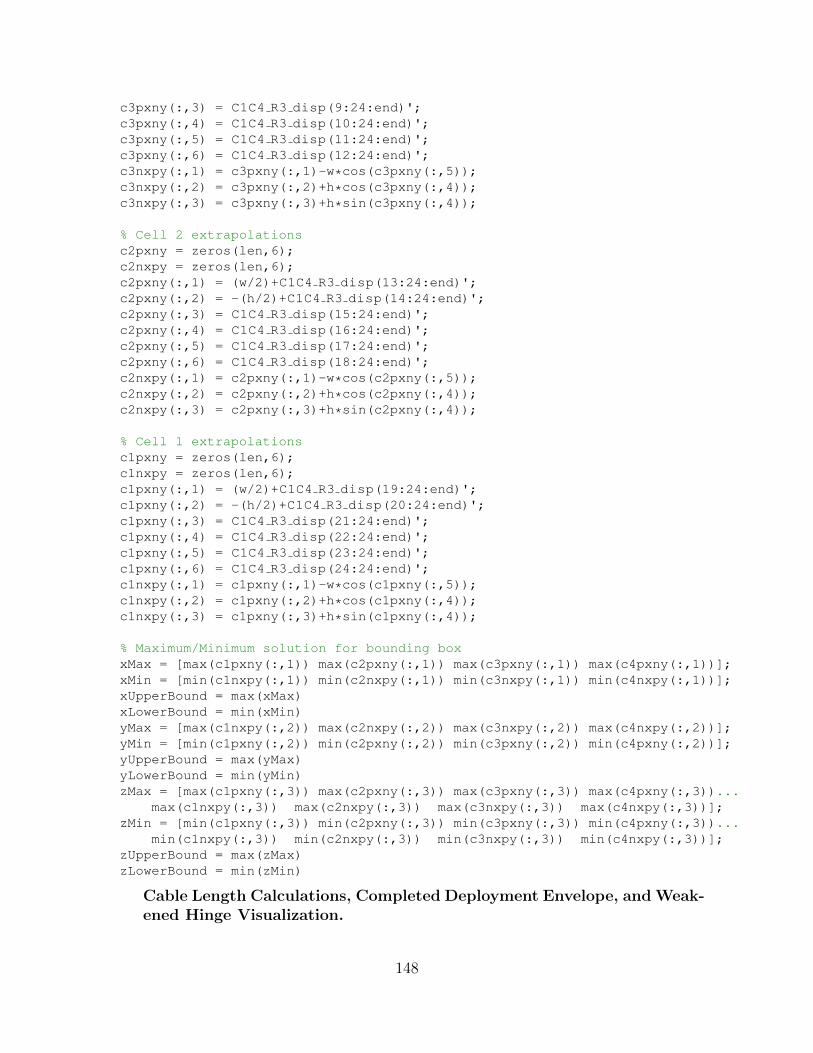
c3pxny(:,3) = C1C4 R3 disp(9:24:end)';c3pxny(:,4) = C1C4 R3 disp(10:24:end)';c3pxny(:,5) = C1C4 R3 disp(11:24:end)';c3pxny(:,6) = C1C4 R3 disp(12:24:end)';c3nxpy(:,1) = c3pxny(:,1)-w*cos(c3pxny(:,5));c3nxpy(:,2) = c3pxny(:,2)+h*cos(c3pxny(:,4));c3nxpy(:,3) = c3pxny(:,3)+h*sin(c3pxny(:,4));
% Cell 2 extrapolationsc2pxny = zeros(len,6);c2nxpy = zeros(len,6);c2pxny(:,1) = (w/2)+C1C4 R3 disp(13:24:end)';c2pxny(:,2) = -(h/2)+C1C4 R3 disp(14:24:end)';c2pxny(:,3) = C1C4 R3 disp(15:24:end)';c2pxny(:,4) = C1C4 R3 disp(16:24:end)';c2pxny(:,5) = C1C4 R3 disp(17:24:end)';c2pxny(:,6) = C1C4 R3 disp(18:24:end)';c2nxpy(:,1) = c2pxny(:,1)-w*cos(c2pxny(:,5));c2nxpy(:,2) = c2pxny(:,2)+h*cos(c2pxny(:,4));c2nxpy(:,3) = c2pxny(:,3)+h*sin(c2pxny(:,4));
% Cell 1 extrapolationsc1pxny = zeros(len,6);c1nxpy = zeros(len,6);c1pxny(:,1) = (w/2)+C1C4 R3 disp(19:24:end)';c1pxny(:,2) = -(h/2)+C1C4 R3 disp(20:24:end)';c1pxny(:,3) = C1C4 R3 disp(21:24:end)';c1pxny(:,4) = C1C4 R3 disp(22:24:end)';c1pxny(:,5) = C1C4 R3 disp(23:24:end)';c1pxny(:,6) = C1C4 R3 disp(24:24:end)';c1nxpy(:,1) = c1pxny(:,1)-w*cos(c1pxny(:,5));c1nxpy(:,2) = c1pxny(:,2)+h*cos(c1pxny(:,4));c1nxpy(:,3) = c1pxny(:,3)+h*sin(c1pxny(:,4));
% Maximum/Minimum solution for bounding boxxMax = [max(c1pxny(:,1)) max(c2pxny(:,1)) max(c3pxny(:,1)) max(c4pxny(:,1))];xMin = [min(c1nxpy(:,1)) min(c2nxpy(:,1)) min(c3nxpy(:,1)) min(c4nxpy(:,1))];xUpperBound = max(xMax)xLowerBound = min(xMin)yMax = [max(c1nxpy(:,2)) max(c2nxpy(:,2)) max(c3nxpy(:,2)) max(c4nxpy(:,2))];yMin = [min(c1pxny(:,2)) min(c2pxny(:,2)) min(c3pxny(:,2)) min(c4pxny(:,2))];yUpperBound = max(yMax)yLowerBound = min(yMin)zMax = [max(c1pxny(:,3)) max(c2pxny(:,3)) max(c3pxny(:,3)) max(c4pxny(:,3))...
max(c1nxpy(:,3)) max(c2nxpy(:,3)) max(c3nxpy(:,3)) max(c4nxpy(:,3))];zMin = [min(c1pxny(:,3)) min(c2pxny(:,3)) min(c3pxny(:,3)) min(c4pxny(:,3))...
min(c1nxpy(:,3)) min(c2nxpy(:,3)) min(c3nxpy(:,3)) min(c4nxpy(:,3))];zUpperBound = max(zMax)zLowerBound = min(zMin)
Cable Length Calculations, Completed Deployment Envelope, and Weak-ened Hinge Visualization.
148

%% Cable Lengths Calculations% Dylan Van Dyne 10 Dec 2014
clear all; clc; close all;
%% Calculating Cable Lengths% Assuming the desired resting tension for these cables is 10N, with 25% N/m spring constant, so the x0 is set to 0.2 meters. Setting back% corners of cells to 90 degrees with this method.
F = 10; % Desired forcek = 25; % Cable spring constantstr = F/k % Desired stretch in cables
vb = 5.310-0.0255; % Vertical batten length (adjusted for corners)hb = 8.74-.102; % Horizontal batten length (adjusted for corners)c1 top = 4.583*2; % Cell 1 top length (adjusted for joints)c1 bot = 4.7215*2; % Cell 1 bottom length (adjusted for joints)c1 nypy = sqrt(vbˆ2+c1 topˆ2)-strc1 pyny = sqrt(vbˆ2+c1 botˆ2)-strc1 py = sqrt(hbˆ2+c1 topˆ2)-strc1 ny = sqrt(hbˆ2+c1 botˆ2)-strc2 top = 4.598*2;c2 bot = 4.7385*2;c2 nypy = sqrt(vbˆ2+c2 topˆ2)-strc2 pyny = sqrt(vbˆ2+c2 botˆ2)-strc2 py = sqrt(hbˆ2+c2 topˆ2)-strc2 ny = sqrt(hbˆ2+c2 botˆ2)-strc3 top = 4.6285*2;c3 bot = 4.7725*2;c3 nypy = sqrt(vbˆ2+c3 topˆ2)-strc3 pyny = sqrt(vbˆ2+c3 botˆ2)-strc3 py = sqrt(hbˆ2+c3 topˆ2)-strc3 ny = sqrt(hbˆ2+c3 botˆ2)-strc4 top = 4.6735*2;c4 bot = 4.823*2;c4 nypy = sqrt(vbˆ2+c4 topˆ2)-strc4 pyny = sqrt(vbˆ2+c4 botˆ2)-strc4 py = sqrt(hbˆ2+c4 topˆ2)-strc4 ny = sqrt(hbˆ2+c4 botˆ2)-str
%% Determining Completed Geometry Envelopexmax = (8.74+.202)/2lg adj = 0.051; % Longeron cornertheta f1 = atand(vb/(c1 bot-c1 top)); % Forward angle of celltheta c1r = 90-theta f1; % Cell 1 raise anglec2 zdist = (lg adj+c2 bot)*cosd(theta c1r); % Adjusted y distance for Cell 2theta f2 = atand(vb/(c2 bot-c2 top));theta c2r = 90-theta f2+theta c1r;c3 zdist = (lg adj+c3 bot)*cosd(theta c2r);theta f3 = atand(vb/(c3 bot-c3 top));theta c3r = 90-theta f3+theta c2r+theta c1r;
149

c4 zdist = (lg adj+c4 bot)*cosd(theta c3r);c2 ydist = c2 top*sind(theta c1r);c3 ydist = c3 top*sind(theta c2r);c4 ydist = c4 top*sind(theta c3r);ymax = vb/2+c2 ydist+c3 ydist+c4 ydistzmax = c1 bot+c2 zdist+c3 zdist+c4 zdist
%% Draw Deployed Truss Armfigure;c1z = [0 0 c1 bot c1 top 0];c1y = [vb/2 -vb/2 -vb/2 vb/2 vb/2];c2 blx = c1 bot;c2 bly = -vb/2;c2 tlx = c1 top;c2 tly = vb/2;c2 trx = c1 top+c2 top*cosd(theta c1r);c2 try = vb/2+c2 top*sind(theta c1r);c2 brx = c1 bot+c2 bot*cosd(theta c1r);c2 bry = -vb/2+c2 bot*sind(theta c1r);c2z = [c2 blx c2 tlx c2 trx c2 brx c2 blx];c2y = [c2 bly c2 tly c2 try c2 bry c2 bly];c3 blx = c2 brx;c3 bly = c2 bry;c3 tlx = c2 trx;c3 tly = c2 try;c3 trx = c2 trx+c3 top*cosd(theta c2r);c3 try = c2 try+c3 top*sind(theta c2r);c3 brx = c2 brx+c3 bot*cosd(theta c2r);c3 bry = c2 bry+c3 bot*sind(theta c2r);c3z = [c3 blx c3 tlx c3 trx c3 brx c3 blx];c3y = [c3 bly c3 tly c3 try c3 bry c3 bly];c4 blx = c3 brx;c4 bly = c3 bry;c4 tlx = c3 trx;c4 tly = c3 try;c4 trx = c3 trx+c4 top*cosd(theta c3r);c4 try = c3 try+c4 top*sind(theta c3r);c4 brx = c3 brx+c4 bot*cosd(theta c3r);c4 bry = c3 bry+c4 bot*sind(theta c3r);c4z = [c4 blx c4 tlx c4 trx c4 brx c4 blx];c4y = [c4 bly c4 tly c4 try c4 bry c4 bly];% C1 Uppersubplot(4,2,1)hold ontitle('Weak Hinge in an Upper Longeron of Cell 1 (Success)')plot(c1z(1:2),c1y(1:2),'k')plot(c1z(4:5),c1y(4:5),':b')plot(c1z(3:4),c1y(3:4),'k')plot(c1z(2:3),c1y(2:3),'b')plot(c2z(2:3),c2y(2:3),'b')plot(c2z(3:4),c2y(3:4),'k')plot(c2z(4:5),c2y(4:5),'b','LineWidth',2)
150

plot(c3z(2:3),c3y(2:3),'b')plot(c3z(3:4),c3y(3:4),'k')plot(c3z(4:5),c3y(4:5),'b','LineWidth',3)plot(c4z(2:3),c4y(2:3),'b')plot(c4z(3:4),c4y(3:4),'k')plot(c4z(4:5),c4y(4:5),'b','LineWidth',6)axis('equal')axis([0 40 -5 10])xlabel('Z Axis (m)')ylabel('Y Axis (m)')hold off% C1 Lowersubplot(4,2,2)hold ontitle('Weak Hinge in a Lower Longeron of Cell 1 (Fail)')plot(c1z(1:2),c1y(1:2),'k')plot(c1z(4:5),c1y(4:5),'r')plot(c1z(3:4),c1y(3:4),'k')plot(c1z(2:3),c1y(2:3),':r')plot(c2z(2:3),c2y(2:3),'r')plot(c2z(3:4),c2y(3:4),'k')plot(c2z(4:5),c2y(4:5),'r','LineWidth',2)plot(c3z(2:3),c3y(2:3),'r')plot(c3z(3:4),c3y(3:4),'k')plot(c3z(4:5),c3y(4:5),'r','LineWidth',3)plot(c4z(2:3),c4y(2:3),'r')plot(c4z(3:4),c4y(3:4),'k')plot(c4z(4:5),c4y(4:5),'w')axis('equal')axis([0 40 -5 10])xlabel('Z Axis (m)')ylabel('Y Axis (m)')hold off% C2 Uppersubplot(4,2,3)hold ontitle('Weak Hinge in an Upper Longeron of Cell 2 (Fail)')plot(c1z(1:2),c1y(1:2),'k')plot(c1z(4:5),c1y(4:5),'r')plot(c1z(3:4),c1y(3:4),'k')plot(c1z(2:3),c1y(2:3),'r')plot(c2z(2:3),c2y(2:3),':r','LineWidth',2)plot(c2z(3:4),c2y(3:4),'k')plot(c2z(4:5),c2y(4:5),'r')plot(c3z(2:3),c3y(2:3),'r')plot(c3z(3:4),c3y(3:4),'k')plot(c3z(4:5),c3y(4:5),'r','LineWidth',3)plot(c4z(2:3),c4y(2:3),'r')plot(c4z(3:4),c4y(3:4),'k')plot(c4z(4:5),c4y(4:5),'w')axis('equal')axis([0 40 -5 10])
151

xlabel('Z Axis (m)')ylabel('Y Axis (m)')hold off% C2 Lowersubplot(4,2,4)hold ontitle('Weak Hinge in a Lower Longeron of Cell 2 (Fail)')plot(c1z(1:2),c1y(1:2),'k')plot(c1z(4:5),c1y(4:5),'w')plot(c1z(3:4),c1y(3:4),'k')plot(c1z(2:3),c1y(2:3),'r')plot(c2z(2:3),c2y(2:3),'r')plot(c2z(3:4),c2y(3:4),'k')plot(c2z(4:5),c2y(4:5),':r','LineWidth',2)plot(c3z(2:3),c3y(2:3),'r','LineWidth',2)plot(c3z(3:4),c3y(3:4),'k')plot(c3z(4:5),c3y(4:5),'r','LineWidth',4)plot(c4z(2:3),c4y(2:3),'r')plot(c4z(3:4),c4y(3:4),'k')plot(c4z(4:5),c4y(4:5),'w')axis('equal')axis([0 40 -5 10])xlabel('Z Axis (m)')ylabel('Y Axis (m)')hold off% C3 Uppersubplot(4,2,5)hold ontitle('Weak Hinge in an Upper Longeron of Cell 3 (Success)')plot(c1z(1:2),c1y(1:2),'k')plot(c1z(4:5),c1y(4:5),'b')plot(c1z(3:4),c1y(3:4),'k')plot(c1z(2:3),c1y(2:3),'b')plot(c2z(2:3),c2y(2:3),'b')plot(c2z(3:4),c2y(3:4),'k')plot(c2z(4:5),c2y(4:5),'b','LineWidth',2)plot(c3z(2:3),c3y(2:3),':b','LineWidth',2)plot(c3z(3:4),c3y(3:4),'k')plot(c3z(4:5),c3y(4:5),'b')plot(c4z(2:3),c4y(2:3),'b')plot(c4z(3:4),c4y(3:4),'k')plot(c4z(4:5),c4y(4:5),'b','LineWidth',6)axis('equal')axis([0 40 -5 10])xlabel('Z Axis (m)')ylabel('Y Axis (m)')hold off% C3 Lowersubplot(4,2,6)hold ontitle('Weak Hinge in a Lower Longeron of Cell 3 (Success)')plot(c1z(1:2),c1y(1:2),'k')
152

plot(c1z(4:5),c1y(4:5),'b')plot(c1z(3:4),c1y(3:4),'k')plot(c1z(2:3),c1y(2:3),'b')plot(c2z(2:3),c2y(2:3),'b')plot(c2z(3:4),c2y(3:4),'k')plot(c2z(4:5),c2y(4:5),'b')plot(c3z(2:3),c3y(2:3),'b')plot(c3z(3:4),c3y(3:4),'k')plot(c3z(4:5),c3y(4:5),':b','LineWidth',3)plot(c4z(2:3),c4y(2:3),'b')plot(c4z(3:4),c4y(3:4),'k')plot(c4z(4:5),c4y(4:5),'b')axis('equal')axis([0 40 -5 10])xlabel('Z Axis (m)')ylabel('Y Axis (m)')hold off% C4 Uppersubplot(4,2,7)hold ontitle('Weak Hinge in an Upper Longeron of Cell 4 (Success)')plot(c1z(1:2),c1y(1:2),'k')plot(c1z(4:5),c1y(4:5),'b')plot(c1z(3:4),c1y(3:4),'k')plot(c1z(2:3),c1y(2:3),'b')plot(c2z(2:3),c2y(2:3),'b')plot(c2z(3:4),c2y(3:4),'k')plot(c2z(4:5),c2y(4:5),'b','LineWidth',2)plot(c3z(2:3),c3y(2:3),'b')plot(c3z(3:4),c3y(3:4),'k')plot(c3z(4:5),c3y(4:5),'b','LineWidth',4)plot(c4z(2:3),c4y(2:3),':b','LineWidth',4)plot(c4z(3:4),c4y(3:4),'k')plot(c4z(4:5),c4y(4:5),'b')axis('equal')axis([0 40 -5 10])xlabel('Z Axis (m)')ylabel('Y Axis (m)')hold off% C4 Lowersubplot(4,2,8)hold ontitle('Weak Hinge in a Lower Longeron of Cell 4 (Fail)')plot(c1z(1:2),c1y(1:2),'k')plot(c1z(4:5),c1y(4:5),'r')plot(c1z(3:4),c1y(3:4),'k')plot(c1z(2:3),c1y(2:3),'r')plot(c2z(2:3),c2y(2:3),'r')plot(c2z(3:4),c2y(3:4),'k')plot(c2z(4:5),c2y(4:5),'r','LineWidth',2)plot(c3z(2:3),c3y(2:3),'r')plot(c3z(3:4),c3y(3:4),'k')
153

plot(c3z(4:5),c3y(4:5),'r','LineWidth',3)plot(c4z(2:3),c4y(2:3),'r')plot(c4z(3:4),c4y(3:4),'k')plot(c4z(4:5),c4y(4:5),'w')axis('equal')axis([0 40 -5 10])xlabel('Z Axis (m)')ylabel('Y Axis (m)')hold off
6.2 Appendix B - Simulation Import Files Examples
Simulation Parameter Input File.
ks 5 Spring Constantthl 3.14 Locking Anglek 50 Cable Spring Constantc 5 Cable Damping Constantl.c1.nypy 10.3802l.c1.pyny 10.6211l.c1.py 12.3949l.c1.ny 12.5979l.c2.nypy 10.4062l.c2.pyny 10.6508l.c2.py 12.4167l.c2.ny 12.6230l.c3.nypy 10.4592l.c3.pyny 10.7102l.c3.py 12.4612l.c3.ny 12.6733l.c4.nypy 10.5374l.c4.pyny 10.7987l.c4.py 12.5272l.c4.ny 12.7484
Truss Cell 1 Cable File.
mbd.dsj1.xsx mbd.att6.xcxmbd.dsj1.xsy mbd.att6.xcymbd.dsj1.xsz mbd.att6.xczmbd.dsj1.xdx mbd.att7.xcxmbd.dsj1.xdy mbd.att7.xcymbd.dsj1.xdz mbd.att7.xczmbd.dsj1.uc.src mbd.att6.umbd.dsj1.vc.src mbd.att6.v
154

mbd.dsj1.wc.src mbd.att6.wmbd.dsj1.uc.dest mbd.att7.umbd.dsj1.vc.dest mbd.att7.vmbd.dsj1.wc.dest mbd.att7.wc1.NXnypy.dist sqrt((mbd.dsj1.xsx+mbd.dsj1.uc.src-mbd.dsj1.xdx-mbd.dsj1.uc.dest)ˆ2+(mbd.dsj1.xsy+mbd.dsj1.vc.src-mbd.dsj1.xdy-mbd.dsj1.vc.dest)ˆ2+(mbd.dsj1.xsz+mbd.dsj1.wc.src-mbd.dsj1.xdz-mbd.dsj1.wc.dest)ˆ2+eps)c1.NXnypy.distx (mbd.dsj1.xsx+mbd.dsj1.uc.src-mbd.dsj1.xdx-mbd.dsj1.uc.dest)/c1.NXnypy.distc1.NXnypy.disty (mbd.dsj1.xsy+mbd.dsj1.vc.src-mbd.dsj1.xdy-mbd.dsj1.vc.dest)/c1.NXnypy.distc1.NXnypy.distz (mbd.dsj1.xsz+mbd.dsj1.wc.src-mbd.dsj1.xdz-mbd.dsj1.wc.dest)/c1.NXnypy.distc1.NXnypy.damp d(c1.NXnypy.dist,TIME)c1.NXnypy.sw c1.NXnypy.dist¿l.c1.nypyc1.NXnypy.f (k*(l.c1.nypy-c1.NXnypy.dist)-c*(c1.NXnypy.damp¿0)*c1.NXnypy.damp)*c1.NXnypy.swc1.NXnypy.Ws c1.NXnypy.sw*.5*k*(l.c1.nypy-c1.NXnypy.dist)ˆ2c1.NXnypy.fx c1.NXnypy.f*c1.NXnypy.distxc1.NXnypy.fy c1.NXnypy.f*c1.NXnypy.distyc1.NXnypy.fz c1.NXnypy.f*c1.NXnypy.distzmbd.dsj2.xsx mbd.att12.xcxmbd.dsj2.xsy mbd.att12.xcymbd.dsj2.xsz mbd.att12.xczmbd.dsj2.xdx mbd.att1.xcxmbd.dsj2.xdy mbd.att1.xcymbd.dsj2.xdz mbd.att1.xczmbd.dsj2.uc.src mbd.att12.umbd.dsj2.vc.src mbd.att12.vmbd.dsj2.wc.src mbd.att12.wmbd.dsj2.uc.dest mbd.att1.umbd.dsj2.vc.dest mbd.att1.vmbd.dsj2.wc.dest mbd.att1.wc1.NXpyny.dist sqrt((mbd.dsj2.xsx+mbd.dsj2.uc.src-mbd.dsj2.xdx-mbd.dsj2.uc.dest)ˆ2+(mbd.dsj2.xsy+mbd.dsj2.vc.src-mbd.dsj2.xdy-mbd.dsj2.vc.dest)ˆ2+(mbd.dsj2.xsz+mbd.dsj2.wc.src-mbd.dsj2.xdz-mbd.dsj2.wc.dest)ˆ2+eps)c1.NXpyny.distx (mbd.dsj2.xsx+mbd.dsj2.uc.src-mbd.dsj2.xdx-mbd.dsj2.uc.dest)/c1.NXpyny.distc1.NXpyny.disty (mbd.dsj2.xsy+mbd.dsj2.vc.src-mbd.dsj2.xdy-mbd.dsj2.vc.dest)/c1.NXpyny.distc1.NXpyny.distz (mbd.dsj2.xsz+mbd.dsj2.wc.src-mbd.dsj2.xdz-mbd.dsj2.wc.dest)/c1.NXpyny.distc1.NXpyny.damp d(c1.NXpyny.dist,TIME)
155

c1.NXpyny.sw c1.NXpyny.dist¿l.c1.pynyc1.NXpyny.f (k*(l.c1.pyny-c1.NXpyny.dist)-c*(c1.NXpyny.damp¿0)*c1.NXpyny.damp)*c1.NXpyny.swc1.NXpyny.Ws c1.NXpyny.sw*.5*k*(l.c1.pyny-c1.NXpyny.dist)ˆ2c1.NXpyny.fx c1.NXpyny.f*c1.NXpyny.distxc1.NXpyny.fy c1.NXpyny.f*c1.NXpyny.distyc1.NXpyny.fz c1.NXpyny.f*c1.NXpyny.distzmbd.dsj3.xsx mbd.att18.xcxmbd.dsj3.xsy mbd.att18.xcymbd.dsj3.xsz mbd.att18.xczmbd.dsj3.xdx mbd.att19.xcxmbd.dsj3.xdy mbd.att19.xcymbd.dsj3.xdz mbd.att19.xczmbd.dsj3.uc.src mbd.att18.umbd.dsj3.vc.src mbd.att18.vmbd.dsj3.wc.src mbd.att18.wmbd.dsj3.uc.dest mbd.att19.umbd.dsj3.vc.dest mbd.att19.vmbd.dsj3.wc.dest mbd.att19.wc1.PXnypy.dist sqrt((mbd.dsj3.xsx+mbd.dsj3.uc.src-mbd.dsj3.xdx-mbd.dsj3.uc.dest)ˆ2+(mbd.dsj3.xsy+mbd.dsj3.vc.src-mbd.dsj3.xdy-mbd.dsj3.vc.dest)ˆ2+(mbd.dsj3.xsz+mbd.dsj3.wc.src-mbd.dsj3.xdz-mbd.dsj3.wc.dest)ˆ2+eps)c1.PXnypy.distx (mbd.dsj3.xsx+mbd.dsj3.uc.src-mbd.dsj3.xdx-mbd.dsj3.uc.dest)/c1.PXnypy.distc1.PXnypy.disty (mbd.dsj3.xsy+mbd.dsj3.vc.src-mbd.dsj3.xdy-mbd.dsj3.vc.dest)/c1.PXnypy.distc1.PXnypy.distz (mbd.dsj3.xsz+mbd.dsj3.wc.src-mbd.dsj3.xdz-mbd.dsj3.wc.dest)/c1.PXnypy.distc1.PXnypy.damp d(c1.PXnypy.dist,TIME)c1.PXnypy.sw c1.PXnypy.dist¿l.c1.nypyc1.PXnypy.f (k*(l.c1.nypy-c1.PXnypy.dist)-c*(c1.PXnypy.damp¿0)*c1.PXnypy.damp)*c1.PXnypy.swc1.PXnypy.Ws c1.PXnypy.sw*.5*k*(l.c1.nypy-c1.PXnypy.dist)ˆ2c1.PXnypy.fx c1.PXnypy.f*c1.PXnypy.distxc1.PXnypy.fy c1.PXnypy.f*c1.PXnypy.distyc1.PXnypy.fz c1.PXnypy.f*c1.PXnypy.distzmbd.dsj4.xsx mbd.att24.xcxmbd.dsj4.xsy mbd.att24.xcymbd.dsj4.xsz mbd.att24.xczmbd.dsj4.xdx mbd.att13.xcxmbd.dsj4.xdy mbd.att13.xcymbd.dsj4.xdz mbd.att13.xczmbd.dsj4.uc.src mbd.att24.u
156

mbd.dsj4.vc.src mbd.att24.vmbd.dsj4.wc.src mbd.att24.wmbd.dsj4.uc.dest mbd.att13.umbd.dsj4.vc.dest mbd.att13.vmbd.dsj4.wc.dest mbd.att13.wc1.PXpyny.dist sqrt((mbd.dsj4.xsx+mbd.dsj4.uc.src-mbd.dsj4.xdx-mbd.dsj4.uc.dest)ˆ2+(mbd.dsj4.xsy+mbd.dsj4.vc.src-mbd.dsj4.xdy-mbd.dsj4.vc.dest)ˆ2+(mbd.dsj4.xsz+mbd.dsj4.wc.src-mbd.dsj4.xdz-mbd.dsj4.wc.dest)ˆ2+eps)c1.PXpyny.distx (mbd.dsj4.xsx+mbd.dsj4.uc.src-mbd.dsj4.xdx-mbd.dsj4.uc.dest)/c1.PXpyny.distc1.PXpyny.disty (mbd.dsj4.xsy+mbd.dsj4.vc.src-mbd.dsj4.xdy-mbd.dsj4.vc.dest)/c1.PXpyny.distc1.PXpyny.distz (mbd.dsj4.xsz+mbd.dsj4.wc.src-mbd.dsj4.xdz-mbd.dsj4.wc.dest)/c1.PXpyny.distc1.PXpyny.damp d(c1.PXpyny.dist,TIME)c1.PXpyny.sw c1.PXpyny.dist¿l.c1.pynyc1.PXpyny.f (k*(l.c1.pyny-c1.PXpyny.dist)-c*(c1.PXpyny.damp¿0)*c1.PXpyny.damp)*c1.PXpyny.swc1.PXpyny.Ws c1.PXpyny.sw*.5*k*(l.c1.pyny-c1.PXpyny.dist)ˆ2c1.PXpyny.fx c1.PXpyny.f*c1.PXpyny.distxc1.PXpyny.fy c1.PXpyny.f*c1.PXpyny.distyc1.PXpyny.fz c1.PXpyny.f*c1.PXpyny.distzmbd.dsj5.xsx mbd.att18.xcxmbd.dsj5.xsy mbd.att18.xcymbd.dsj5.xsz mbd.att18.xczmbd.dsj5.xdx mbd.att1.xcxmbd.dsj5.xdy mbd.att1.xcymbd.dsj5.xdz mbd.att1.xczmbd.dsj5.uc.src mbd.att18.umbd.dsj5.vc.src mbd.att18.vmbd.dsj5.wc.src mbd.att18.wmbd.dsj5.uc.dest mbd.att1.umbd.dsj5.vc.dest mbd.att1.vmbd.dsj5.wc.dest mbd.att1.wc1.nxpxPY.dist sqrt((mbd.dsj5.xsx+mbd.dsj5.uc.src-mbd.dsj5.xdx-mbd.dsj5.uc.dest)ˆ2+(mbd.dsj5.xsy+mbd.dsj5.vc.src-mbd.dsj5.xdy-mbd.dsj5.vc.dest)ˆ2+(mbd.dsj5.xsz+mbd.dsj5.wc.src-mbd.dsj5.xdz-mbd.dsj5.wc.dest)ˆ2+eps)c1.nxpxPY.distx (mbd.dsj5.xsx+mbd.dsj5.uc.src-mbd.dsj5.xdx-mbd.dsj5.uc.dest)/c1.nxpxPY.distc1.nxpxPY.disty (mbd.dsj5.xsy+mbd.dsj5.vc.src-mbd.dsj5.xdy-mbd.dsj5.vc.dest)/c1.nxpxPY.distc1.nxpxPY.distz (mbd.dsj5.xsz+mbd.dsj5.wc.src-mbd.dsj5.xdz-mbd.dsj5.wc.dest)/c1.nxpxPY.dist
157

c1.nxpxPY.damp d(c1.nxpxPY.dist,TIME)c1.nxpxPY.sw c1.nxpxPY.dist¿l.c1.pyc1.nxpxPY.f (k*(l.c1.py-c1.nxpxPY.dist)-c*(c1.nxpxPY.damp¿0)*c1.nxpxPY.damp)*c1.nxpxPY.swc1.nxpxPY.Ws c1.nxpxPY.sw*.5*k*(l.c1.py-c1.nxpxPY.dist)ˆ2c1.nxpxPY.fx c1.nxpxPY.f*c1.nxpxPY.distxc1.nxpxPY.fy c1.nxpxPY.f*c1.nxpxPY.distyc1.nxpxPY.fz c1.nxpxPY.f*c1.nxpxPY.distzmbd.dsj6.xsx mbd.att6.xcxmbd.dsj6.xsy mbd.att6.xcymbd.dsj6.xsz mbd.att6.xczmbd.dsj6.xdx mbd.att13.xcxmbd.dsj6.xdy mbd.att13.xcymbd.dsj6.xdz mbd.att13.xczmbd.dsj6.uc.src mbd.att6.umbd.dsj6.vc.src mbd.att6.vmbd.dsj6.wc.src mbd.att6.wmbd.dsj6.uc.dest mbd.att13.umbd.dsj6.vc.dest mbd.att13.vmbd.dsj6.wc.dest mbd.att13.wc1.pxnxPY.dist sqrt((mbd.dsj6.xsx+mbd.dsj6.uc.src-mbd.dsj6.xdx-mbd.dsj6.uc.dest)ˆ2+(mbd.dsj6.xsy+mbd.dsj6.vc.src-mbd.dsj6.xdy-mbd.dsj6.vc.dest)ˆ2+(mbd.dsj6.xsz+mbd.dsj6.wc.src-mbd.dsj6.xdz-mbd.dsj6.wc.dest)ˆ2+eps)c1.pxnxPY.distx (mbd.dsj6.xsx+mbd.dsj6.uc.src-mbd.dsj6.xdx-mbd.dsj6.uc.dest)/c1.pxnxPY.distc1.pxnxPY.disty (mbd.dsj6.xsy+mbd.dsj6.vc.src-mbd.dsj6.xdy-mbd.dsj6.vc.dest)/c1.pxnxPY.distc1.pxnxPY.distz (mbd.dsj6.xsz+mbd.dsj6.wc.src-mbd.dsj6.xdz-mbd.dsj6.wc.dest)/c1.pxnxPY.distc1.pxnxPY.damp d(c1.pxnxPY.dist,TIME)c1.pxnxPY.sw c1.pxnxPY.dist¿l.c1.pyc1.pxnxPY.f (k*(l.c1.py-c1.pxnxPY.dist)-c*(c1.pxnxPY.damp¿0)*c1.pxnxPY.damp)*c1.pxnxPY.swc1.pxnxPY.Ws c1.pxnxPY.sw*.5*k*(l.c1.py-c1.pxnxPY.dist)ˆ2c1.pxnxPY.fx c1.pxnxPY.f*c1.pxnxPY.distxc1.pxnxPY.fy c1.pxnxPY.f*c1.pxnxPY.distyc1.pxnxPY.fz c1.pxnxPY.f*c1.pxnxPY.distzmbd.dsj7.xsx mbd.att24.xcxmbd.dsj7.xsy mbd.att24.xcymbd.dsj7.xsz mbd.att24.xczmbd.dsj7.xdx mbd.att7.xcxmbd.dsj7.xdy mbd.att7.xcymbd.dsj7.xdz mbd.att7.xcz
158

mbd.dsj7.uc.src mbd.att24.umbd.dsj7.vc.src mbd.att24.vmbd.dsj7.wc.src mbd.att24.wmbd.dsj7.uc.dest mbd.att7.umbd.dsj7.vc.dest mbd.att7.vmbd.dsj7.wc.dest mbd.att7.wc1.nxpxNY.dist sqrt((mbd.dsj7.xsx+mbd.dsj7.uc.src-mbd.dsj7.xdx-mbd.dsj7.uc.dest)ˆ2+(mbd.dsj7.xsy+mbd.dsj7.vc.src-mbd.dsj7.xdy-mbd.dsj7.vc.dest)ˆ2+(mbd.dsj7.xsz+mbd.dsj7.wc.src-mbd.dsj7.xdz-mbd.dsj7.wc.dest)ˆ2+eps)c1.nxpxNY.distx (mbd.dsj7.xsx+mbd.dsj7.uc.src-mbd.dsj7.xdx-mbd.dsj7.uc.dest)/c1.nxpxNY.distc1.nxpxNY.disty (mbd.dsj7.xsy+mbd.dsj7.vc.src-mbd.dsj7.xdy-mbd.dsj7.vc.dest)/c1.nxpxNY.distc1.nxpxNY.distz (mbd.dsj7.xsz+mbd.dsj7.wc.src-mbd.dsj7.xdz-mbd.dsj7.wc.dest)/c1.nxpxNY.distc1.nxpxNY.damp d(c1.nxpxNY.dist,TIME)c1.nxpxNY.sw c1.nxpxNY.dist¿l.c1.nyc1.nxpxNY.f (k*(l.c1.ny-c1.nxpxNY.dist)-c*(c1.nxpxNY.damp¿0)*c1.nxpxNY.damp)*c1.nxpxNY.swc1.nxpxNY.Ws c1.nxpxNY.sw*.5*k*(l.c1.ny-c1.nxpxNY.dist)ˆ2c1.nxpxNY.fx c1.nxpxNY.f*c1.nxpxNY.distxc1.nxpxNY.fy c1.nxpxNY.f*c1.nxpxNY.distyc1.nxpxNY.fz c1.nxpxNY.f*c1.nxpxNY.distzmbd.dsj8.xsx mbd.att12.xcxmbd.dsj8.xsy mbd.att12.xcymbd.dsj8.xsz mbd.att12.xczmbd.dsj8.xdx mbd.att19.xcxmbd.dsj8.xdy mbd.att19.xcymbd.dsj8.xdz mbd.att19.xczmbd.dsj8.uc.src mbd.att12.umbd.dsj8.vc.src mbd.att12.vmbd.dsj8.wc.src mbd.att12.wmbd.dsj8.uc.dest mbd.att19.umbd.dsj8.vc.dest mbd.att19.vmbd.dsj8.wc.dest mbd.att19.wc1.pxnxNY.dist sqrt((mbd.dsj8.xsx+mbd.dsj8.uc.src-mbd.dsj8.xdx-mbd.dsj8.uc.dest)ˆ2+(mbd.dsj8.xsy+mbd.dsj8.vc.src-mbd.dsj8.xdy-mbd.dsj8.vc.dest)ˆ2+(mbd.dsj8.xsz+mbd.dsj8.wc.src-mbd.dsj8.xdz-mbd.dsj8.wc.dest)ˆ2+eps)c1.pxnxNY.distx (mbd.dsj8.xsx+mbd.dsj8.uc.src-mbd.dsj8.xdx-mbd.dsj8.uc.dest)/c1.pxnxNY.distc1.pxnxNY.disty (mbd.dsj8.xsy+mbd.dsj8.vc.src-mbd.dsj8.xdy-mbd.dsj8.vc.dest)/c1.pxnxNY.distc1.pxnxNY.distz (mbd.dsj8.xsz+mbd.dsj8.wc.src-mbd.dsj8.xdz-mbd.dsj8.wc.dest)
159

/c1.pxnxNY.distc1.pxnxNY.damp d(c1.pxnxNY.dist,TIME)c1.pxnxNY.sw c1.pxnxNY.dist¿l.c1.nyc1.pxnxNY.f (k*(l.c1.ny-c1.pxnxNY.dist)-c*(c1.pxnxNY.damp¿0)*c1.pxnxNY.damp)*c1.pxnxNY.swc1.pxnxNY.Ws c1.pxnxNY.sw*.5*k*(l.c1.ny-c1.pxnxNY.dist)ˆ2c1.pxnxNY.fx c1.pxnxNY.f*c1.pxnxNY.distxc1.pxnxNY.fy c1.pxnxNY.f*c1.pxnxNY.distyc1.pxnxNY.fz c1.pxnxNY.f*c1.pxnxNY.distzc1.tot.Ws c1.NXnypy.Ws+c1.NXpyny.Ws+c1.PXnypy.Ws+c1.PXpyny.Ws+c1.nxpxPY.Ws+c1.pxnxPY.Ws+c1.nxpxNY.Ws+c1.pxnxNY.Ws
160

REPORT DOCUMENTATION PAGE Form ApprovedOMB No. 0704–0188
The public reporting burden for this collection of information is estimated to average 1 hour per response, including the time for reviewing instructions, searching existing data sources, gathering andmaintaining the data needed, and completing and reviewing the collection of information. Send comments regarding this burden estimate or any other aspect of this collection of information, includingsuggestions for reducing this burden to Department of Defense, Washington Headquarters Services, Directorate for Information Operations and Reports (0704–0188), 1215 Jefferson Davis Highway,Suite 1204, Arlington, VA 22202–4302. Respondents should be aware that notwithstanding any other provision of law, no person shall be subject to any penalty for failing to comply with a collectionof information if it does not display a currently valid OMB control number. PLEASE DO NOT RETURN YOUR FORM TO THE ABOVE ADDRESS.
1. REPORT DATE (DD–MM–YYYY) 2. REPORT TYPE 3. DATES COVERED (From — To)
4. TITLE AND SUBTITLE 5a. CONTRACT NUMBER
5b. GRANT NUMBER
5c. PROGRAM ELEMENT NUMBER
5d. PROJECT NUMBER
5e. TASK NUMBER
5f. WORK UNIT NUMBER
6. AUTHOR(S)
7. PERFORMING ORGANIZATION NAME(S) AND ADDRESS(ES) 8. PERFORMING ORGANIZATION REPORTNUMBER
9. SPONSORING / MONITORING AGENCY NAME(S) AND ADDRESS(ES) 10. SPONSOR/MONITOR’S ACRONYM(S)
11. SPONSOR/MONITOR’S REPORTNUMBER(S)
12. DISTRIBUTION / AVAILABILITY STATEMENT
13. SUPPLEMENTARY NOTES
14. ABSTRACT
15. SUBJECT TERMS
16. SECURITY CLASSIFICATION OF:
a. REPORT b. ABSTRACT c. THIS PAGE
17. LIMITATION OFABSTRACT
18. NUMBEROFPAGES
19a. NAME OF RESPONSIBLE PERSON
19b. TELEPHONE NUMBER (include area code)
Standard Form 298 (Rev. 8–98)Prescribed by ANSI Std. Z39.18
26–03–2015 Master’s Thesis Oct 2013 — Mar 2015
Simulation of Locking Space Truss Deployments for a Large DeployableSparse Aperture Reflector
JON157454B
Van Dyne, Dylan M.
Air Force Institute of TechnologyGraduate School of Engineering and Management2950 Hobson WayWPAFB OH 45433-7765
AFIT-ENY-MS-15-M-250
Dr. David S. StargelChief, Dynamics Systems and ControlAir Force Office of Scientific Research875 N. Randolph St., Suite 325, Room 3112Arlington, VA 22203-1768Email: [email protected]
AFOSR/RTA
Distribution Statement A:Approved for Public Release; Distribution Unlimited.
This work is declared a work of the U.S. Government and is not subject to copyright protection in the United States.
Large deployable space structures require an inordinate amount of effort to fully design and test on Earth. To aid in the determination of the feasibility ofthe reflector, a method to simulate the structure’s deployment was developed using COMSOL. The simulation model is comprised of a locking hinge truss thatconstitutes the partial reflector structure. To meet computational and temporal restrictions, the structure is simplified to use simple beams with square crosssections and is meshed to a sufficient accuracy with second order elements. The geometry is modeled in the truss’s stowed configuration, with the connectinghinges and applied forces created via constraint equations in COMSOL. Many different simulations were run with varied design parameters in order todemonstrate the global motion of the deploying truss under differing conditions and to also showcase the capabilities of COMSOL’s implicit solver. It wasfound through all of the simulation variations that the success of the truss’s deployment is largely dependent on the condition of the lower truss members aswell as the interaction between the spring-loaded hinges and tension cables. The results demonstrate how COMSOL can be used to aid in the advancement ofthe Large Deployable Space Aperture Reflector design.
Space Structure, COMSOL, Multi-body-dynamics, Finite element analysis, Structure deployment
U U U UU 185
Dr. Alan Jennings, AFIT/ENY
(937) 255-3636, x7495; [email protected]