warwick.ac.uk/lib-publications

Original citation: Gaylard, A. P., Kabanovs, A., Jilesen, J., Kirwan, Kerry and Lockerby, Duncan A.. (2017) Simulation of rear surface contamination for a simple bluff body. Journal of Wind Engineering and Industrial Aerodynamics, 165. pp. 13-22. Permanent WRAP URL: http://wrap.warwick.ac.uk/86817 Copyright and reuse: The Warwick Research Archive Portal (WRAP) makes this work of researchers of the University of Warwick available open access under the following conditions. This article is made available under the Creative Commons Attribution 4.0 International license (CC BY 4.0) and may be reused according to the conditions of the license. For more details see: http://creativecommons.org/licenses/by/4.0/ A note on versions: The version presented in WRAP is the published version, or, version of record, and may be cited as it appears here. For more information, please contact the WRAP Team at: wrap@warwick.ac.uk

Contents lists available at ScienceDirect

Journal of Wind Engineeringand Industrial Aerodynamics

journal homepage: www.elsevier.com/locate/jweia

Simulation of rear surface contamination for a simple bluff body

A.P. Gaylarda,b,⁎, A. Kabanovsc, J. Jilesend, K. Kirwane, D.A. Lockerbyf

a Jaguar Land Rover, Banbury Road, Gaydon, Warwick CV35 ORR, UKb WMG, International Manufacturing Centre, University of Warwick, Coventry CV4 7AL, UKc Aeronautical and Automotive Engineering, Loughborough University, Leicestershire LE11 3TU, UKd Exa Corporation, 55 Network Dr, Burlington, MA 01803, USAe WMG, International Manufacturing Centre, University of Warwick, Coventry CV4 7AL, UKf School of Engineering, University of Warwick, Coventry CV4 7AL, UK

A R T I C L E I N F O

Keywords:CFDVLESAerodynamicsSurface contaminationWindsor bodyLattice Boltzmann

A B S T R A C T

Predicting the accumulation of material on the rear surfaces of square-backed cars is important to vehiclemanufacturers, as this progressively compromises rear vision, vehicle visibility and aesthetics. It also reducesthe effectiveness of rear mounted cameras. Here, this problem is represented by a simple bluff body with a singlesprayer mounted centrally under its rear trailing edge.

A Very Large Eddy Simulation (VLES) solver is used to simulate both the aerodynamics of the body anddeposition of contaminant. Aerodynamic drag and lift coefficients were predicted to within +1.3% and −4.2% oftheir experimental values, respectively. Wake topology was also correctly captured, resulting in a credibleprediction of the rear surface deposition pattern.

Contaminant deposition is mainly driven by the lower part of the wake ring vortex, which advects materialback onto the rear surface. This leads to a maximum below the rear stagnation point and an association withregions of higher base pressure.

The accumulation of mass is linear with time; the relative distribution changing little as the simulationprogresses, implying that shorter simulations can be compared to longer experiments. Further, the rate ofaccumulation quickly reaches a settled mean value, suggesting utility as a metric for assessing different vehicles.

1. Introduction

The following presents a numerical simulation of rear surfacecontamination for a simple bluff body, representing a road vehicle. Itexplores the interaction of an idealised tyre spray with a vehicle basewake and the resulting accumulation of material on the rear surface.

This models a significant issue: the accumulation of contaminants(soil, tyre debris, etc.) on the rear surfaces of cars diminishes bothdrivers’ vision and vehicle visibility as material is deposited on lightsand the rear screen. In addition, the aesthetic appeal of the vehicle maybe reduced and soil transferred to users’ hands and clothes as theyaccess the rear load space via the tailgate. These processes have thepotential to undermine customers’ perceptions of product quality(Gaylard et al., 2014).

The main contaminant source for these surfaces is the spraygenerated by the vehicle's own rear tyres, as they move over wet road(Jilesen et al., 2013). This is advected into the base wake andsubsequently deposited onto the vehicle's rear surfaces. The coupling

with wake flows, and hence vehicle aerodynamic performance, meansthat this issue must be addressed concurrently with aerodynamic dragduring the development process.

It has long been appreciated that square-backed vehicles such ashatchbacks, estates, and SUVs are particularly susceptible to this issue(Maycock, 1966) along with bus bodies (Lajos et al., 1986). Thereforethis work uses a square-backed bluff body to represent vulnerable cardesigns.

Simplified bodies, which represent a few salient geometric features,are widely used in automotive aerodynamics, for an overview of thispractise see Le Good and Garry (2004). They enable key processes to beinvestigated without the myriad interactions seen in productionvehicles, or having to cope with their geometric complexity. In essence,they provide an improved signal-to-noise ratio, by omitting geometryresponsible for generating flow features not significant for the class ofproblem under investigation.

However, this potentially useful approach has yet to be widelyapplied to the rear surface contamination problem. In one of the few

http://dx.doi.org/10.1016/j.jweia.2017.02.019Received 27 January 2016; Received in revised form 10 February 2017; Accepted 15 February 2017

⁎ Corresponding author at: Jaguar Land Rover, Banbury Road, Gaydon, Warwick CV35 ORR, UK.E-mail addresses: agaylar1@jaguarlandrover.com, a.p.gaylard@warwick.ac.uk (A.P. Gaylard), A.Kabanovs@lboro.ac.uk (A. Kabanovs), jjilesen@exa.com (J. Jilesen),

Kerry.Kirwan@warwick.ac.uk (K. Kirwan), D.Lockerby@warwick.ac.uk (D.A. Lockerby).

Journal of Wind Engineering & Industrial Aerodynamics 165 (2017) 13–22

0167-6105/ © 2017 The Authors. Published by Elsevier Ltd. This is an open access article under the CC BY license (http://creativecommons.org/licenses/BY/4.0/).

MARK

examples published, Hu et al. (2015) demonstrate the use of amodifiedversion of the MIRA Reference Model in computational fluid dynamics(CFD) simulations of the problem, but provide no comparative experi-mental data for either the aerodynamics of the model or deposition ofthe contaminant.

In contrast, the CFD investigation of Kabanovs et al. (2016) used awell-known simple bluff body and provided some contaminant deposi-tion patterns obtained from wind tunnel experiments. However, theircomputational work did not account for realistic wake unsteadiness.

Hence, this work extends that of Kabanovs et al. (2016), applyingan unsteady eddy-resolving CFD simulation to their simple test case.Doing so provides additional insights into spray advection into thewake, its distribution through the wake and the subsequent pattern ofdeposition. The latter permits some limited qualitative comparison ofthe numerical simulation against their experimental data. Data fromthe literature are also used to assess the degree to which the CFDsimulation captures the aerodynamics behaviour of the bluff body, interms of drag and lift force prediction along with wake topology.

In addition, guidance is provided on the numerical simulation ofthis issue; specifically coping with the mismatch between the samplingtimes available in experiments with those economically obtainable withunsteady CFD simulation.

2. Approach

2.1. Bluff body

The representative bluff body used in this study is illustrated inFig. 1. This is the square-back version of the Windsor body; a simpledesign which has proportions typical of a small hatch-back car and hasbeen used in a wide range of aerodynamics studies (See, for example,Volpe et al. (2014); Littlewood et al. (2011); Littlewood and Passmore(2010); Howell et al. (2013); Howell and Le Good (2008); Howell et al.(2003)). As shown, it is 1044 mm long, 389 mm high and 289 mmwide; with a stated projected frontal area (A) of 0.112 m2.

It is usually mounted using four threaded bars (M8) at positionsrepresentative of front and rear axles, 15 mm inboard of the sides ofthe model. To maintain comparability with the available experimentaldata, ground clearance was set to 50 mm (h /H =0.17g ).

One important advantage of using standard reference geometry isthat experimental data is available to support correlation with the CFDsimulation. In addition to limited qualitative data for surface contam-ination deposition (Kabanovs et al., 2016), zero-yaw drag and liftcoefficients are available (Perry et al., 2015) along with the rear waketopology (Pavia et al., 2016).

Hence, the representation of a key vehicle type and the availabilityof experimental data for both aerodynamics and surface contaminationmake this a good initial system for the investigation of the interactionbetween a tyre spray and vehicle wake.

2.2. Mathematical models

Numerical simulations were performed with a commercially avail-able CFD code, Exa PowerFLOW. This has been previously beenapplied to wind engineering (Mamou et al., 2008a, 2008b; Syms,2008) as well as vehicle aerodynamics simulations (Chen et al., 2003).It is an inherently unsteady Lattice Boltzmann (LB) solver which useswhat is essentially a Very Large Eddy Simulation (VLES) turbulencemodel (Chen et al., 1992, 1997, 2003), as when typically applied tobluff body aerodynamics simulations the spatial resolution used is toocoarse to resolve more than 80% of the turbulent kinetic energy (Pope,2013, p.575). Unresolved turbulence is accounted for by including aneffective turbulent relaxation time, calculated via the RNG κ-ε trans-port equations (Chen et al., 2003).

The discrete airborne droplets of the spray were represented via aLagrangian particle model. This technique has been previously appliedto dispersed phase simulations, such as: wind-driven rain (Hangan,1999; Persoon et al., 2008) and sand (Paz et al., 2015); water dropletsfalling under gravity (Meroney, 2006); pesticide spray (Xu et al., 1998);particulate atmospheric pollutants (Ahmadi and Li, 2000) and sprayfrom vehicle tyres (Kuthada and Cyr, 2006). In this case, the particlemodel was run concurrently with the LB solver. Hence particle and flowtime are coupled, enabling the particles to respond to the unsteady flowand allowing for two-way momentum transfer between the continuousand discrete phases. This has been extended to include standardmodels for splash (Mundo et al., 1995; O’Rourke and Amsden, 2000)and breakup (O’Rourke and Amsden, 1987). At the surface, particlemass, which is not lost via splash, is transferred into a thin surface film,represented by a model similar to that of O’Rourke & Amsden (1996).A re-entrainment model strips particles from the film if a user-setcritical film thickness is exceeded. This continues until its thicknessfalls below a critical threshold, set at 0.3 mm in this work (Jilesen et al.,2015).

This combination of an eddy-resolving unsteady flow solver withextended particle and surface film sub-models provides a suitable toolfor the investigation of the rear surface contamination problem. It isimportant to note that capturing the transport of droplets into a wakethrough the bounding shear layer requires the use of higher fidelityturbulence modelling than more widely used correlation-momentclosure models provide, as these cannot capture the relevant unsteadystructures in the shear (mixing) layer (Yang et al., 2004). Similarly,Paschkewitz (2006) demonstrated, while investigating the dispersion ofa modelled tyre spray through the wake of a simplified lorry, that anLES turbulence model increased the vertical dispersion of the lowestinertia particles, compared to unsteady RANS (URANS). The use ofLES increased the vertical dispersion distance by 35%, for particleswith a diameter less than 5×10−5 m. This is twice the mean diameter ofthe particle distribution used here; hence, the use of an unsteady eddy-resolving approach is essential.

2.3. Simulation domain

The simulation domain was designed to replicate the environmentprovided by the test section of the Loughborough University WindTunnel, as this facility was used in the equivalent experiments. Thewind tunnel, described in detail by Johl et al. (2004), is a semi-openreturn design with a closed working section measuring 1.92 m (wide)by 1.32 m (high).

Fig. 2 provides a cut-away view of the numerical domain, showing:inlet, outlet, floor and one of the two vertical walls (for the sake ofclarity the ceiling and remaining vertical wall are not shown). Theheight and width of the working section match that of the wind tunnel,but the length of the domain has been extended both upstream anddownstream to provide sufficient clearance between the bluff body,inlet and outlet. A prescribed flow velocity is set at the inlet, whilst theoutlet is set to atmospheric pressure.Fig. 1. Basic dimensions of the windsor body.

A.P. Gaylard et al. Journal of Wind Engineering & Industrial Aerodynamics 165 (2017) 13–22

14

The floor, ceiling and wall boundary conditions are frictionless,until they reach a position 3.8 m upstream of the bluff body, when theyswitch to no-slip to enable the growth of boundary layers which matchthat of the wind tunnel. Initial simulations without the bluff bodypresent were used to confirm that a floor boundary layer with a 65 mm95% disturbance thickness was attained at the centre of the workingsection, matching the wind tunnel. In addition, the specification of 5%turbulence intensity at the inlet resulted in a 0.15% level at the modelmounting position, again matching the wind tunnel environment.

The starting point for the computational grid (lattice) design wasprovided by previously published studies using this LB solver (Lietzet al., 2002; Fischer et al., 2008, 2010; Samples et al., 2010). Theseparticularly address the distribution of spatial resolution required tocapture the flow structures and forces generated by automotive bodies.

The chosen spatial distribution of computational cells (voxels)around the bluff body is shown in Fig. 3. The individual voxels arecubes, with the smallest (1 mm) reserved for regions with the strongestpressure gradients (leading radii) and the rear face. These zones arenested within regions of reducing resolution, with 4 mm voxels usedthrough the complete near-wake. This resulted in a computational grid(lattice) comprising 21.9×106 voxels and 1.18×106 surface elements(surfels).

The level of resolution used here aligns with previously publishedinvestigations into the aerodynamics of the Ahmed body - a similarsimple bluff body - using this solver. In particular, Sims-Williams andDuncan (2003) obtained good results for the trailing vortex structures

generated by the 25° rear slant angle variant, for both time-averagedand unsteady quantities using a lattice with a smallest voxel edgelength of 1.3 mm. Similarly, Fares (2006) obtained excellent results forthe wake of the same Ahmed body configuration, adopting a similardisposition of spatial resolution and a smaller number of voxels(18.4×106) following a lattice resolution study.

With the inlet velocity set to 30.5 m/s surface y+ values weregenerally below 120 for surfaces with attached flow; appropriate for thewall model used to represent the boundary layer (Krastev and Bella,2011). This also resulted in a Reynolds number (ReH) of 6.65×10

5, anda time-step length for the simulations of 5.06×10−6 s. These boundaryconditions were used for both the initial aerodynamics and thesubsequent surface contamination simulations.

2.4. Spray model

For the surface contamination simulation, the aerodynamics modelwas modified to include a spray source matching that used in Kabanovset al. (2016); this is illustrated in Fig. 4. The spray emitter was placedon the vertical centreline (Y=0) plane at the domain floor, immediatelybeneath the trailing edge of the Windsor body, with its main axis at 45°above the horizontal. Its diameter was set to 0.378 mm and particlesare emitted with a velocity of 15.2 m/s. The experimental droplet sizedistribution was matched by a Gamma distribution with a meanparticle diameter of 25.6×10−6 m and a standard deviation of15×10−6 m. The conical spray had an evenly distributed angular spread(ε) of 70°. As in the experiments, water was used as the contaminant;so, appropriate material properties were set: density (ρ) 1000 kg/m3;dynamic viscosity (μ) 1×10−3 Pa.s, and surface tension (γ) 72.8×10-3

N/m.Clearly this experimental system is highly simplified: wheels have

been omitted and the spray is introduced centrally, rather than atoutboard positions, as would be the case if tyre interaction with a wetroad were responsible for the spray. Neither have particle velocitiesbeen matched to those seen for droplets released from tyre surfaces.However, it does allow for the investigation of the basic process ofspray transport into the base wake and the deposition of material onthe rear surface given its presence in the wake. The following sectionpresents and discusses the results obtained. As a physically realisticaerodynamics simulation is a prerequisite for a credible simulation ofsurface contamination accumulation, these results are discussed first.

3. Results and discussion

3.1. Aerodynamics simulation

To establish the flow field, an initial aerodynamic simulation wasrun for 6 s, requiring 4646 CPU.hours of computational effort. Thedrag and lift coefficients obtained are shown in Figs. 5 and 6,respectively. They are plotted against both dimensional and scaledsimulated time. The latter is obtained by scaling against the time takenfor the bulk flow to pass one vehicle length, i.e. L/V∞, characterisingtime as a number of “flow passes”. The mean values over the selected

Fig. 2. Cut-away of the computational domain.

Fig. 3. Distribution of spatial resolution.

A.P. Gaylard et al. Journal of Wind Engineering & Industrial Aerodynamics 165 (2017) 13–22

15

averaging period are shown (broken horizontal lines). The forcecoefficients have been corrected for domain (i.e. working section)blockage using the one-dimensional continuity correction of Carr andStapleford (1983), the same approach used in Perry et al. (2015).

Selecting the averaging period generally requires the systematicexclusion of unphysical data arising from the “start-up” phase of thesimulation, where the flow field adjusts from initialisation. This isachieved by using a receding average function: a series of averages(means) is obtained for successively smaller samples by sequentiallyremoving early-time data, e.g.: C N C N C N∑ / ,∑ /( − 1),∑ /( − 2)…t

TD t t

TD t t

TD+∆ +2∆ ;

where t and T are the first and last times, respectively, for which dragcoefficient (CD) data was recorded and N is the total number of CDvalues in the time series. Finally, ∆t is the interval for recording data(not, in this case, the simulation time step).

Receding averages are plotted for both lift and drag coefficient inFigs. 7 and 8. Confidence limits have been estimated accounting for the

dependence of data points on preceding data (i.e. autocorrelation). Thiswas realized by splitting the time series into contiguous “blocks”containing a prescribed number of points. Mean force coefficients were

Fig. 4. Spray emitter location.

Fig. 5. Drag coefficient time history and mean.

Fig. 6. Lift coefficient time history and mean.

Fig. 7. Receding average of the drag coefficients.

Fig. 8. Receding average of the lift coefficients.

Table 1Calculated and measured force coefficients.

Drag coefficient, CD Lift coefficient, CL

CFD Experiment Δ% CFD Experiment Δ%

0.286 0.282 +1.3 −0.107 −0.103 −4.2

A.P. Gaylard et al. Journal of Wind Engineering & Industrial Aerodynamics 165 (2017) 13–22

16

then calculated within each data block, providing a new time-series forwhich statistical quantities could be calculated. A sensitivity analysiswas performed, varying the block size to determine a fair estimate forthe confidence intervals. Figs. 7 and 8 show confidence limits based onsplitting the time series into blocks of 275 data points and calculatingconfidence intervals for the receding averages of this data.

For both drag and lift coefficients, removing early time data changesthe mean little (a), indicating an insignificant (for the mean at least)“start-up” phase. In both cases there is a plateau (b) where the meandoes not vary significantly, indicating that well-settled time-mean forcecoefficients have been obtained. As more data is removed and thesample size falls, the mean values show a progressive drift (c), which ismore marked for the lift coefficient. Ultimately there are too fewsamples to obtain a stable mean (d). These observations justify the useof the complete data set to form both mean coefficients and flow fields.

This process produced mean force coefficients of C =0.286±0.003Dand C =-0.107∓0.003L (95% confidence intervals shown). These arecompared with the experimental measurements of Perry et al. (2015) inTable 1; agreement is excellent. However the base wake is critical to therear surface contamination problem hence good prediction of theintegrated force coefficients is a necessary but not a sufficient conditionfor a successful application of this technique.

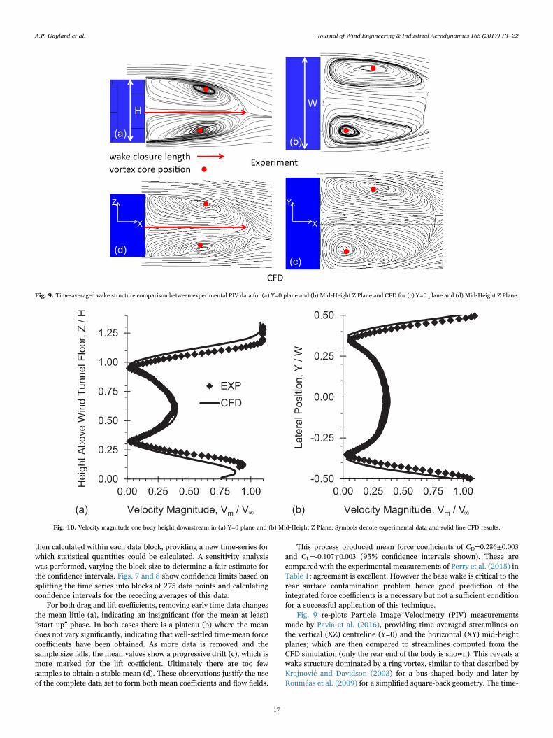
Fig. 9 re-plots Particle Image Velocimetry (PIV) measurementsmade by Pavia et al. (2016), providing time averaged streamlines onthe vertical (XZ) centreline (Y=0) and the horizontal (XY) mid-heightplanes; which are then compared to streamlines computed from theCFD simulation (only the rear end of the body is shown). This reveals awake structure dominated by a ring vortex, similar to that described byKrajnović and Davidson (2003) for a bus-shaped body and later byRouméas et al. (2009) for a simplified square-back geometry. The time-

Experiment

X

Z

X

Y

(b)

CFD

(c) (d)

(a)

wake closure lengthvortex core posi on

WH

Fig. 9. Time-averaged wake structure comparison between experimental PIV data for (a) Y=0 plane and (b) Mid-Height Z Plane and CFD for (c) Y=0 plane and (d) Mid-Height Z Plane.

0.00

0.25

0.50

0.75

1.00

1.25

0.00 0.25 0.50 0.75 1.00

EXPCFD

Hei

ghtA

bove

Win

dTu

nnel

Floo

r,Z

/H

Velocity Magnitude, Vm / V

Late

ralP

ositi

on,Y

/W

Velocity Magnitude, Vm / V

-0.50

-0.25

0.00

0.25

0.50

0.00 0.25 0.50 0.75 1.00

(a) (b)∞ ∞

Fig. 10. Velocity magnitude one body height downstream in (a) Y=0 plane and (b) Mid-Height Z Plane. Symbols denote experimental data and solid line CFD results.

A.P. Gaylard et al. Journal of Wind Engineering & Industrial Aerodynamics 165 (2017) 13–22

17

averaged wake structure is well-captured by the CFD simulation.Comparing Fig. 9(a) and (d) shows the vortex core position for thelower leg of the ring vortex sitting slightly too low in the CFDsimulation, due to reduced up-wash lower wake. In addition, the nearwake closure occurs slightly later in the simulated flow field, leading toa near wake 4.5% longer than that measured. In the horizontal plane(Fig. 9(b) and (c)), the overall topology is replicated, but the vortex corelocation provided by the CFD simulation compares less well toexperiment. This is likely a function of a lateral wake bi-stabilityidentified for this bluff body by Pavia et al. (2016) and the smaller time-sample obtainable in CFD (6 s) against experiment (137.7 s). Thus, it ispossible for the CFD simulation to be recovering the same time-dependant flow field as experiment, but have a different mean vortexring orientation because the run time is insufficient to capture thelateral switches in flow structure seen in the longer experiment.

Additional confirmation of the degree to which the CFD simulationsrecover physically realistic wake aerodynamics is provided by Fig. 10,

which shows the variation of velocity magnitude (relative to thefreestream velocity) at an X-location one body height (H) downstreamof the base. This location was selected as it corresponds to the positionof the vortex core. It is clear that the CFD simulation has captured thevelocity deficit in the central part of the wake. The largest differencesare seen in the y=0 plane (a) in regions of the wake affected by theupper free shear layer and the flow emerging from underneath themodel.

A final insight into the results of the aerodynamic simulation isprovided in Fig. 11. This plots the fraction of turbulent kinetic energyresolved in the wake (at the same downstream location) along with thedistribution of the absolute values of simulated and modelled turbulentkinetic energy. This shows that the level of spatial resolution used issufficient to resolve more than 80% of the energy through the bulk ofthe wake flow.

Hence, it is clear that the CFD simulation has replicated the wakestructure well and that the initial aerodynamics simulation provides a

-0.75

-0.50

-0.25

0.00

0.25

0.50

0.75

0 20 40 60 80

-0.75

-0.50

-0.25

0.00

0.25

0.50

0.75

0.7 0.8 0.9 1.0

0.00

0.25

0.50

0.75

1.00

1.25

0 20 40 60 80

TKE_sim

TKE_mod

0.00

0.25

0.50

0.75

1.00

1.25

0.7 0.8 0.9 1.0

H/Z,roolFlennuT

dniW

evobAthgieH

Fraction of Turbulent Kinetic Energy Resolved

Late

ralP

ositi

on,Y

/W

(a) (c)

H/Z,roolFlennuT

dniW

evobAthgieH

(b)La

tera

lPos

ition

,Y/W

(d)

Turbulent Kinetic Energy,TKE / m2s-2

Turbulent Kinetic Energy,TKE / m2s-2

Fraction of Turbulent Kinetic Energy Resolved

Fig. 11. The fraction of turbulent kinetic energy resolved on the voxel lattice along with simulated and modelled turbulence kinetic energy levels (a) & (b) Y=0 plane and (c) & (d) Mid-Height Z Plane.

A.P. Gaylard et al. Journal of Wind Engineering & Industrial Aerodynamics 165 (2017) 13–22

18

good starting point for the surface contamination calculation.

3.2. Surface contamination simulation

3.2.1. Distribution patternThe subsequent surface contamination simulation was run for

3.34 s of simulated time, requiring 1.01×105 CPU.hours of computa-tional effort. Time-dependant particle and surface film data were

averaged to allow for comparison with the time-averaged flow field.The predicted surface contamination distribution obtained is shown inFig. 12(a) where it is compared to the equivalent experimental result(b).

The first point to note here is that the experimental data is adistribution of intensity (I) resulting from the use of a UV fluorescingdye in the water spray, whereas the computational image is based onfilm thickness (h). Hence, although the two are related (as h∝I for thinfilms) any comparison is qualitative and limited to the form of thedistribution (to aid interpretation two broken lines have been added to

Fig. 12. Rear surface contamination pattern from (a) CFD and (b) Experiment (Kabanovs et al., 2016). Broken lines delineate subjectively assessed regions of high, medium and lowsurface contamination obtained in the experiment.

Fig. 13. Relative surface film thickness and static pressure coefficient for (a) verticalcentreline and (b) horizontal line through the contamination maximum the CFDsimulation shows a radially distributed deposition of material, with a maximum on thevehicle centre line, at around 25% of the base height.

Fig. 14. An isosurface of water volume ratio (7.5×10-8) coloured by mean particlediameter shown with streamlines on the Y=0 Plane.

Fig. 15. Rear surface film mass time history.

A.P. Gaylard et al. Journal of Wind Engineering & Industrial Aerodynamics 165 (2017) 13–22

19

indicate the boundaries of zones of low, medium and high contamina-tion seen in the experiment).

The corners of the base are largely free of contaminant. This broadlyaligns with the experimental data, particularly on the centre line where thebounds of the zones of high and moderate contamination match well.However, the experiment shows the maximum sitting lower on the baseand the overall distribution spread more laterally. The latter feature is likelydue to the combination of lateral wake instability seen for this geometry andlonger data acquisition period available experimentally. However, the resultis sufficiently credible to permit the use of the CFD to provide some insightsinto the processes involved.

3.2.2. Surface contamination and base pressureA relationship between the accumulation of material on the base

and the local static pressure has been asserted by Costelli (1984)following wind tunnel experiments on a small hatchback car. Heobserved that areas of high contamination were associated with regionsof higher base pressure. This is generally borne out by the CFDsimulation, as can be seen by plotting average film thickness againststatic pressure on the vertical centreline and a horizontal plane throughthe deposition maximum (Fig. 13).

For inboard regions, higher base pressure is strongly associatedwith higher levels of surface contamination. At the edges of the base theCFD model predicts some pressure recovery, which is not matched bycontaminant deposits. A consideration of the deposition mechanismsprovides some explanation for this.

3.2.3. Deposition mechanismsThe basic process of deposition is illustrated in Fig. 14. This plots

streamlines on the vertical centreline against an isosurface of effectivewater volume ratio (Volume of particles/volume of voxel=7.5×10-8) co-loured by mean particle diameter. This shows the spray being advecteddownstream (a), away from the body, until the reversed flow in thelower lateral leg of the ring vortex (b) draws a fraction of the particlesback towards the vehicle. The bulk of the captured particles are held inthe lower part of the wake, with relatively little mixing into the upperpart of the ring vortex (c). It also appears that as the contaminantapproaches the rear surface it is drawn downwards by the local flowturning to align with the surface. It is notable that only a small fractionof the particles released into the flow (less than 1.0% by mass) aredeposited on the rear surface.

The retention of the largest fraction of particles in the lower part ofthe wake explains the position of the contamination maximum on therear surface. Its association with the return flow and subsequent rearstagnation point explains the relationship with regions of high basepressure suggested by Costelli (1984) and seen in Fig. 13. The deviationnoted from this association approaching the lower trailing edgeappears to be caused by local downwash in the flow field. Those seenapproaching the upper and body side edges are caused by the relativelack of contaminant in proximity to the rear surface in these areas.

The simulation also suggests that the main transport mechanism ofcontaminant to the rear surface is the flow reversal associated with thelower part of the ring vortex. Few particles appear to penetrate thelower shear layer. In addition, the distribution of mean particlediameter over the isosurface indicates that the process of turning theparticles leads to break-up, as the fraction of large particles decreasesas they approach the rear surface.

3.2.4. Rate of accumulationThe final set of observations provided in this work relate to the rate

of accumulation of material on the rear surface. The time histories offilm mass and its rate of deposition are provided in Figs. 15 and 16,respectively.

From Fig. 15 it is clear that over the period simulated, the filmaccumulates linearly, with 5.65 ×10 kg-5 of the dispersed phase depos-ited on the rear surface over the course of the simulation. The lineartrend aligns with simulations conducted for a fully-detailed roadvehicle by Jilesen et al. (2013), suggesting that the insights providedby this simple system are relevant to actual vehicles.

The reason for the linear accumulation of mass on the rear surfaceis provided in Fig. 16. This plots the time-history of the progressiveaverage (i.e. the start of the averaging window remains fixed, with newdata added sequentially) of the deposition rate (solid line), along withthe bounds for a 95% confidence interval (broken lines). As can beseen, the rate of deposition reaches a well-settled mean value after onesecond of simulated time. From then on the average rate remainslargely constant, reaching a final value of (1.7 ± 0.2) ×10 kg/s-5 ; only1.0% of the rate input into the simulation.

Fig. 16. Development of the average rate of rear film deposition.

Fig. 17. Relative film thickness profiles for 1≤t(s)≤3.24 on the (a) vertical centreline and

(b) a horizontal line through the surface contamination maximum.

A.P. Gaylard et al. Journal of Wind Engineering & Industrial Aerodynamics 165 (2017) 13–22

20

These observations indicate that although longer simulations willgenerate a thicker film (up to the point where the surface cannotsupport the liquid against gravity and aerodynamic shear, leading tofilm run-off) the form of the distribution is likely to remain unchanged.This view is confirmed by the time-series of relative film thicknessprofiles (i.e. film height divided by the maximum value along theprofile) presented in Fig. 17. These show relative film thicknessdistribution on the (a) vertical centreline and (b) a horizontal planethrough the contamination maximum. The individual profiles aresimilar over the time period shown, with differences diminishing asthe simulation progresses. This provides good evidence that althoughfilm thickness increases over time, the relative distribution does not.Hence, comparisons of relative distributions between relatively shortCFD calculations and longer experiments may be warranted.

4. Conclusions

An extended LB solver has been shown to provide an excellentrepresentation of the aerodynamics of a simple square-backed bluffbody, leading to a credible prediction of the relative distribution ofcontaminant on the rear surface. Thus the potential of this eddy-resolving method to predict these important characteristics is demon-strated.

Deposition of surface contaminant on the rear surface of arepresentative bluff body has been shown to be the result of sprayentrainment by the lower part of the wake ring vortex. Relatively littlematerial appears to be advected across the lower shear layer.

Surface contaminant accumulates preferentially in regions of higherbase pressure, as suggested by Costelli (1984). Exceptions to this trendare seen (a) close to the lower edge of the base, due to local wakedownwash and (b) close to the remaining edges, due to low localavailability of contaminant.

In this simulation, the fraction of emitted material deposited on therear surface was small, only 1.0% of the total mass of contaminantintroduced into the domain.

In common with actual vehicles, the accumulation of contaminantis linear, with the deposition rate and relative distribution changinglittle over time. This suggests that shorter CFD simulations can becompared to longer experiments. It also suggests that the rate ofaccumulation is a useful metric for future studies, as is constant andusefully related to vehicle development objectives: i.e. vehicles oper-ated in the environment will always accumulate contaminant, butreducing the rate at which this occurs can help differentiate betweendesigns.

Finally, for real vehicles, the source of surface contamination isspray generated by tyres lifting water containing solid contaminantsfrom wet road surfaces. Also, the wheels generate their own wakestructure. These elements have been omitted from this study, so thenext stage in the systematic application of simplified vehicle geometriesto this problem should be based around a standard body whichincorporates wheels.

Acknowledgements

The authors would like to thank Giancarlo Pavia (LoughboroughUniversity) for re-plotting PIV data from Pavia et al. (2016) to facilitatedirect comparison with the CFD simulation presented here, and DrAnna-Kristina Perry (Loughborough University) for providing theadditional experimental data used in Fig. 10.

The work of A. P. Gaylard and A. Kabanovs is supported by JaguarL and Rover and the UK-EPSRC grant EP/K014102/1 as part of thejointly funded Programme for Simulation Innovation.

D. A. Lockerby's time has been financially supported by EPSRCgrants EP/N016602/1, EP/K038664/1 and EP/I011927/1.

References

Ahmadi, G., Li, A., 2000. Computer simulation of particle transport and deposition near asmall isolated building. J. Wind Eng. Ind. Aerodyn. 84 (1), 23–46. http://dx.doi.org/10.1016/S0167-6105(99)00048-3.

Carr, G. W., Stapleford, W. R. (1983). Blockage Effects in Automotive Wind-TunnelTesting. SAE Technical Paper 860093. In: Proceedings of the SAE InternationalCongress and Exposition, February 24 – 28, 1986, Detroit, MI, USA. Warrendale:Society of Automotive Engineers, Inc. DOI:10.4271/860093.

Chen, H., Chen, S., Matthaeus, W.H., 1992. Recovery of the Navier-Stokes equationsusing a lattice-gas Boltzmann method. Phys. Rev. A 45 (8), R5339–R5342. http://dx.doi.org/10.1103/PhysRevA.45.R5339.

Chen, H., Teixeira, C., Molvig, K., 1997. Digital physics approach to computational fluiddynamics: some basic theoretical features. Int. J. Mod. Phys. C 8 (4), 675–684.http://dx.doi.org/10.1142/S0129183197000576.

Chen, H., Kandasamy, S., Orszag, S., Shock, R., et al., 2003. Extended Boltzmann kineticequation for turbulent flows. Science 301 (5633), 633–636. http://dx.doi.org/10.1126/science.1085048.

Costelli, A. F. (1984). Aerodynamic Characteristics of the Fiat UNO Car. SAE TechnicalPaper 840297. In: Proceedings of the SAE 1984 International Congress &Exposition, Detroit, February 27–March 2 1984. Warrendale: SAE International.doi: 10.4271/840297.

Fares, E., 2006. Unsteady flow simulation of the Ahmed reference body using a latticeBoltzmann approach. Comput. Fluids 35 (8–9), 40–95. http://dx.doi.org/10.1016/j.compfluid.2005.04.011.

Fischer, O., Kuthada, T., Mercker, E., Wiedemann, J. et al., (2010). CFD Approach toEvaluate Wind-Tunnel and Model Setup Effects on Aerodynamic Drag and Lift forDetailed Vehicles. SAE Technical Paper 2010-01-0760. In: Proceedings of the SAE2010 World Congress, April 13–15,Detroit, MI, USA. Warrendale: SAEInternational. DOI:10.4271/2010-01-0760.

Fischer, O., Kuthada, T., Wiedemann, J., Dethioux, P. et al. (2008). CFD Validation Studyfor a Sedan Scale Model in an Open Jet Wind Tunnel. SAE Technical Paper 2008-01-0325. In: Proceedings of the SAE 2010 World Congress, April 14–17,Detroit, MI,USA. Warrendale: SAE International. DOI:10.4271/2008-01-0325.

Gaylard, A., Pitman, J., Jilesen, J., Gagliardi, A., et al., 2014. Insights into Rear SurfaceContamination Using Simulation of Road Spray and Aerodynamics. SAE Int. J.Passeng. Cars - Mech. Syst. 7 (2), 673–681. http://dx.doi.org/10.4271/2014-01-0610.

Hangan, H., 1999. Wind-driven rain studies. A C-FD-E approach. J. Wind Eng. Ind.Aerodyn. 81 (1–3), 323–331. http://dx.doi.org/10.1016/S0167-6105(99)00027-6.

Howell, J., Passmore, M., Tuplin, S., 2013. Aerodynamic drag reduction on a simple car-like shape with rear upper body taper. SAE Int. J. Passeng. Cars - Mech. Syst. 6 (1),52–60. http://dx.doi.org/10.4271/2013-01-0462.

Howell, J., Sheppard, A., Blakemore, A. (2003). Aerodynamic Drag Reduction for aSimple Bluff Body Using Base Bleed. SAE Technical Paper 2003-01-0995.In: Proceedings of the SAE 2003 World Congress, March 3–6,Detroit, MI, USA.Warrendale: SAE International. DOI:10.4271/2003-01-0995.

Howell, J., Le Good, G., (2008). The Effect of Backlight Aspect Ratio on Vortex and BaseDrag for a Simple Car-Like Shape. SAE Technical Paper 2008-01-0737. In:Proceedings of the SAE 2008 World Congress, April 14–17,Detroit, MI, USA.Warrendale: SAE International. DOI:10.4271/2008-01-0737.

Hu, X., Liao, L., Lei, Y., Yang, H., et al., 2015. A numerical simulation of wheel spray forsimplified vehicle model based on discrete phase method. Adv. Mech. Eng. 7 (7), 1–8. http://dx.doi.org/10.1177/1687814015597190.

Jilesen, J., Alajbegovic, A., Duncan, B., 2015. Soiling and Rain Simulation for GroundTransportation. In: Proceedings of the 7th European-Japanese Two-Phase FlowGroup Meeting (7TH-EUJPTPFGM 2015), 11-15 October 2015, Zermatt,Switzerland.

Jilesen, J., Gaylard, A., Duncan, B., Konstantinov, A., et al., 2013. Simulation of rear andbody side vehicle soiling by road sprays using transient particle tracking. SAE Int. J.Passeng. Cars - Mech. Syst. 6 (1), 424–435. http://dx.doi.org/10.4271/2013-01-1256.

Johl, G., Passmore, M., Render, P., 2004. Design methodology and performance of anindraft wind tunnel. Aeronaut. J. 108 (1087), 465–473.

Kabanovs, A., Varney, M., Garmory, A., Passmore, M. et al. (2016). Experimental andComputational Study of Vehicle Soiling on a Generic Hatchback Body. SAE TechnicalPaper 2016-01-1604. In: Proceedings of the SAE 2016 World Congress andExhibition, April 12–14, Detroit, MI, USA. Warrendale: SAE International. DOI:10.4271/2016-01-1604.

Krajnović, S., Davidson, L., 2003. Numerical study of the flow around a bus-shaped body.J. Fluids Eng. 125 (3), 500–509. http://dx.doi.org/10.1115/1.1567305.

Krastev, V., Bella, G. (2011). On the Steady and Unsteady Turbulence Modeling inGround Vehicle Aerodynamic Design and Optimization. SAE Technical Paper 2011-24-0163. In: Proceedings of the ICE2011 - 10th International Conference onEngines & Vehicles, September 11–15, 2011, Capri, Napoli, Italy. Warrendale: SAEInternational. DOI:10.4271/2011-24-0163.

Kuthada, T., Cyr, S., 2006. Approaches to vehicle soiling. In: Wiedermann, J., Hucho,W.H. (Eds.), Progress in Vehicle Aerodynamics, IV, Numerical methods. Expert-Verlag, Renningen, 111–123.

Lajos, T., Preszler, L., Finta, L., 1986. Effect of moving ground simulation on the flowpast bus models. J. Wind Eng. Ind. Aerodyn. 22 (2), 271–277. http://dx.doi.org/10.1016/0167-6105(86)90090-5.

Le Good, G., Garry, K., (2004). On the Use of Reference Models in AutomotiveAerodynamics. SAE Technical Paper 2004-01-1308. In: Proceedings of the SAE 2004World Congress, March 8–11, 2004, Detroit, MI, USA. Warrendale: SAE

A.P. Gaylard et al. Journal of Wind Engineering & Industrial Aerodynamics 165 (2017) 13–22

21

International. DOI:10.4271/2004-01-1308.Lietz, R., Mallick, S., Kandasamy, S., Chen, H (2002). Exterior Airflow Simulations Using

a Lattice Boltzmann Approach. SAE Technical Paper 2002-01-0596. In: Proceedingsof the SAE 2002 World Congress, March 4–7, 2002, Detroit, MI, USA. Warrendale:SAE International. DOI:10.4271/2002-01-0596.

Littlewood, R., Passmore, M., Wood, D., 2011. An investigation into the wake structure ofsquare back vehicles and the Effect of structure modification on resultant vehicleforces. SAE Int. J. Engines 4 (2), 2629–2637. http://dx.doi.org/10.4271/2011-37-0015.

Littlewood, R., Passmore, M. (2010). The Optimization of Roof Trailing Edge Geometryof a Simple Square-Back. SAE Technical Paper 2010-01-0510, In: Proceedings of theSAE 2010 World Congress, April 13–15, 2010, Detroit, MI, USA. Warrendale: SAEInternational. DOI:10.4271/2010-01-0510.

Mamou, M., Cooper, K.R., Benmeddour, A., Khalid, M., et al., 2008b. Correlation of CFDpredictions and wind tunnel measurements of mean and unsteady wind loads on alarge optical telescope. J. Wind Eng. Ind. Aerodyn. 96 (6–7), 793–806. http://dx.doi.org/10.1016/j.jweia.2007.06.050.

Mamou, M., Tahi, A., Benmeddour, A., Cooper, K.R., Abdallah, I., et al., 2008a.Computational fluid dynamics simulations and wind tunnel measurements ofunsteady wind loads on a scaled model of a very large optical telescope: acomparative study. J. Wind Eng. Ind. Aerodyn. 96 (2), 257–288. http://dx.doi.org/10.1016/j.jweia.2007.06.002.

Maycock, G. (1966). The problem of water thrown up by vehicles on wet roads.Harmondsworth: Road Research Laboratory. (LR4).

Meroney, R.N., 2006. CFD prediction of cooling tower drift. J. Wind Eng. Ind. Aerodyn.94 (6), 463–490. http://dx.doi.org/10.1016/j.jweia.2006.01.015.

Mundo, C., Sommerfeld, M., Tropea, C., 1995. Droplet-wall collisions: experimentalstudies of the deformation and breakup process. Int. J. Multiph. Flow. 21 (2),151–173. http://dx.doi.org/10.1016/0301-9322(94)00069-V.

O'Rourke, P., Amsden, A. (1987). The TAB Method for Numerical Calculation of SprayDroplet Breakup. SAE Technical Paper 872089. In: Proceedings of the InternationalFuels and Lubricants Meeting and Exposition, Toronto, Ontario, November 2–5,1987. Warrendale: The Society of Automotive Engineers, Inc. DOI:10.4271/872089.

O'Rourke, P., Amsden, A. (2000). A Spray/Wall Interaction Submodel for the KIVA-3Wall Film Model. SAE Technical Paper 2000-01-0271. In: Proceedings of the SAE2000 World Congress, March 6–9, 2000, Detroit, MI, USA. Warrendale: SAEInternational. DOI:10.4271/2000-01-0271.

O'Rourke, P., Amsden, A. (1996). A Particle Numerical Model for Wall Film Dynamics inPort-Injected Engines. SAE Technical Paper 961961. In: Proceedings of theInternational Fall Fuels & Lubricants Meeting & Exposition, San Antonio, Texas,October 14–17, 1996. Warrendale: Society of Automotive Engineers, Inc.DOI:10.

4271/961961.Paschkewitz, J. S. (2006). A comparison of dispersion calculations in bluff body wakes

using LES and unsteady RANS. United States: Lawrence Livermore NationalLaboratory. (UCRL-TR-218576). ) ⟨https://e-reports-ext.llnl.gov/pdf/329543.pdf⟩.

Pavia, G., Passmore, M., Gaylard, A. (2016). Influence of Short Rear End Tapers on theUnsteady Base Pressure of a Simplified Ground Vehicle. SAE Technical Paper 2016-01-1590. In: Proceedings of the SAE 2016 World Congress and Exhibition, April 12–14, Detroit, MI, USA. Warrendale: SAE International. DOI: 10.4271/2016-01-1590.

Paz, C., Suárez, E., Gil, C., Concheiro, M., 2015. Numerical study of the impact ofwindblown sand particles on a high-speed train. J. Wind Eng. Ind. Aerodyn. 145,87–93. http://dx.doi.org/10.1016/j.jweia.2015.06.008.

Perry, A., Passmore, M., Finney, A., 2015. Influence of short rear end tapers on the basepressure of a simplified vehicle. SAE Int. J. Passeng. Cars - Mech. Syst. 8 (1),317–327. http://dx.doi.org/10.4271/2015-01-1560.

Persoon, J., van Hooff, T., Blocken, B., Carmeliet, J., et al., 2008. On the impact of roofgeometry on rain shelter in football stadia. J. Wind Eng. Ind. Aerodyn. 96 (8–9),1274–1293. http://dx.doi.org/10.1016/j.jweia.2008.02.036.

Pope, S.B., 2013. Turbulent Flows. Cambridge University Press, Cambridge, UK.Rouméas, M., Gilliéron, P., Kourta, A., 2009. Analysis and control of the near-wake flow

over a square-back geometry. Comput. Fluids 38 (1), 60–70. http://dx.doi.org/10.1016/j.compfluid.2008.01.009.

Samples M., Gaylard A.P., Windsor S., 2010. The aerodynamic development of the RangeRover Evoque. In: Proceedings of the 8th MIRA International Conference on VehicleAerodynamics, 13-14 October 2010, Grove, Oxfordshire. Nuneaton: MIRA Ltd, pp.380–388.

Sims-Williams, D., Duncan, B. (2003). The Ahmed Model Unsteady Wake: Experimentaland Computational Analyses. SAE Technical Paper 2003-01-1315. In: Proceedings ofthe SAE 2003 World Congress, March 3–6, Detroit, MI, USA. Warrendale: SAEInternational. DOI: 10.4271/2003-01-1315.

Syms, G.F., 2008. Simulation of simplified-frigate airwakes using a lattice-Boltzmannmethod. J. Wind Eng. Ind. Aerodyn. 96 (6–7), 1197–1206. http://dx.doi.org/10.1016/j.jweia.2007.06.040.

Volpe, R., Ferrand, V., Da Silva, A., Le Moyne, L., 2014. Forces and flow structuresevolution on a car body in a sudden crosswind. J. Wind Eng. Ind. Aerodyn. 128,114–125. http://dx.doi.org/10.1016/j.jweia.2014.03.006.

Xu, Z.G., Walklate, P.J., Rigby, S.G., Richardson, G.M., 1998. Stochastic modelling ofturbulent spray dispersion in the near-field of orchard sprayers. J. Wind Eng. Ind.Aerodyn. 74–76, 295–304. http://dx.doi.org/10.1016/S0167-6105(98)00026-9.

Yang, W.B., Zhang, H.Q., Chan, C.K., Lin, W.Y., 2004. Large eddy simulation of mixinglayer. J. Comput. Appl. Math. 163 (1), 311–318. http://dx.doi.org/10.1016/j.cam.2003.08.076.

A.P. Gaylard et al. Journal of Wind Engineering & Industrial Aerodynamics 165 (2017) 13–22

22