simulation of stick-slip friction
TRANSCRIPT
DEPARTMENT OF Mechanics and Maritime Sciences
CHALMERS UNIVERSITY OF TECHNOLOGY Gothenburg, Sweden 2020
www.chalmers.se
Simulation of stick-slip friction Nonlinear modelling and experimental validation Master’s thesis in Applied Mechanics
Arian Nasseri Vince Heszler

MASTER’S THESIS IN APPLIED MECHANICS
Simulation of stick-slip friction
Nonlinear modelling and experimental Validation
Arian Nasseri
Vince Heszler
Department of Mechanics and Maritime Sciences
Division of Dynamics
CHALMERS UNIVERSITY OF TECHNOLOGY
Göteborg, Sweden 2020
Simulation of stick-slip friction
Nonlinear modelling and experimental Validation
Arian Nasseri, Vince Heszler
© Arian Nasseri, Vince Heszler, 2020-06-10
Master’s Thesis 2020:31
Department of Mechanics and Maritime Sciences
Division of Dynamics
Chalmers University of Technology
SE-412 96 Göteborg
Sweden
Telephone: + 46 (0)31-772 1000
Cover:
CAE model made from stick-slip Ziegler ssp-04 test bench.
Department of Mechanics and Maritime Sciences
Göteborg, Sweden 2020-06-10
I
Simulation of stick-slip friction
Nonlinear modelling and experimental Validation
Arian Nasseri, Vince Heszler
Department of Mechanics and Maritime Sciences
Division of Dynamics
Chalmers University of Technology
Abstract
A determining factor of the quality of a vehicle is the audible interior squeak and rattle (S&R) noise. This study aimed to model the friction induced stick-slip phenomenon, which is the main cause behind the squeak noise. This was done by first doing tests on a stick-slip test bench. The results gained from the experiments were processed and used for the FE model. Secondly a FE model was set up, on which a parametric investigation was done. During FE modeling an experiment postprocessing method was established and validated. Many FE cases were run, and the results were compared to the experimental ones. For the comparisons some metrics were established which can be related to the severity of the stick-slip event. The main achievement of this work was the model setup approach and the validated FE model which form the basis of the simulation and follow the experimental trends of the stick-slip phenomenon. With the help of this study engineers will be able to simulate stick-slip events in CAE environment and determine its severity early and upfront in the product development process.
Key words: Stick-slip events – Nonlinear friction modelling – Contact modelling –
Squeak and rattle – Abaqus
II
Contents
Abstract ............................................................................................................................................... I
Preface ................................................................................................................................................. V
Notations ......................................................................................................................................... VII
1 Introduction ................................................................................................................................. 1
1.1 Background .......................................................................................................................... 1
1.2 Physical setup ..................................................................................................................... 1
1.3 Limitations ........................................................................................................................... 2
1.4 Outline .................................................................................................................................... 3
2 Methodology ................................................................................................................................ 4
3 Theory ............................................................................................................................................ 5
3.1 Contact Formulation ........................................................................................................ 5
3.1.1 Gap\Penetration detection approaches ......................................................... 6
3.1.2 Contact tracking approach ................................................................................... 7
3.1.3 Sticking constitutive equation ............................................................................ 7
3.1.4 Coulomb Friction ...................................................................................................... 7
3.1.5 Elastic Slip ................................................................................................................... 8
3.1.6 Lagrange multiplier method or penalty method for contact -constraint? .................................................................................................................................... 8
3.1.7 Rough ............................................................................................................................. 9
3.2 Damping ................................................................................................................................ 9
3.2.1 Material Damping ..................................................................................................... 9
3.2.2 Numerical Damping.............................................................................................. 10
3.2.3 Contact Damping ................................................................................................... 10
3.3 Dynamic Substructuring ............................................................................................. 11
4 Physical Tests ........................................................................................................................... 13
4.1 Experimental setup: The Ziegler ssp-04 .............................................................. 13
4.2 Experiment’s Outputs ................................................................................................... 15
4.2.1 Coefficients of Static and Dynamic Friction. .............................................. 15
4.3 Modal Analysis ................................................................................................................. 16
4.4 Test Setups with friction ............................................................................................. 19
4.4.1 Constant Force ........................................................................................................ 20
4.4.2 Constant Velocity ................................................................................................... 23
5 FEM Implementation ............................................................................................................ 25
III
5.1 Abaqus ................................................................................................................................. 25
5.2 Elements ............................................................................................................................. 25
5.3 Boundary Conditions .................................................................................................... 26
5.4 Coefficients of friction .................................................................................................. 26
5.5 Decay coefficient ............................................................................................................. 29
5.6 Material Damping ........................................................................................................... 31
5.7 Dynamic Substructure .................................................................................................. 34
6 Parametric Investigation ..................................................................................................... 35
6.1 Number of step study ................................................................................................... 35
6.2 Mesh Size Study............................................................................................................... 36
6.3 Damping Study ................................................................................................................ 38
6.3.1 Material Damping .................................................................................................. 38
6.4 Numerical Damping ...................................................................................................... 42
6.4.1 Contact Damping ................................................................................................... 43
6.5 Decay coefficient ............................................................................................................. 45
6.6 Elastic slip .......................................................................................................................... 47
6.7 Friction Coefficient ........................................................................................................ 48
6.7.1 Static Friction Coefficient ................................................................................... 48
6.7.2 Dynamic Friction coefficient ............................................................................ 50
6.8 Full Model vs. Super-Element ................................................................................... 52
7 Results and discussions ....................................................................................................... 55
7.1 Postprocessing of Output Signals ............................................................................ 55
7.1.1 Selecting Signal Parts ........................................................................................... 55
7.1.2 Metrics compared ................................................................................................. 56
7.2 Material Pair ..................................................................................................................... 57
8 Conclusion ................................................................................................................................. 61
8.1 Future work ...................................................................................................................... 61

IV
V
Preface
In this study, stick-slip phenomenon had been investigated via experiments on a
testbench as well as via simulations. The work was carried out from January 2020 to
June 2020. The thesis is a part of an industrial PhD work carried out at Volvo Car
Corporation, Solidity Department, Göteborg, Sweden. The project is financed through
Volvo Car Corporation.
This part of the project has been carried out with Mohsen Bayani as an industrial
supervisor and Thomas Abrahamsson as examiner. All test have been carried out in the
laboratory of Volvo Car Corporation. Our co-workers Anneli Rosell, Mohsen Bayani
and Tommy Johansson are highly appreciated for their help with setting up and
planning the tests. We would also like to thank Thomas Abrahamsson for supervising
and guiding us.
Finally, it should be noted that the tests could never have been conducted without the
sense of high quality and professionalism of the laboratory staff.
Göteborg June 2020-06-10
Arian Nasseri, Vince Heszler

VI
VII
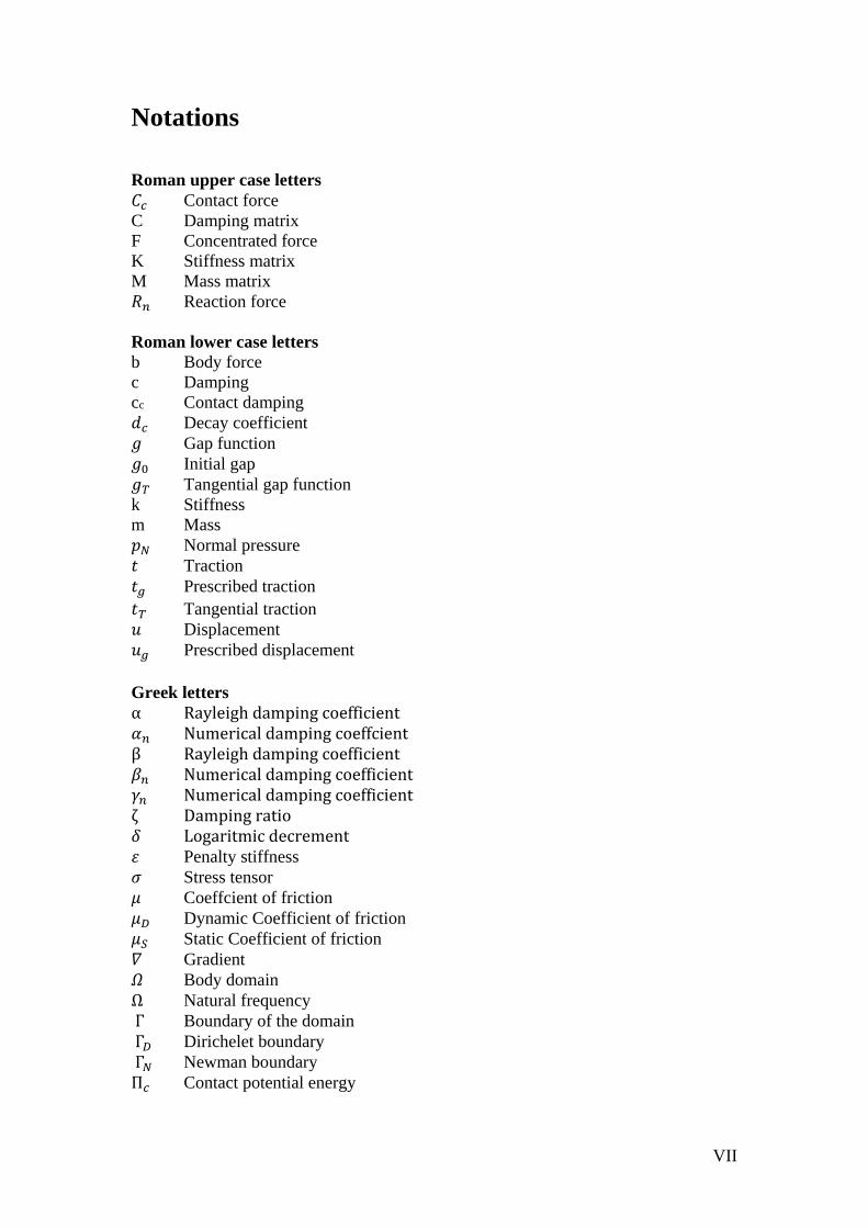
Notations
Roman upper case letters
𝐶𝑐 Contact force
C Damping matrix
F Concentrated force
K Stiffness matrix
M Mass matrix
𝑅𝑛 Reaction force
Roman lower case letters
b Body force
c Damping
cc Contact damping
𝑑𝑐 Decay coefficient
𝑔 Gap function
𝑔0 Initial gap
𝑔𝑇 Tangential gap function
k Stiffness
m Mass
𝑝𝑁 Normal pressure
𝑡 Traction
𝑡𝑔 Prescribed traction
𝑡𝑇 Tangential traction
𝑢 Displacement
𝑢𝑔 Prescribed displacement
Greek letters
α Rayleigh damping coefficient 𝛼𝑛 Numerical damping coeffcient β Rayleigh damping coefficient 𝛽𝑛 Numerical damping coefficient 𝛾𝑛 Numerical damping coefficient ζ Damping ratio 𝛿 Logaritmic decrement 휀 Penalty stiffness
𝜎 Stress tensor
𝜇 Coeffcient of friction
𝜇𝐷 Dynamic Coefficient of friction
𝜇𝑆 Static Coefficient of friction
𝛻 Gradient
𝛺 Body domain
Ω Natural frequency
Γ Boundary of the domain
Γ𝐷 Dirichelet boundary
Γ𝑁 Newman boundary
Π𝑐 Contact potential energy
VIII
Abbreviations
AL Aluminum
CAE Computer Aided Engineering CMS Component Mode Synthethis
DoF Degree of Freedom
FE Finite Element FEA Finite Element Analysis FEM Finite Element Method FFT Fast Fourier Transform MPC Multi-Point Constraint PCABS Polycarbonate/Acrylonitrile Butadiene Styrene PP Polypropylene
RPN Risk Priority Number S&R Squeak & Rattle (noises) VCC Volvo Car Corporation


CHALMERS, Mechanics and Maritime Sciences, Master’s Thesis 2020:31 1
1 Introduction
The Solidity department at Volvo Car Corporation (VCC) is concerned with the undesired squeak & rattle (S&R) noises, which occur when adjacent parts are sliding and/or impacting on each other. Too high S&R noises contribute to poor user experience and might give the impression of low quality. The Solidity department is working on pushing engineering activities to early phases of product development. A major challenge for the group is to improve S&R verification at early phases, to attain shorter lead times and less need for expensive and time consuming physical tests. There is a need to improve the CAE methods used today to secure an upfront robust verification regarding S&R noises. Stick-slip is a friction induced nonlinear phenomenon, which contributes to the squeaking noise. This thesis work focuses on the CAE modelling of stick-slip events and aims to give guidelines for engineers at VCC to establish a better model sutups in CAE environment.
1.1 Background
In order to be able to predict S&R noises upfront in a robust way, VCC has invested heavily in research. The E-LINE , which is currently used at VCC, and is a method for predicting squeak and rattle events in linear domain [1, 2]. However, this method does not model the friction event, thus not giving sufficient information on the event itself, and the severity of the noise it generates. This thesis supports a doctoral work. The aim is to predicting S&R noises with the help of Finite Element Analysis (FEA). This part of the work is to build an accurate enough FE model, which can capture the stick-slip events, and to investigate how Finite Element (FE) settings influence the outcome. Furthermore, to create an assessment method for correlating and comparing the fundamental parameters, which contribute to the annoyance level, between simulation and experiments. This work is a continuation of a started, but not finished project, where the FE geometry model was done. It is also very similar to a previous thesis work [1] , where the aim and goal were similar, but it targeted rattle instead of stick-slip events. Similarly to the previous thesis work, the main aim was to to find a model setup approach and the criteria to verify the method which was taken from squeak severity metric, based on the Risk Priority Number (RPN). The RPN describes the severity of stick-slip events, which can be correlated to noise. The RPN number consist of parameters gained from the acceleration and force signals from the measurement [3]. The main goal of this thesis was to find correlation between these parameters in FEA and measurements.
1.2 Physical setup
In this section the physical setup, and the principles of how the experimental machine works is described on the FE model, since it is easier to understand it, and has a clearer picture.
2 CHALMERS, Mechanics and Maritime Sciences, Master’s Thesis 2020:31
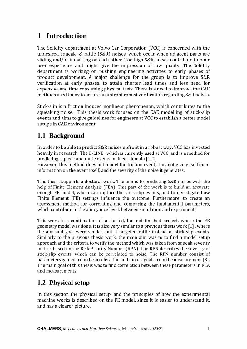
Figure 1-1 Finite Element model of the experimental setup, with description
The model consists of two objects: the carriage, which moves with a constant predefined speed in the z direction. All the other pars are connected to each other. The base fixture can move free in the y direction, however there is a force givn from the infeed unit pushing the vertical fixture so the sample carrier and the carriage is in contact. The friction is happening between the carriage and the sample carrier. The spring stores energy while the sample carrier moves in z direction. Due to this spring the stick-slip phenomenon happening. The FE model and the experimental setup is described more in detail in section 4.1 and 5.
1.3 Limitations
When it comes to create a CAE model of an experimental setup, one always have to make assumpions, as well as to set up acceptance bounds for the precision of the model. There can always be a more detailed CAE model, but maybe it would not give much better results, while it would come with adittional cost. During the thesis many of these decisions had to be made. Not all of the experimental setups dimensions were given. Dimensions had to be measured from drawings of the setup or measured by hand with the help of a caliper. Since the experimental setup was calibrated, there was no possibility to take it apart to measure parts correctly. Some dimensions were unaccessible, therefore those were estimated with the help of pictures. Overall the important dimensions were captured with good precision. One very important parameter from the experiment would have been the displacement of the sample carrier. However it could not be measured. Even
CHALMERS, Mechanics and Maritime Sciences, Master’s Thesis 2020:31 3
though there was a displacement sensor measuring the displacement of the spring plate. An instrument only gave the reset force, or the friction force, of the system. Calculating displacement from the accelerometer provided to be too difficult, and would have taken too much time, since every signal would have needed special treatment. The softwares available were the same used at VCC. ANSA 19.1.0 and 18.1.4 was used for preprocessing. The solver used was ABAQUS 2017, while META 18.1.1 for postprocessing together with MATLAB R2017b. Finally, the biggest limitation, as usually, was time. The COVID-19 pandemic just made it more difficult, since VCC was only operating three days a week from April. Also the most of the time home office was in practice. However, most of the problems were solved, and good correlation was achieved.
1.4 Outline
The outline of this thesis work describes the layout and content of the project. Chapter 2 provides a brief discussion of the methodology that is used to obtain the results of this thesis. In Chapter 3, formulations of contact, friction, various types of damping, and substructuring method were discussed. Chapter 4 firstly, presents the test bench, and then it provides information about output parameters and how they behave by changing the inputs. Chapter 5 contains the implementation of the CAE model and the method that is used for defining a friction model in the system. Chapter 6 contains investigations of the effect of critical parameters on the system output and correlation of the CAE results with the experimental results. Chapter 7 provides information on a post-processing procedure and studies the trend of the CAE model in various test cases in comparison to the experimental test and discusses the limitations of the CAE model.
4 CHALMERS, Mechanics and Maritime Sciences, Master’s Thesis 2020:31
2 Methodology
This thesis aimed to build and validate a FE model of the experimental setup, and to correlate those. The whole method can be divided into three major parts. In the first part the task was to set up and validate a model, which can capture the system responses by just changing the fundamental friction parameters, which should come from the experiments. In order to validate the model, a frequency analysis was performed on the experimental setup, without having contact, and therefore less nonlinearities in the system. The results were compared to a modal FEA also without contact. Comparing the eigenfrequencies helped to calibrate and validate the stiffness and mass properties of the system, which are the most important factors in the FEA. Also, from the acceleration-time and force-time signals, with the help of the logarithmic decrement, the damping of the system was estimated. The second part was about model correlation. Time domain implicit analysis including friction were compared to measurements. During this step the FEA parametes and solver settings were tested and calibrated. This was done by two different experiment cases. The crucial friction parameters, which were changed during the batch run in step three, were calculated through an assessment method, which used the outputs from the experiments as an. The method was based on papers [4], and from the experimental instruments manual [3]. When the method gave very close input parameters for FE to the ones which produced good correlation with the experimental results, the model was assumed valid. The third and final part batch cases on different contact material pairs and experiment cases were run. The FEA results were compared with the experimental ones. Finally the results were interpreted and discussed. Guidelines were set up for how to model friction and stick-slip. Possible future work and continuation guidelines were also set up.
CHALMERS, Mechanics and Maritime Sciences, Master’s Thesis 2020:31 5
3 Theory
3.1 Contact Formulation
To drive the contact formulation normal to the surfaces, the strong format of the equilibrium condition is given by [5]
𝜎 ⋅ 𝛻 = 𝑏 in 𝛺 3-1
Where 𝜎 ⋅ 𝛻 is the scalar product of the stress tensor (𝜎) and gradient (𝛻), 𝑏 is the body force, and 𝛺 is the body domain. The boundary conditions can be defined as bellow
𝑢 = 𝑢𝑔 𝑜𝑛 Γ𝐷 3-2
𝜎 ⋅ 𝑛 = 𝑡 = 𝑡𝑔 𝑜𝑛 Γ𝑁 3-3
where 𝑢 is displacement, 𝑢𝑔 the prescribed, 𝑛 is the normal vector of the
boundary surface, 𝑡 is the traction or stress vector with 𝑡𝑔 it’s prescribed
amount, Γ𝐷 is the Dirichelet boundary, Γ𝑁 is the Newmann boundary (𝜕Ω = Γ𝑁 ∪ Γ𝐷). If we define the gap function as
𝑔 = 𝑔0 − 𝑢𝑛 ≥ 0 3-4
Where 𝑢𝑛 is the scalar product of displacement and normal vector that, is normal to the gap surface. Based on the Kuhn – Tucker condition two surfaces are not in contact when the gap is larger than zero and therefore the reaction force is then zero. In case of contact, the gap between two surfaces is zero while the reaction force on a surface is positive and acting in the opposite direction of the surface normal vector. We then have
𝑅𝑛 ≤ 0 3-5
𝑔 ∙ 𝑅𝑛 = 0 3-6
Where 𝑅𝑛 is the reaction force. The weak format of the equilibrium equation can be written as
∫ 𝜎 ∶ (𝛿𝑢 ⨂∇) 𝑑Ω − ∫ 𝑏 ∙
ΩΩ
𝛿𝑢 𝑑Ω − ∫ 𝑡 ∙ Γ
𝛿𝑢 𝑑Γ + 𝐶𝑐 = 0 3-7
Where 𝐶𝑐 is the contact contribution that can be defined by a contact penalty method. The potential energy of the unconstrained system for the contact region can be written as [5]
Π𝑐 =
1
2∫ 휀 ∙
Γc
𝑔2𝑑Γ 3-8
6 CHALMERS, Mechanics and Maritime Sciences, Master’s Thesis 2020:31
Where, 휀 is the additional penalty stiffness and 𝑔 is the gap function vector. From that the weak format of the equilibrium equation can be drived as
∫ 𝜎 ∶ (𝛿𝑢 ⨂∇) 𝑑Ω − ∫ 𝑏 ∙
ΩΩ
𝛿𝑢 𝑑Ω − ∫ 𝑡 ∙ Γ
𝛿𝑢 𝑑Γ
− ∫ 휀 ∙ Γc
𝑔 𝑑Γ = 0
3-9
3.1.1 Gap\Penetration detection approaches
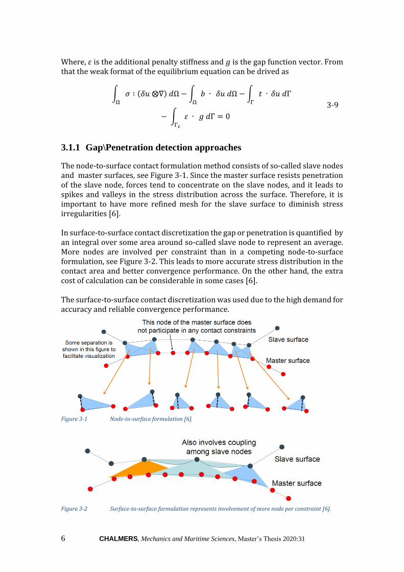
The node-to-surface contact formulation method consists of so-called slave nodes and master surfaces, see Figure 3-1. Since the master surface resists penetration of the slave node, forces tend to concentrate on the slave nodes, and it leads to spikes and valleys in the stress distribution across the surface. Therefore, it is important to have more refined mesh for the slave surface to diminish stress irregularities [6]. In surface-to-surface contact discretization the gap or penetration is quantified by an integral over some area around so-called slave node to represent an average. More nodes are involved per constraint than in a competing node-to-surface formulation, see Figure 3-2. This leads to more accurate stress distribution in the contact area and better convergence performance. On the other hand, the extra cost of calculation can be considerable in some cases [6]. The surface-to-surface contact discretization was used due to the high demand for accuracy and reliable convergence performance.
Figure 3-1 Node-to-surface formulation [6].
Figure 3-2 Surface-to-surface formulation represents involvement of more node per constraint [6].
CHALMERS, Mechanics and Maritime Sciences, Master’s Thesis 2020:31 7
3.1.2 Contact tracking approach
The finite-sliding tracking approach allows the contact surfaces for arbitrary relative separation, sliding, and rotation. In this approach, the contact constraints are updated in case of tangential motion of the contact surfaces. On the other hand, the small-sliding tracking approach assumes little sliding between the surfaces, and the contact constraint groups are fixed during the analysis. This will reduce the computational cost and reduce accuracy [6]. Due to the aim of modelling the stick- slip events the small-sliding approach causes nonphysical behaviour. Therefore, a finite-sliding approach for tracking was used.
3.1.3 Sticking constitutive equation
Two contact surfaces are under sticking condition when relative tangential velocity is zero. This condition can be obtained from as
𝑔�̇� = 0 ⇔ 𝑔𝑇 = 𝐶𝑜𝑛𝑠𝑡𝑎𝑛𝑡 3-10
This condition imposes a nonlinear constraint equation on the motion due to contact constraint that is further discussed in section 3.1.6.
3.1.4 Coulomb Friction
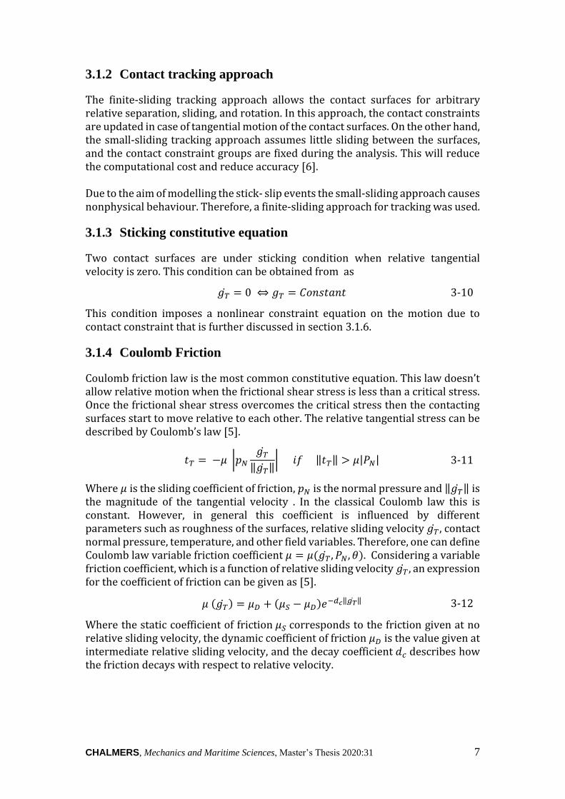
Coulomb friction law is the most common constitutive equation. This law doesn’t allow relative motion when the frictional shear stress is less than a critical stress. Once the frictional shear stress overcomes the critical stress then the contacting surfaces start to move relative to each other. The relative tangential stress can be described by Coulomb’s law [5].
𝑡𝑇 = −𝜇 |𝑝𝑁
𝑔�̇�
‖𝑔�̇�‖| 𝑖𝑓 ‖𝑡𝑇‖ > 𝜇|𝑃𝑁| 3-11
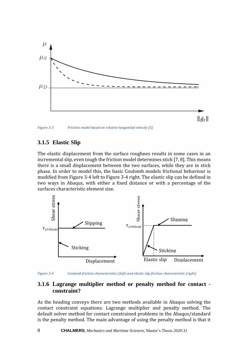
Where 𝜇 is the sliding coefficient of friction, 𝑝𝑁 is the normal pressure and ‖𝑔�̇�‖ is the magnitude of the tangential velocity . In the classical Coulomb law this is constant. However, in general this coefficient is influenced by different parameters such as roughness of the surfaces, relative sliding velocity 𝑔�̇� , contact normal pressure, temperature, and other field variables. Therefore, one can define Coulomb law variable friction coefficient 𝜇 = 𝜇(𝑔�̇� , 𝑃𝑁, 𝜃). Considering a variable friction coefficient, which is a function of relative sliding velocity 𝑔�̇� , an expression for the coefficient of friction can be given as [5].
𝜇 (𝑔�̇�) = 𝜇𝐷 + (𝜇𝑆 − 𝜇𝐷)𝑒−𝑑𝑐‖𝑔�̇�‖ 3-12
Where the static coefficient of friction 𝜇𝑆 corresponds to the friction given at no relative sliding velocity, the dynamic coefficient of friction 𝜇𝐷 is the value given at intermediate relative sliding velocity, and the decay coefficient 𝑑𝑐 describes how the friction decays with respect to relative velocity.
8 CHALMERS, Mechanics and Maritime Sciences, Master’s Thesis 2020:31
3.1.5 Elastic Slip
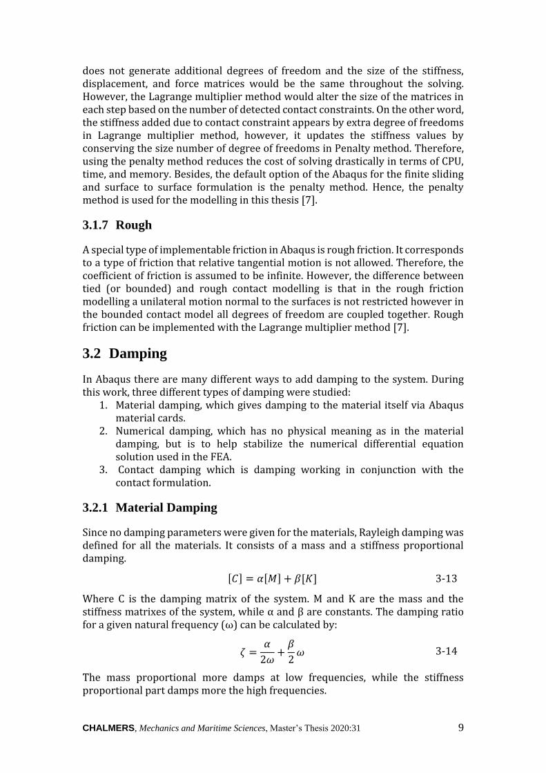
The elastic displacement from the surface roughnes results in some cases in an incremental slip, even tough the friction model determines stick [7, 8]. This means there is a small displacement between the two surfaces, while they are in stick phase. In order to model this, the basic Coulomb models frictional behaviour is modified from Figure 3-4 left to Figure 3-4 right. The elastic slip can be defined in two ways in Abaqus, with either a fixed distance or with a percentage of the surfaces characteristic element size.
Figure 3-4 Coulomb friction characteristics (left) and elastic slip friction characteristic (right)
3.1.6 Lagrange multiplier method or penalty method for contact -
constraint?
As the heading conveys there are two methods available in Abaqus solving the contact constraint equations: Lagrange multiplier and penalty method. The default solver method for contact constrained problems in the Abaqus/standard is the penalty method. The main advantage of using the penalty method is that it
Slipping
Sticking
Shea
r st
ress
𝜏𝑐𝑟𝑖𝑡𝑖𝑐𝑎𝑙
Displacement
Slipping
Sticking
Shea
r st
ress
𝜏𝑐𝑟𝑖𝑡𝑖𝑐𝑎𝑙
Displacement Elastic slip
‖𝑔�̇�‖
Figure 3-3 Friction model based on relative tangential velocity [5]
CHALMERS, Mechanics and Maritime Sciences, Master’s Thesis 2020:31 9
does not generate additional degrees of freedom and the size of the stiffness, displacement, and force matrices would be the same throughout the solving. However, the Lagrange multiplier method would alter the size of the matrices in each step based on the number of detected contact constraints. On the other word, the stiffness added due to contact constraint appears by extra degree of freedoms in Lagrange multiplier method, however, it updates the stiffness values by conserving the size number of degree of freedoms in Penalty method. Therefore, using the penalty method reduces the cost of solving drastically in terms of CPU, time, and memory. Besides, the default option of the Abaqus for the finite sliding and surface to surface formulation is the penalty method. Hence, the penalty method is used for the modelling in this thesis [7].
3.1.7 Rough
A special type of implementable friction in Abaqus is rough friction. It corresponds to a type of friction that relative tangential motion is not allowed. Therefore, the coefficient of friction is assumed to be infinite. However, the difference between tied (or bounded) and rough contact modelling is that in the rough friction modelling a unilateral motion normal to the surfaces is not restricted however in the bounded contact model all degrees of freedom are coupled together. Rough friction can be implemented with the Lagrange multiplier method [7].
3.2 Damping
In Abaqus there are many different ways to add damping to the system. During this work, three different types of damping were studied:
1. Material damping, which gives damping to the material itself via Abaqus material cards.
2. Numerical damping, which has no physical meaning as in the material damping, but is to help stabilize the numerical differential equation solution used in the FEA.
3. Contact damping which is damping working in conjunction with the contact formulation.
3.2.1 Material Damping
Since no damping parameters were given for the materials, Rayleigh damping was defined for all the materials. It consists of a mass and a stiffness proportional damping.
[𝐶] = 𝛼[𝑀] + 𝛽[𝐾] 3-13
Where C is the damping matrix of the system. M and K are the mass and the stiffness matrixes of the system, while α and β are constants. The damping ratio for a given natural frequency (ω) can be calculated by:
휁 =
𝛼
2𝜔+
𝛽
2𝜔 3-14
The mass proportional more damps at low frequencies, while the stiffness proportional part damps more the high frequencies.
10 CHALMERS, Mechanics and Maritime Sciences, Master’s Thesis 2020:31
The damping ratio was calculated with the help of the logarithmic decrement [9].
휁 =
𝛿
√4𝜋2 + 𝛿2 3-15
Where 𝛿 is the logarithmic decrement, and can be calculated by the following from a damped signal 𝑥(𝑡).
𝛿 =
1
𝑛𝑙𝑛 (
𝑥(𝑡)
𝑥(𝑡 + 𝑛𝑇)) 3-16
Where 𝑛𝜖ℤ is the number of periods between 𝑥(𝑡) and 𝑥(𝑡 + 𝑛𝑇), while T is the time for one period. The logarithmic decrement can be calculated for different eigenmodes.
3.2.2 Numerical Damping
In the implicit solver, the operator matrix converts to a set of nonlinear equilibrium equations that must be solved simultaneously in each time increment. The advantage of an implicit solver is the fact that it can be made unconditionally stable and it results in much lower computational cost comparing to an explicit solver that is only conditionally stable. However, solving these equations with a finite time step introduces numerical damping. The effect of numerical damping is specially considerable in contact conditions since changes in contact conditions can result in undesirable negative damping. The Hibler, Hughes and Taylor operator for numerical damping is used in Abaqus. Three parameter has been used in this model 𝛼𝑛, 𝛽𝑛 𝑎𝑛𝑑 𝛾𝑛. By modifying 𝛼 other parameters will be adjusted based on .
𝛽𝑛 =1
4 ∙ (1 − 𝛼𝑛)2 3-17
𝛾𝑛 =
1
2− 𝛼𝑛 3-18
This model introduces numerical damping on time integrator by preserving the characteristic of integrator. The amount damping depends on the size of the time
increment. When 𝛼𝑛 is zero ( 𝛽𝑛 =1
4 and 𝛾𝑛 =
1
2 , Newmark 𝛽𝑛 method) it is
equivalent to no damping and negative 𝛼𝑛 results in damping in the system.
Maximum damping is obtained at 𝛼𝑛 = −1
3 . The allowable range for 𝛼𝑛, 𝛽𝑛 and 𝛾𝑛
are −1
2≤ 𝛼𝑛 ≤ 0, 𝛽𝑛 > 0 and 𝛾𝑛 ≥
1
2 [7].
3.2.3 Contact Damping
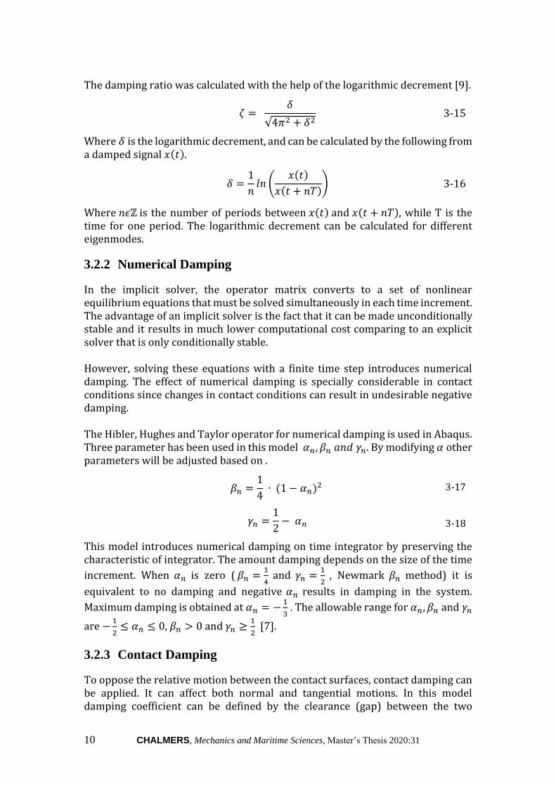
To oppose the relative motion between the contact surfaces, contact damping can be applied. It can affect both normal and tangential motions. In this model damping coefficient can be defined by the clearance (gap) between the two
CHALMERS, Mechanics and Maritime Sciences, Master’s Thesis 2020:31 11
surfaces, see Figure 3-5. To clarify the the effect of contact damping on the model, considering the system in Figure 3-5, the dynamic equations can be drived as
𝑚1�̈�1 − 𝑐𝑐(�̇�2 − �̇�1) + 𝑘𝑐(𝑥1 − 𝑥2) + 𝑘1𝑥1 = 𝑚1𝑔 3-19
𝑚2�̈�2 − 𝑐𝑐(�̇�2 − �̇�1) + 𝑘𝑐(𝑥1 − 𝑥2) + 𝑘2𝑥2 = 𝑚2𝑔 3-20
The characteristic equation can be written as following
|−𝑚1𝜔2 + 𝑗𝑐𝑐𝜔 + 𝑘𝑐 + 𝑘1 −𝑗𝑐𝑐𝜔 − 𝑘𝑐
−𝑗𝑐𝑐𝜔 − 𝑘𝑐 −𝑚2𝜔2 + 𝑗𝑐𝑐𝜔 + 𝑘𝑐 + 𝑘2
| = 0 3-21
𝑘𝑐 = 𝑚1𝑚2𝜔4 − (𝑚1𝑘2 + 𝑚2𝑘1)𝜔2 + 𝑘1𝑘2
(𝑚1 + 𝑚2)𝜔2 − (𝑘1 + 𝑘2)− 𝑗𝑐𝑐𝜔
3-22
The root of the characteristic equation, 𝜔 is a complex number, due to the contact damping. It physically means that because of contact damping there is some signal decay. A parametric study was performed to investigate this effect on the CAE model.
Figure 3-5 Damping coefficient definition (left) System model (right) [10]
3.3 Dynamic Substructuring
Substructures are structures that interact with the neighboring structures. Dynamic substructuring gives the possibility of combining modeled parts [11]. By creating a substructure (which is called super-element in Abaqus) the computational costs can be reduced significantly, while still having accurate results. This can be reached by defining a part of the system as a substructure, and decrease its degrees of freedom by finding the dynamic behaviour of the substructure [12]. Much research has been done in this field and could be a separate thesis. In this work the scope is not on dynamic substructuring, but more of a tool used. However, the theory behind it will be presented shortly: This thesis used one of the most popular Compoent Mode Synthethis (CMS) methods, the Craig-Bampton method. CMS decomposes the system into substructures, which are analised separately then reduced and simplified before reassembling [11-13]. The Craig-Bampton method uses fixed interface vibration modes together with static condensation modes, also known as Guyan modes [13, 14].
12 CHALMERS, Mechanics and Maritime Sciences, Master’s Thesis 2020:31
The Guyan modes removes all internal Defree of Freedoms (DOFs) of the substructure, and retains only the DoFs connecting the substructure to the main or the rest of the. These so called interface DoFs are part of both of the main and the substructures system. The response associated to a unit displacement to each interface DoF, while the other interface DoFs are constrained is captured in the Guyan mode matrix [13, 15, 16]. However, to capture the dynamic behaviour of the system the Guyan modes are not enough. Therefore the fixed interface vibration modes has to be included. Similarly to the Guyan modes, this technique also reduses the internal DoFs of the substructure by creating the so called generalised DoFs, which captures the systems response with less DoFs [13]. As mentioned before, the Craig-Bampton method uses a so called reduction matrix consisting of a combination Guyan modes and the fixed interface vibration modes [14].
CHALMERS, Mechanics and Maritime Sciences, Master’s Thesis 2020:31 13
4 Physical Tests
The current thesis is based on experiments done with the Ziegler ssp-04 stick-slip machine. The FEM is based on a subpart of this machine.
4.1 Experimental setup: The Ziegler ssp-04
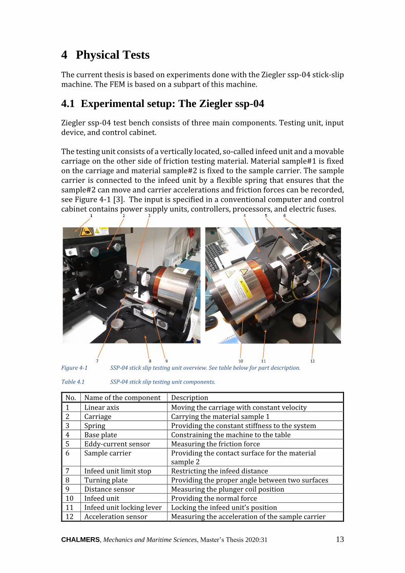
Ziegler ssp-04 test bench consists of three main components. Testing unit, input device, and control cabinet. The testing unit consists of a vertically located, so-called infeed unit and a movable carriage on the other side of friction testing material. Material sample#1 is fixed on the carriage and material sample#2 is fixed to the sample carrier. The sample carrier is connected to the infeed unit by a flexible spring that ensures that the sample#2 can move and carrier accelerations and friction forces can be recorded, see Figure 4-1 [3]. The input is specified in a conventional computer and control cabinet contains power supply units, controllers, processors, and electric fuses.
Figure 4-1 SSP-04 stick slip testing unit overview. See table below for part description.
Table 4.1 SSP-04 stick slip testing unit components.
No. Name of the component Description
1 Linear axis Moving the carriage with constant velocity 2 Carriage Carrying the material sample 1 3 Spring Providing the constant stiffness to the system 4 Base plate Constraining the machine to the table 5 Eddy-current sensor Measuring the friction force 6 Sample carrier Providing the contact surface for the material
sample 2 7 Infeed unit limit stop Restricting the infeed distance 8 Turning plate Providing the proper angle between two surfaces 9 Distance sensor Measuring the plunger coil position 10 Infeed unit Providing the normal force 11 Infeed unit locking lever Locking the infeed unit’s position 12 Acceleration sensor Measuring the acceleration of the sample carrier
14 CHALMERS, Mechanics and Maritime Sciences, Master’s Thesis 2020:31
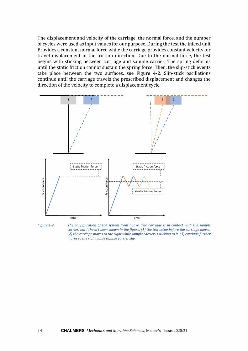
The displacement and velocity of the carriage, the normal force, and the number of cycles were used as input values for our purpose. During the test the infeed unit Provides a constant normal force while the carriage provides constant velocity for travel displacement in the friction direction. Due to the normal force, the test begins with sticking between carriage and sample carrier. The spring deforms until the static friction cannot sustain the spring force. Then, the slip-stick events take place between the two surfaces, see Figure 4-2. Slip-stick oscillations continue until the carriage travels the prescribed displacement and changes the direction of the velocity to complete a displacement cycle.
Figure 4-2 The configuration of the system from above. The carriage is in contact with the sample
carrier, but it hasn’t been shown in the figure. (1) the test setup before the carriage moves. (2) the carriage moves to the right while sample carrier is sticking to it. (3) carriage further moves to the right while sample carrier slip.
CHALMERS, Mechanics and Maritime Sciences, Master’s Thesis 2020:31 15
4.2 Experiment’s Outputs
Acceleration and eddy-current sensors record the carrier acceleration and friction force signals. After postprocessing on these signals, the other parameters are calculated and compared with the Ziegler database. Those parameters are shown in Table 4.2. Table 4.2 Experiment Outputs
Parameters Description
Maximum acceleration Maximum of acceleration signal Impulse value Number of impulses during the measurement Impulse rate Impulse vale divided into the displacement Static friction force Maximum friction force just before surfaces start to
move with respect to each other (Stick) Dynamic friction force Friction force correspond to the time surfaces slip
with respect to each other. Static friction coefficient Static friction force devided by normal force Dynamic friction coefficient Dynamic friction force devided by normal force Risk Probability Number (RPN)
Risk priority index: The Risk Priority index or the Risk Priority Number is a machine output and during this work it is treated as a black box.
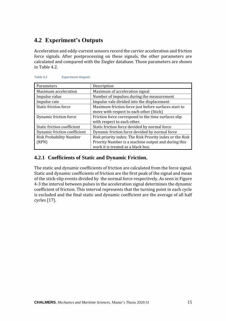
4.2.1 Coefficients of Static and Dynamic Friction.
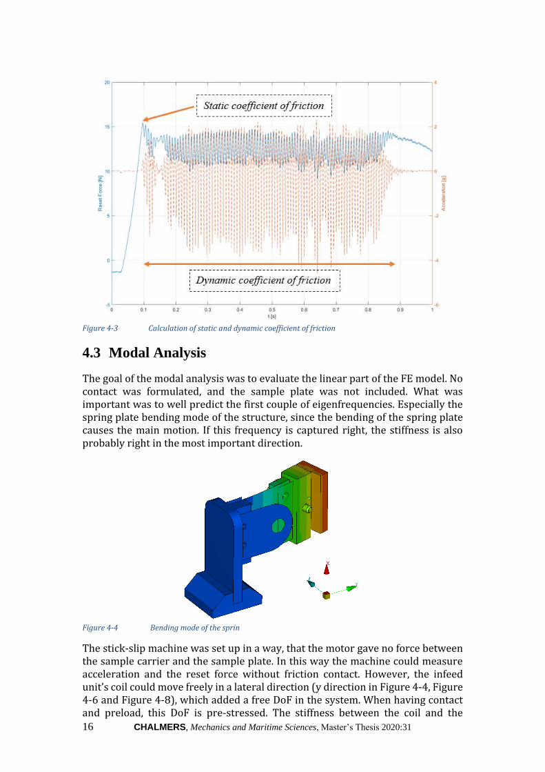
The static and dynamic coefficients of friction are calculated from the force signal. Static and dynamic coefficients of friction are the first peak of the signal and mean of the stick-slip events divided by the normal force respectively. As seen in Figure 4-3 the interval between pulses in the acceleration signal determines the dynamic coefficient of friction. This interval represents that the turning point in each cycle is excluded and the final static and dynamic coefficient are the average of all half cycles [17].
16 CHALMERS, Mechanics and Maritime Sciences, Master’s Thesis 2020:31
Figure 4-3 Calculation of static and dynamic coefficient of friction
4.3 Modal Analysis
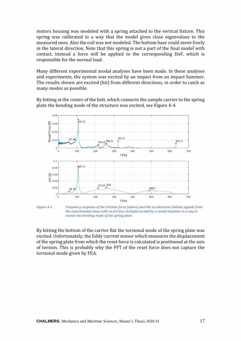
The goal of the modal analysis was to evaluate the linear part of the FE model. No contact was formulated, and the sample plate was not included. What was important was to well predict the first couple of eigenfrequencies. Especially the spring plate bending mode of the structure, since the bending of the spring plate causes the main motion. If this frequency is captured right, the stiffness is also probably right in the most important direction.
Figure 4-4 Bending mode of the sprin
The stick-slip machine was set up in a way, that the motor gave no force between the sample carrier and the sample plate. In this way the machine could measure acceleration and the reset force without friction contact. However, the infeed unit’s coil could move freely in a lateral direction (y direction in Figure 4-4, Figure 4-6 and Figure 4-8), which added a free DoF in the system. When having contact and preload, this DoF is pre-stressed. The stiffness between the coil and the
CHALMERS, Mechanics and Maritime Sciences, Master’s Thesis 2020:31 17
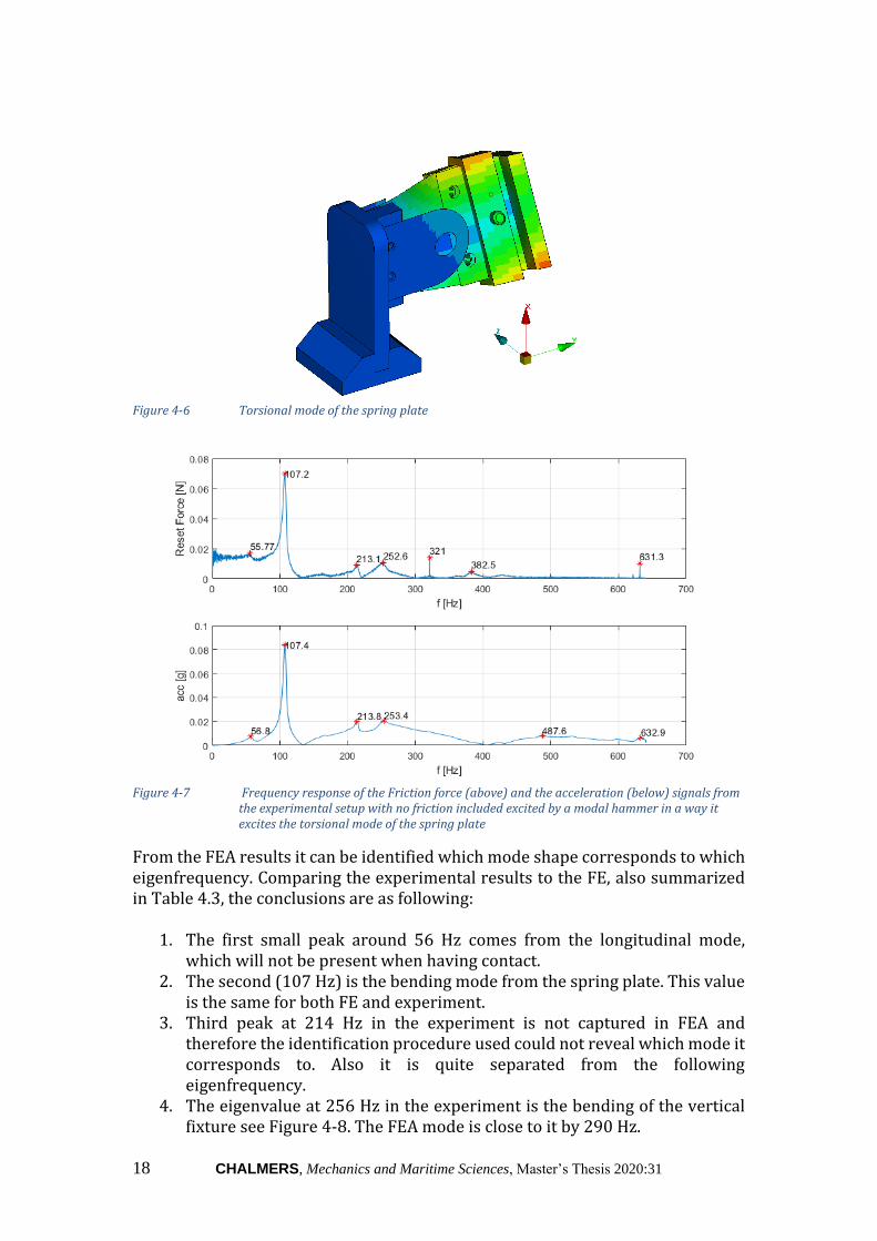
motors housing was modeled with a spring attached to the vertical fixture. This spring was calibrated in a way that the model gives close eigenvalues to the measured ones. Also the coil was not modeled. The bottom base could move freely in the lateral direction. Note that this spring is not a part of the final model with contact. Instead a force will be applied to the corresponding DoF, which is responsible for the normal load. Many different experimental modal analyses have been made. In these analyses and experiments, the system was excited by an impact from an impact hammer. The results shown are excited (hit) from different directions, in order to catch as many modes as possible. By hitting at the center of the bolt, which connects the sample carrier to the spring plate the bending mode of the structure was excited, see Figure 4-4.
Figure 4-5 Frequency response of the Friction force (above) and the acceleration (below) signals from
the experimental setup with no friction included excited by a modal hammer in a way it excites the bending mode of the spring plate
By hitting the bottom of the carrier flat the torsional mode of the spring plate was excited. Unfortunately, the Eddy current sensor which measures the displacement of the spring plate from which the reset force is calculated is positioned at the axis of torsion. This is probably why the FFT of the reset force does not capture the torsional mode given by FEA.
18 CHALMERS, Mechanics and Maritime Sciences, Master’s Thesis 2020:31
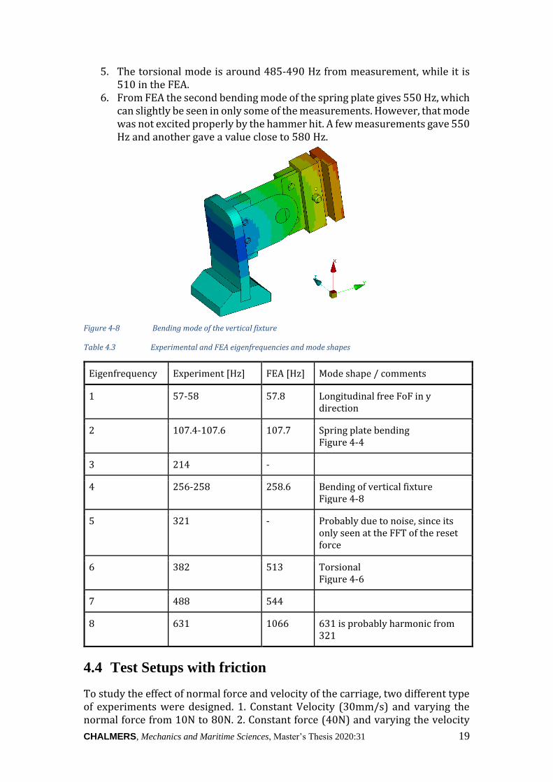
Figure 4-6 Torsional mode of the spring plate
Figure 4-7 Frequency response of the Friction force (above) and the acceleration (below) signals from
the experimental setup with no friction included excited by a modal hammer in a way it excites the torsional mode of the spring plate
From the FEA results it can be identified which mode shape corresponds to which eigenfrequency. Comparing the experimental results to the FE, also summarized in Table 4.3, the conclusions are as following:
1. The first small peak around 56 Hz comes from the longitudinal mode, which will not be present when having contact.
2. The second (107 Hz) is the bending mode from the spring plate. This value is the same for both FE and experiment.
3. Third peak at 214 Hz in the experiment is not captured in FEA and therefore the identification procedure used could not reveal which mode it corresponds to. Also it is quite separated from the following eigenfrequency.
4. The eigenvalue at 256 Hz in the experiment is the bending of the vertical fixture see Figure 4-8. The FEA mode is close to it by 290 Hz.
CHALMERS, Mechanics and Maritime Sciences, Master’s Thesis 2020:31 19
5. The torsional mode is around 485-490 Hz from measurement, while it is 510 in the FEA.
6. From FEA the second bending mode of the spring plate gives 550 Hz, which can slightly be seen in only some of the measurements. However, that mode was not excited properly by the hammer hit. A few measurements gave 550 Hz and another gave a value close to 580 Hz.
Figure 4-8 Bending mode of the vertical fixture
Table 4.3 Experimental and FEA eigenfrequencies and mode shapes
Eigenfrequency Experiment [Hz] FEA [Hz] Mode shape / comments
1 57-58 57.8 Longitudinal free FoF in y direction
2 107.4-107.6 107.7 Spring plate bending Figure 4-4
3 214 -
4 256-258 258.6 Bending of vertical fixture Figure 4-8
5 321 - Probably due to noise, since its only seen at the FFT of the reset force
6 382 513 Torsional Figure 4-6
7 488 544
8 631 1066 631 is probably harmonic from 321
4.4 Test Setups with friction
To study the effect of normal force and velocity of the carriage, two different type of experiments were designed. 1. Constant Velocity (30mm/s) and varying the normal force from 10N to 80N. 2. Constant force (40N) and varying the velocity
20 CHALMERS, Mechanics and Maritime Sciences, Master’s Thesis 2020:31
from 3 mm/s to 70 mm/s. 4 Different material combination based on their importance were chosen. Section 7.2 illustrates the trend of output parameters in for these experiment with different material combinations. PP stands for Polypropylene, AL for aluminium and PCABS for Polycarbonate-
Acrylonitrile Butadiene Styrene. It is important to mention, that the following results
are oututs from the Zeigler instrument, and the values are calculated for the whole
signal. Since the signalis not symmetric the values cannot be corresponded exactly to
the FEA results, however the trends should be similar.
4.4.1 Constant Force
In the following results the normal force was was kept constant at 40 N, while the velocity was changed:
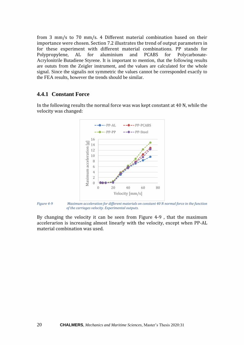
Figure 4-9 Maximum acceleration for different materials on constant 40 N normal force in the function
of the carriages velocity. Experimental outputs.
By changing the velocity it can be seen from Figure 4-9 , that the maximum accelerarion is increasing almost linearly with the velocity, except when PP-AL material combination was used.
0
2
4
6
8
10
12
14
16
0 20 40 60 80
Max
imu
m a
ccel
erat
ion
[g]
Velocity [mm/s]
PP-AL PP-PCABS
PP-PP PP-Steel
CHALMERS, Mechanics and Maritime Sciences, Master’s Thesis 2020:31 21
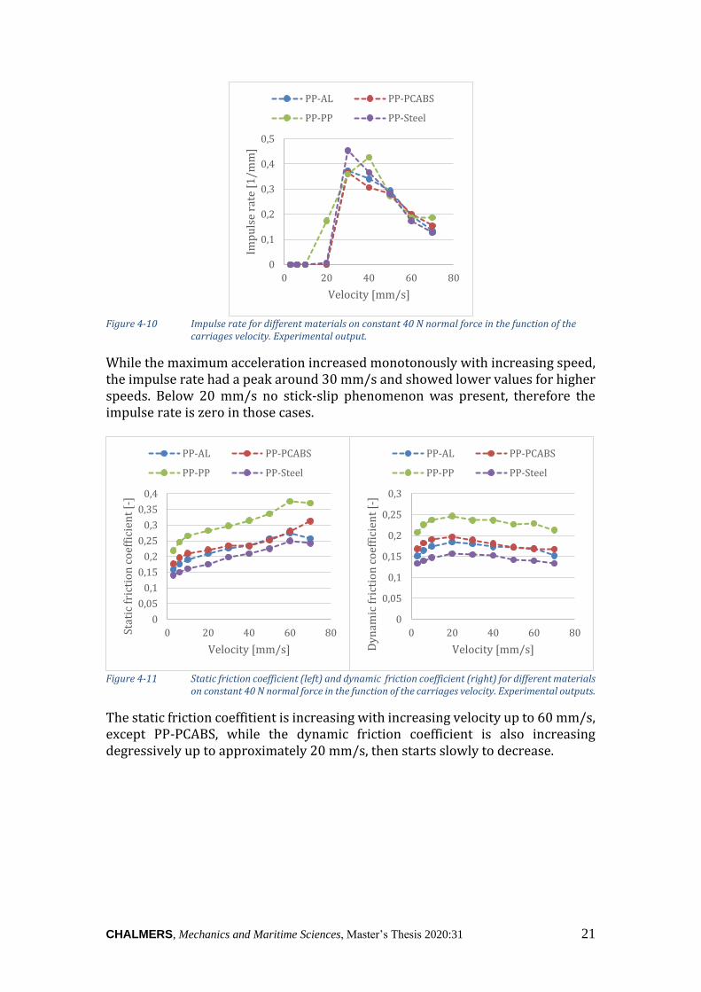
Figure 4-10 Impulse rate for different materials on constant 40 N normal force in the function of the
carriages velocity. Experimental output.
While the maximum acceleration increased monotonously with increasing speed, the impulse rate had a peak around 30 mm/s and showed lower values for higher speeds. Below 20 mm/s no stick-slip phenomenon was present, therefore the impulse rate is zero in those cases.
Figure 4-11 Static friction coefficient (left) and dynamic friction coefficient (right) for different materials
on constant 40 N normal force in the function of the carriages velocity. Experimental outputs.
The static friction coeffitient is increasing with increasing velocity up to 60 mm/s, except PP-PCABS, while the dynamic friction coefficient is also increasing degressively up to approximately 20 mm/s, then starts slowly to decrease.
0
0,1
0,2
0,3
0,4
0,5
0 20 40 60 80
Imp
uls
e ra
te [
1/m
m]
Velocity [mm/s]
PP-AL PP-PCABS
PP-PP PP-Steel
0
0,05
0,1
0,15
0,2
0,25
0,3
0,35
0,4
0 20 40 60 80Stat
ic f
rict
ion
co
effi
cien
t [-
]
Velocity [mm/s]
PP-AL PP-PCABS
PP-PP PP-Steel
0
0,05
0,1
0,15
0,2
0,25
0,3
0 20 40 60 80
Dy
nam
ic f
rict
ion
co
effi
cien
t [-
]
Velocity [mm/s]
PP-AL PP-PCABS
PP-PP PP-Steel
22 CHALMERS, Mechanics and Maritime Sciences, Master’s Thesis 2020:31
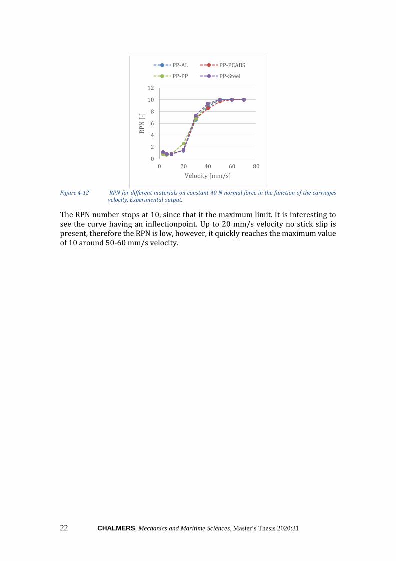
Figure 4-12 RPN for different materials on constant 40 N normal force in the function of the carriages
velocity. Experimental output.
The RPN number stops at 10, since that it the maximum limit. It is interesting to see the curve having an inflectionpoint. Up to 20 mm/s velocity no stick slip is present, therefore the RPN is low, however, it quickly reaches the maximum value of 10 around 50-60 mm/s velocity.
0
2
4
6
8
10
12
0 20 40 60 80
RP
N [
-]
Velocity [mm/s]
PP-AL PP-PCABS
PP-PP PP-Steel
CHALMERS, Mechanics and Maritime Sciences, Master’s Thesis 2020:31 23
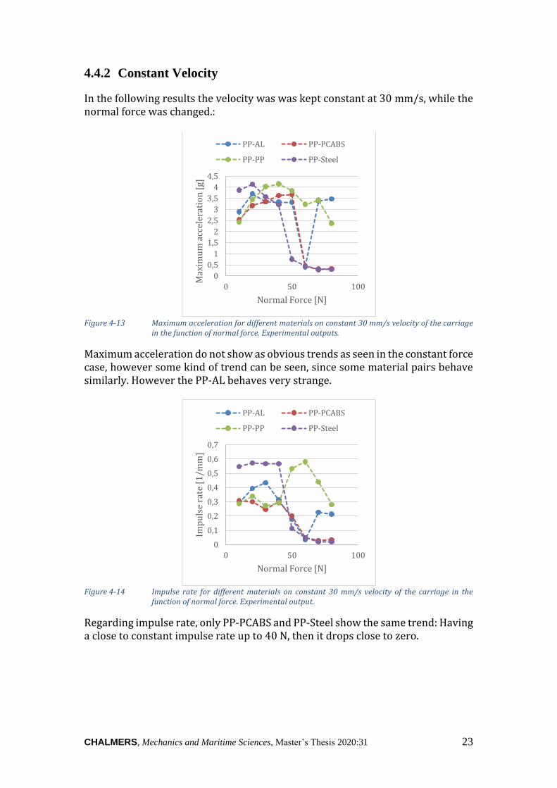
4.4.2 Constant Velocity
In the following results the velocity was was kept constant at 30 mm/s, while the normal force was changed.:
Figure 4-13 Maximum acceleration for different materials on constant 30 mm/s velocity of the carriage
in the function of normal force. Experimental outputs.
Maximum acceleration do not show as obvious trends as seen in the constant force case, however some kind of trend can be seen, since some material pairs behave similarly. However the PP-AL behaves very strange.
Figure 4-14 Impulse rate for different materials on constant 30 mm/s velocity of the carriage in the
function of normal force. Experimental output.
Regarding impulse rate, only PP-PCABS and PP-Steel show the same trend: Having a close to constant impulse rate up to 40 N, then it drops close to zero.
0
0,5
1
1,5
2
2,5
3
3,5
4
4,5
0 50 100
Max
imu
m a
ccel
erat
ion
[g]
Normal Force [N]
PP-AL PP-PCABS
PP-PP PP-Steel
0
0,1
0,2
0,3
0,4
0,5
0,6
0,7
0 50 100
Imp
uls
e ra
te [
1/m
m]
Normal Force [N]
PP-AL PP-PCABS
PP-PP PP-Steel
24 CHALMERS, Mechanics and Maritime Sciences, Master’s Thesis 2020:31
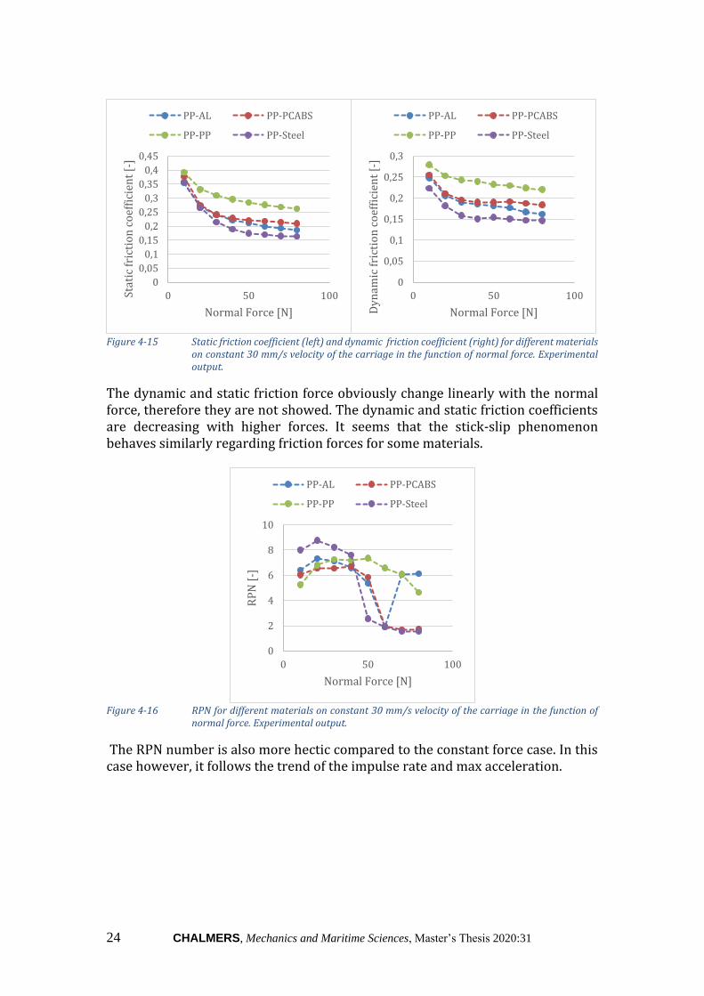
Figure 4-15 Static friction coefficient (left) and dynamic friction coefficient (right) for different materials
on constant 30 mm/s velocity of the carriage in the function of normal force. Experimental output.
The dynamic and static friction force obviously change linearly with the normal force, therefore they are not showed. The dynamic and static friction coefficients are decreasing with higher forces. It seems that the stick-slip phenomenon behaves similarly regarding friction forces for some materials.
Figure 4-16 RPN for different materials on constant 30 mm/s velocity of the carriage in the function of
normal force. Experimental output.
The RPN number is also more hectic compared to the constant force case. In this case however, it follows the trend of the impulse rate and max acceleration.
0
0,05
0,1
0,15
0,2
0,25
0,3
0,35
0,4
0,45
0 50 100Stat
ic f
rict
ion
co
effi
cien
t [-
]
Normal Force [N]
PP-AL PP-PCABS
PP-PP PP-Steel
0
0,05
0,1
0,15
0,2
0,25
0,3
0 50 100
Dy
nam
ic f
rict
ion
co
effi
cien
t [-
]
Normal Force [N]
PP-AL PP-PCABS
PP-PP PP-Steel
0
2
4
6
8
10
0 50 100
RP
N [
-]
Normal Force [N]
PP-AL PP-PCABS
PP-PP PP-Steel
CHALMERS, Mechanics and Maritime Sciences, Master’s Thesis 2020:31 25
5 FEM Implementation
5.1 Abaqus
During the study ABAQUS/standard implicit solver was used for time domain simulations as well as for modal analysis with eigenvalue exctraction.
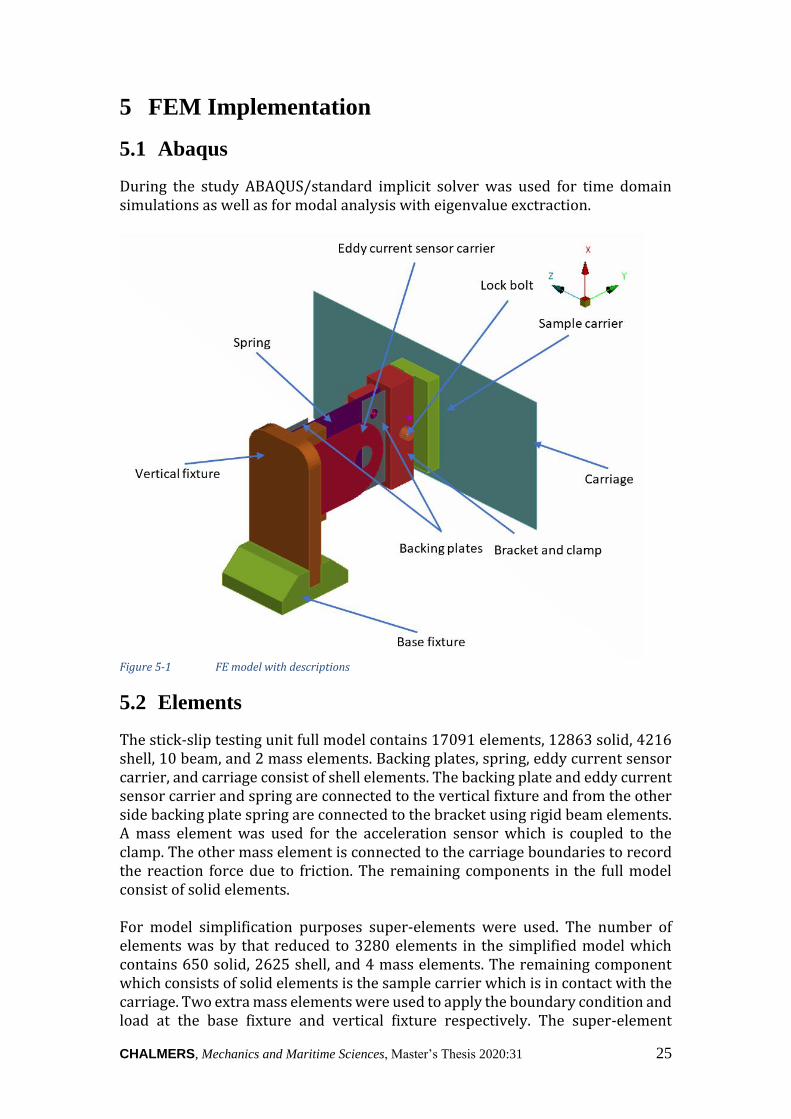
Figure 5-1 FE model with descriptions
5.2 Elements
The stick-slip testing unit full model contains 17091 elements, 12863 solid, 4216 shell, 10 beam, and 2 mass elements. Backing plates, spring, eddy current sensor carrier, and carriage consist of shell elements. The backing plate and eddy current sensor carrier and spring are connected to the vertical fixture and from the other side backing plate spring are connected to the bracket using rigid beam elements. A mass element was used for the acceleration sensor which is coupled to the clamp. The other mass element is connected to the carriage boundaries to record the reaction force due to friction. The remaining components in the full model consist of solid elements. For model simplification purposes super-elements were used. The number of elements was by that reduced to 3280 elements in the simplified model which contains 650 solid, 2625 shell, and 4 mass elements. The remaining component which consists of solid elements is the sample carrier which is in contact with the carriage. Two extra mass elements were used to apply the boundary condition and load at the base fixture and vertical fixture respectively. The super-element
26 CHALMERS, Mechanics and Maritime Sciences, Master’s Thesis 2020:31
substructure is connected to the solid element of the sample carrier using a multipoint constraint.
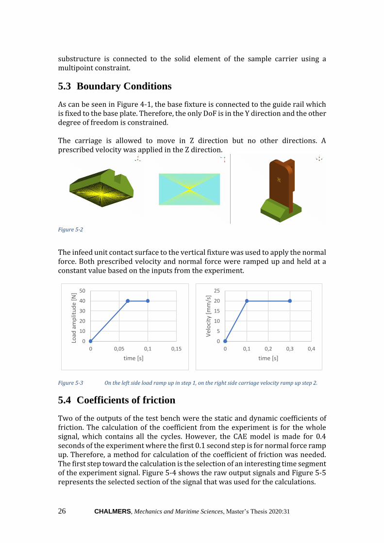
5.3 Boundary Conditions
As can be seen in Figure 4-1, the base fixture is connected to the guide rail which is fixed to the base plate. Therefore, the only DoF is in the Y direction and the other degree of freedom is constrained. The carriage is allowed to move in Z direction but no other directions. A prescribed velocity was applied in the Z direction.
Figure 5-2
The infeed unit contact surface to the vertical fixture was used to apply the normal force. Both prescribed velocity and normal force were ramped up and held at a constant value based on the inputs from the experiment.
Figure 5-3 On the left side load ramp up in step 1, on the right side carriage velocity ramp up step 2.
5.4 Coefficients of friction
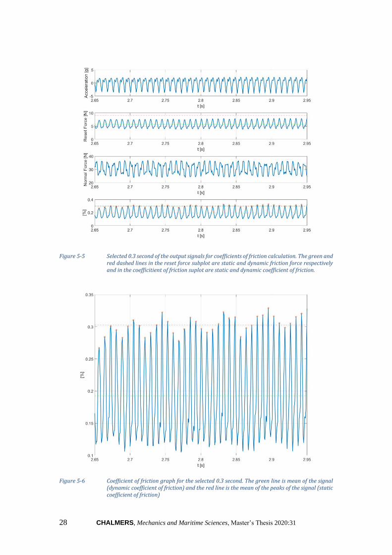
Two of the outputs of the test bench were the static and dynamic coefficients of friction. The calculation of the coefficient from the experiment is for the whole signal, which contains all the cycles. However, the CAE model is made for 0.4 seconds of the experiment where the first 0.1 second step is for normal force ramp up. Therefore, a method for calculation of the coefficient of friction was needed. The first step toward the calculation is the selection of an interesting time segment of the experiment signal. Figure 5-4 shows the raw output signals and Figure 5-5 represents the selected section of the signal that was used for the calculations.
0
10
20
30
40
50
0 0,05 0,1 0,15
Load
am
plit
ud
e [N
]
time [s]
0
5
10
15
20
25
0 0,1 0,2 0,3 0,4
Vel
oci
ty [
mm
/s]
time [s]
CHALMERS, Mechanics and Maritime Sciences, Master’s Thesis 2020:31 27
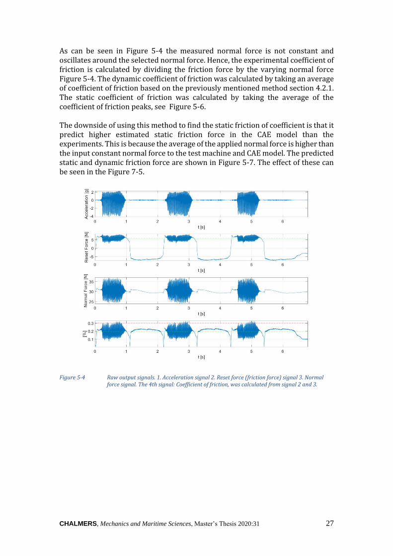
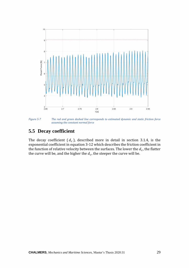
As can be seen in Figure 5-4 the measured normal force is not constant and oscillates around the selected normal force. Hence, the experimental coefficient of friction is calculated by dividing the friction force by the varying normal force Figure 5-4. The dynamic coefficient of friction was calculated by taking an average of coefficient of friction based on the previously mentioned method section 4.2.1. The static coefficient of friction was calculated by taking the average of the coefficient of friction peaks, see Figure 5-6. The downside of using this method to find the static friction of coefficient is that it predict higher estimated static friction force in the CAE model than the experiments. This is because the average of the applied normal force is higher than the input constant normal force to the test machine and CAE model. The predicted static and dynamic friction force are shown in Figure 5-7. The effect of these can be seen in the Figure 7-5.
Figure 5-4 Raw output signals. 1. Acceleration signal 2. Reset force (friction force) signal 3. Normal
force signal. The 4th signal: Coefficient of friction, was calculated from signal 2 and 3.
28 CHALMERS, Mechanics and Maritime Sciences, Master’s Thesis 2020:31
Figure 5-5 Selected 0.3 second of the output signals for coefficients of friction calculation. The green and
red dashed lines in the reset force subplot are static and dynamic friction force respectively and in the coefficitient of friction suplot are static and dynamic coefficient of friction.
Figure 5-6 Coefficient of friction graph for the selected 0.3 second. The green line is mean of the signal
(dynamic coefficient of friction) and the red line is the mean of the peaks of the signal (static coefficient of friction)
CHALMERS, Mechanics and Maritime Sciences, Master’s Thesis 2020:31 29
Figure 5-7 The red and green dashed line corresponds to estimated dynamic and static friction force
assuming the constant normal force
5.5 Decay coefficient
The decay coefficient ( 𝑑𝑐 ), described more in detail in section 3.1.4, is the exponential coefficient in equation 3-12 which describes the friction coefficient in the function of relative velocity between the surfaces. The lower the 𝑑𝑐, the flatter the curve will be, and the higher the 𝑑𝑐, the steeper the curve will be.
30 CHALMERS, Mechanics and Maritime Sciences, Master’s Thesis 2020:31
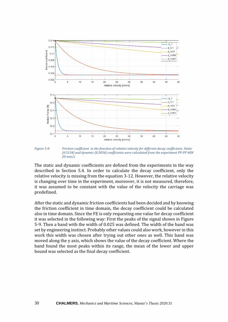
Figure 5-8 Friction coefficient in the function of relative velocity for different decay coefficients. Static
(0.3134) and dynamic (0.3034) coefficients were calculated from the experiment PP-PP 40N 20 mm/s
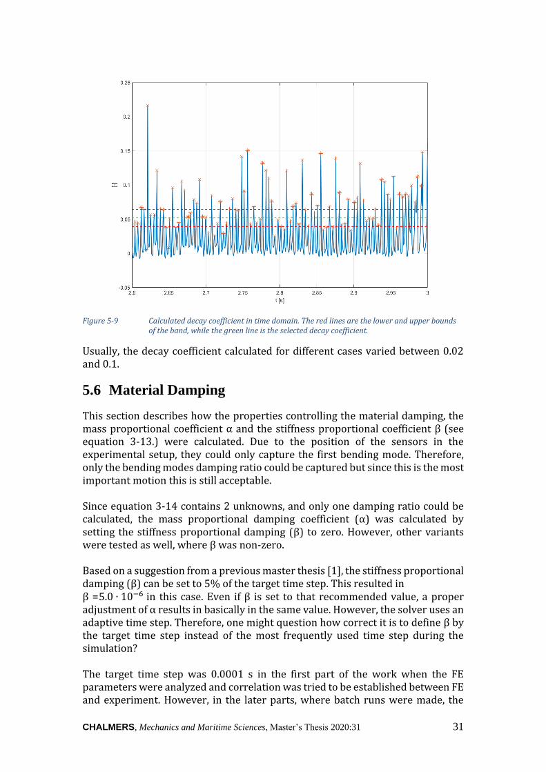
The static and dynamic coefficients are defined from the experiments in the way described in Section 5.4. In order to calculate the decay coefficient, only the relative velocity is missing from the equation 3-12. However, the relative velocity is changing over time in the experiment, moreover, it is not measured, therefore, it was assumed to be constant with the value of the velocity the carriage was predefined. After the static and dynamic friction coefficients had been decided and by knowing the friction coefficient in time domain, the decay coefficient could be calculated also in time domain. Since the FE is only requesting one value for decay coefficient it was selected in the following way: First the peaks of the signal shown in Figure 5-9. Then a band with the width of 0.025 was defined. The width of the band was set by engineering instinct. Probably other values could also work, however in this work this width was chosen after trying out other ones as well. This band was moved along the y axis, which shows the value of the decay coefficient. Where the band found the most peaks within its range, the mean of the lower and upper bound was selected as the final decay coefficient.
CHALMERS, Mechanics and Maritime Sciences, Master’s Thesis 2020:31 31
Figure 5-9 Calculated decay coefficient in time domain. The red lines are the lower and upper bounds
of the band, while the green line is the selected decay coefficient.
Usually, the decay coefficient calculated for different cases varied between 0.02 and 0.1.
5.6 Material Damping
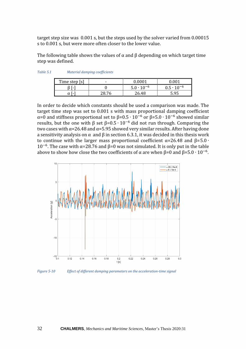
This section describes how the properties controlling the material damping, the mass proportional coefficient α and the stiffness proportional coefficient β (see equation 3-13.) were calculated. Due to the position of the sensors in the experimental setup, they could only capture the first bending mode. Therefore, only the bending modes damping ratio could be captured but since this is the most important motion this is still acceptable. Since equation 3-14 contains 2 unknowns, and only one damping ratio could be calculated, the mass proportional damping coefficient (α) was calculated by setting the stiffness proportional damping (β) to zero. However, other variants were tested as well, where β was non-zero. Based on a suggestion from a previous master thesis [1], the stiffness proportional damping (β) can be set to 5% of the target time step. This resulted in β =5.0 ∙ 10−6 in this case. Even if β is set to that recommended value, a proper adjustment of α results in basically in the same value. However, the solver uses an adaptive time step. Therefore, one might question how correct it is to define β by the target time step instead of the most frequently used time step during the simulation? The target time step was 0.0001 s in the first part of the work when the FE parameters were analyzed and correlation was tried to be established between FE and experiment. However, in the later parts, where batch runs were made, the
32 CHALMERS, Mechanics and Maritime Sciences, Master’s Thesis 2020:31
target step size was 0.001 s, but the steps used by the solver varied from 0.00015 s to 0.001 s, but were more often closer to the lower value. The following table shows the values of α and β depending on which target time step was defined. Table 5.1 Material damping coefficients
Time step [s] - 0.0001 0.001
β [-] 0 5.0 ∙ 10−6 0.5 ∙ 10−6 α [-] 28.76 26.48 5.95
In order to decide which constants should be used a comparison was made. The target time step was set to 0.001 s with mass proportional damping coefficient α=0 and stiffness proportional set to β=0.5 ∙ 10−6 or β=5.0 ∙ 10−6 showed similar results, but the one with β set β=0.5 ∙ 10−6 did not run through. Comparing the two cases with α=26.48 and α=5.95 showed very similar results. After having done a sensitivity analysis on α and β in section 6.3.1, it was decided in this thesis work to continue with the larger mass proportional coefficient α=26.48 and β=5.0 ∙10−6. The case with α=28.76 and β=0 was not simulated. It is only put in the table above to show how close the two coefficients of α are when β=0 and β=5.0 ∙ 10−6.
Figure 5-10 Effect of different damping parameters on the acceleration-time signal
CHALMERS, Mechanics and Maritime Sciences, Master’s Thesis 2020:31 33
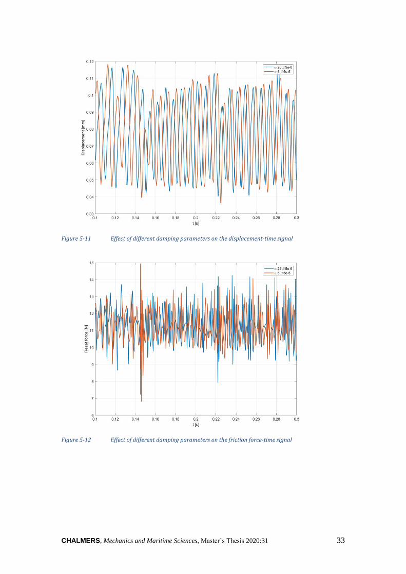
Figure 5-11 Effect of different damping parameters on the displacement-time signal
Figure 5-12 Effect of different damping parameters on the friction force-time signal
34 CHALMERS, Mechanics and Maritime Sciences, Master’s Thesis 2020:31
5.7 Dynamic Substructure
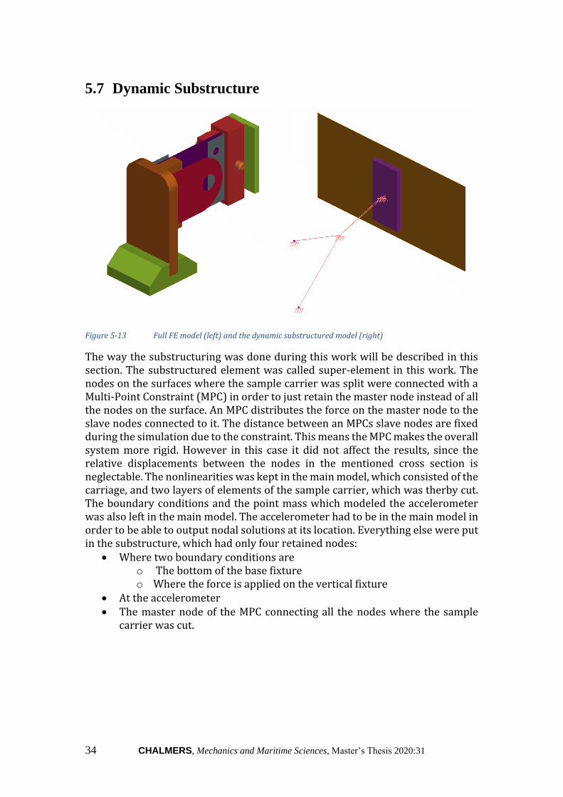
Figure 5-13 Full FE model (left) and the dynamic substructured model (right)
The way the substructuring was done during this work will be described in this section. The substructured element was called super-element in this work. The nodes on the surfaces where the sample carrier was split were connected with a Multi-Point Constraint (MPC) in order to just retain the master node instead of all the nodes on the surface. An MPC distributes the force on the master node to the slave nodes connected to it. The distance between an MPCs slave nodes are fixed during the simulation due to the constraint. This means the MPC makes the overall system more rigid. However in this case it did not affect the results, since the relative displacements between the nodes in the mentioned cross section is neglectable. The nonlinearities was kept in the main model, which consisted of the carriage, and two layers of elements of the sample carrier, which was therby cut. The boundary conditions and the point mass which modeled the accelerometer was also left in the main model. The accelerometer had to be in the main model in order to be able to output nodal solutions at its location. Everything else were put in the substructure, which had only four retained nodes:
• Where two boundary conditions are o The bottom of the base fixture o Where the force is applied on the vertical fixture
• At the accelerometer • The master node of the MPC connecting all the nodes where the sample
carrier was cut.
CHALMERS, Mechanics and Maritime Sciences, Master’s Thesis 2020:31 35
6 Parametric Investigation
In this section a study has been made regarding different FE parameters, and how they influence the results. All of the parameters were investigated on the PP-PP 40 N normal force 20 mm/s velocity case, and the following results are mostly done on this case. However many parameters were also investigated on other cases. It was only later realised, that the mentioned case is a boarderline case, where the stick-slip phenomenon happens, but the FE model does not capture it so well. The accelerations are 3 times higher in FE than in the experiment, therefore the results from this case was not captured in the batch simulations. Even though parameters were tuned based on a boarderline model, they were checked on other models as well. It would have been better to tune the parameters on a general case, not on a boarderline case, where the question arises, that can we simulate very low severity stick-slip cases, however this might not be a big mistake, since the trends of different parameters are still having the same effect. Very high severity stick-slip cases are also hard to simulate due to convergence issues.
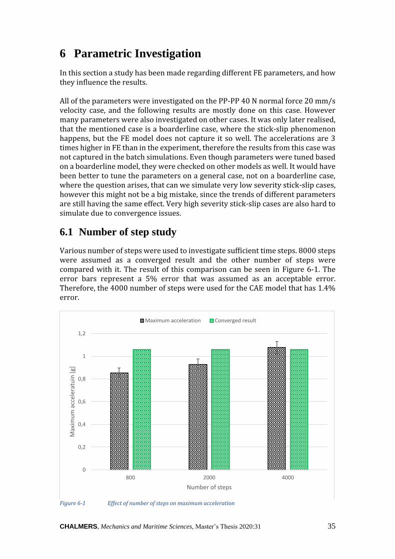
6.1 Number of step study
Various number of steps were used to investigate sufficient time steps. 8000 steps were assumed as a converged result and the other number of steps were compared with it. The result of this comparison can be seen in Figure 6-1. The error bars represent a 5% error that was assumed as an acceptable error. Therefore, the 4000 number of steps were used for the CAE model that has 1.4% error.
Figure 6-1 Effect of number of steps on maximum acceleration
0
0,2
0,4
0,6
0,8
1
1,2
800 2000 4000
Max
imu
m a
ccel
erat
uin
[g]
Number of steps
Maximum acceleration Converged result
36 CHALMERS, Mechanics and Maritime Sciences, Master’s Thesis 2020:31
6.2 Mesh Size Study
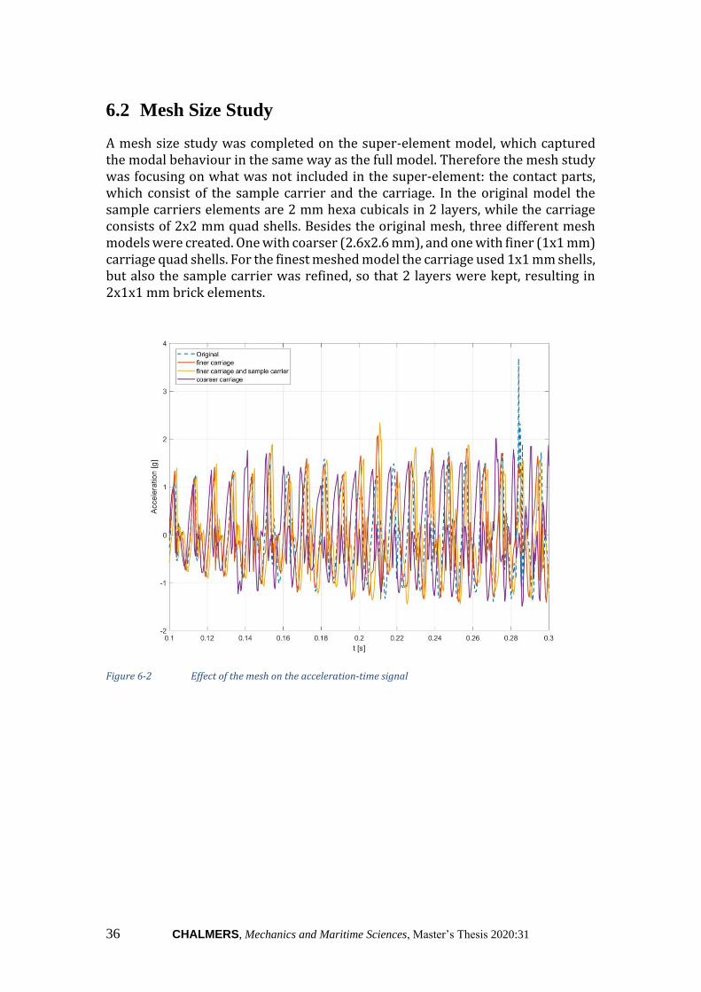
A mesh size study was completed on the super-element model, which captured the modal behaviour in the same way as the full model. Therefore the mesh study was focusing on what was not included in the super-element: the contact parts, which consist of the sample carrier and the carriage. In the original model the sample carriers elements are 2 mm hexa cubicals in 2 layers, while the carriage consists of 2x2 mm quad shells. Besides the original mesh, three different mesh models were created. One with coarser (2.6x2.6 mm), and one with finer (1x1 mm) carriage quad shells. For the finest meshed model the carriage used 1x1 mm shells, but also the sample carrier was refined, so that 2 layers were kept, resulting in 2x1x1 mm brick elements.
Figure 6-2 Effect of the mesh on the acceleration-time signal
CHALMERS, Mechanics and Maritime Sciences, Master’s Thesis 2020:31 37
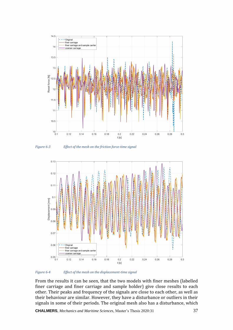
Figure 6-3 Effect of the mesh on the friction force-time signal
Figure 6-4 Effect of the mesh on the displacement-time signal
From the results it can be seen, that the two models with finer meshes (labelled finer carriage and finer carriage and sample holder) give close results to each other. Their peaks and frequency of the signals are close to each other, as well as their behaviour are similar. However, they have a disturbance or outliers in their signals in some of their periods. The original mesh also has a disturbance, which
38 CHALMERS, Mechanics and Maritime Sciences, Master’s Thesis 2020:31
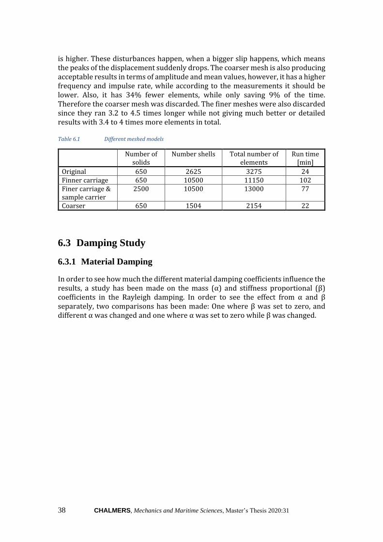
is higher. These disturbances happen, when a bigger slip happens, which means the peaks of the displacement suddenly drops. The coarser mesh is also producing acceptable results in terms of amplitude and mean values, however, it has a higher frequency and impulse rate, while according to the measurements it should be lower. Also, it has 34% fewer elements, while only saving 9% of the time. Therefore the coarser mesh was discarded. The finer meshes were also discarded since they ran 3.2 to 4.5 times longer while not giving much better or detailed results with 3.4 to 4 times more elements in total. Table 6.1 Different meshed models
Number of solids
Number shells Total number of elements
Run time [min]
Original 650 2625 3275 24 Finner carriage 650 10500 11150 102 Finer carriage & sample carrier
2500 10500 13000 77
Coarser 650 1504 2154 22
6.3 Damping Study
6.3.1 Material Damping
In order to see how much the different material damping coefficients influence the results, a study has been made on the mass (α) and stiffness proportional (β) coefficients in the Rayleigh damping. In order to see the effect from α and β separately, two comparisons has been made: One where β was set to zero, and different α was changed and one where α was set to zero while β was changed.
CHALMERS, Mechanics and Maritime Sciences, Master’s Thesis 2020:31 39
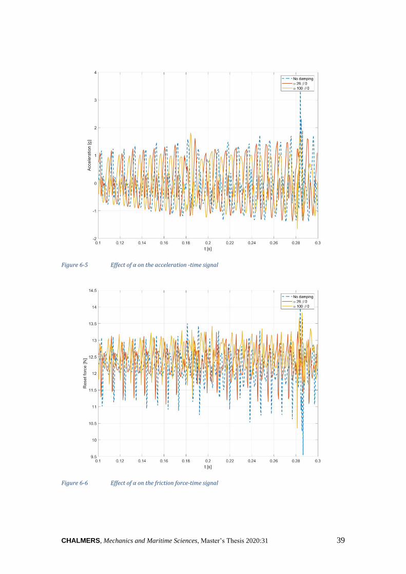
Figure 6-5 Effect of α on the acceleration -time signal
Figure 6-6 Effect of α on the friction force-time signal
40 CHALMERS, Mechanics and Maritime Sciences, Master’s Thesis 2020:31
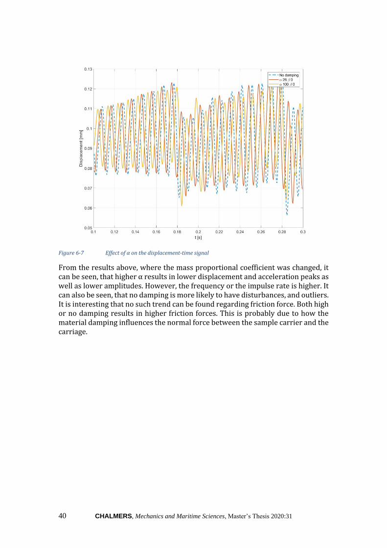
Figure 6-7 Effect of α on the displacement-time signal
From the results above, where the mass proportional coefficient was changed, it can be seen, that higher α results in lower displacement and acceleration peaks as well as lower amplitudes. However, the frequency or the impulse rate is higher. It can also be seen, that no damping is more likely to have disturbances, and outliers. It is interesting that no such trend can be found regarding friction force. Both high or no damping results in higher friction forces. This is probably due to how the material damping influences the normal force between the sample carrier and the carriage.
CHALMERS, Mechanics and Maritime Sciences, Master’s Thesis 2020:31 41
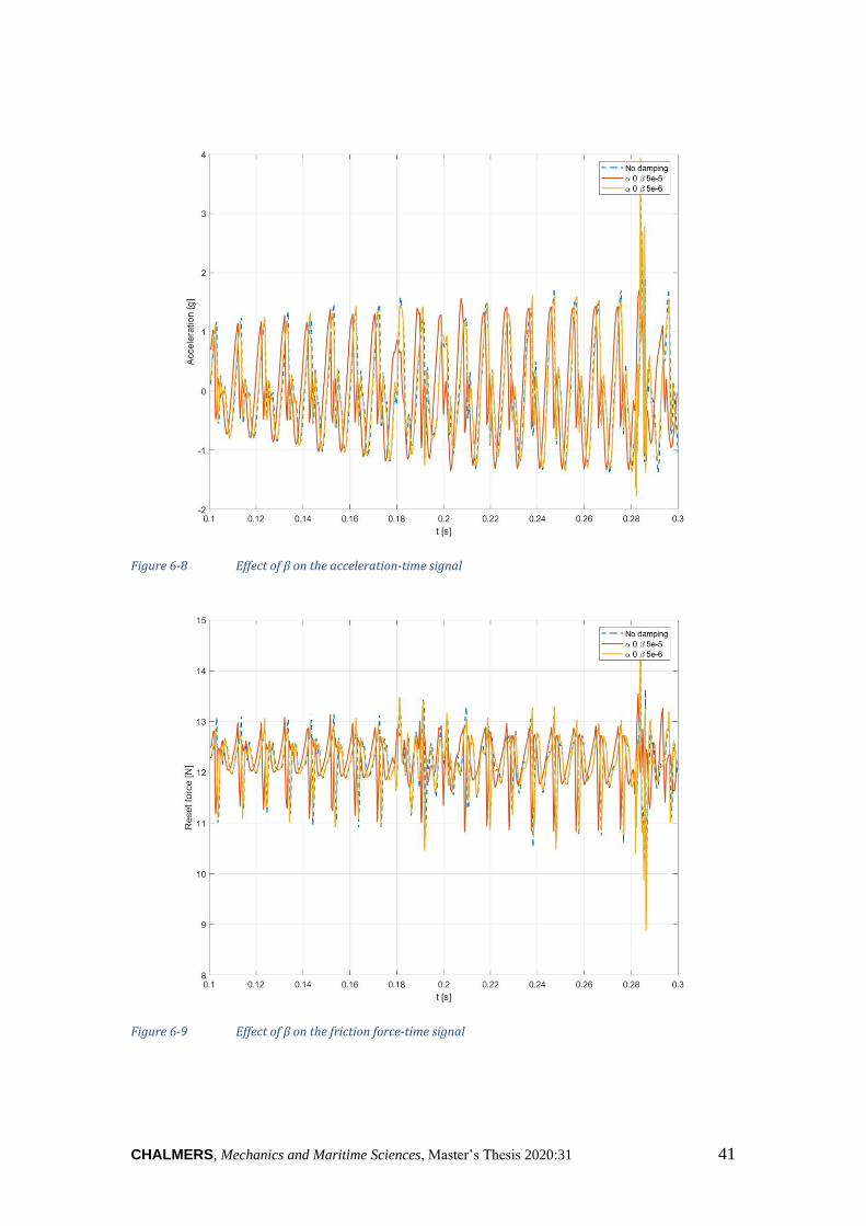
Figure 6-8 Effect of β on the acceleration-time signal
Figure 6-9 Effect of β on the friction force-time signal
42 CHALMERS, Mechanics and Maritime Sciences, Master’s Thesis 2020:31
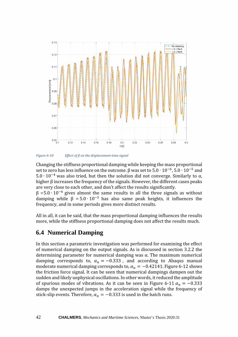
Figure 6-10 Effect of β on the displacement-time signal
Changing the stiffness proportional damping while keeping the mass proportional set to zero has less influence on the outcome. β was set to 5.0 ∙ 10−6, 5.0 ∙ 10−5 and 5.0 ∙ 10−4 was also tried, but then the solution did not converge. Similarly to α, higher β increases the frequency of the signals. However, the different cases peaks are very close to each other, and don’t affect the results significantly. β =5.0 ∙ 10−6 gives almost the same results in all the three signals as without damping while β = 5.0 ∙ 10−5 has also same peak heights, it influences the frequency, and in some periods gives more distinct results. All in all, it can be said, that the mass proportional damping influences the results more, while the stiffness proportional damping does not affect the results much.
6.4 Numerical Damping
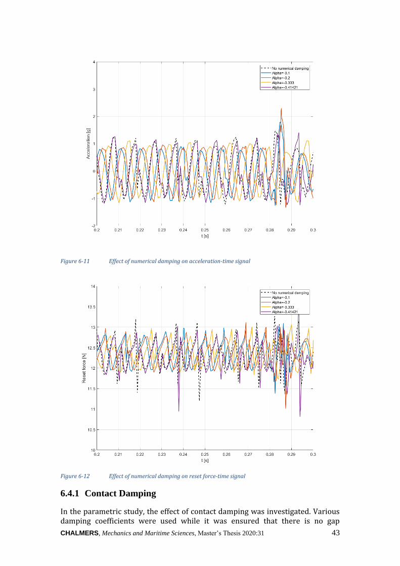
In this section a parametric investigation was performed for examining the effect of numerical damping on the output signals. As is discussed in section 3.2.2 the determining parameter for numerical damping was α. The maximum numerical damping corresponds to, 𝛼𝑛 = −0.333 , and according to Abaqus manual moderate numerical damping corresponds to, 𝛼𝑛 = −0.42141. Figure 6-12 shows the friction force signal. It can be seen that numerical dampings dampen out the sudden and likely unphysical oscillations. In other words, it reduced the amplitude of spurious modes of vibrations. As it can be seen in Figure 6-11 𝛼𝑛 = −0.333 damps the unexpected jumps in the acceleration signal while the frequency of stick-slip events. Therefore, 𝛼𝑛 = −0.333 is used in the batch runs.
CHALMERS, Mechanics and Maritime Sciences, Master’s Thesis 2020:31 43
Figure 6-11 Effect of numerical damping on acceleration-time signal
Figure 6-12 Effect of numerical damping on reset force-time signal
6.4.1 Contact Damping
In the parametric study, the effect of contact damping was investigated. Various damping coefficients were used while it was ensured that there is no gap
44 CHALMERS, Mechanics and Maritime Sciences, Master’s Thesis 2020:31
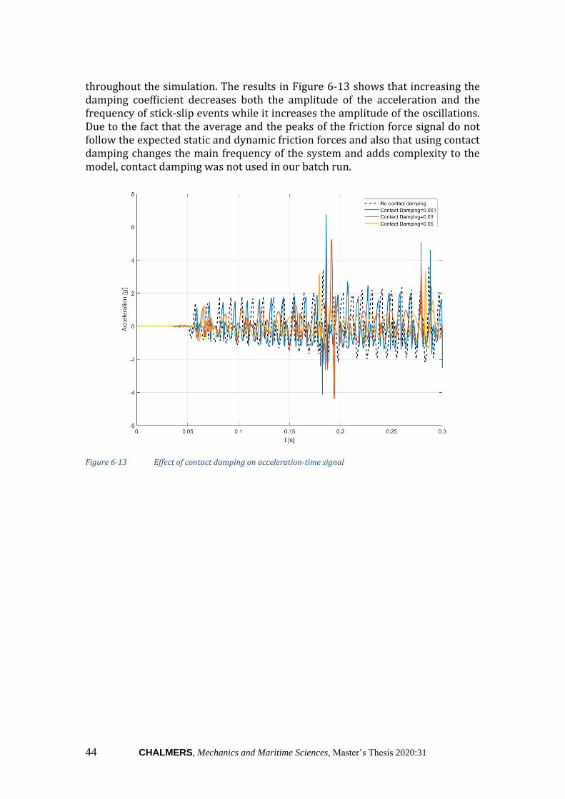
throughout the simulation. The results in Figure 6-13 shows that increasing the damping coefficient decreases both the amplitude of the acceleration and the frequency of stick-slip events while it increases the amplitude of the oscillations. Due to the fact that the average and the peaks of the friction force signal do not follow the expected static and dynamic friction forces and also that using contact damping changes the main frequency of the system and adds complexity to the model, contact damping was not used in our batch run.
Figure 6-13 Effect of contact damping on acceleration-time signal
CHALMERS, Mechanics and Maritime Sciences, Master’s Thesis 2020:31 45
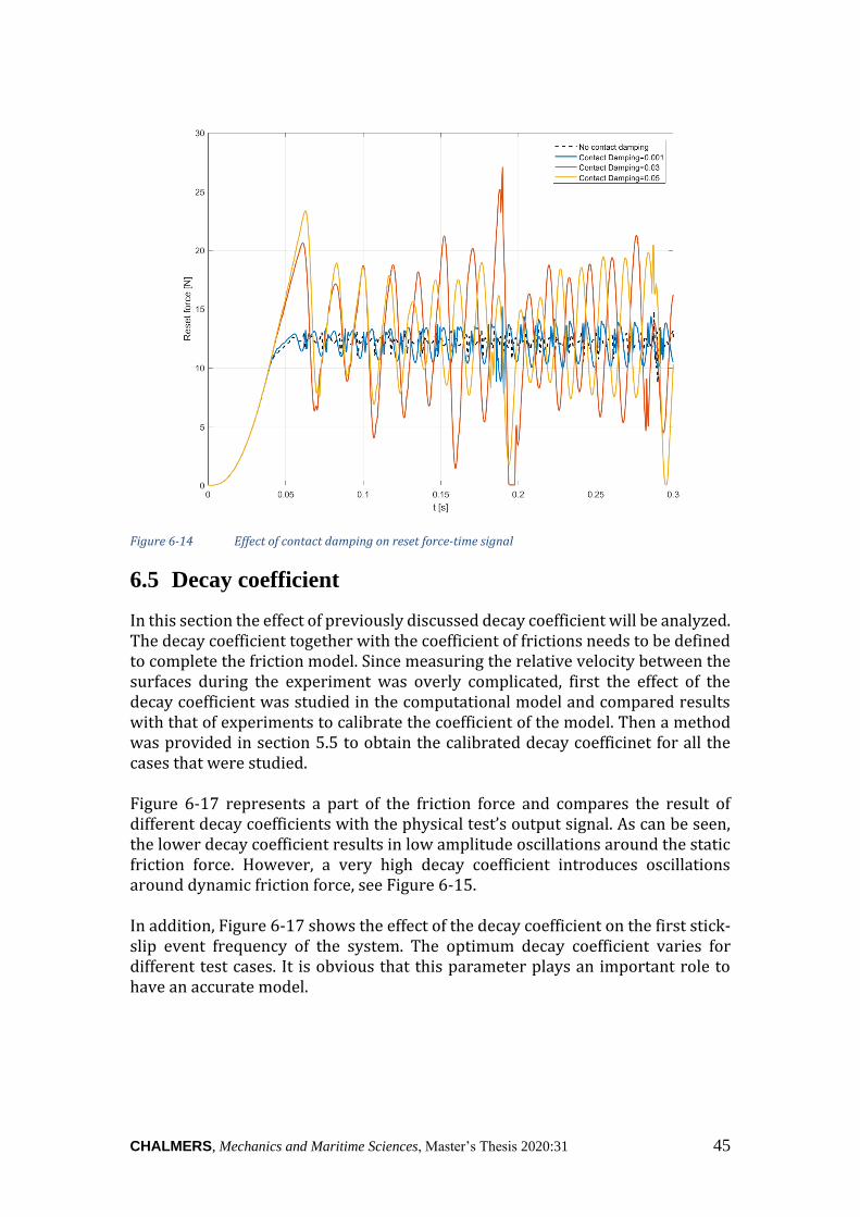
Figure 6-14 Effect of contact damping on reset force-time signal
6.5 Decay coefficient
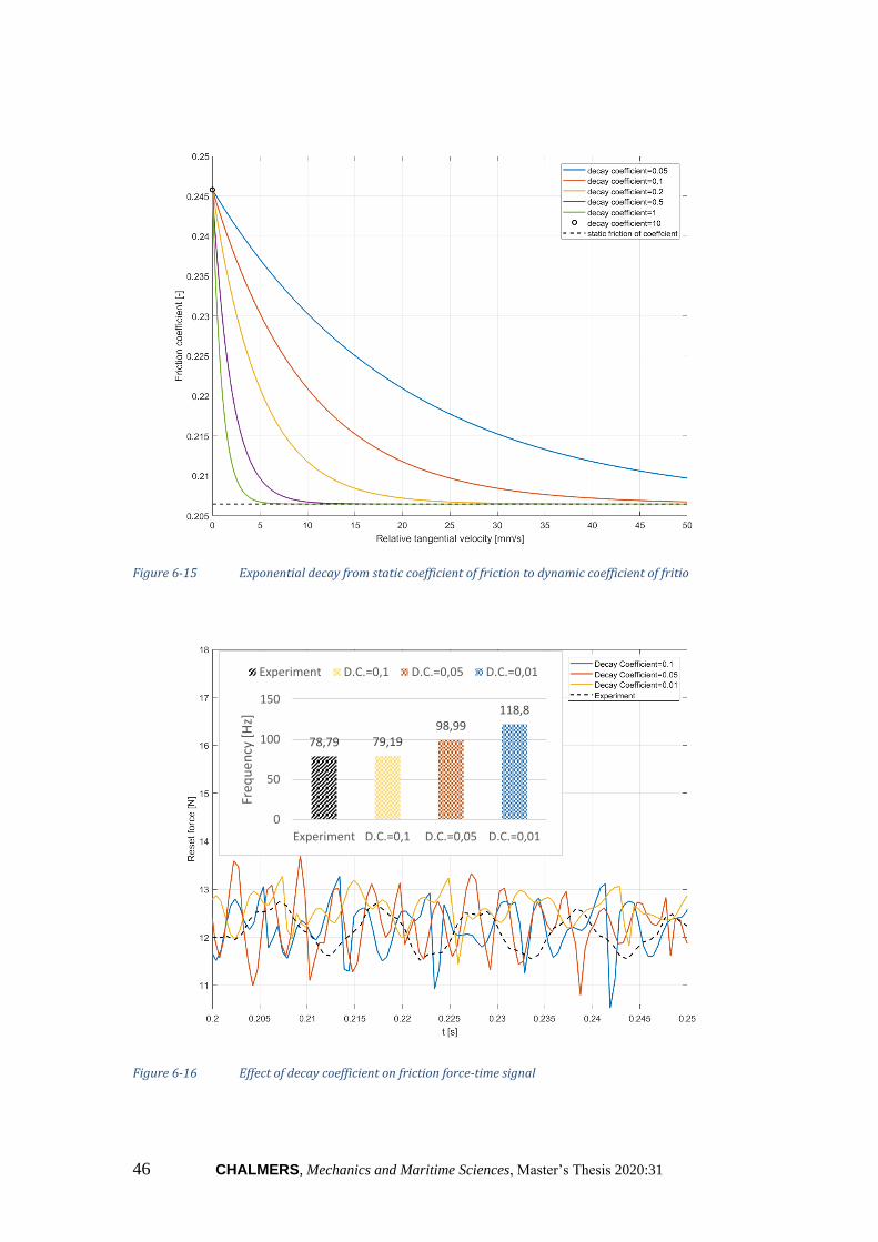
In this section the effect of previously discussed decay coefficient will be analyzed. The decay coefficient together with the coefficient of frictions needs to be defined to complete the friction model. Since measuring the relative velocity between the surfaces during the experiment was overly complicated, first the effect of the decay coefficient was studied in the computational model and compared results with that of experiments to calibrate the coefficient of the model. Then a method was provided in section 5.5 to obtain the calibrated decay coefficinet for all the cases that were studied. Figure 6-17 represents a part of the friction force and compares the result of different decay coefficients with the physical test’s output signal. As can be seen, the lower decay coefficient results in low amplitude oscillations around the static friction force. However, a very high decay coefficient introduces oscillations around dynamic friction force, see Figure 6-15. In addition, Figure 6-17 shows the effect of the decay coefficient on the first stick-slip event frequency of the system. The optimum decay coefficient varies for different test cases. It is obvious that this parameter plays an important role to have an accurate model.
46 CHALMERS, Mechanics and Maritime Sciences, Master’s Thesis 2020:31
Figure 6-15 Exponential decay from static coefficient of friction to dynamic coefficient of fritio
Figure 6-17 Effect of decay coefficient on friction force-time signal
78,79 79,1998,99
118,8
0
50
100
150
Experiment D.C.=0,1 D.C.=0,05 D.C.=0,01
Freq
uen
cy [
Hz]
Experiment D.C.=0,1 D.C.=0,05 D.C.=0,01
Figure 6-16 Effect of decay coefficient on friction force-time signal
CHALMERS, Mechanics and Maritime Sciences, Master’s Thesis 2020:31 47
6.6 Elastic slip
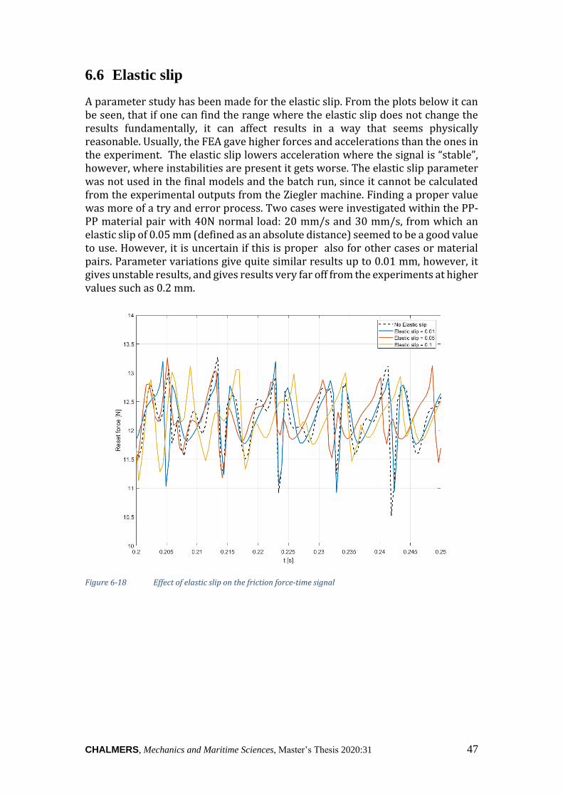
A parameter study has been made for the elastic slip. From the plots below it can be seen, that if one can find the range where the elastic slip does not change the results fundamentally, it can affect results in a way that seems physically reasonable. Usually, the FEA gave higher forces and accelerations than the ones in the experiment. The elastic slip lowers acceleration where the signal is “stable”, however, where instabilities are present it gets worse. The elastic slip parameter was not used in the final models and the batch run, since it cannot be calculated from the experimental outputs from the Ziegler machine. Finding a proper value was more of a try and error process. Two cases were investigated within the PP-PP material pair with 40N normal load: 20 mm/s and 30 mm/s, from which an elastic slip of 0.05 mm (defined as an absolute distance) seemed to be a good value to use. However, it is uncertain if this is proper also for other cases or material pairs. Parameter variations give quite similar results up to 0.01 mm, however, it gives unstable results, and gives results very far off from the experiments at higher values such as 0.2 mm.
Figure 6-18 Effect of elastic slip on the friction force-time signal
48 CHALMERS, Mechanics and Maritime Sciences, Master’s Thesis 2020:31
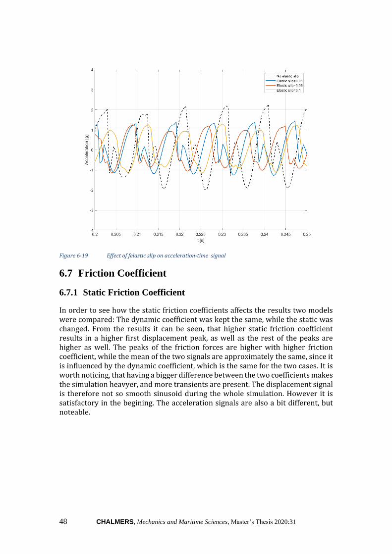
Figure 6-19 Effect of felastic slip on acceleration-time signal
6.7 Friction Coefficient
6.7.1 Static Friction Coefficient
In order to see how the static friction coefficients affects the results two models were compared: The dynamic coefficient was kept the same, while the static was changed. From the results it can be seen, that higher static friction coefficient results in a higher first displacement peak, as well as the rest of the peaks are higher as well. The peaks of the friction forces are higher with higher friction coefficient, while the mean of the two signals are approximately the same, since it is influenced by the dynamic coefficient, which is the same for the two cases. It is worth noticing, that having a bigger difference between the two coefficients makes the simulation heavyer, and more transients are present. The displacement signal is therefore not so smooth sinusoid during the whole simulation. However it is satisfactory in the begining. The acceleration signals are also a bit different, but noteable.
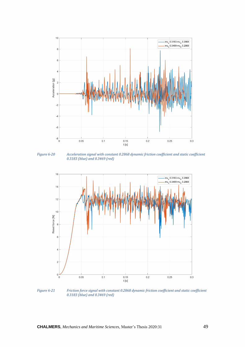
CHALMERS, Mechanics and Maritime Sciences, Master’s Thesis 2020:31 49
Figure 6-20 Acceleration signal with constant 0.2868 dynamic friction coefficient and static coefficient
0.3183 (blue) and 0.3469 (red)
Figure 6-21 Friction force signal with constant 0.2868 dynamic friction coefficient and static coefficient
0.3183 (blue) and 0.3469 (red)
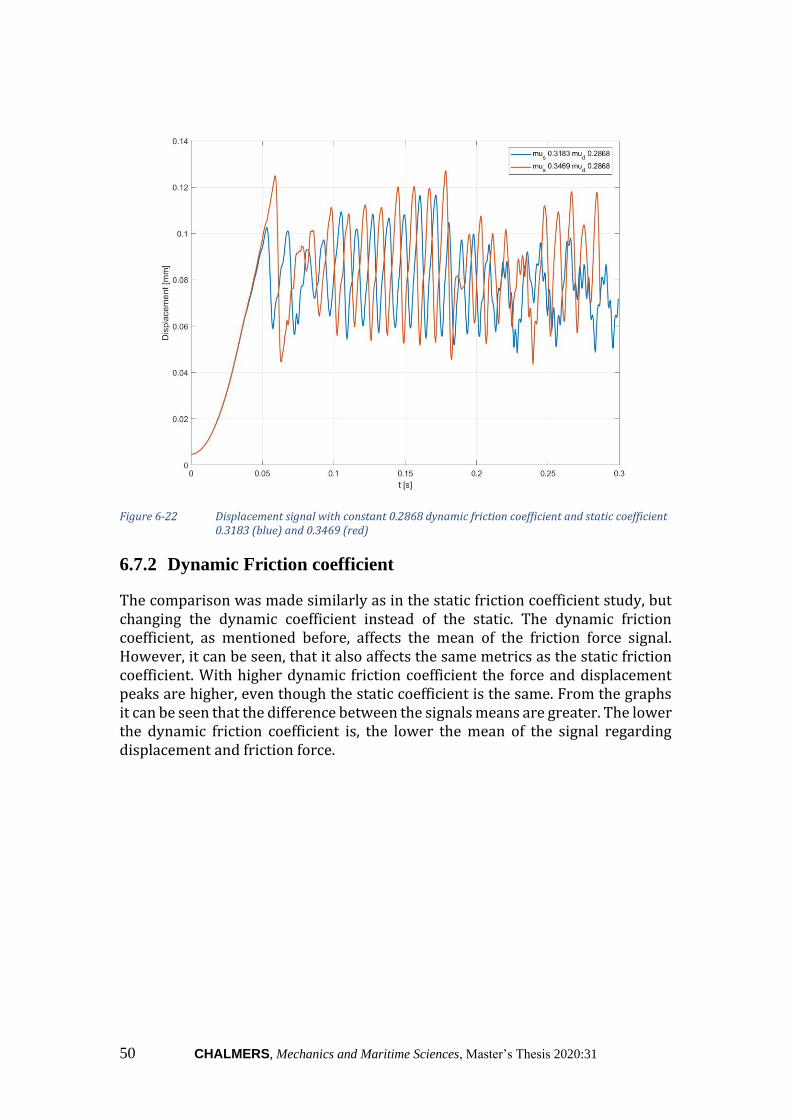
50 CHALMERS, Mechanics and Maritime Sciences, Master’s Thesis 2020:31
Figure 6-22 Displacement signal with constant 0.2868 dynamic friction coefficient and static coefficient
0.3183 (blue) and 0.3469 (red)
6.7.2 Dynamic Friction coefficient
The comparison was made similarly as in the static friction coefficient study, but changing the dynamic coefficient instead of the static. The dynamic friction coefficient, as mentioned before, affects the mean of the friction force signal. However, it can be seen, that it also affects the same metrics as the static friction coefficient. With higher dynamic friction coefficient the force and displacement peaks are higher, even though the static coefficient is the same. From the graphs it can be seen that the difference between the signals means are greater. The lower the dynamic friction coefficient is, the lower the mean of the signal regarding displacement and friction force.
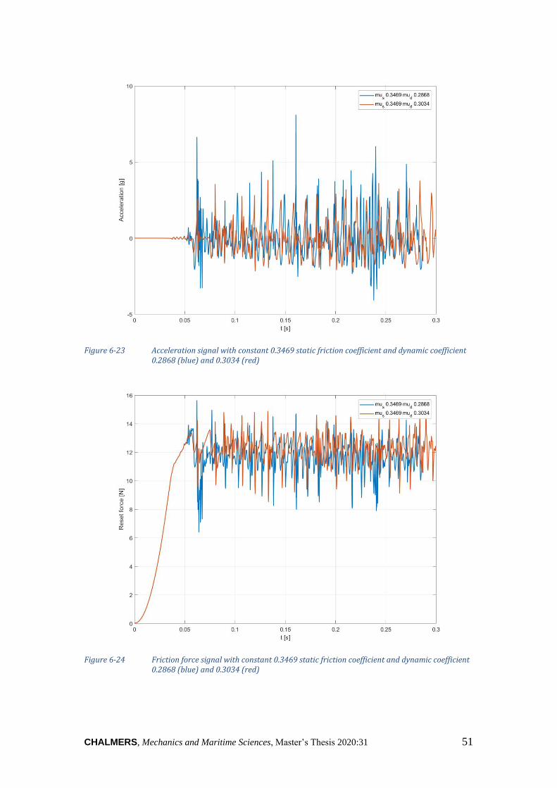
CHALMERS, Mechanics and Maritime Sciences, Master’s Thesis 2020:31 51
Figure 6-23 Acceleration signal with constant 0.3469 static friction coefficient and dynamic coefficient
0.2868 (blue) and 0.3034 (red)
Figure 6-24 Friction force signal with constant 0.3469 static friction coefficient and dynamic coefficient
0.2868 (blue) and 0.3034 (red)
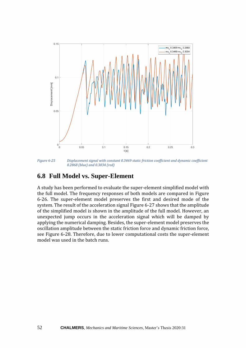
52 CHALMERS, Mechanics and Maritime Sciences, Master’s Thesis 2020:31
Figure 6-25 Displacement signal with constant 0.3469 static friction coefficient and dynamic coefficient
0.2868 (blue) and 0.3034 (red)
6.8 Full Model vs. Super-Element
A study has been performed to evaluate the super-element simplified model with the full model. The frequency responses of both models are compared in Figure 6-26. The super-element model preserves the first and desired mode of the system. The result of the acceleration signal Figure 6-27 shows that the amplitude of the simplified model is shown in the amplitude of the full model. However, an unexpected jump occurs in the acceleration signal which will be damped by applying the numerical damping. Besides, the super-element model preserves the oscillation amplitude between the static friction force and dynamic friction force, see Figure 6-28. Therefore, due to lower computational costs the super-element model was used in the batch runs.
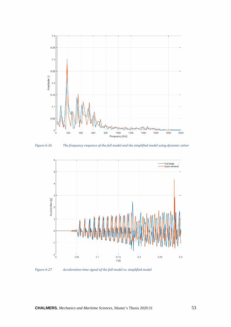
CHALMERS, Mechanics and Maritime Sciences, Master’s Thesis 2020:31 53
Figure 6-26 The frequency responce of the full model and the simplified model using dynamic solver
Figure 6-27 Acceleration-time signal of the full model vs. simplified model
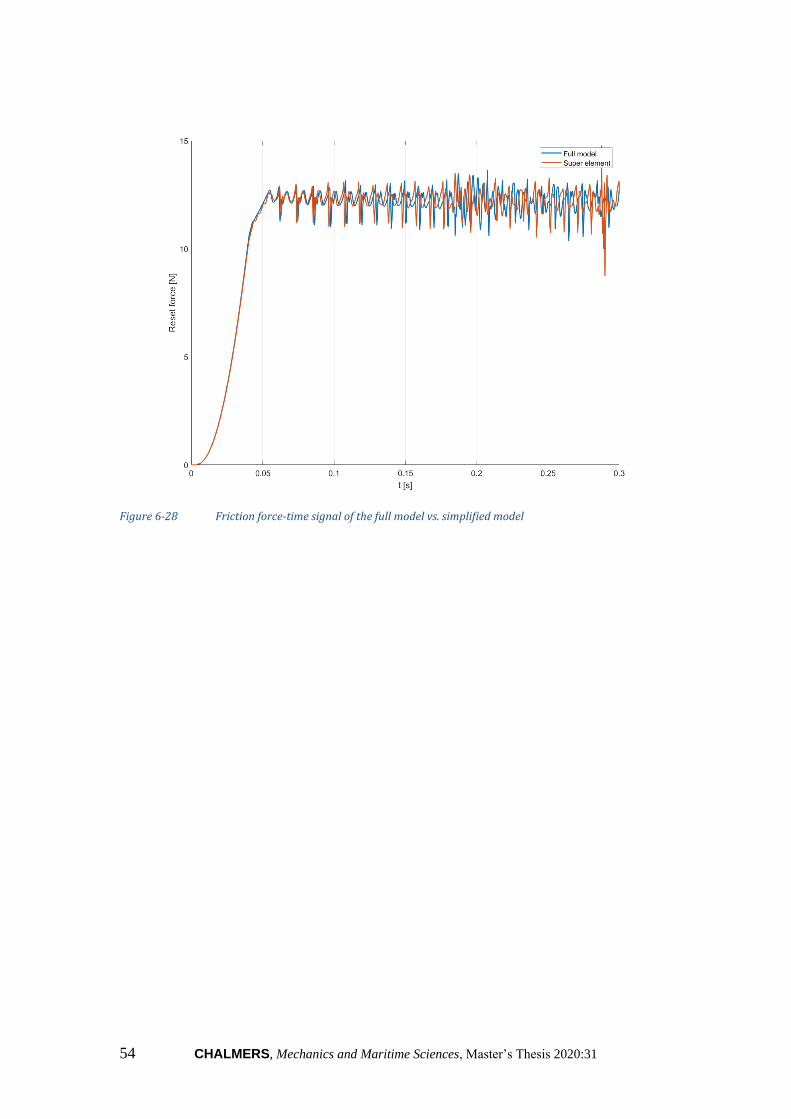
54 CHALMERS, Mechanics and Maritime Sciences, Master’s Thesis 2020:31
Figure 6-28 Friction force-time signal of the full model vs. simplified model

CHALMERS, Mechanics and Maritime Sciences, Master’s Thesis 2020:31 55
7 Results and discussions
7.1 Postprocessing of Output Signals
In order to be able to compare the FEA results to the experimental ones, some metrics had to be established. The experimental setup calculated some of the metrics, like impulse rate, for the whole signal, which contained usually 3 cycles see Figure 5-4. However, FEM was used only to simulate a short duration of it from which the friction coefficients were calculated described in section 5.4. Also, only in the last 0.1 second of the simulation the carriage moved with the predescribed speed. Therefore only that part of the FE output was compared with the experiment. In order to compare similar signals the following assessment was made.
7.1.1 Selecting Signal Parts
A 0.05 s long signal was selected in the FEM output, with as few judged outliers as possible. Having a longer signal would have resulted with more disturbances, which would have affected some metrics regarding acceleration. The start and end times were selected manually for FE and experimental cases. The selection was done so, that either the start time was just before a cycles peak, or the end time after a cycles peak in the FE model. It was found preferable to try to find a good end point, and just use the 0.05 s long part before, since experiments postprocessing was done this way. The start and end times were the same for all the signals in the FE model, except the velocity, where a longer time signal was selected in order to calculate the impulse rate more accurately. The measurement outputs only consist of two signals: the acceleration and the friction force time signals. The experimental output was easy to handle, since it was almost perfectly periodic and easy to handle in many aspects. Peak and cycle finding was simple, and all the periods were very similar. Therefore the analysing procedure was easy to automate. Since the time periods selected for comparisons are short therefore not many periods fits within the time frame. Usually 5-7 periods fit within 0.05 s long signal. It is important for the compared signals to either start or end in the same phase, so that the impulse rate gives better correlation. The selected experimental friction force signal was 0.1 s long even though the FE signal was only 0.05 s long. The unimportance of having the same signal length, and having an 0.1 s long signal from the experiments regarding friction force is due to two facts: First, that only impulse rate, mean of signal, and mean of the peaks are outputted from the experimental data. Furthermore, the mean of the signal, and the mean of peaks are not influenced by the length of time selected. Secondly, the 0.1 s gives more accurate number regarding impulse rate, since more cycles are captured in a longer time, which gives smaller error. The length of FE was not longer than 0.05 s in order to capture exactly the same time period captured in the accelerations.
56 CHALMERS, Mechanics and Maritime Sciences, Master’s Thesis 2020:31
The impulse rate, as mentioned before, was calculated from an 0.1 s long signal from the friction force in experiments. However, in FE, the impulse rate was calculated from the velocity signal, since it was much smoother than the rapidly fluctuating acceleration and friction force signals. The velocity, displacement and acceleration signals had the same frequency, therefore the impulse rate could have been calculated from all of them. Due to practical reasons it was decided to calculate it from the velocity signal, since they were easier to handle an automatize in Matlab. The velocity signals other metrics were also calculated from this signal. Since these metrics were not so important, it was not necessary to have exactly the same time periods as selected manually for FE. The displacement was captured by the user defined 0.05 second long time frame in FE.
7.1.2 Metrics compared
Although many other metrics were investigated and correlated, this work only discusses the following metrics: From the acceleration signals both in experiment and CAE the following metrics were calculated:
1. The maximum of the signal 2. The mean of the peaks. The peaks from the FE output had to be checked
manually, in order to find one or maximum two peaks for one cycle. Friction force signals:
1. Mean of the signal for both CAE and experiment, which corresponds to the dynamic friction force.
2. Mean of the peaks for both CAE and experimental outputs. This value corresponds to the static friction force.
3. Maximum of experimental output. This value was usually very close to the mean of the signals peaks, since the maximum value was not an outlying data. The maximum in CAE was not outputted since in most of the cases it was an outlying data with no valuable information, therefore it was considered not to be representative.
4. Impulse rate from the experimental data. As mentioned before the CAE outputs impulse rate was calculated from the velocity output.
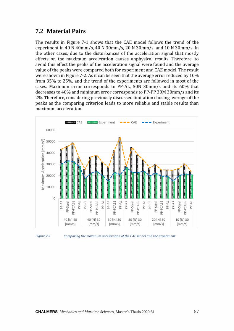
CHALMERS, Mechanics and Maritime Sciences, Master’s Thesis 2020:31 57
7.2 Material Pairs
The results in Figure 7-1 shows that the CAE model follows the trend of the experiment in 40 N 40mm/s, 40 N 30mm/s, 20 N 30mm/s and 10 N 30mm/s. In the other cases, due to the disturbances of the acceleration signal that mostly effects on the maximum acceleration causes unphysical results. Therefore, to avoid this effect the peaks of the acceleration signal were found and the average value of the peaks were compared both for experiment and CAE model. The result were shown in Figure 7-2. As it can be seen that the average error reduced by 10% from 35% to 25%, and the trend of the experiments are followed in most of the cases. Maximum error corresponds to PP-AL, 50N 30mm/s and its 60% that decreases to 40% and minimum error corresponds to PP-PP 30M 30mm/s and its 2%. Therefore, considering previously discussed limitation chosing average of the peaks as the comparing criterion leads to more reliable and stable results than maximum acceleration.
Figure 7-1 Comparing the maximum acceleration of the CAE model and the experiment
0
10000
20000
30000
40000
50000
60000
PP
-PP
PP
-Ste
el
PP
-PC
AB
S
PP
-AL
PP
-PP
PP
-Ste
el
PP
-PC
AB
S
PP
-AL
PP
-PP
PP
-PC
AB
S
PP
-AL
PP
-PP
PP
-Ste
el
PP
-PC
AB
S
PP
-AL
PP
-PP
PP
-Ste
el
PP
-PC
AB
S
PP
-AL
PP
-PP
PP
-Ste
el
PP
-PC
AB
S
PP
-AL
40 [N] 40[mm/s]
40 [N] 30[mm/s]
50 [N] 30[mm/s]
30 [N] 30[mm/s]
20 [N] 30[mm/s]
10 [N] 30[mm/s]
Max
imu
m A
ccel
erat
ion
[m
m/s
2]
CAE Experiment CAE Experiment
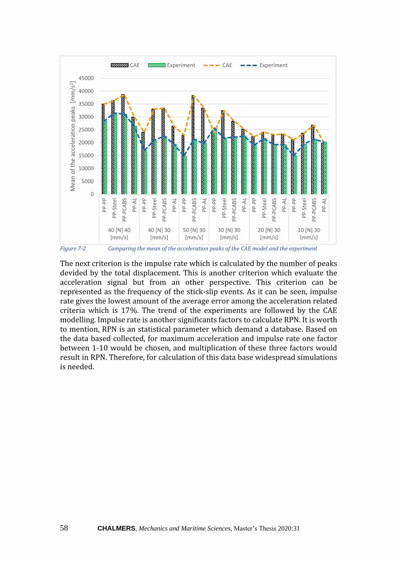
58 CHALMERS, Mechanics and Maritime Sciences, Master’s Thesis 2020:31
Figure 7-2 Comparing the mean of the acceleration peaks of the CAE model and the experiment
The next criterion is the impulse rate which is calculated by the number of peaks devided by the total displacement. This is another criterion which evaluate the acceleration signal but from an other perspective. This criterion can be represented as the frequency of the stick-slip events. As it can be seen, impulse rate gives the lowest amount of the average error among the acceleration related criteria which is 17%. The trend of the experiments are followed by the CAE modelling. Impulse rate is another significants factors to calculate RPN. It is worth to mention, RPN is an statistical parameter which demand a database. Based on the data based collected, for maximum acceleration and impulse rate one factor between 1-10 would be chosen, and multiplication of these three factors would result in RPN. Therefore, for calculation of this data base widespread simulations is needed.
0
5000
10000
15000
20000
25000
30000
35000
40000
45000
PP
-PP
PP
-Ste
el
PP
-PC
AB
S
PP
-AL
PP
-PP
PP
-Ste
el
PP
-PC
AB
S
PP
-AL
PP
-PP
PP
-PC
AB
S
PP
-AL
PP
-PP
PP
-Ste
el
PP
-PC
AB
S
PP
-AL
PP
-PP
PP
-Ste
el
PP
-PC
AB
S
PP
-AL
PP
-PP
PP
-Ste
el
PP
-PC
AB
S
PP
-AL
40 [N] 40[mm/s]
40 [N] 30[mm/s]
50 [N] 30[mm/s]
30 [N] 30[mm/s]
20 [N] 30[mm/s]
10 [N] 30[mm/s]
Mea
n o
f th
e ac
cele
rati
on
pea
ks [
mm
/s2]
CAE Experiment CAE Experiment
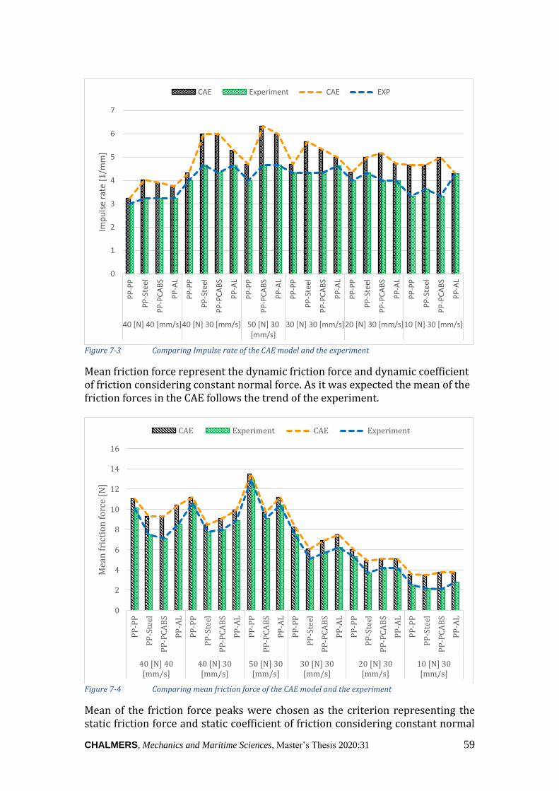
CHALMERS, Mechanics and Maritime Sciences, Master’s Thesis 2020:31 59
Figure 7-3 Comparing Impulse rate of the CAE model and the experiment
Mean friction force represent the dynamic friction force and dynamic coefficient of friction considering constant normal force. As it was expected the mean of the friction forces in the CAE follows the trend of the experiment.
Figure 7-4 Comparing mean friction force of the CAE model and the experiment
Mean of the friction force peaks were chosen as the criterion representing the static friction force and static coefficient of friction considering constant normal
0
1
2
3
4
5
6
7
PP
-PP
PP
-Ste
el
PP
-PC
AB
S
PP
-AL
PP
-PP
PP
-Ste
el
PP
-PC
AB
S
PP
-AL
PP
-PP
PP
-PC
AB
S
PP
-AL
PP
-PP
PP
-Ste
el
PP
-PC
AB
S
PP
-AL
PP
-PP
PP
-Ste
el
PP
-PC
AB
S
PP
-AL
PP
-PP
PP
-Ste
el
PP
-PC
AB
S
PP
-AL
40 [N] 40 [mm/s]40 [N] 30 [mm/s] 50 [N] 30[mm/s]
30 [N] 30 [mm/s]20 [N] 30 [mm/s]10 [N] 30 [mm/s]
Imp
uls
e ra
te [
1/m
m]
CAE Experiment CAE EXP
0
2
4
6
8
10
12
14
16
PP
-PP
PP
-Ste
el
PP
-PC
AB
S
PP
-AL
PP
-PP
PP
-Ste
el
PP
-PC
AB
S
PP
-AL
PP
-PP
PP
-PC
AB
S
PP
-AL
PP
-PP
PP
-Ste
el
PP
-PC
AB
S
PP
-AL
PP
-PP
PP
-Ste
el
PP
-PC
AB
S
PP
-AL
PP
-PP
PP
-Ste
el
PP
-PC
AB
S
PP
-AL
40 [N] 40[mm/s]
40 [N] 30[mm/s]
50 [N] 30[mm/s]
30 [N] 30[mm/s]
20 [N] 30[mm/s]
10 [N] 30[mm/s]
Mea
n f
rict
ion
fo
rce
[N]
CAE Experiment CAE Experiment
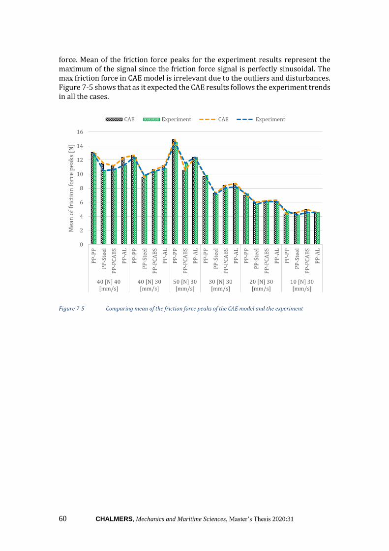
60 CHALMERS, Mechanics and Maritime Sciences, Master’s Thesis 2020:31
force. Mean of the friction force peaks for the experiment results represent the maximum of the signal since the friction force signal is perfectly sinusoidal. The max friction force in CAE model is irrelevant due to the outliers and disturbances. Figure 7-5 shows that as it expected the CAE results follows the experiment trends in all the cases.
Figure 7-5 Comparing mean of the friction force peaks of the CAE model and the experiment
0
2
4
6
8
10
12
14
16
PP
-PP
PP
-Ste
el
PP
-PC
AB
S
PP
-AL
PP
-PP
PP
-Ste
el
PP
-PC
AB
S
PP
-AL
PP
-PP
PP
-PC
AB
S
PP
-AL
PP
-PP
PP
-Ste
el
PP
-PC
AB
S
PP
-AL
PP
-PP
PP
-Ste
el
PP
-PC
AB
S
PP
-AL
PP
-PP
PP
-Ste
el
PP
-PC
AB
S
PP
-AL
40 [N] 40[mm/s]
40 [N] 30[mm/s]
50 [N] 30[mm/s]
30 [N] 30[mm/s]
20 [N] 30[mm/s]
10 [N] 30[mm/s]
Mea
n o
f fr
icti
on
fo
rce
pea
ks
[N]
CAE Experiment CAE Experiment
CHALMERS, Mechanics and Maritime Sciences, Master’s Thesis 2020:31 61
8 Conclusion
The FEA results capture well the trends experienced from experiments. Usually, the metrics show higher values for the FEA results. This is acceptable, since this thesis focuses on predicting squeak noise and the stick-slick phenomenon in CAE environment rather than capturing it precisely. Obviously, the parameters and methods can be further fine-tuned and studied to reach better correlation, however, the results are satisfactory here. Especially, since the goal is to have a robust model, which works well for different materials, normal forces, and velocities. By having higher values for the metrics in the FEA it overestimates the severity of the stick-slip events thus giving a conservative method of modelling the phenomenon. The bottleneck of the established method hides in the postprocessing of the signals. The FEA cannot simulate the whole experimental signal but only a selected preferably periodic part of it. Even though the postprocessing was automated as much as possible, engineering instinct is still needed when it comes to postprocessing as well as defining certain input parameters for the FEA. All in all, the results are promising, and hopefully the method developed for simulating stick-slip will be implemented in a framework in the early phases of product development.
8.1 Future work
While working on the project, many ideas and issues came up which this work unfortunately did not have time to investigate further. In the following section possible future works are listed worth considering: The parameter sensitivity analysis was mainly done on one material pair (PP-PP) with the velocity of 20 mm/s and 40 N normal force. Although some parameter study was carried out on the same model, but with 30 mm/s velocity, the sensitivity analysis might behave differently for other cases where either or both velocity and normal force is further from the tested values. Also, the parameters in the sensitivity analysis were changed individually, therefore it is unknown how much one parameter could affect another. Furthermore there are some parameters which was not implemented in the model, for example the elastic slip. Therefore one way to continue this work could be to investigate the FEM further. However, good results were achieved at the end of the thesis, and it is more recommended and important to continue to set up a framework with guidelines which can be implemented in the product development process.
62 CHALMERS, Mechanics and Maritime Sciences, Master’s Thesis 2020:31
9 References
1. Szekely, A.P. and N.A. Hanna, Nonlinear Modeling and Simulation of Impact Events and Validation with Experimental Tests. 2018, KTH Royal Institute of Technology School of Engineering Sciences: Stockholm.
2. Weber, J. and I. Benhayoun, Squeak & Rattle Correlation in Time Domain using the SAR-LINE™ Method. SAE International Journal of Passenger Cars-Mechanical Systems, 2012. 5(2012-01-1553): p. 1124-1132.
3. Zins. SSP-04 Stick-Slip Test Bench. 2016 June. 4. Zuleeg, J., How to measure, prevent, and eliminate stick-slip and noise
generation with lubricants. 2015, SAE Technical Paper. 5. Wriggers, P., Computational Contact Mechanics, Springer-Verlag. Berlin,
Heidelberg, 2006: p. 69-75, 76-80. 6. Best Practices for Contact Modeling for Accuracy and Accelerated
Convergence, in Science in the Age of Experience Conference. 2016. 7. Systemes, D., Abaqus 2016 Online documentation, D. Systemes, Editor.
2015. 8. Carlberg, J. and B. Toyib, Finite Element Modelling of Interlaminar Slip in
Stress-Laminated Timber Decks, Friction Interaction Modelling Using Abaqus. 2012.
9. Hans, S., et al., Damping identification in multi-degree-of-freedom system via a wavelet-logarithmic decrement—part 2: study of a civil engineering building. Journal of Sound and Vibration, 2000. 235(3): p. 375-403.
10. Shi, X. and A.A. Polycarpou, Measurement and modeling of normal contact stiffness and contact damping at the meso scale. J. Vib. Acoust., 2005. 127(1): p. 52-60.
11. de Klerk, D., D.J. Rixen, and S. Voormeeren, General framework for dynamic substructuring: history, review and classification of techniques. AIAA journal, 2008. 46(5): p. 1169-1181.
12. Voormeeren, S.N., Dynamic substructuring methodologies for integrated dynamic analysis of wind turbines. 2012.
13. Godborg, F. and A. Valiyakath Basheer, Model reduction of finite element models applied to nonlinear squeak and rattle simulation. 2019.
14. Holzwarth, P. and P. Eberhard, Interface reduction for CMS methods and alternative model order reduction. IFAC-PapersOnLine, 2015. 48(1): p. 254-259.
15. Guyan, R.J., Reduction of stiffness and mass matrices. AIAA journal, 1965. 3(2): p. 380-380.
16. Systèmes, D., SIMULIA User Assistance 2017. Abaqus Documentation: Providence, RI, USA, 2017.
17. Lundgren, V., Stick-Slip Friction in Polymer-Polymer Contacts: A Comparison of Two Test Methods. 2016.


DEPARTMENT OF Mechanics and Maritime
Sciences
CHALMERS UNIVERSITY OF TECHNOLOGY
Gothenburg, Sweden
www.chalmers.se