simulation study of solar wind push on a charged wire...

Ann. Geophys., 25, 755–767, 2007www.ann-geophys.net/25/755/2007/© European Geosciences Union 2007

AnnalesGeophysicae

Simulation study of solar wind push on a charged wire: basis ofsolar wind electric sail propulsion

P. Janhunen1,2 and A. Sandroos2

1University of Helsinki, Department of Physical Sciences, Finland2Finnish Meteorological Institute, Space Research, Finland

Received: 11 May 2006 – Revised: 20 February 2007 – Accepted: 1 March 2007 – Published: 29 March 2007

Abstract. One possibility for propellantless propulsion inspace is to use the momentum flux of the solar wind. A wayto set up a solar wind sail is to have a set of thin long wireswhich are kept at high positive potential by an onboard elec-tron gun so that the wires repel and deflect incident solarwind protons. The efficiency of this so-called electric saildepends on how large force a given solar wind exerts on awire segment and how large electron current the wire seg-ment draws from the solar wind plasma when kept at a givenpotential. We use 1-D and 2-D electrostatic plasma simu-lations to calculate the force and present a semitheoreticalformula which captures the simulation results. We find thatunder average solar wind conditions at 1 AU the force perunit length is (5±1)×10−8 N/m for 15 kV potential and thatthe electron current is accurately given by the well-knownorbital motion limited (OML) theory cylindrical Langmuirprobe formula. Although the force may appear small, ananalysis shows that because of the very low weight of a thinwire per unit length, quite high final speeds (over 50 km/s)could be achieved by an electric sailing spacecraft using to-day’s flight-proved components. It is possible that artificialelectron heating of the plasma in the interaction region couldincrease the propulsive effect even further.

Keywords. General or miscellaneous (Instruments useful inthree or more fields; New fields (not classifiable under otherheadings); Techniques applicable in three or more fields)

1 Introduction

The level of used propulsion technology is the decisive fac-tor which ultimately sets the scale and scope of human spaceactivity. Besides traditional chemical rockets which canbe used both inside and outside of planetary atmospheres,

Correspondence to:P. Janhunen([email protected])

space-only propulsion techniques such as electric propulsion(ion and plasma engines) and solar sails have gained popu-larity in recent years. Both mentioned techniques have beenin principle known for a long time. Likewise, there is muchresearch going on in terms of really advanced (and at thesame time long-term) propulsion concepts using e.g. fusionreactors, laser sails or antimatter, with the ultimate goal ofenabling interstellar travel.

In this paper we consider a near-term propellantless spacephysics based sailing method which uses the solar wind mo-mentum flux, i.e. the solar wind dynamic pressurePdyn=ρv2

which is on the average about 2 nPa at 1 AU distance fromthe Sun. The idea of using solar wind momentum was firstconsidered byZubrin and Andrews(1991) who suggestedcreating an artificial magnetosphere around the spacecraft todeflect the solar wind and thus extract momentum from it.As an alternative way of tapping solar wind momentum theelectric sail was suggested byJanhunen(2004). The electricsail consists of a number of long and thin conductive wires ortethers which are kept at a positive potential with the help ofan onboard electron gun (one could also consider a negativeion gun, this variant is not pursued in this paper however). In-vestigating the interaction of the solar wind around a singlecharged wire and predicting the obtained thrust in differentsolar wind conditions and different wire potentials is the taskof the present paper.

2 Theory

Consider a long positively charged wire placed in solar windwhich blows perpendicular to it to the x-direction. To calcu-late the force acting on the wire, it is sufficient to know thepotential pattern because from that one can easily computethe solar wind proton trajectories numerically. For each inci-dent proton its deflection angle tells how much x-directedmomentum the particle has lost in its interaction with the

Published by Copernicus GmbH on behalf of the European Geosciences Union.

756 P. Janhunen and A. Sandroos: Solar wind electric sail propulsion

potential pattern. Only solar wind provides a source ofplasma particles, photoelectrons (energies generally below10 eV) emitted from the wire are able to move only∼0.1µmaway from the wire because of the high surface electric field∼100 MV/m which tends to pull them back.

In vacuum the potential pattern around a charged wirewould be

V (r) = V0ln(r0/r)

ln(r0/rw)(1)

wherer0 is the distance where the potential is required tovanish [V (r0)=0], rw is the wire radius andV0 is the wirepotential. The plasma electrons shield the potential and makethe potential vanish faster than the vacuum solution at highdistances. We have found and will show below in detailthat the following shielded potential expression ansatz agreesvery well with our self-consistent plasma simulation results:

V (r) = V0ln[1 + (r0/r)2

]ln[1 + (r0/rw)2

] (2)

where

r0 = 2λDe = 2

√ε0Te

n0e2(3)

whereλDe is electron Debye length,Te is the solar wind elec-tron temperature (on averageTe=12 eV at 1 AU) andn0 is theundisturbed solar wind electron densityn0 (n0=7.3 cm−3 onaverage at 1 AU). Sincerw�r0 it also holds that

V (r) =V0

2

ln[1 + (r0/r)2

]ln (r0/rw)

.

For r�r0 potential (2) reduces to the vacuum formula (1)and forr�r0 it goes to zero as 1/r2.

From Gauß’ law we find the electron density correspond-ing to potential (2) as

ne(r) = n0 +ε0

e

1

r

d

dr(rV ′(r))

= n0

[1 +

eV0

2Te

1(1 + (r/r0)2

)2 ln(r0/rw)

]. (4)

Forr�r0 the electron density is a constant which is typically40–60 times higher thann0. For r�r0 its difference ton0goes to zero as 1/r4.

The force per unit length acting on the wire is the so-lar wind dynamic pressurePdyn=mpn0v

2 times the effectivewidth of the potential structure. The effective width is pro-portional to the proton stopping distancers which must besolved from the equation

eV (rs) = (1/2)mpv2. (5)

Thus

dF

dz= Kmpn0v

2rs with K ≈ 3.09. (6)

We found the given numerical value forK from a test-particle proton Monte Carlo simulation with potential (2); inother words we launched a number of solar wind protons intothe potential pattern and recorded their momentum changeafter they had finished their interaction with the potential.Solving the stopping distance from Eq. (5) we obtain

rs =r0√

exp[

mpv2

eV0ln(r0/rw)

]− 1

, (7)

hence the force per unit length is finally given by

dF

dz=

Kmpn0v2r0√

exp[

mpv2

eV0ln(r0/rw)

]− 1

(8)

wherer0 is given by Eq. (3). In most of the interesting rangethe argument of the exponential in Eq. (8) is around unity soasymptotic formulae for Eq. (8) are not so useful to give.

Figure1 shows the force per unit length given by Eq. (8)as function of applied voltageV0 for three different electrontemperatures. The Debye length and thusr0, and approx-imately alsors and dF/dz, are proportional to

√Te, thus

higher electron temperature yields wider electron sheath andthus larger propulsive effect.

The bulk of this paper is devoted to providing simulationevidence for the hypothesis that potential (2) is a good ap-proximation for the true potential.

In practise the wire cannot be a single filament becausemicrometeors would soon break it, but it must instead con-sist of more than one subwires which are attached togetherat regular intervals. Ways of constructing such micrometeorresistant wires are known, for example various types of the“Hoytether” wire (Hoyt and Forward, 2001). The perpendic-ular distanceb between the subwires would in practise prob-ably lie in the millimetre to centimetre range; in any case, itsatisfiesrw�b�r0 whererw is the subwire radius as before(we usually assumerw=10µm). In Appendix A we considerhow to calculate the effective electric radius of such a multi-ple wire.

2.1 Electron current

The electron current collected by the wire is important toknow because it determines the current that the onboard elec-tron gun has to produce in order to maintain the wantedpositive potential of the wires. In a stationary state elec-trons which are trapped by the potential structure of the wiremove without colliding with the wire (otherwise the situa-tion would not be stationary), thus only new electrons com-ing from the surrounding solar wind plasma contribute to theelectron current. The orbits of these electrons depend onlyon the potential structure since the system is collisionless ina very good approximation. Assume first that there is nosolar wind proton flow so that the situation is cylindrically

Ann. Geophys., 25, 755–767, 2007 www.ann-geophys.net/25/755/2007/

P. Janhunen and A. Sandroos: Solar wind electric sail propulsion 757

symmetric. Then the Coulomb force field acting on an in-coming electron is a central force field and hence the angularmomentum of the particle is conserved, as is its total energy.With these invariants it is easy to calculate how accuratelyan incoming electron must be “aimed” in order to be in col-lision course with the wire. The result turns out to be inde-pendent of the functional form of the potential structure; itdepends only on the wire potentialV0. The derivation is partof the well-known orbital motion limited (OML) Langmuirprobe theory for cylindrical probes (Mott-Smith and Lang-muir, 1926; Allen, 1992) and the resulting current per unitlength of the cylindrical wire is

dI

dz= en0

√2eV0

me

2rw. (9)

We have assumedeV0�Te which is very well satisfied sinceV0 is typically 10–20 kV andTe≈12 eV. The current does notdepend on the electron thermal velocity or the bulk velocityas long as they are much smaller than

√eV0/me. To be self-

contained we provide a derivation of Eq. (9) in Appendix B.We find that our 1-D cylindrically symmetric particle sim-

ulation described in Sect. 3 reproduces (9) very accurately.Then, relaxing the cylindrical symmetry assumption, wehave also found using a single-particle vacuum Monte Carlocalculation that if there are several parallel wires in generalposition, the gathered current is just a sum of the single-wirecurrents given by Eq. (9). Thus, cylindrical symmetry is notessential for Eq. (9) to remain valid. These considerationsalmost prove that Eq. (9) is the correct law that describes areal electric sail also. A possible source of deviation thatwe haven’t explicitly studied is the deformation of the wirepotential structure due to the incident proton flow. Our 2-Dsimulations reported below show, however, that this defor-mation is small near the wire (despite the fact that the defor-mation is the essential mechanism by which the solar windpushes the wire). Furthermore, since cylindrical symmetryand electron bulk speed are both inessential for Eq. (9) toremain valid, we have high confidence that it remains validalso in the completely general case.

3 1-D simulation

Our first electrostatic simulation has cylindrical symmetryand includes only electrons with undisturbed densityn0.Ions are assumed to form a neutralising constant backgroundwhose density is everywhere equal ton0. The wire with ra-dius rmin is located at the centre. It absorbs all electronscolliding it and contains a given positive line charge. Thesource line charge is an arbitrary user-specified function oftime. The cylindrically symmetric geometry allows us to useGauß’ law for calculating the electric field at each particleby counting the number of electrons inside the radius. Thisapproach has the benefit of not requiring a spatial grid so thatthe only numerical parameters whose effect must be studied

0 5 10 15 20 25 30 kV

0

50

100

nN

/m

Force per unit length

Fig. 1. Force per unit length according to Eq. (8) as function ofvoltageV0. Solid curve is for baseline electron temperature 12 eV,dotted for 6 eV and dashed for 24 eV. Solar wind electron densityn0=7.3 cm−3, velocityv=400 km/s and wire radiusrw=10µm.

are the number of particles and the timestep (Birdsall andLangdon, 1991). The particle list must be kept sorted in theradial coordinate. Angular momentum conservation is builtinto the equations analytically. The equations of motion are

dvr

dt= ar +

L2

r3,

dr

dt= vr (10)

wherevr is the radial speed,L the angular momentum di-vided by electron mass andar=(−e/me)Er is the accelera-tion due to Coulomb force. This gridless approach is not nec-essarily the most economical to use, but computing speed isnot our main aim in this 1-D simulation which runs rather fastin any case. Our complementary 2-D simulation described inSect. 4 does use a grid.

Figure2 shows the 1-D plasma simulation results in satu-rated state. Shown are the radial profile of the electron den-sity together with the analytic model expression (4). Onesees that the agreement is very good except near the wirewhere the wire absorbs electrons which is not taken into ac-count by the analytic model. For practical reasons our wireradius in the 1-D simulationrmin=1 m which is much largerthan in reality. Using a smaller value would be possible, andwe have also tested lower values, but then only few electronsexist near the wire which causes fluctuations in the results.Since our main aim is to verify the working of the analytictheory presented above, using realistic value forrmin is notessential.

Figure2 also shows the simulated radial potential profiletogether with Eq. (2). The vacuum potential, Eq. (1), is alsoshown for comparison by dotted line. Again we see thatEq. (2) is a very good approximation for the simulation re-sults. The main difference occurs toward the outer edge ofthe simulation cylinder atrmax=50 m where the simulation

www.ann-geophys.net/25/755/2007/ Ann. Geophys., 25, 755–767, 2007


0

50

100

cm−3

0 10 20 30 40 r (m)

0

100

200

300

400

500

600

700

800

900

V

Fig. 2. 1-D plasma simulation results. Upper panel: Radial pro-file of electron density from simulation (dot-marked line), modeldensity Eq. (4) (solid line). Lower panel: Simulated potential (dot-marked line), model potential Eq. (2) (dashed line), vacuum poten-tial Eq. (1) (dotted line). Negative values of the vacuum potentialhave been replaced with zero.

potential is forced to vanish by our Dirichlet boundary condi-tion while Eq. (2) goes to zero only asymptotically asr→∞.Renormalising Eq. (2) so thatV (rmax)=0 would make themodel and simulation curves nearly indistinguishable.

4 2-D simulation

In this section we describe 2-D electrostatic particle-in-cell(PIC) simulations. The simulation plane (xy-plane) is per-pendicular to the wire and the solar wind moves along posi-tive x. A spatial grid is used as is customary in 2-D simula-tions (Birdsall and Langdon, 1991).

We use a grid spacing1x=1.25 m in x and y and thebox size isLx=320 m in x and Ly=160 m in y so thatthe spatial grid is of size 256×128. We simulate only thenorthern semicylinder (y>0) and use a mirroring particleboundary condition and vanishing potentialy-derivative aty=0 (Neumann condition). The potential8 is set to zeroat x=±Lx/2 (Dirichlet condition). On the top boundary(y=Ly), ∂8/∂y=0 is assumed (i.e. Neumann condition).The number of electrons per grid cell is 20 in undisturbed so-lar wind. The timestep is 15.625 ns. Most runs were contin-ued at least for 40 ms while some were extended to 100 ms.

The risetime of the potential from zero to final value was setto 5 ms. Different risetimes produced no difference in thesaturated state.

In this simulation we introduce the wire potential so thatthe vacuum electric field of the wire is added to the particleforce in analytic form each time a particle is moved. Withina radius of1x from the wire position(x, y)=(0, 0) the wireelectric field magnitude is modified so that the field is pro-portional to the radial coordinate in this region. This methodof regularising the wire electric field corresponds to the situ-ation where the wire is effectively a uniformly charged cylin-der with radius equal to1x. In contrast to the 1-D simulationdescribed above, no particle absorption is done in this region.This corresponds to reality because the actual wire is so thinthat the probability of an electron hitting it would be practi-cally zero in the scale of this 2-D simulation. We use the 2-Dsimulation only to evaluate the force acting on the wire anddo not attempt to calculate the electron current independentlyany more.

The self-consistent part of the electric field is performedin traditional PIC manner, using area weighting in charge as-signment, linear interpolation in the electric field and nine-point stencil in evaluating the potential gradient (Birdsall andLangdon, 1991).

We also include solar wind helium ions (alpha particles)in the simulation. The effect of considering helium has onlya minor effect on the propulsive effect, however. Having twotimes smallerq/m ratio than protons, the alpha particles pen-etrate more efficiently into the potential structure causing asmaller propulsive effect per unit mass than protons. If onedoes not want to include helium ions, we found that one ob-tains a quite accurate result by using the solar wind electrondensity and assuming that all ions are protons.

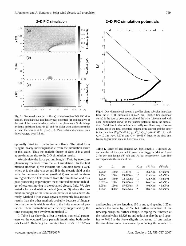
Figure3 shows the saturated state of the 2-D PIC simula-tion in our baseline run. The ion density (top panel) clearlyshows how incoming ions are repelled by the wire potentialand an ion deflection pattern develops, the shape of whichmuch resembles the familiar magnetosphere-solar wind in-teraction. The middle and bottom panels show the totaland plasma-only potentials, respectively. These are remark-ably symmetrical inx, i.e. the potential in the region whereprotons are most efficiently deflected is nearly cylindricallysymmetric. Thus the calculations of Sects. 2 and 3 remainwell valid also when the solar wind is introduced, although,it must be remarked, a small deviation from symmetry is thevery agent which produces the force acting on the wire.

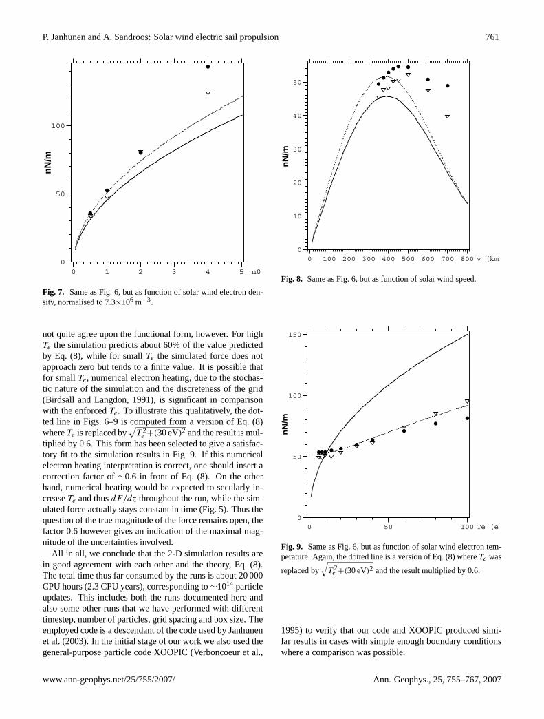
One-dimensional potential profiles along the subsolar line(x-axis) as taken from the 2-D simulation are shown in Fig.4.The vacuum potential of the wire (Eq.1, dashed) looks lin-ear in this plot where the x-axis is logarithmic. The plasmapotential (curve marked with heavy dots) varies smoothly.Both x>0 andx<0 branches are plotted in the figure, butthey virtually overlap in this scale, which is another manifes-tation of said high degree of cylindrical symmetry. The re-maining curve shows the total potential together with Eq. (2)



0

50

100

150

y (m

)

Ion

Den

s (c

m−3

)

0

50

100

150

200

250

0

50

100

150

y (m

)

To

talP

ot

(kV

)

0.01

0.1

1

−150 −100 −50 0 50 100 150 x (m)

0

50

100

150

y (m

)

−Pla

smaP

ot

(kV

)

0

0.5

1

1.5

2

2−D PIC simulation

(a)

(b)

(c)

Fig. 3. Saturated state (att=20 ms) of the baseline 2-D PIC sim-ulation. Instantaneous ion density(a), potential(b) and negative ofthe part of the potential which is due to the plasma(c). Scale is log-arithmic in (b) and linear in (a) and (c). Solar wind arrives from theleft and the wire is at(x, y)=(0, 0). Panels (b) and (c) have beentime averaged over 0.5 ms.

optimally fitted to it (including an offset). The fitted formis again nearly indistinguishable from the simulation curvein this scale. Thus the analytic theory of Sect. 2 is a goodapproximation also to the 2-D simulation results.

We calculate the force per unit lengthdF/dz by two com-plementary methods from the 2-D simulation. In the firstmethod (method 1) we evaluate the Coulomb forceF=qEwhereq is the wire charge andE is the electric field at thewire. In the second method (method 2) we record the time-averaged electric field pattern from the simulation and as apost-processing step compute the x-directed momentum bud-get of test ions moving in the obtained electric field. We alsotested a force calculation method (method 3) where the mo-mentum budget of the simulation particles is considered di-rectly. Method 3 (not shown) gives consistently less accurateresults than the other methods probably because of fluctua-tions in the fields which are due to the finite number of par-ticles. These fluctuations are efficiently suppressed by thetime-averaging step involved in method 2.

In Table 1 we show the effect of various numerical param-eters on the obtained force per unit length using both meth-ods 1 and 2. Reducing the timestep from 31.25 to 15.625 ns

1 10 100 r (m)

−2

−1

0

1

2

3

4

5

kV

2−D PIC simulation potentials

Fig. 4. One-dimensional potential profiles along subsolar line takenfrom the 2-D PIC simulation att=20 ms. Dashed line (topmostcurve) is the source potential profile of the wire. Line marked withdots (bottommost curve) is the plasma potential from the simula-tion. Solid line in the middle is actually two lines very close to-gether, one is the total potential (plasma plus source) and the otheris the function(V0/2)ln(1+(r0/r)2)/ln(r0/rw))+C (Eq. 2) withrw=10µm, r0=19.97 m andC=−10.68 V fitted to the first one.Notice logarithmic scale in horizontal axis.

Table 1. Effect of grid spacing1x, box lengthLx , timestep1t

and number of ions per cell in solar windNcell on Method 1 and2 for per unit lengthdF1/dz and F2/dz, respectively. Last linecorresponds to the standard run.

1x Lx 1t Ncell dF1/dz dF2/dz

1.25 m 160 m 31.25 ns 10 56 nN/m 57 nN/m1.25 m 160 m 15.625 ns 10 41 nN/m 45 nN/m1.25 m 160 m 7.8125 ns 10 42 nN/m 44 nN/m0.625 m 160 m 15.625 ns 10 44 nN/m 48 nN/m1.25 m 160 m 15.625 ns 5 40 nN/m 41 nN/m1.25 m 320 m 15.625 ns 20 48 nN/m 53 nN/m

and keeping the box length at 160 m and grid spacing 1.25 mreduces the force by∼25%, but further reduction of thetimestep brings no further change. Keeping the timestep atthe reduced value 15.625 ns and reducing also the grid spac-ing to 0.625 m the force slightly increases. If one makesthe simulation more inaccurate by reducing the number of



0 10 20 30 40 t (ms0

10

20

30

40

50

60

70

80

nN

/m

Force per length from 2−D PIC

Fig. 5. Force per unit length from 2-D PIC simulation as a functionof time using the Coulomb force method (method 1, dotted) andthe particle momentum method averaged over 20–40 ms (method 2,dashed). The risetime of the wire potential was set to 5 ms. Thesolid line shows the model result from Eq. (8).

particles per grid cell from 10 to 5, the force gets slightly re-duced. In the baseline run (last line of Table 1) we thus use20 ions per cell in the undisturbed solar wind to ensure thattheir number is sufficient and use a box length of 320 m tohave some additional safety margin in terms of the domainsize as well. This safety margin is good to have when wenext start varying the solar wind parametres and the electronsheath (potential structure) size starts to vary as well.

The force by methods 1 and 2 from the baseline run isshown in Fig.5 as a function of time. The expected resultfrom Eq. (8) is shown by solid line and the method 2 result,averaged over 20–40 ms, is shown by a dashed line. In thiscase, with all methods the simulation-based force is some-what larger than the theoretical formula. The data points inother figures show time averaged quantities where the aver-aging is carried out from 20 to 40 ms, thus the initial tran-sients at∼6 ms do not contribute to the results.

The potential in Figs.5, 7, 8 and9 is about 14.5 kV. Thetotal potential in the simulation box is a sum of the bare wirepotential which is imposed and known and the plasma poten-tial which is calculated during the simulation. The potentialdifferenceV0 between the wire surface and the solar windplasma must therefore be calculated from the simulation af-terwards. TheV0 values thus obtained differ slightly fromcase to case. Although not numerically significant, we com-pensate for the differences by scaling with Eq. (8) in Figs.7,8 and9.

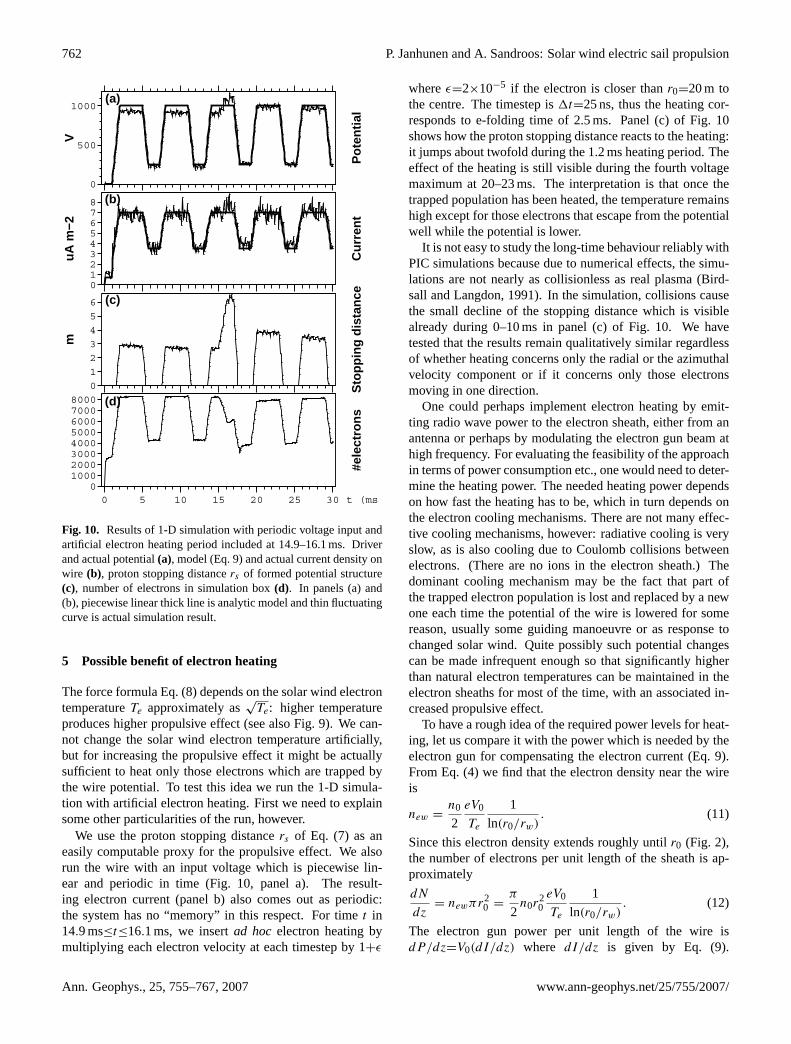
Figure6 shows the simulated force as a function of the po-tentialV0. Again, method 1 (triangles) and method 2 (dots)are compared with the theoretical curve, Eq. (8). In addition

0 5 10 15 20 V0 (kV0

10

20

30

40

50

60

70

80

nN

/mFig. 6. Force per unit length from 2-D PIC simulation as a functionof wire voltageV0 compared with model prediction. Force calcu-lated from electric field at wire (method 1, triangles), from parti-cle momentum balance (method 2, dots), force from and Eq. (8)(solid) and force from Eq (8) multiplied by 0.6 andTe replaced by√

T 2e +(30 eV)2 (dotted). Motivation for dotted line expression is

given in connection with Fig.9. In each case the risetime was 5 ms,the run was continued until 40 ms and the forces were averaged at20–40 ms.

we show a version of Eq. (8) which is multiplied by 0.6 andwhereTe is replaced by

√T 2

e +(30 eV)2 by dotted line; themotivation for this is given in connection with Fig.9 below.One sees that the agreement between the theoretical curvesand the simulation (both methods 1 and 2) is satisfactorilygood.

Figure7 is similar to Fig.6 except that now we vary thesolar wind electron densityn0 instead of the voltage. Theagreement between theory, Eq. (8), and simulation is goodfor low and normal density and becomes worse for higherdensities. This is probably due to the fact that for high elec-tron density, the size of the electron sheath (potential struc-ture) is smaller so that one should use a finer grid to resolveit properly.

In Fig. 8 we vary the solar wind speed. Now the optimalforce position occurs at somewhat different solar wind speedin the theory and the simulation. Again, the discrepancy be-tween methods 1 and 2 is largest at the highest solar windspeed, which is probably again due to the fact that the sizeof the electron sheath is smaller and more difficult for thesimulation to resolve.

Finally, in Fig.9 we vary the solar wind electron temper-atureTe. All methods predict that the force increases whenthe electrons become hotter. The simulation and theory do



0 1 2 3 4 5 n00

50

100

nN

/m

Fig. 7. Same as Fig.6, but as function of solar wind electron den-sity, normalised to 7.3×106 m−3.

not quite agree upon the functional form, however. For highTe the simulation predicts about 60% of the value predictedby Eq. (8), while for smallTe the simulated force does notapproach zero but tends to a finite value. It is possible thatfor smallTe, numerical electron heating, due to the stochas-tic nature of the simulation and the discreteness of the grid(Birdsall and Langdon, 1991), is significant in comparisonwith the enforcedTe. To illustrate this qualitatively, the dot-ted line in Figs.6–9 is computed from a version of Eq. (8)whereTe is replaced by

√T 2

e +(30 eV)2 and the result is mul-tiplied by 0.6. This form has been selected to give a satisfac-tory fit to the simulation results in Fig.9. If this numericalelectron heating interpretation is correct, one should insert acorrection factor of∼0.6 in front of Eq. (8). On the otherhand, numerical heating would be expected to secularly in-creaseTe and thusdF/dz throughout the run, while the sim-ulated force actually stays constant in time (Fig.5). Thus thequestion of the true magnitude of the force remains open, thefactor 0.6 however gives an indication of the maximal mag-nitude of the uncertainties involved.

All in all, we conclude that the 2-D simulation results arein good agreement with each other and the theory, Eq. (8).The total time thus far consumed by the runs is about 20 000CPU hours (2.3 CPU years), corresponding to∼1014 particleupdates. This includes both the runs documented here andalso some other runs that we have performed with differenttimestep, number of particles, grid spacing and box size. Theemployed code is a descendant of the code used byJanhunenet al.(2003). In the initial stage of our work we also used thegeneral-purpose particle code XOOPIC (Verboncoeur et al.,

0 100 200 300 400 500 600 700 800 v (km0

10

20

30

40

50

nN

/mFig. 8. Same as Fig.6, but as function of solar wind speed.

0 50 100 Te (eV0

50

100

150

nN

/m

Fig. 9. Same as Fig.6, but as function of solar wind electron tem-perature. Again, the dotted line is a version of Eq. (8) whereTe was

replaced by√

T 2e +(30 eV)2 and the result multiplied by 0.6.

1995) to verify that our code and XOOPIC produced simi-lar results in cases with simple enough boundary conditionswhere a comparison was possible.



0

500

1000

V

Po

ten

tial

012345678

uA

m−2

Cu

rren

t

0123456

m

Sto

pp

ing

dis

tan

ce

0 5 10 15 20 25 30 t (ms0

10002000300040005000600070008000

#ele

ctro

ns

(a)

(b)

(c)

(d)

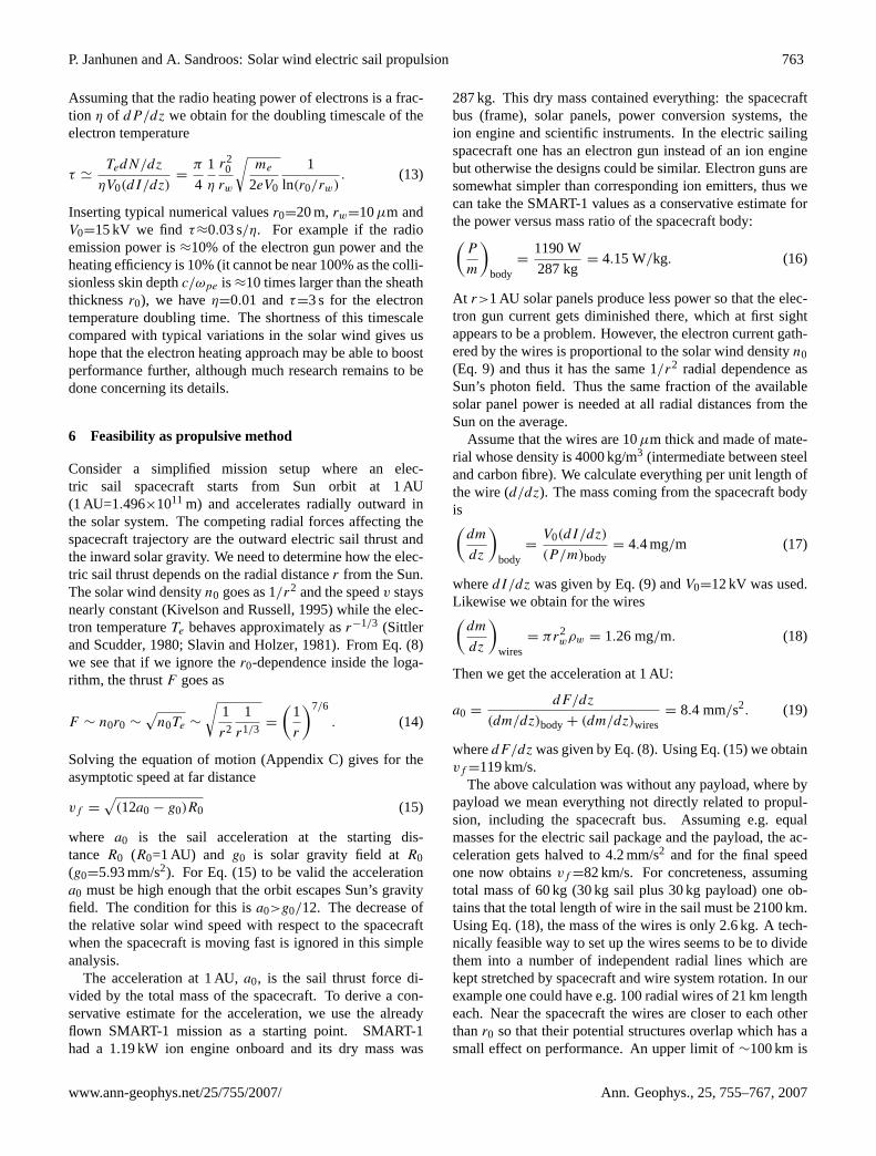
Fig. 10. Results of 1-D simulation with periodic voltage input andartificial electron heating period included at 14.9–16.1 ms. Driverand actual potential(a), model (Eq.9) and actual current density onwire (b), proton stopping distancers of formed potential structure(c), number of electrons in simulation box(d). In panels (a) and(b), piecewise linear thick line is analytic model and thin fluctuatingcurve is actual simulation result.

5 Possible benefit of electron heating

The force formula Eq. (8) depends on the solar wind electrontemperatureTe approximately as

√Te: higher temperature

produces higher propulsive effect (see also Fig.9). We can-not change the solar wind electron temperature artificially,but for increasing the propulsive effect it might be actuallysufficient to heat only those electrons which are trapped bythe wire potential. To test this idea we run the 1-D simula-tion with artificial electron heating. First we need to explainsome other particularities of the run, however.

We use the proton stopping distancers of Eq. (7) as aneasily computable proxy for the propulsive effect. We alsorun the wire with an input voltage which is piecewise lin-ear and periodic in time (Fig.10, panel a). The result-ing electron current (panel b) also comes out as periodic:the system has no “memory” in this respect. For timet in14.9 ms≤t≤16.1 ms, we insertad hocelectron heating bymultiplying each electron velocity at each timestep by 1+ε

whereε=2×10−5 if the electron is closer thanr0=20 m tothe centre. The timestep is1t=25 ns, thus the heating cor-responds to e-folding time of 2.5 ms. Panel (c) of Fig.10shows how the proton stopping distance reacts to the heating:it jumps about twofold during the 1.2 ms heating period. Theeffect of the heating is still visible during the fourth voltagemaximum at 20–23 ms. The interpretation is that once thetrapped population has been heated, the temperature remainshigh except for those electrons that escape from the potentialwell while the potential is lower.

It is not easy to study the long-time behaviour reliably withPIC simulations because due to numerical effects, the simu-lations are not nearly as collisionless as real plasma (Bird-sall and Langdon, 1991). In the simulation, collisions causethe small decline of the stopping distance which is visiblealready during 0–10 ms in panel (c) of Fig.10. We havetested that the results remain qualitatively similar regardlessof whether heating concerns only the radial or the azimuthalvelocity component or if it concerns only those electronsmoving in one direction.

One could perhaps implement electron heating by emit-ting radio wave power to the electron sheath, either from anantenna or perhaps by modulating the electron gun beam athigh frequency. For evaluating the feasibility of the approachin terms of power consumption etc., one would need to deter-mine the heating power. The needed heating power dependson how fast the heating has to be, which in turn depends onthe electron cooling mechanisms. There are not many effec-tive cooling mechanisms, however: radiative cooling is veryslow, as is also cooling due to Coulomb collisions betweenelectrons. (There are no ions in the electron sheath.) Thedominant cooling mechanism may be the fact that part ofthe trapped electron population is lost and replaced by a newone each time the potential of the wire is lowered for somereason, usually some guiding manoeuvre or as response tochanged solar wind. Quite possibly such potential changescan be made infrequent enough so that significantly higherthan natural electron temperatures can be maintained in theelectron sheaths for most of the time, with an associated in-creased propulsive effect.

To have a rough idea of the required power levels for heat-ing, let us compare it with the power which is needed by theelectron gun for compensating the electron current (Eq.9).From Eq. (4) we find that the electron density near the wireis

new =n0

2

eV0

Te

1

ln(r0/rw). (11)

Since this electron density extends roughly untilr0 (Fig. 2),the number of electrons per unit length of the sheath is ap-proximately

dN

dz= newπr2

0 =π

2n0r

20eV0

Te

1

ln(r0/rw). (12)

The electron gun power per unit length of the wire isdP/dz=V0(dI/dz) where dI/dz is given by Eq. (9).



Assuming that the radio heating power of electrons is a frac-tion η of dP/dz we obtain for the doubling timescale of theelectron temperature

τ 'TedN/dz

ηV0(dI/dz)=

π

4

1

η

r20

rw

√me

2eV0

1

ln(r0/rw). (13)

Inserting typical numerical valuesr0=20 m,rw=10µm andV0=15 kV we find τ≈0.03 s/η. For example if the radioemission power is≈10% of the electron gun power and theheating efficiency is 10% (it cannot be near 100% as the colli-sionless skin depthc/ωpe is ≈10 times larger than the sheaththicknessr0), we haveη=0.01 andτ=3 s for the electrontemperature doubling time. The shortness of this timescalecompared with typical variations in the solar wind gives ushope that the electron heating approach may be able to boostperformance further, although much research remains to bedone concerning its details.

6 Feasibility as propulsive method

Consider a simplified mission setup where an elec-tric sail spacecraft starts from Sun orbit at 1 AU(1 AU=1.496×1011 m) and accelerates radially outward inthe solar system. The competing radial forces affecting thespacecraft trajectory are the outward electric sail thrust andthe inward solar gravity. We need to determine how the elec-tric sail thrust depends on the radial distancer from the Sun.The solar wind densityn0 goes as 1/r2 and the speedv staysnearly constant (Kivelson and Russell, 1995) while the elec-tron temperatureTe behaves approximately asr−1/3 (Sittlerand Scudder, 1980; Slavin and Holzer, 1981). From Eq. (8)we see that if we ignore ther0-dependence inside the loga-rithm, the thrustF goes as

F ∼ n0r0 ∼

√n0Te ∼

√1

r2

1

r1/3=

(1

r

)7/6

. (14)

Solving the equation of motion (Appendix C) gives for theasymptotic speed at far distance

vf =√

(12a0 − g0)R0 (15)

where a0 is the sail acceleration at the starting dis-tance R0 (R0=1 AU) and g0 is solar gravity field atR0(g0=5.93 mm/s2). For Eq. (15) to be valid the accelerationa0 must be high enough that the orbit escapes Sun’s gravityfield. The condition for this isa0>g0/12. The decrease ofthe relative solar wind speed with respect to the spacecraftwhen the spacecraft is moving fast is ignored in this simpleanalysis.

The acceleration at 1 AU,a0, is the sail thrust force di-vided by the total mass of the spacecraft. To derive a con-servative estimate for the acceleration, we use the alreadyflown SMART-1 mission as a starting point. SMART-1had a 1.19 kW ion engine onboard and its dry mass was

287 kg. This dry mass contained everything: the spacecraftbus (frame), solar panels, power conversion systems, theion engine and scientific instruments. In the electric sailingspacecraft one has an electron gun instead of an ion enginebut otherwise the designs could be similar. Electron guns aresomewhat simpler than corresponding ion emitters, thus wecan take the SMART-1 values as a conservative estimate forthe power versus mass ratio of the spacecraft body:(

P

m

)body

=1190 W

287 kg= 4.15 W/kg. (16)

At r>1 AU solar panels produce less power so that the elec-tron gun current gets diminished there, which at first sightappears to be a problem. However, the electron current gath-ered by the wires is proportional to the solar wind densityn0(Eq. 9) and thus it has the same 1/r2 radial dependence asSun’s photon field. Thus the same fraction of the availablesolar panel power is needed at all radial distances from theSun on the average.

Assume that the wires are 10µm thick and made of mate-rial whose density is 4000 kg/m3 (intermediate between steeland carbon fibre). We calculate everything per unit length ofthe wire (d/dz). The mass coming from the spacecraft bodyis(

dm

dz

)body

=V0(dI/dz)

(P/m)body= 4.4 mg/m (17)

wheredI/dz was given by Eq. (9) andV0=12 kV was used.Likewise we obtain for the wires(

dm

dz

)wires

= πr2wρw = 1.26 mg/m. (18)

Then we get the acceleration at 1 AU:

a0 =dF/dz

(dm/dz)body + (dm/dz)wires= 8.4 mm/s2. (19)

wheredF/dz was given by Eq. (8). Using Eq. (15) we obtainvf =119 km/s.

The above calculation was without any payload, where bypayload we mean everything not directly related to propul-sion, including the spacecraft bus. Assuming e.g. equalmasses for the electric sail package and the payload, the ac-celeration gets halved to 4.2 mm/s2 and for the final speedone now obtainsvf =82 km/s. For concreteness, assumingtotal mass of 60 kg (30 kg sail plus 30 kg payload) one ob-tains that the total length of wire in the sail must be 2100 km.Using Eq. (18), the mass of the wires is only 2.6 kg. A tech-nically feasible way to set up the wires seems to be to dividethem into a number of independent radial lines which arekept stretched by spacecraft and wire system rotation. In ourexample one could have e.g. 100 radial wires of 21 km lengtheach. Near the spacecraft the wires are closer to each otherthanr0 so that their potential structures overlap which has asmall effect on performance. An upper limit of∼100 km is



set by the material conductivity of the wires (they must beable to carry the arriving electron current) while the numberof wires is in practise limited by technical aspects.

With 82 km/s speed (17.2 AU/year) one would reach Plutoorbit in two years.

We have made more elaborate calculations of the perfor-mance where we among other things use real solar wind dataand take into account the wire multiplicity which is neededfor micrometeor resistance (Hoyt and Forward, 2001). Theseconsiderations typically reduce the final speeds to some ex-tent, but broadly speaking, using different assumptions theresulting final speeds generally fall in the range 40–100 km/sfor payloads up to∼50 kg, assuming power versus mass ra-tios that correspond to today’s flight-proved components forthe spacecraft body.

Here we did not include a correction factor of 0.6 inEq. (8), whose presence would explain better the electrontemperature behaviour (see the second-last paragraph ofSect. 4 and Fig.9). The final speed has approximately asquare root dependence on the acceleration, so with this cor-rection the final speed in the above example would become60 km/s instead of 82 km/s. On the other hand, we also didnot assume any electron heating. If electron heating would beimplemented successfully, the performance could be larger,possibly by a significant amount.

The results of this paper should be accurate enough forevaluating the overall feasibility of the electric sail. For de-tailed mission planning, space experiments with a prototypesail would be needed.

6.1 Comparison with solar sail

A comparison of the electric sail performance with other pro-posed propulsion methods such as electric propulsion is out-side the scope of this paper. However, the solar radiationpressure sail is in many respects similar enough to allow fora rather simple quantitative comparison.

An ideal (i.e. fully reflecting) solar sail receives a radi-ation pressure force of 9µN/m2 at 1 AU distance from theSun. Let us calculate how thin a solar sail should be, to reachthe same specific acceleration as an electric sail wire pluselectron gun subsystems (Eq.19). Using the above exam-ple with 82 km/s final speed, one obtains that the solar sailshould have an areal density of 1.1 g/m2, which translates to200 nm thickness if the material is aluminium and 50% ofthe mass is assumed to go to support structures. This is 5–10times thinner than present technology.

Although similar in many respects, the solar sail and theelectric sail also have some important operational differ-ences. When moving away from the Sun, the electric sailforce decays as 1/r7/6 which is slower than the solar sail1/r2 dependence. On the other hand the solar sail can beused also inside planetary magnetospheres, whereas the elec-tric sail needs the solar wind to operate.

6.2 Possible missions

Assuming that no technological obstacles will arise thatmarkedly alter the performance of the electric sail from theabove estimates, which type of missions could benefit fromit? The electric sail much resembles the solar sail in thatit provides small but inexhaustible thrust which is directedoutward from the Sun, with a modest control of the thrustdirection allowed (probably by a few tens of degrees). Firstand foremost the electric sail can thus be used for missionsgoing outward in the solar system and aiming for>50 km/sfinal speed, such as missions going out of the heliosphere andfast and cheap flyby missions of any target in the outer solarsystem. Secondly, by inclining the sail to some angle it canalso be used to spiral inward in the solar system to study e.g.Mercury and Sun. Also a nonzero inclination with respect tothe ecliptic plane is possible to achieve which may be ben-eficial for observing the Sun. Also the return trip back toEarth from the inner solar system is possible, as is cruisingback and forth in the inner solar system and visiting multipletargets such as asteroids. Thirdly, the electric sail could beused to implement a solar wind monitoring spacecraft whichis placed permanently between Earth and Sun at somewhereelse than the Lagrange point, thus providing a space weatherservice with more than one hour of warning time. Propul-sion and data taking phases probably must be interleaved be-cause ion measurements are not possible when the platformis charged to high positive voltage, although the plasma den-sity and dynamic pressure of the solar wind can probably besensed by an electron detector and accelerometer even whenthe electric sail voltage is turned on.

Once accelerated to a high outward speed an electric sail-ing spacecraft cannot by itself stop to orbit a remote targetbecause the radial component of the thrust is always posi-tive. For stopping under those circumstances one has to useaerocapture or some other traditional technique. Althoughthe electric sail does not provide a marked speed benefit forsuch missions, being propellantless it might still provide costsaving; this remains to be studied.

In interstellar space the plasma flow is rather slow. Thusthe electric sail cannot be used for acceleration, but it can in-stead be used for braking the spacecraft. There are some con-cepts such as the laser or microwave sail which are designedto “shoot” a small probe at ultrahigh speed towards e.g. aremote solar system. In these concepts the power source isat Earth so that the accelerated probe needs no propulsiveenergy source. Stopping the probe at the remote target isvery difficult, however, if one has to rely on power beamedfrom the starting point. The electric sail might then providea feasible stopping mechanism for such mission concepts. Inother words, one would shoot a probe to another solar sys-tem at ultrahigh speed using a massive and powerful laseror microwave source installed in near-Earth space, brake theprobe before the target by the electric sail action in the in-terstellar plasma and finally explore the extrasolar planetary



system with the help of the electric sail and the stellar wind.A similar idea was proposed byZubrin and Andrews(1990)for their magnetic version of the solar wind sail.

7 Conclusions

We have verified using different particle simulations that thetheory presented in Sect. 2, in particular Eq. (8), is very likelyto be a good approximation to the true force exerted by thesolar wind to a thin charged wire. The main independent ver-ifications were the following: (A) The potential expression(2) is in very good agreement with 1-D simulations wherethere is no solar wind flow. (B) The 2-D simulations are inrather good agreement with the force formula (8).

The electron current gathered by the wire or wire systemis likely to be well approximated by the OML theory result,Eq. (9), for reasons explained at the end of Sect. 2.1.

Although the technical and engineering details of how todesign a working electric sail are outside the scope of thispaper, it is our belief that these issues can be resolved withouta need to extrapolate on the current level of technology.

Considering the performance estimates of Sect. 6, wethink that it is no exaggeration to say that the electric sailis an extremely promising new propulsion technique whoseapplication area includes (but is not limited to) scientific mis-sions with small to medium payloads where unprecedentedlyhigh final speeds 40–100 km/s are required to accomplish theobjectives. As a further bonus, if electron heating turns out tobe successful it may increase the performance even further.

Appendix A

Effective electric radius

Here we consider how to calculate the effective electric ra-dius of a multicomponent wire. ConsiderN wires whose allmutual distances are equal toh. The wires are in vacuum andkept in potentialV0 with the requirement that the total poten-tial vanishes atr=r0 wherer0�h�rw andrw is the singlewire radius. The caseN=2 corresponds to a double wire andN=3 corresponds to a triple wire. In the latter case the wiresform an equilateral triangle in the perpendicular plane. Thevacuum assumption can be made becauseh�r0.

In vacuum the potential of a single wire is

V (r) = V0ln(r0/r)

ln(r0/rw). (A1)

The corresponding electric field is

E(r) = −V ′(r) =V0/r

ln(r0/rw). (A2)

At the wire surface the electric field is

E0 = E(rw) =V0/rw

ln(r0/rw). (A3)

Application of Gauß’ law gives the line chargeλ as

λ =

(2πε0

ln(r0/rw)

)V0. (A4)

This equation serves as the definition of the effective wirewidth: if a multiple wire system has total line chargeλ whilebeing in potentialV0, its effective widthr∗

w is by definition

r∗w = r0 exp

(−2πε0V0

λ

). (A5)

If the total line charge of the wire system isλ, due to sym-metry each subwire has line chargeλ/N . The potential at thesurface of a subwire is then

V0 =λ

2πε0

[1

Nln

(r0

rw

)+

(N − 1)

Nln( r0

h

)]. (A6)

Here we used Eq. (A4). The first term in Eq. (A6) is due tothe subwire itself and the second term is the potential causedby the other subwires which are at distanceh. SubstitutingEq. (A6) in Eq. (A5) we obtain after simplification

r∗w = r1/N

w h1−1/N . (A7)

For double wire (N=2) we thus haver∗w=

√rwh (geometric

average) and for triple wire (N=3) we obtainr∗w=

(rwh2

)1/3.

For example ifrw=10µm andh=1 cm, the double wire ef-fective radius isr∗

w=0.3 mm.

Appendix B

Electric current gathered by single wire

In this appendix we derive Eq. (9). Consider a wire of ra-dius rw which resides in potentialV0 and an incident coldelectron beam with densityn and speedv0. Assume the po-tential pattern around the wire is cylindrically symmetric sothat the attractive Coulomb force is a central force and soboth the total energy and angular momentum of incomingelectrons are conserved. Assume also thatv0�vmax wherevmax=

√2eV0/me is the speed of those electrons that nearly

touch the wire. Let the incoming electron arrive with im-pact parametery=b with x-directed velocity (Fig.B1). Thenthe limiting case when the electron just barely collides withthe wire is reached when its velocity at the time of closestapproach is equal tovmax in magnitude. At that time theelectron’s orbit is tangential to the wire and thus its angularmomentumL is L=mevmaxrw, which must be equal to theoriginal angular momentummev0b due to conservation ofL.Thus we obtain

blimit = rw

(vmax

v0

). (B1)



−3 −2 −1 0 1−3

−2

−1

0

1

2

3

x

y

3

2

1

0

1

2

3

Fig. B1. Geometry of Appendix B. Electrons arrive from the left.Those with small enough impact parameter (initial y-coordinate)hit the wire (solid lines) while others pass by it (dashed lines). Thescales are arbitrary.

An electron collides with the wire if and only if the absolutevalue of its impact parameter is less thanblimit . Thus theelectron current gathered by the wire per unit length is

dI

dz= (env0) (2blimit ) = envmax2rw = en

√eV0

me

2rw (B2)

which is Eq. (9). The result depends only on the beam den-sity n but not on its speedv0 or incoming direction. There-fore it holds for any electron velocity distribution as long asall the speeds are much lower thanvmax because such a dis-tribution can be thought to be composed of a large number ofsmall-density beams with different incoming velocities.

Appendix C

Solving spacecraft trajectory

Consider a spacecraft starting from circular solar orbit atR0=1 AU. Its equation of motion is

r = a−g+L2

r3= a0

(R0

r

)α

−g0

(R0

r

)2

+g0

(R0

r

)3

(C1)

wherea0 is the sail acceleration atR0, g0=0.00593 m/s2 isSun’s gravity field atR0 and the exponentα=7/6 (Eq.14).Multiplying by r we obtain

r r =d

dt

(1

2r2)

= a0Rα0 r−α r − g0R

20

r

r2+ g0R

30

r

r3. (C2)

Integrating with respect to timet from 0 tot we arrive at

1

2r2

= a0Rα0

(r1−α

1 − α−

R1−α0

1 − α

)

− g0R20

(1

R0−

1

r

)+

1

2g0R

30

(1

R20

−1

r2

)(C3)

Forr�R0 the negative powers ofr vanish so we are left with

1

2r2

=a0R0

α − 1−

1

2g0R0 (C4)

which can be rearranged to give

r = vf =

√(2a0

α − 1− g0

)R0 =

√(12a0 − g0)R0 (C5)

which is Eq. (15).

Acknowledgements.The authors would like to thank R. Vainiofor useful discussions and for comments that have improved themanuscript. R. Hoyt, M. Zavyalov and V. Linkin provided use-ful technical information. Discussions with E. Keski-Vakkuri,H. Koskinen, H. Laakso, K. Nordlund, J. Polkko, W. Schmidt,J. Silen, M. Uspensky and A. Viljanen are also gratefully acknowl-edged. The work of A. Sandroos was partly supported by grantsfrom the Academy of Finland and the electric sail work by the Foun-dation for Finnish Inventions and the Vaisala Foundation.

Topical Editor I. A. Daglis thanks two referees for their help inevaluating this paper.

References

Allen, J. E.: Probe theory – the orbital motion approach, PhysicaScripta, 45, 497–503, 1992.

Birdsall, C. K. and Langdon, A. B.: Plasma physics via computersimulation, Adam Hilger, New York, 1991.

Hoyt, R. and Forward, R. L.: Alternate interconnection Hoytetherfailure resistant multiline tether, US Pat. 6286788 B1, 2001.

Kivelson, M. G. and Russell, C. T. (Eds.): Introduction to spacephysics, Cambridge, 1995.



Janhunen, P., Olsson, A., Vaivads, A., and Peterson, W. K.: Gener-ation of Bernstein waves by ion shell distributions in the auroralregion, Ann. Geophys., 21, 881–891, 2003,http://www.ann-geophys.net/21/881/2003/.

Janhunen, P.: Electric sail for spacecraft propulsion, Journal ofPropulsion and Power, 20(4), 763–764, 2004.

Mott-Smith, H. M. and Langmuir, I.: The theory of collectors ingaseous discharges, Phys. Rev., 28, 727–763, 1926.

Sittler, E. C. and Scudder, J. D.: An empirical polytrope law forsolar wind thermal electrons between 0.45 and 4.76 AU: Voyager2 and Mariner 10, J. Geophys. Res., 85, 5131–5137, 1980.

Slavin, J. A. and Holzer, R. E.: Solar wind flow about the terrestrialplanets, I. Modeling bow shock position and shape, J. Geophys.Res., 86, 11 401–11 418, 1981.

Verboncoeur, J. P., Langdon, A. B., and Gladd, N. T.: An object-oriented electromagnetic PIC code, Comput. Phys. Commun.,87, 199–211, 1995.

Zubrin, R. M. and Andrews, D. G.: Magnetic sails and interstellartravel, British Interplanetary Society Journal, 43, 265–272, 1990.

Zubrin, R. M. and Andrews, D. G.: Magnetic sails and interplan-etary travel, Journal of Spacecraft and Rockets, 28, 197–203,1991.


http://www.ann-geophys.net/21/881/2003/

simulation study of solar wind push on a charged wire...

Documents