simulationmodelingmethodology:principlesand ... · pdf...
TRANSCRIPT

SIMULATION MODELING METHODOLOGY: PRINCIPLES AND
ETIOLOGY OF DECISION SUPPORT
by
Ernest H. Page, Jr.
Dissertation submitted to the faculty of the
Virginia Polytechnic Institute and State University
in partial fulfillment of the requirements for the degree of
Doctor of Philosophy
in
Computer Science
Approved:
Richard E. Nance, Chairman
Marc Abrams
Osman Balci
James D. Arthur
C. Michael Overstreet
September 1994
Blacksburg, Virginia

SIMULATION MODELING METHODOLOGY: PRINCIPLES AND
ETIOLOGY OF DECISION SUPPORT
by
Ernest H. Page, Jr.
Committee Chairman: Richard E. Nance
Department of Computer Science
(ABSTRACT)
Investigation in discrete event simulation modeling methodology has persisted for over
thirty years. Fundamental is the recognition that the overriding objectives for simulation
must involve decision support. Rapidly advancing technology is today exerting major in-
fluences on the course of simulation in many areas, e.g. distributed interactive simulation
and parallel discrete event simulation, and evidence suggests that the role of decision sup-
port is being subjugated to accommodate new technologies and system-level constraints.
Two questions are addressed by this research: (1) can the existing theories of modeling
methodology contribute to these new types of simulation, and (2) how, if at all, should di-
rections of modeling methodological research be redefined to support the needs of advancing
technology.
Requirements for a next-generation modeling framework (NGMF) are proposed, and
a model development abstraction is defined to support the framework. The abstraction
identifies three levels of model representation: (1) modeler-generated specifications, (2)
transformed specifications, and (3) implementations. This hierarchy may be envisaged as
consisting of either a set of narrow-spectrum languages, or a single wide-spectrum language.
Existing formal approaches to discrete event simulation modeling are surveyed and evaluated
with respect to the NGMF requirements. All are found deficient in one or more areas.
The Conical Methodology (CM), in conjunction with the Condition Specification (CS), is
identified as a possible NGMF candidate. Initial assessment of the CS relative to the model
development abstraction indicates that the CS is most suited for the middle level of the
hierarchy of representations – specifically functioning as a form for analysis.
The CS is extended to provide wide-spectrum support throughout the entire hierarchy
via revisions of its supportive facilities for both model representation and model execu-
tion. Evaluation of the pertinent model representation concepts is accomplished through a
complete development of four models. The collection of primitives for the CS is extended
to support CM facilities for set definition. A higher-level form for the report specification
is defined, and the concept of an augmented specification is outlined whereby the object

specification and transition specification may be automatically transformed to include the
objects, attributes and actions necessary to provide statistics gathering. An experiment
specification is also proposed to capture details, e.g. the condition for the start of steady
state, necessary to produce an experimental model.
In order to provide support for model implementation, the semantic rules for the CS are
refined. Based on a model of computation provided by the action cluster incidence graph
(ACIG), an implementation structure referred to as a direct execution of action clusters
(DEAC) simulation is defined. A DEAC simulation is simply an execution of an augmented
CS transition specification. Two algorithms for DEAC simulations are presented.
Support for parallelizing model execution is also investigated. Parallel discrete event
simulation (PDES) is presented as a case study. PDES research is evaluated from the
modeling methodological perspective espoused by this effort, and differences are noted in
two areas: (1) the enunciation of the relationship between simulation and decision support,
and the guidance provided by the life cycle in this context, and (2) the focus of the devel-
opment effort. Recommendations are made for PDES research to be reconciled with the
“mainstream” of DES.
The capability of incorporating parallel execution within the CM/CS approach is inves-
tigated. A new characterization of inherent parallelism is given, based on the time and state
relationships identified in prior research. Two types of inherent parallelism are described:
(1) inherent event parallelism, which relates to the independence of attribute value changes
that occur during a given instant, and (2) inherent activity parallelism, which relates to
the independence of attribute value changes that occur over all instants of a given model
execution. An analogy between an ACIG and a Petri net is described, and a synchronous
model of parallel execution is developed based on this analogy. Revised definitions for the
concepts time ambiguity and state ambiguity in a CS are developed, and a necessary condi-
tion for state ambiguity is formulated. A critical path algorithm for parallel direct execution
of action clusters (PDEAC) simulations is constructed. The algorithm is an augmentation
of the standard DEAC algorithm and computes the synchronous critical path for a given
model representation. Finally, a PDEAC algorithm is described.

For Ernest H. Page, 1921 - 1977. We’re having a lovely time, wish you were here.
iv

Acknowledgements
To say that thanks is due my major advisor, Dick Nance, would be an egregious understate-
ment. During the past six years he has played the simultaneous roles of mentor, role model,
employer, friend, partner-in-crime, and father to me, and perhaps most importantly, he
has been “Nook” to my children. Similar sentiments apply to Marc Abrams, Sean Arthur,
Osman Balci and Mike Overstreet. All of these gentlemen have enriched my life beyond my
capacity to thank them. Clearly, of the many things I take with me from my tenure at this
university, the relationships I have built – both personal and professional, particularly with
the members of my committee – are most prized.
Thanks also should be expressed to my friends and comrades. I couldn’t possibly name them
all, but I must acknowledge Bobby Beamer and Lev Malakhoff, who I met on my first day
here in the fall of 1983 and who have been my friends ever since; Ken and Jennifer Landry,
good neighbors and gumbo cooks; Ben Keller, with whom I have often commiserated over a
calzone at Mike’s; and, of course, my golfing compatriots: Randy Love, Jamie Evans, Sean,
Dick, and my brother Tony Page.
As for family, I am indebted to my brother and his wife, Kim, for their friendship and
babysitting service. Tony should also be acknowledged for working out some of the math-
ematics in Chapter 6; Larry and Brenda Salyers, who are among my children’s favorite
grandparents, and who reminded me when I married their daughter that ‘this is not a loan’;
my uncle, Bill Baker, to whom I owe much, he has been both friend and father to me over
the years and he taught me the game of golf at the rate of $1-a-hole – not that I’m a slow
learner, but I believe my current debt structure is in the neighborhood of $100K; and my
mother, Barbara Page, who, other than during her reign as Virginia Tech Parent of the
Year, hasn’t been that insufferable.
Finally, I must thank my wife, Larenda, and children Julia and Ernie, who have too often
been neglected during the completion of this work.
v

Contents
1 INTRODUCTION 1
1.1 Problem Definition . . . . . . . . . . . . . . . . . . . . . . . . . . . . . . . 2
1.2 Thesis Objectives . . . . . . . . . . . . . . . . . . . . . . . . . . . . . . . . 4
1.3 Thesis Approach . . . . . . . . . . . . . . . . . . . . . . . . . . . . . . . . 4
1.4 Thesis Organization . . . . . . . . . . . . . . . . . . . . . . . . . . . . . . 6
1.5 Summary of Results . . . . . . . . . . . . . . . . . . . . . . . . . . . . . . 7
1.5.1 Modeling methodology . . . . . . . . . . . . . . . . . . . . . . . 8
1.5.2 Parallel discrete event simulation . . . . . . . . . . . . . . . . . . 9
2 DISCRETE EVENT SIMULATION TERMINOLOGY 10
3 A PHILOSOPHY OF MODEL DEVELOPMENT 14
3.1 A Modeling Methodological View of Discrete Event Simulation . . . . . . 15
3.1.1 What is simulation? . . . . . . . . . . . . . . . . . . . . . . . . . 15
3.1.2 Enhancing decision support through model quality management 16
3.1.2.1 Life cycle, paradigm and methodology . . . . . . . . . 17
3.1.2.2 A life-cycle model for simulation . . . . . . . . . . . . . 19
3.1.3 Some issues in model representation . . . . . . . . . . . . . . . . 21
3.1.3.1 The programming language impedance . . . . . . . . . 21
3.1.3.2 The conceptual framework problem . . . . . . . . . . . 22
3.2 An Environment for Simulation Model Development . . . . . . . . . . . . 23
3.3 A Next-Generation Framework for Model Development . . . . . . . . . . 24
3.3.1 Theories of model representation . . . . . . . . . . . . . . . . . . 25
3.3.1.1 Wide-spectrum versus narrow-spectrum languages . . . 25
3.3.1.2 Formal approaches . . . . . . . . . . . . . . . . . . . . 26
3.3.1.3 Graphical approaches . . . . . . . . . . . . . . . . . . . 26
3.3.2 Requirements for a next-generation modeling framework . . . . 27
vi

Contents
3.3.3 An abstraction based on a hierarchy of representations . . . . . 28
3.4 Summary . . . . . . . . . . . . . . . . . . . . . . . . . . . . . . . . . . . . 30
4 FORMAL APPROACHES TO DISCRETE EVENT SIMULATION 32
4.1 Preface . . . . . . . . . . . . . . . . . . . . . . . . . . . . . . . . . . . . . 32
4.1.1 A model classification scheme . . . . . . . . . . . . . . . . . . . 33
4.1.2 Formalism and discrete event models . . . . . . . . . . . . . . . 35
4.2 Lackner’s Formalism . . . . . . . . . . . . . . . . . . . . . . . . . . . . . . 35
4.2.1 Defining the theory . . . . . . . . . . . . . . . . . . . . . . . . . 36
4.2.1.1 The problem . . . . . . . . . . . . . . . . . . . . . . . . 36
4.2.1.2 System and state . . . . . . . . . . . . . . . . . . . . . 36
4.2.1.3 Weltansicht . . . . . . . . . . . . . . . . . . . . . . . . 37
4.2.2 The Change Calculus . . . . . . . . . . . . . . . . . . . . . . . . 37
4.2.3 Examples . . . . . . . . . . . . . . . . . . . . . . . . . . . . . . . 40
4.2.4 Evaluation . . . . . . . . . . . . . . . . . . . . . . . . . . . . . . 41
4.3 Systems Theoretic Approaches . . . . . . . . . . . . . . . . . . . . . . . . 43
4.3.1 The DEVS formalism . . . . . . . . . . . . . . . . . . . . . . . . 44
4.3.1.1 Background . . . . . . . . . . . . . . . . . . . . . . . . 44
4.3.1.2 Model definitions . . . . . . . . . . . . . . . . . . . . . 46
4.3.1.3 DEVS-based approaches . . . . . . . . . . . . . . . . . 48
4.3.2 System entity structure . . . . . . . . . . . . . . . . . . . . . . . 49
4.3.3 Evaluation . . . . . . . . . . . . . . . . . . . . . . . . . . . . . . 49
4.4 Activity Cycle Diagrams . . . . . . . . . . . . . . . . . . . . . . . . . . . . 50
4.4.1 Example . . . . . . . . . . . . . . . . . . . . . . . . . . . . . . . 51
4.4.2 The simulation program generator approach . . . . . . . . . . . 52
4.4.3 Evaluation . . . . . . . . . . . . . . . . . . . . . . . . . . . . . . 53
4.5 Event-Oriented Graphical Techniques . . . . . . . . . . . . . . . . . . . . 54
4.5.1 Event graphs . . . . . . . . . . . . . . . . . . . . . . . . . . . . . 54
4.5.2 Simulation graphs and simulation graph models . . . . . . . . . 57
4.5.2.1 Equivalence analysis . . . . . . . . . . . . . . . . . . . 58
4.5.2.2 Complexity analysis . . . . . . . . . . . . . . . . . . . . 59
4.5.2.3 Theoretical limits of structural analysis . . . . . . . . . 60
vii

Contents
4.5.3 Evaluation . . . . . . . . . . . . . . . . . . . . . . . . . . . . . . 61
4.6 Petri Net Approaches . . . . . . . . . . . . . . . . . . . . . . . . . . . . . 61
4.6.1 Definitions . . . . . . . . . . . . . . . . . . . . . . . . . . . . . . 62
4.6.2 Timed Petri nets . . . . . . . . . . . . . . . . . . . . . . . . . . . 64
4.6.3 Stochastic Petri nets . . . . . . . . . . . . . . . . . . . . . . . . . 65
4.6.4 Simulation nets . . . . . . . . . . . . . . . . . . . . . . . . . . . 65
4.6.5 Petri nets and parallel simulation . . . . . . . . . . . . . . . . . 65
4.6.6 Evaluation . . . . . . . . . . . . . . . . . . . . . . . . . . . . . . 66
4.7 Logic-Based Approaches . . . . . . . . . . . . . . . . . . . . . . . . . . . . 67
4.7.1 Modal discrete event logic . . . . . . . . . . . . . . . . . . . . . 67
4.7.2 DMOD . . . . . . . . . . . . . . . . . . . . . . . . . . . . . . . . 69
4.7.3 UNITY . . . . . . . . . . . . . . . . . . . . . . . . . . . . . . . . 69
4.7.4 Evaluation . . . . . . . . . . . . . . . . . . . . . . . . . . . . . . 70
4.8 Control Flow Graphs . . . . . . . . . . . . . . . . . . . . . . . . . . . . . . 71
4.8.1 Examples . . . . . . . . . . . . . . . . . . . . . . . . . . . . . . . 72
4.8.2 Evaluation . . . . . . . . . . . . . . . . . . . . . . . . . . . . . . 74
4.9 Generalized Semi-Markov Processes . . . . . . . . . . . . . . . . . . . . . 75
4.10 Some Other Modeling Concepts . . . . . . . . . . . . . . . . . . . . . . . . 77
4.10.1 Hierarchy . . . . . . . . . . . . . . . . . . . . . . . . . . . . . . . 77
4.10.2 Abstraction . . . . . . . . . . . . . . . . . . . . . . . . . . . . . . 80
4.11 Summary . . . . . . . . . . . . . . . . . . . . . . . . . . . . . . . . . . . . 81
5 FOUNDATIONS 83
5.1 The Conical Methodology . . . . . . . . . . . . . . . . . . . . . . . . . . . 83
5.1.1 Conical Methodology philosophy and objectives . . . . . . . . . 84
5.1.2 Model definition phase . . . . . . . . . . . . . . . . . . . . . . . 85
5.1.3 Model definition example . . . . . . . . . . . . . . . . . . . . . . 87
5.1.3.1 Meaningful model definitions . . . . . . . . . . . . . . . 87
5.1.3.2 Relationship between definitions and objectives . . . . 88
5.1.4 Model specification phase . . . . . . . . . . . . . . . . . . . . . . 88
5.2 The Condition Specification . . . . . . . . . . . . . . . . . . . . . . . . . . 89
5.2.1 Modeling concepts . . . . . . . . . . . . . . . . . . . . . . . . . . 90
viii

Contents
5.2.1.1 Model specification . . . . . . . . . . . . . . . . . . . . 91
5.2.1.2 Model implementation . . . . . . . . . . . . . . . . . . 92
5.2.2 Condition Specification components . . . . . . . . . . . . . . . . 93
5.2.2.1 System interface specification . . . . . . . . . . . . . . 93
5.2.2.2 Object specification . . . . . . . . . . . . . . . . . . . . 93
5.2.2.3 Transition specification . . . . . . . . . . . . . . . . . . 93
5.2.2.4 Report specification . . . . . . . . . . . . . . . . . . . . 94
5.2.2.5 CS syntax and example . . . . . . . . . . . . . . . . . . 94
5.2.3 Model analysis in the Condition Specification . . . . . . . . . . . 94
5.2.3.1 Condition Specification model decompositions . . . . . 98
5.2.3.2 Graph-based model diagnosis . . . . . . . . . . . . . . 100
5.2.4 Theoretical limits of model analysis . . . . . . . . . . . . . . . . 104
5.3 Evaluation . . . . . . . . . . . . . . . . . . . . . . . . . . . . . . . . . . . 107
6 MODEL REPRESENTATION 108
6.1 Preface: Evaluating the Condition Specification . . . . . . . . . . . . . . . 109
6.2 Example: Multiple Virtual Storage Model . . . . . . . . . . . . . . . . . . 110
6.2.1 MVS model definition . . . . . . . . . . . . . . . . . . . . . . . . 111
6.2.1.1 Objects . . . . . . . . . . . . . . . . . . . . . . . . . . . 113
6.2.1.2 Activity sequences . . . . . . . . . . . . . . . . . . . . . 114
6.2.1.3 Flexibility in model representation . . . . . . . . . . . 118
6.2.1.4 Support for statistics gathering . . . . . . . . . . . . . 119
6.2.2 MVS model specification . . . . . . . . . . . . . . . . . . . . . . 120
6.2.2.1 Specification of sets in the CS . . . . . . . . . . . . . . 120
6.2.2.2 Object typing . . . . . . . . . . . . . . . . . . . . . . . 122
6.2.2.3 Parameterization of alarms . . . . . . . . . . . . . . . . 122
6.2.2.4 On the relationship of action clusters and events . . . . 122
6.2.2.5 The report specification . . . . . . . . . . . . . . . . . 124
6.2.2.6 On automating statistics gathering . . . . . . . . . . . 125
6.2.2.7 The experiment specification . . . . . . . . . . . . . . . 130
6.3 Example: Traffic Intersection . . . . . . . . . . . . . . . . . . . . . . . . . 130
6.3.1 TI model definition . . . . . . . . . . . . . . . . . . . . . . . . . 133
ix

Contents
6.3.1.1 Vehicular behavior . . . . . . . . . . . . . . . . . . . . 133
6.3.1.2 Objects . . . . . . . . . . . . . . . . . . . . . . . . . . . 135
6.3.2 TI model specification . . . . . . . . . . . . . . . . . . . . . . . . 139
6.3.2.1 Using functions in the Condition Specification . . . . . 139
6.3.2.2 Another set operation . . . . . . . . . . . . . . . . . . . 145
6.3.3 Object-based versus object-oriented . . . . . . . . . . . . . . . . 149
6.4 Example: Colliding Pucks . . . . . . . . . . . . . . . . . . . . . . . . . . . 150
6.4.1 Kinematics of pucks . . . . . . . . . . . . . . . . . . . . . . . . . 150
6.4.1.1 Pucks and boundaries: collision prediction . . . . . . . 151
6.4.1.2 Pucks and boundaries: collision resolution . . . . . . . 152
6.4.1.3 Pucks and pucks: collision prediction . . . . . . . . . . 152
6.4.1.4 Pucks and pucks: collision resolution . . . . . . . . . . 153
6.4.1.5 Collisions involving multiple pucks . . . . . . . . . . . 155
6.4.2 A literature review of pucks solutions . . . . . . . . . . . . . . . 156
6.4.2.1 Goldberg’s model . . . . . . . . . . . . . . . . . . . . . 157
6.4.2.2 The JPL model . . . . . . . . . . . . . . . . . . . . . . 160
6.4.2.3 Lubachevsky’s model . . . . . . . . . . . . . . . . . . . 161
6.4.2.4 Cleary’s model . . . . . . . . . . . . . . . . . . . . . . . 162
6.4.3 Pucks model definition . . . . . . . . . . . . . . . . . . . . . . . 162
6.4.4 Pucks model specification . . . . . . . . . . . . . . . . . . . . . . 162
6.4.4.1 Functions revisited . . . . . . . . . . . . . . . . . . . . 164
6.4.4.2 Looping constructs . . . . . . . . . . . . . . . . . . . . 165
6.4.4.3 Multiple simultaneous updates . . . . . . . . . . . . . . 166
6.5 Example: Machine Interference Problem . . . . . . . . . . . . . . . . . . . 166
6.5.1 Problem definition . . . . . . . . . . . . . . . . . . . . . . . . . . 166
6.5.2 Single operator/first-failed . . . . . . . . . . . . . . . . . . . . . 167
6.5.3 Multiple operator/closest-failed . . . . . . . . . . . . . . . . . . 168
6.6 Summary . . . . . . . . . . . . . . . . . . . . . . . . . . . . . . . . . . . . 169
7 MODEL GENERATION 170
7.1 Prototypes . . . . . . . . . . . . . . . . . . . . . . . . . . . . . . . . . . . 170
7.1.1 Dialogue-based approaches . . . . . . . . . . . . . . . . . . . . . 171
x

Contents
7.1.1.1 Box-Hansen . . . . . . . . . . . . . . . . . . . . . . . . 171
7.1.1.2 Barger . . . . . . . . . . . . . . . . . . . . . . . . . . . 171
7.1.1.3 Page . . . . . . . . . . . . . . . . . . . . . . . . . . . . 172
7.1.2 Graphical-Based Approaches . . . . . . . . . . . . . . . . . . . . 172
7.1.2.1 Bishop . . . . . . . . . . . . . . . . . . . . . . . . . . . 172
7.1.2.2 Derrick . . . . . . . . . . . . . . . . . . . . . . . . . . . 173
7.1.2.3 Evaluation . . . . . . . . . . . . . . . . . . . . . . . . . 176
7.2 New Directions . . . . . . . . . . . . . . . . . . . . . . . . . . . . . . . . . 178
7.2.1 Attribute-oriented development . . . . . . . . . . . . . . . . . . 179
7.2.2 Action cluster-oriented development . . . . . . . . . . . . . . . . 180
7.2.2.1 Action cluster-oriented dialogue. . . . . . . . . . . . . . 180
7.2.2.2 A graphical approach. . . . . . . . . . . . . . . . . . . 180
7.2.3 Traditional world view-oriented development . . . . . . . . . . . 181
8 MODEL ANALYSIS AND EXECUTION 182
8.1 A Semantics for the Condition Specification . . . . . . . . . . . . . . . . . 183
8.1.1 Interpretation of a condition-action pair . . . . . . . . . . . . . . 184
8.1.2 Interpretation of an action cluster . . . . . . . . . . . . . . . . . 184
8.1.3 Interpretation of action cluster sequences . . . . . . . . . . . . . 186
8.1.3.1 Precedence among contingent action clusters . . . . . . 188
8.1.3.2 Precedence among determined action clusters . . . . . 188
8.2 Direct Execution of Action Clusters Simulation . . . . . . . . . . . . . . . 189
8.2.1 Utilizing the ACIG as a model of computation . . . . . . . . . . 190
8.2.2 Minimal-condition algorithms . . . . . . . . . . . . . . . . . . . 191
8.3 Provisions for Model Analysis and Diagnosis . . . . . . . . . . . . . . . . 194
8.3.1 Impact of proposed semantics on extant diagnostic techniques . 194
8.3.2 On multi-valued alarms . . . . . . . . . . . . . . . . . . . . . . . 196
8.3.3 On time flow mechanism independence . . . . . . . . . . . . . . 197
8.4 Summary . . . . . . . . . . . . . . . . . . . . . . . . . . . . . . . . . . . . 198
9 PARALLELIZING MODEL EXECUTION 201
9.1 Parallel Discrete Event Simulation: A Case Study . . . . . . . . . . . . . 202
xi

Contents
9.1.1 A characterization of sequential simulation . . . . . . . . . . . . 202
9.1.2 Conservative approaches . . . . . . . . . . . . . . . . . . . . . . 204
9.1.3 Optimistic approaches . . . . . . . . . . . . . . . . . . . . . . . . 205
9.1.4 A modeling methodological perspective . . . . . . . . . . . . . . 206
9.1.4.1 Observations . . . . . . . . . . . . . . . . . . . . . . . . 206
9.1.4.2 Recommendations . . . . . . . . . . . . . . . . . . . . . 210
9.2 Defining Parallelism . . . . . . . . . . . . . . . . . . . . . . . . . . . . . . 212
9.2.1 Informal definitions . . . . . . . . . . . . . . . . . . . . . . . . . 212
9.2.2 Formal definitions . . . . . . . . . . . . . . . . . . . . . . . . . . 213
9.2.3 Observations and summary . . . . . . . . . . . . . . . . . . . . . 214
9.3 Estimating Parallelism . . . . . . . . . . . . . . . . . . . . . . . . . . . . . 216
9.3.1 Protocol analysis . . . . . . . . . . . . . . . . . . . . . . . . . . . 216
9.3.2 Critical path analysis . . . . . . . . . . . . . . . . . . . . . . . . 217
9.4 Parallel Direct Execution of Action Clusters . . . . . . . . . . . . . . . . . 219
9.4.1 ACIG expansion . . . . . . . . . . . . . . . . . . . . . . . . . . . 220
9.4.2 A synchronous model for parallel execution . . . . . . . . . . . . 221
9.4.3 Specification ambiguity . . . . . . . . . . . . . . . . . . . . . . . 222
9.4.4 Critical path analysis for PDEAC simulation . . . . . . . . . . . 226
9.4.4.1 The synchronous critical path . . . . . . . . . . . . . . 227
9.4.4.2 The critical path algorithm . . . . . . . . . . . . . . . . 227
9.4.5 PDEAC algorithm . . . . . . . . . . . . . . . . . . . . . . . . . . 231
9.4.6 Unresolved issues . . . . . . . . . . . . . . . . . . . . . . . . . . 233
9.5 Summary . . . . . . . . . . . . . . . . . . . . . . . . . . . . . . . . . . . . 234
10 CONCLUSIONS 236
10.1 Summary . . . . . . . . . . . . . . . . . . . . . . . . . . . . . . . . . . . . 237
10.1.1 Discrete event simulation terminology . . . . . . . . . . . . . . . 237
10.1.2 A philosophy of model development . . . . . . . . . . . . . . . . 237
10.1.3 Formal approaches to discrete event simulation . . . . . . . . . . 239
10.1.4 Foundations . . . . . . . . . . . . . . . . . . . . . . . . . . . . . 239
10.1.5 Model representation . . . . . . . . . . . . . . . . . . . . . . . . 240
10.1.6 Model generation . . . . . . . . . . . . . . . . . . . . . . . . . . 241
xii

Contents
10.1.7 Model analysis and execution . . . . . . . . . . . . . . . . . . . . 241
10.1.8 Parallelizing model execution . . . . . . . . . . . . . . . . . . . . 242
10.2 Evaluation . . . . . . . . . . . . . . . . . . . . . . . . . . . . . . . . . . . 244
10.3 Future Research . . . . . . . . . . . . . . . . . . . . . . . . . . . . . . . . 246
REFERENCES 248
INDEX 267
APPENDICES 269
A LIFE CYCLE COMPONENTS 269
A.1 Phases . . . . . . . . . . . . . . . . . . . . . . . . . . . . . . . . . . . . . . 269
A.2 Processes . . . . . . . . . . . . . . . . . . . . . . . . . . . . . . . . . . . . 270
A.3 Credibility Assessment Stages . . . . . . . . . . . . . . . . . . . . . . . . . 271
B SMDE TOOLS 273
B.1 Project Manager . . . . . . . . . . . . . . . . . . . . . . . . . . . . . . . . 273
B.2 Premodels Manager . . . . . . . . . . . . . . . . . . . . . . . . . . . . . . 273
B.3 Assistance Manager . . . . . . . . . . . . . . . . . . . . . . . . . . . . . . 273
B.4 Command Language Interpreter . . . . . . . . . . . . . . . . . . . . . . . 273
B.5 Model Generator . . . . . . . . . . . . . . . . . . . . . . . . . . . . . . . . 274
B.6 Model Analyzer . . . . . . . . . . . . . . . . . . . . . . . . . . . . . . . . . 274
B.7 Model Translator . . . . . . . . . . . . . . . . . . . . . . . . . . . . . . . . 274
B.8 Model Verifier . . . . . . . . . . . . . . . . . . . . . . . . . . . . . . . . . 274
B.9 Source Code Manager . . . . . . . . . . . . . . . . . . . . . . . . . . . . . 274
B.10 Electronic Mail System . . . . . . . . . . . . . . . . . . . . . . . . . . . . 275
B.11 Text Editor . . . . . . . . . . . . . . . . . . . . . . . . . . . . . . . . . . . 275
C GOLDBERG’S COLLIDING PUCKS ALGORITHMS 276
D MVS TRANSITION SPECIFICATION 280
E TI TRANSITION SPECIFICATION 283
xiii

Contents
F PUCKS TRANSITION SPECIFICATION 290
G MIP TRANSITION SPECIFICATIONS 292
VITA 294
xiv

List of Figures
2.1 Illustration of Event, Activity and Process. . . . . . . . . . . . . . . . . . 13
3.1 The Relationship Between Life Cycle, Paradigm, and Methodology. . . . . 18
3.2 A Life-Cycle Model of a Simulation Study. . . . . . . . . . . . . . . . . . 20
3.3 The SMDE Architecture. . . . . . . . . . . . . . . . . . . . . . . . . . . . 24
3.4 A Transformational Hierarchy for Simulation Model Development. . . . . 30
4.1 A Classification Scheme for Discrete Event Simulation Models. . . . . . . 33
4.2 A Deduced Sequence in the Change Calculus. . . . . . . . . . . . . . . . . 41
4.3 A Producer-Consumer Model in the Change Calculus. . . . . . . . . . . . 42
4.4 Activity Cycle Diagram for English Pub Model. . . . . . . . . . . . . . . 52
4.5 Event Graph for Parts Model. . . . . . . . . . . . . . . . . . . . . . . . . . 56
4.6 Petri Net for a Single Server Queue. . . . . . . . . . . . . . . . . . . . . . 63
4.7 Control Flow Graph for a Single Server Queue. . . . . . . . . . . . . . . . 72
4.8 Control Flow Graph for a Single Server Queue with Preemption. . . . . . 73
4.9 Hierarchical Modeling – The Representation Relation. . . . . . . . . . . . 79
5.1 Conical Methodology Types. . . . . . . . . . . . . . . . . . . . . . . . . . 86
5.2 M/M/1 System Interface Specification. . . . . . . . . . . . . . . . . . . . 95
5.3 M/M/1 Transition Specification. . . . . . . . . . . . . . . . . . . . . . . . 96
5.4 M/M/1 Report Specification. . . . . . . . . . . . . . . . . . . . . . . . . . 97
5.5 The Action Cluster Attribute Graph for the M/M/1 Model. . . . . . . . . 102
5.6 Algorithm for Constructing an Action Cluster Incidence Graph. . . . . . 104
5.7 The Simplified Action Cluster Incidence Graph for the M/M/1 Model. . . 105
6.1 MVS System. . . . . . . . . . . . . . . . . . . . . . . . . . . . . . . . . . . 110
6.2 Activity Sequence for User. . . . . . . . . . . . . . . . . . . . . . . . . . . 115
6.3 Activity Sequence for Jess. . . . . . . . . . . . . . . . . . . . . . . . . . . 115
xv

List of Figures
6.4 Activity Sequence for Cpu. . . . . . . . . . . . . . . . . . . . . . . . . . . 116
6.5 Activity Sequence for Printer. . . . . . . . . . . . . . . . . . . . . . . . . . 116
6.6 Alternate Approach: Activity Sequence for Job. . . . . . . . . . . . . . . 117
6.7 Event Description for JESS End-of-Service. . . . . . . . . . . . . . . . . . 123
6.8 ACs Corresponding to Event Description for JESS End-of-Service. . . . . 124
6.9 MVS Report Specification. . . . . . . . . . . . . . . . . . . . . . . . . . . 125
6.10 Calculating a Time-Weighted Average for Number in System . . . . . . . 127
6.11 The Intersection of Prices Fork Road and West Campus Drive. . . . . . . 131
6.12 Light Timing Sequence Diagram. . . . . . . . . . . . . . . . . . . . . . . . 134
6.13 Traffic Flow Diagram for Lane 1. . . . . . . . . . . . . . . . . . . . . . . . 135
6.14 Traffic Flow Diagrams for Lanes 2, 3, 6 and 7S. . . . . . . . . . . . . . . . 136
6.15 Traffic Flow Diagrams for Lanes 7R, 8, 9L and 9R. . . . . . . . . . . . . . 137
6.16 Activity Sequence for Lane 1 Vehicle. . . . . . . . . . . . . . . . . . . . . 142
6.17 Activity Sequence for Lane 2 Vehicle. . . . . . . . . . . . . . . . . . . . . 143
6.18 Activity Sequence for Lane 3 Vehicle. . . . . . . . . . . . . . . . . . . . . 143
6.19 Activity Sequence for Lane 6 Vehicle. . . . . . . . . . . . . . . . . . . . . 144
6.20 Activity Sequence for East-Bound Lane 7 Vehicle. . . . . . . . . . . . . . 144
6.21 Activity Sequence for South-Bound Lane 7 Vehicle. . . . . . . . . . . . . . 145
6.22 Activity Sequence for Lane 8 Vehicle. . . . . . . . . . . . . . . . . . . . . 146
6.23 Activity Sequence for West-Bound Lane 9 Vehicle. . . . . . . . . . . . . . 147
6.24 Activity Sequence for East-Bound Lane 9 Vehicle. . . . . . . . . . . . . . 148
6.25 TI Report Specification. . . . . . . . . . . . . . . . . . . . . . . . . . . . . 148
6.26 Colliding Pucks System. . . . . . . . . . . . . . . . . . . . . . . . . . . . . 151
6.27 Component Velocities of an Interpuck Collision. . . . . . . . . . . . . . . . 154
6.28 A Collision Among Three Pucks. . . . . . . . . . . . . . . . . . . . . . . . 155
6.29 Algorithm for Pucks Simulation. . . . . . . . . . . . . . . . . . . . . . . . 164
6.30 A Configuration for the Machine Interference Problem. . . . . . . . . . . 167
7.1 Supervisory Logic for a BlockQueue in VSMSL. . . . . . . . . . . . . . . . 177
8.1 An Event Description and Corresponding Action Clusters. . . . . . . . . . 185
8.2 Action Sequence Graph. . . . . . . . . . . . . . . . . . . . . . . . . . . . . 187
xvi

List of Figures
8.3 The Minimal-Condition DEAC Algorithm for a CS with Mixed ACs. . . . 192
8.4 The Minimal-Condition DEAC Algorithm for a CS without Mixed ACs. . 193
8.5 An Improper Usage of Multi-Valued Alarms. . . . . . . . . . . . . . . . . 197
8.6 Two Perceptions of Time and State in a Simple Pucks Model. . . . . . . . 199
9.1 A Closed Queueing Network with Three Servers. . . . . . . . . . . . . . . 204
9.2 A Partial Event Description for the Patrolling Repairman Model. . . . . . 208
9.3 A Partial Process Description for the Patrolling Repairman Model. . . . . 209
9.4 A Partial Logical Process Description for the Patrolling Repairman Model. 209
9.5 A Partial ACIG Showing Two Events with Common Actions. . . . . . . . 223
9.6 A Partial ACIG Showing Multiple Paths Between a DAC and CAC. . . . 225
9.7 The Critical Path Algorithm for a DEAC Simulation. . . . . . . . . . . . 228
9.8 An AC Process in the PDEAC Algorithm. . . . . . . . . . . . . . . . . . . 232
9.9 The Manager Process in the PDEAC Algorithm. . . . . . . . . . . . . . . 233
C.1 Goldberg’s Algorithm for Cushion Behavior. . . . . . . . . . . . . . . . . 276
C.2 Goldberg’s Algorithm for Pool Ball Behavior. . . . . . . . . . . . . . . . . 277
C.3 Goldberg’s Algorithm for Ball Behavior in Sectored Solution. . . . . . . . 278
C.4 Goldberg’s Algorithm for Sector Behavior. . . . . . . . . . . . . . . . . . . 279
xvii

List of Tables
3.1 Requirements for a Next-Generation Modeling Framework. . . . . . . . . 29
4.1 Evaluation of the Change Calculus. . . . . . . . . . . . . . . . . . . . . . . 43
4.2 Evaluation of Systems Theoretic Approaches. . . . . . . . . . . . . . . . . 50
4.3 Evaluation of Activity Cycle Diagrams. . . . . . . . . . . . . . . . . . . . 53
4.4 Evaluation of the Event-Oriented Approaches. . . . . . . . . . . . . . . . 61
4.5 Evaluation of Petri Net-Based Approaches. . . . . . . . . . . . . . . . . . 66
4.6 Evaluation of Logic-Based Approaches. . . . . . . . . . . . . . . . . . . . 70
4.7 Evaluation of Control Flow Graphs. . . . . . . . . . . . . . . . . . . . . . 74
4.8 Evaluation Summary. . . . . . . . . . . . . . . . . . . . . . . . . . . . . . 82
5.1 CM Object Definition for M/M/1 Queue. . . . . . . . . . . . . . . . . . . 87
5.2 Condition Specification Syntax. . . . . . . . . . . . . . . . . . . . . . . . . 95
5.3 M/M/1 Object Specification. . . . . . . . . . . . . . . . . . . . . . . . . . 96
5.4 Summary of Diagnostic Assistance in the Condition Specification. . . . . 101
5.5 Evaluation of the CM/CS Approach. . . . . . . . . . . . . . . . . . . . . . 107
6.1 MVS Interarrival Times. . . . . . . . . . . . . . . . . . . . . . . . . . . . . 110
6.2 MVS Processing Times. . . . . . . . . . . . . . . . . . . . . . . . . . . . . 111
6.3 CM Object Definition for MVS Model. . . . . . . . . . . . . . . . . . . . . 112
6.4 Set Operations for the Condition Specification. . . . . . . . . . . . . . . . 121
6.5 Traffic Intersection Interarrival Times. . . . . . . . . . . . . . . . . . . . . 132
6.6 Traffic Intersection Travel Times. . . . . . . . . . . . . . . . . . . . . . . . 133
6.7 CM Object Definition for Top-Level Object and Traffic Signal . . . . . . . 138
6.8 CM Object Definition for Lanes . . . . . . . . . . . . . . . . . . . . . . . 138
6.9 CM Object Definition for Blocks. . . . . . . . . . . . . . . . . . . . . . . . 139
6.10 CM Object Definition for Lane Waiting Lines. . . . . . . . . . . . . . . . 139
6.11 CM Object Definition for Vehicles (Part I). . . . . . . . . . . . . . . . . . 140
xviii

List of Tables
6.12 CM Object Definition for Vehicles (Part II). . . . . . . . . . . . . . . . . . 141
6.13 Order of Resolution Dependence in Multiple Puck Collisions. . . . . . . . 156
6.14 CM Object Definition for Pucks I. . . . . . . . . . . . . . . . . . . . . . . 163
6.15 CM Object Definition for Pucks II. . . . . . . . . . . . . . . . . . . . . . . 165
6.16 CM Object Definition for Single Operator/First-Failed MIP. . . . . . . . 168
6.17 CM Object Definition for Multiple Operator/Closest-Failed MIP. . . . . . 169
xix

List of Acronyms
AC Action ClusterACAG Action Cluster Attribute GraphACD Activity Cycle DiagramACIG Action Cluster Incidence GraphASG Action Sequence Graph
CAC Contingent Action ClusterCAP Condition-Action PairCF Conceptual FrameworkCFG Control Flow GraphCM Conical MethodologyCS Condition Specification
DAC Determined Action ClusterDEAC Direct Execution of Action ClustersDES Discrete Event SimulationDEVS Discrete EVent system SpecificationDIS Distributed Interactive SimulationDOMINO multifaceteD cOnceptual fraMework for vIsual simulatioN mOdeling
ESGM Elementary Simulation Graph Model
GSMP Generalized Semi-Markov Process
MIMD Multiple-Instruction stream, Multiple-Data stream
NGMF Next-Generation Modeling Framework
PDEAC Parallel Direct Execution of Action ClustersPDES Parallel Discrete Event Simulation
SGM Simulation Graph ModelSIMD Single-Instruction stream, Multiple-Data streamSMDE Simulation Model Development EnvironmentSMSDL Simulation Model Specification and Documentation LanguageSPL Simulation Programming Language
VSMSL Visual Simulation Model Specification LanguageVSSE Visual Simulation Support Environment
xx

Chapter 1
INTRODUCTION
Those who can, do. Those who can’t, simulate.
Anonymous
As the decade of the 1990s nears its midpoint, computer simulation – particularly dis-
crete event simulation (DES) – is a well studied and widely utilized problem-solving tech-
nique. In the over fifty years since its inception on digital computers, a truly substantial
body of literature in discrete event simulation has evolved (see [56, 121, 159, 229, 232] for
historical perspectives on discrete event simulation). Much of this history demonstrates
that modeling methodology, which defines a theory of models and the modeling process and
their relationship to decision support, is central to the efficacy of simulation. Of particular
significance in this area has been work in time flow mechanisms (see [56, 122, 152]), concep-
tual frameworks (see [65, 121]), simulation programming languages (see [159]), statistical
analysis (see [17, 55, 240]), and model life cycles (see [181]).
Recently, technological advances have enabled discrete event simulation to be utilized
in contexts barely conceivable only a few years ago: simulation is now being targeted for
execution on distributed networks, and multiprocessors, as well as sequential architectures.
Simulation is no longer simply a tool for “analysis” per se; simulation in the 1990s is
expected to provide support for a wide variety of purposes including, training, interaction,
visualization, hardware testing, and decision support in real-time, just to name a few. At
first glance, it would appear that these new approaches for simulation are so advanced
that techniques developed two and three decades ago could not possibly be of any use, and
that to take full advantage of these new technologies, our modeling approaches must be
1

CHAPTER 1. INTRODUCTION
fundamentally altered. Evidence suggests that many ongoing research efforts adopt this
view. But is this perspective the correct one?
The research described here addresses the modeling methodological implications of the
coming of a “new age” for discrete event simulation. The investigation treats discrete event
simulation at its most fundamental level as a tool for decision support. Based on this
observation, and other fundamental characteristics of discrete event simulation, the ques-
tion is posed: “Is the existing knowledge base in modeling methodology wholly inadequate
to accommodate new technologies and contexts for discrete event simulation, or has there
simply been a failure to recognize and properly exploit over 30 years of modeling method-
ology investigation?” The answer to this question is both yes, and no. Many of the new
contexts for simulation challenge our knowledge base in modeling methodology. Still, if
the fundamental nature of simulation as a decision support tool persists, existing modeling
methodological investigation should provide a framework within which new techniques and
system-level requirements can be accommodated.
1.1 Problem Definition
Discrete event simulation is in the midst of what could justifiably be referred to as a
revolution. A mere two decades ago, the typical simulation study could be easily described:
it involved systems analysis using a single model generated by a relatively small group of
modelers, analysts, users, and decision makers. Today, no such description can be given.
Discrete event simulation models may adopt myriad forms:
• A single, large, relatively static model that serves over a protracted period of use, e.g.a weather simulation.
• A single model which evolves rapidly during experimentation for system design oroptimization, e.g. a cache model.
• A model which consists of a synthesis of results from several existing models in aneffort to answer questions on a metasystem level.
• Models used for analysis.
• Models used to animate and visualize systems.
• Models used to provide an interactive training environment.
• Models used to stimulate hardware prior to operational deployment.
2

CHAPTER 1. INTRODUCTION
• Models used for real-time decision support.
• Models which provide various combinations of the above.
Furthermore, these models may be developed by groups distributed throughout a company,
or across continents. Model analysis may be the purview of an entirely separate group or
groups. And the model users may represent yet another diverse collective.
This revolution is the progeny of two factors: (1) advances in computing technology,
which have made many of these approaches computationally feasible, and (2) restricted
budgets and the affordability of computer hardware and processor time which makes simu-
lation potentially very cost-effective. To illustrate this point, consider the increasing reliance
on (and diversity of) simulation within the U.S. military.1 According to the 1992 Defense
Modeling and Simulation Initiative (DMSI) [64]:
. . .the United States today faces great uncertainty due to a rapidly changingworld. New conflict scenarios visualizing operations at any large number oflocations worldwide, at varying levels of conflict, and in conjunction with newweapon systems will lead to the development of new operational concepts. Mod-eling and simulation, drawing on existing and new technology, must be able tosupport test and validation of these concepts, provide the means for war fightingrehearsals and preparation of forces, and allow commanders and their staffs todesign, assess, and visualize the simulated consequences of execution of theircampaign plans. Similarly, modeling and simulation must be prepared to sup-port all phases of the acquisition process that will be used to provide the newand upgraded weapon systems for employment in these potential future con-flicts. Finally, in light of the constrained budgets, the modeling and simulationcommunity will have to be more resourceful with available assets and, at thesame time, be ready to respond to an increased demand for its services.
At the highest levels within the military, simulation is seen as the answer to declining
budgets in the post-Cold War era. The call has been made to do more with simulation and,
if possible, do it in the context of a single development effort. For example, projects such as
the Navy’s Multiwarfare Assessment and Research System (MARS) (see [165]) are designed
to support both acquisition and training through the distributed interactive simulation
(DIS) protocol [110], as well as providing a forum for the integration of extant models to
enable multiple fidelity, multiple force-level analysis.
1As cited in [237, p. 129], Market Intelligence Research Corporation estimates U.S. military revenues inthe simulation market to have been around $2.5 billion in 1989 and $2.7 billion in 1993. With an estimatedpercentage growth increasing from 2.5% in 1993 to 6.7% in 1999, the projected revenues for U.S. militarysimulation in 1999 are $3.7 billion.
3

CHAPTER 1. INTRODUCTION
This revolution in simulation, and the fact that technology is today exerting major
influences on the course of simulation research in many areas, provides the motivation for
this research effort, which may be stated as follows:
The cost-effective application of simulation in any context hinges fundamentallyon the underlying principles of model development, and model representation,and the precepts of the supporting methodology.
1.2 Thesis Objectives
This research seeks to identify an answer to a central question of discrete event simulation
modeling methodology:
What is the nature of the ideal framework for simulation model developmentwhere the models may be used for a wide variety of purposes, and implementedon varying architectures?
Obviously, a direct answer to this fundamental question cannot be realistically formulated
within the very limited scope of a doctoral dissertation; indeed an ideal framework may be
incapable of definition. Our aim is to identify the challenges new technologies have brought
to simulation modeling methodology and to describe a modeling framework based on the
fundamental recognition that the overriding objective of any simulation is making a correct
“decision” (although the decision may take many forms). To focus the development of
concepts, parallel discrete event simulation (PDES) is presented as a case study – contrasting
the prevalent PDES approaches with the framework suggested here. Thus, two specific
objectives are identified for this research:
1. Identify an extensible framework for model development which permits the integrationof emerging technologies and approaches, and demonstrate its feasibility using anexisting methodology and representation form(s).
2. Recognize a potential problem with the focus of parallel discrete event simulationresearch, and demonstrate how the framework described above may be utilized tocost-effectively incorporate parallel execution within the discrete event simulation lifecycle.
1.3 Thesis Approach
At the core of this research is a familiar message: with very few exceptions, research
in any area should be conducted while “standing on the shoulders” of those that have
4

CHAPTER 1. INTRODUCTION
preceded us. Accordingly, the approach taken relies heavily on the years of research that
comprise the Simulation Model Development Environment Project (see [21]). The Conical
Methodology [155, 158, 160] and the Condition Specification [178] play central roles. The
tasks defined to meet the stated objectives are the following.
Describe a simulation model development philosophy. Frame the context of this research
effort by describing a philosophy of simulation model development in which the role of
decision support takes a preeminent position.
Identify a set of criteria for a next-generation modeling framework. Using the discrete
event simulation modeling methodology literature as a basis, identify criteria for a next-
generation modeling framework.
Define a model development abstraction to support the framework. Based on the philosophy
described above and the identified requirements for a next-generation modeling framework,
define a “model of model development,” or model development abstraction, consistent with
the discrete event simulation model life cycle and suitable to permit the integration of new
technologies and system-level requirements.
Survey the formal approaches to discrete event simulation model development. Formal de-
scriptions of models and model behavior are required to realize the requisite level of au-
tomatability in the envisaged modeling framework. Survey the existing formal approaches
to discrete event simulation model development and evaluate each according to the criteria
identified above.
Evaluate the Condition Specification. Through the development of several example mod-
els, evaluate the Condition Specification (CS) relative to the Conical Methodology (CM).
Extend the representational facilities of the CS, as necessary, to fully and effectively support
the CM provisions for model development.
Evaluate methods for generating a Condition Specification. Evaluate the extant methods
for automated assistance in the generation of a CS. Using the development of examples
5

CHAPTER 1. INTRODUCTION
given above as a reference point, identify needed improvements or alternative methods for
generating a CS.
Define algorithms for directly executing a Condition Specification. Investigate the graph
representations provided by the Condition Specification to determine if a model of compu-
tation may be defined based upon the direct execution of these graphs. Define algorithms
for for the direct execution of a CS suitable for sequential architectures.
Define model analysis and algorithms to support direct execution of Condition Specifications
on a multiprocessor. Define methods to assess the “inherent” parallelism within a CS
representation. Define procedures to map a CS onto a multiprocessor, and define algorithms
for execution such that the inherent parallelism may be exploited.
Examine parallel discrete event simulation from a modeling methodological perspective. Par-
allel discrete event simulation (PDES) research has persisted nearly 15 years, and yet PDES
has failed to make a significant impact within the general discrete event simulation commu-
nity. Examine PDES from a modeling methodological perspective and identify any potential
problems. Based on the philosophy guiding this research, suggest possible solutions.
1.4 Thesis Organization
The remainder of this thesis is organized as follows. Chapter 2 provides definitions for
the discrete event simulation terminology used throughout this work.
The guiding philosophy of this research is presented in Chapter 3. The philosophy
is based upon the rich history of discrete event simulation modeling methodology. The
concepts of life cycle, paradigm, methodology, method and task are reviewed, and a life cycle
model for a simulation study suggested by Nance and Balci is described. The Simulation
Model Development Environment, which represents a realization of this philosophy is also
discussed. The framework for model development underlying the SMDE is abstracted into a
form suitable to permit the integration of new technologies and system-level requirements.
This type of framework is described as a “next-generation modeling framework.” Based
6

CHAPTER 1. INTRODUCTION
on the independent observations of Nance and Sargent, an evaluative criteria for a next-
generation modeling framework is developed.
A survey of formal approaches to discrete event simulation model development appears
in Chapter 4. These approaches are evaluated with respect to the criteria identified in
Chapter 3.
The Conical Methodology and the Condition Specification, which provide the foundation
for remainder of the thesis, are described in Chapter 5. The Condition Specification is
analyzed regarding its support for model representation relative to the provisions and tenets
of the CM in Chapter 6. The analysis is accomplished through detailed development of a
collection of example models.
Methods for generating a Condition Specification are surveyed in Chapter 7. Based on
observations from Chapter 6, new methods are proposed.
Chapter 8 defines a model of computation based on graph forms of the CS. The CS
semantics are reformulated to support this model of computation, and algorithms for (se-
quential) execution of these graph forms are presented. The provisions for model analysis
in the CS are reviewed in terms of the language extensions (Chapter 6) and redefined
semantics.
Issues involving the execution of a simulation model in a parallel processing environment
are described in Chapter 9. The research comprising the field of parallel discrete event simu-
lation (PDES) is briefly surveyed, and PDES is examined from the modeling methodological
perspective adopted by this research effort. Prospects for supporting parallel execution in
the CS are investigated. The concept of “inherent parallelism” is defined and a critical path
algorithm constructed such that the inherent parallelism in a CS model representation may
be identified. Finally, an algorithm for the direct parallel execution of a CS is given.
A summary and evaluation of the research, along with an identification of future research
needs, appears in Chapter 10.
1.5 Summary of Results
The primary contributions of this effort may be assessed in relationship to: (1) modeling
methodology, and (2) parallel discrete event simulation.
7

CHAPTER 1. INTRODUCTION
1.5.1 Modeling methodology
The contributions of this research to discrete event simulation modeling methodology
are identified as follows.
Requirements for a Next-Generation Modeling Framework. In a 1977 report, Nance identi-
fies six criteria for a simulation model specification and documentation language. Sargent,
in a 1992 conference paper, offers fourteen requirements for a modeling paradigm. These
two sets of criteria are reconciled to produce a list of ten requirements for a next-generation
modeling framework.
Critical evaluation of formal approaches to discrete event simulation. In Chapter 4, a
survey of formal methods for developing discrete event simulation models is undertaken. The
approaches surveyed are Lackner’s Calculus of Change, the systems theoretical approaches
including DEVS and the system entity structure, activity cycle diagrams, event graphs,
simulation graphs, control flow graphs, Petri net approaches, logic-based approaches, and
generalized semi-Markov processes. Also discussed are current efforts to formalize important
modeling concepts such as abstraction and hierarchy. The approaches are evaluated based
on proposed criteria for next-generation modeling frameworks. The evaluation reveals that
all the extant approaches are deficient in one or more respects. The observation is made
that a methodology-representation synergism is lacking.
Rigorous investigation of the Condition Specification. This effort represents the first ex-
tensive application of the CS since its original definition. Subsequent to its development by
Overstreet in 1982, the CS has been investigated piecewise: some efforts examining analysis
using the CS, other research examining methods to coerce a CS from a modeler. In this
thesis, the CS is thoroughly, and holistically exercised. In terms of the hierarchy of repre-
sentations described in Chapter 3, the CS fits naturally into the middle level. The tasks
comprising this effort widen the spectrum of the CS, such that it provides support for both
the higher and lower levels of model representation. This widened spectrum is achieved
without sacrificing the utility of the language at the middle level.
In Chapter 6, the CS is evaluated in terms of the provisions and tenets of the Conical
Methodology. Although the CS has long been adopted as the primary specification form
8

CHAPTER 1. INTRODUCTION
for the CM, the efforts of Chapter 6 uncover and resolve several “disconnects” between the
representational provisions of the language, and the tenets underlying the methodology.
Support for implementation is derived from utilizing the action cluster incidence graph
as a model of computation. Based on this model of computation, the CS semantics are
reformulated in Chapter 8. Algorithms for direct (sequential) execution of a CS are also
presented. A claim of architecture independence results from the developments in Chapter 9.
Through the characterization of inherent parallelism, and a model for (synchronous) parallel
execution of a CS, methods are defined such that a model developed in the CS – solely with
regard to a natural description of the underlying system, to facilitate the establishment of
model correctness – may be executed in a parallel processing environment.
1.5.2 Parallel discrete event simulation
The contribution of this research to the field of parallel discrete event simulation is
identified as follows.
Critique of current approach based on a new perspective. In Chapter 9, parallel discrete
event simulation (PDES) research is evaluated from the modeling methodological perspec-
tive identified in Chapter 3. Differences are evident in two areas: (1) the enunciation of the
relationship between simulation and decision support, and the guidance provided by the life
cycle in this context, and (2) the focus of the development effort. Four recommendations
are made for PDES research to be reconciled with the “mainstream” of DES: (1) return
the focus of the development effort to the model, (2) formulate examples with enunciation
of simulation study objectives, (3) examine methods to extract speedup in terms of the
particular model development approach and envisaged model purpose, and (4) examine the
relationship of speedup to software quality.
9

Chapter 2
DISCRETE EVENT SIMULATION TERMINOLOGY
You can measure distance by time.“How far away is that place?”“About 20 minutes.”
But it doesn’t work the other way.“When do you get off work?”“About three miles.”
Jerry Seinfeld, SeinLanguage
A common occurrence in disciplines that are at the center of widespread, multifaceted
research by individuals with varied interests and backgrounds, is the slow development of
a standard terminological system. Such has been the case in discrete event simulation.
Nance [156] discusses some precipitate causes of this lack of a “common language of dis-
course” and proposes a set of definitions based on the fundamental relationship between
time and state in a discrete event simulation. The definitions presented here conform to
the premise advanced by Nance and have, over the past fifteen years, begun to gain general
recognition within the discrete event simulation community.
According to Shannon [215], digital computer simulation is the process of designing
a model of a real system and conducting experiments with this model on a digital computer
for a specific purpose of experimentation. Based on the taxonomy given in [159], digital
computer simulation may be divided into three categories: (1)Monte Carlo, (2) continu-
ous, and (3) discrete event. Monte Carlo simulation is a method by which an inherently
non-probabilistic problem is solved by a stochastic process; the explicit representation of
time is not required. In a continuous simulation, the variables within the simulation are
continuous functions, e.g. a system of differential equations. If value changes to program
10

CHAPTER 2. DISCRETE EVENT SIMULATION TERMINOLOGY
variables occur at precise points in simulation time (i.e. the variables are “piecewise linear”),
the simulation is discrete event. Nance [159] notes that three related forms of simulation are
commonly used in the literature. A combined simulation refers generally to a simulation
that has both discrete event and continuous components.1 Hybrid simulation refers to the
use of an analytical submodel within a discrete event model. Finally, gaming can have
discrete event, continuous, and/or Monte Carlo modeling components. The focus of this
thesis is limited to discrete event simulation.
As noted, a simulation involves modeling a system. Adopted here is the definition
contained in the Delta project report [102, p. 15]:
A system is a part of the world which we choose to regard as a whole, separatedfrom the rest of the world for some period of consideration, a whole which wechoose to consider as containing a collection of components, each characterizedby a selected set of data items and patterns, and by actions which may involveitself [a component] and other components.
The system may be real or imagined and may receive input from, and/or produce output
for, its environment.
A model is an abstraction of a system intended to replicate some properties of that
system [178, p. 44]. The collection of properties the model is intended to replicate (for
the purpose of providing answers to specific questions about the system) must include the
modeling objective. The importance of the modeling objective cannot be overstated; a
proper formulation of the objective is essential to any successful simulation study. Only
through the objective can meaning be assigned to any given simulation program. Since by
definition a model is an abstraction, details exist in the system that do not have representa-
tion in the model. In order to justify the level of abstraction, the model assumptions must
be reconciled with the modeling objective.
According to Nance [156, p. 175], a model is comprised of objects and the relationships
among objects. An object is anything characterized by one or more attributes to which
values are assigned. The values assigned to attributes may conform to an attribute typing
similar to that of conventional high level programming languages.
1Typically, a discrete event submodel is encapsulated within a continuous model.
11

CHAPTER 2. DISCRETE EVENT SIMULATION TERMINOLOGY
Within a discrete event simulation, the two concepts of time and state are of paramount
importance. Nance [156, p. 176] identifies the following primitives which permit precise
delineation of the relationship between these fundamental concepts:
• An instant is a value of system time at which the value of at least one attribute ofan object can be altered.
• An interval is the duration between two successive instants.
• A span is the contiguous succession of one or more intervals.
• The state of an object is the enumeration of all attribute values of that object at aparticular instant.
These definitions provide the basis for some widely used (and, historically, just as widely
misused) simulation concepts [156, p. 176]:
• An activity is the state of an object over an interval.
• An event is a change in an object state, occurring at an instant, and initiates anactivity precluded prior to that instant. An event is said to be determined if theonly condition on event occurrence can be expressed strictly as a function of time.Otherwise, the event is contingent.
• An object activity is the state of an object between two events describing successivestate changes for that object.
• A process is the succession of states of an object over a span (or the contiguoussuccession of one or more activities).
These concepts may be viewed as illustrated in Figure 2.1. Keep in mind that an activity for
an object is bounded by two successive events for that object [156, p. 176]. Event, activity
and process form the basis of three primary conceptual frameworks (world views)
within discrete event simulation.
• In an event scheduling world view, the modeler identifies when actions are to occurin a model.
• In an activity scanning world view, the modeler identifies why actions are to occurin a model.
• In a process interaction world view, the modeler identifies the components of amodel and describes the sequence of actions of each one.
In his thesis, Derrick [65] classifies these and other conceptual frameworks for simulation
modeling, discussing the relative strengths and weaknesses of each regarding their influence
on model development.
12

CHAPTER 2. DISCRETE EVENT SIMULATION TERMINOLOGY
-time
Event Event Event Event
Process
Activity -
Object Activity -
Activity -
Figure 2.1: Illustration of Event, Activity and Process.
To briefly summarize, modeling is the process of describing a system – producing a model
of that system – with the goal of experimenting with that model to gain some insight into
the behavior of the system. The model itself is a collection of interacting objects, these
objects being described by attributes. This last assertion should not go unqualified. An
object-based view of a model is not the only possible description of a system. For example,
a system may be modeled as a set of functions that act on streams of input to produce
output (e.g. [99]), or as a set of data structures (e.g. [111]) with some prescribed behavior.
A gamut of perspectives has been utilized with varied success within the field of software
engineering. Within discrete event simulation, models have been organized along temporal
and state – as well as object – lines (the definitions of the traditional conceptual frameworks
need not necessarily contain an explicit notion of object). It may be fairly argued then that
not all systems of interest are composed of clearly identifiable objects. For example, in a
model of the decision making process, is intuition an object? Still, most systems do admit
a well-defined object-based classification, and so these definitions – while perhaps not ideal
– are widely applicable. Finally, any method of description must contain a set of attributes
whose value changes describe the lifetime of the model. And an object-based description
would seem to provide the best available means of organizing these attributes.
13

Chapter 3
A PHILOSOPHY OF MODEL DEVELOPMENT
But there is yet another consideration which is more philo-sophical and architectonic in character; namely to grasp theidea of the whole correctly and thence to view all . . .parts intheir mutual relations . . .
Immanuel Kant, Critique of Practical Reason
In this chapter, a philosophy of simulation model development is described. The philoso-
phy is based on a singular tenet: the primary function of discrete event simulation involves
decision support. The philosophy stipulates that this fundamental characteristic persists
even in the face of new technologies and applications, and that any failure to recognize
this basic fact is a failure to address simulation in its total context. Of course, the role of
philosophic discussion in scientific endeavors is a subject of some debate. As the existential
philosopher Karl Jaspers observes [112, p. 7]:
What philosophy is and how much it is worth are matters of controversy. Onemay expect it to yield extraordinary revelations or one may view it with in-difference as a thinking in the void. One may look upon it with awe as themeaningful endeavor of exceptional men or despise it as the superfluous brood-ings of dreamers. One may take the attitude that it is the concern of all men,and hence must be basically simple and intelligible, or one may think of it ashopelessly difficult. . . .For the scientific-minded, the worst aspect of philosophyis that it produces no universally valid results; it provides nothing we can knowand thus possess.
The veracity and merit of a philosophical position, such as outlined in this chapter, is not
readily demonstrable. Some elements of the following discussion may be either accepted
or dismissed, as matters of “faith.” On the other hand, philosophies of simulation model
development can be empirically evaluated, albeit indirectly and over a perhaps considerable
14
CHAPTER 3. A PHILOSOPHY OF MODEL DEVELOPMENT
period of time. The products, in this case simulation models and studies, in their degrees
of success or failure reflect the credibility of the philosophy underlying each. Accordingly,
what is described here, while perhaps at times taking an almost evangelical tone, can – and
is – being validated by ongoing practice of simulation model development.
3.1 A Modeling Methodological View of Discrete Event Simulation
In Chapter 1, modeling methodology is characterized as illuminating the nature of mod-
els and the modeling process. The primary role of modeling methodological research is to
identify how simulation models should be constructed and used so that simulation is cost-
effective as a problem-solving technique. The importance of modeling methodology within
the field of discrete event simulation is evidenced by its prominence within the preeminent
DES conferences and journals, such as, respectively, the Winter Simulation Conference, and
the Transactions on Modeling and Computer Simulation, published by the Association for
Computing Machinery. The precepts that comprise the “modeling methodological view”
stem from a basic recognition of the nature of simulation.
3.1.1 What is simulation?
To understand fully the role of modeling methodology, one question must be addressed,
what is a simulation? Any number of definitions can be gleaned from a variety of distin-
guished texts (see [72, 76, 126, 215]). The definition advanced by Shannon [215] is given in
Chapter 2, but for purposes of this discussion simulation may be regarded simply as:
The use of a mathematical/logical model as an experimental vehicle to answerquestions about a referent system.
This definition seems to be efficient in the use of words and careful not to presume certain
conditions or implicit purposes. For example, computer simulation is not mandated; the
model could follow either discrete event or continuous forms; the answers might not be
correct; and the system could exist or be envisioned.
Essentially, a simulation provides the basis for making some decision – this decision
being based on the “answers” provided by the simulation. The relative importance of
the decision, once made, and the subsequent action (or inaction) taken as a result of the
decision are myriad. Often, the simulation provides an assessment of some system which is
15

CHAPTER 3. A PHILOSOPHY OF MODEL DEVELOPMENT
not readily amenable to other types of analysis; thus the simulation provides the only means
by which to assess a given situation. The ramifications of making an incorrect simulation-
based decision can range from a mere nuisance, to loss of investment, to more catastrophic
consequences such as the loss of lives. Therefore,
arriving at the correct decision is the overriding objective of simulation.
One may want a simulation to provide a variety of behaviors and possess a multitude of
characteristics, but none of these should be achieved at the expense of a correct decision.
3.1.2 Enhancing decision support through model quality management
While computer architecture and compiler design technology have often driven model
development in terms of how a simulation model can be constructed, modeling methodology
has focused on the question of how a simulation model should be constructed. Investigation
in modeling methodology has persisted some 35 years, beginning with the General Simula-
tion Program of Tocher in 1958 (see [231, 232]), and continuing in the writings of Lackner
[124, 125], Kiviat [120, 121], Nance [152, 155, 156, 158, 160], and Zeigler [250, 251, 252], to
cite the most prominent. The lessons of this history identify several factors that are pos-
itively correlated with the probability of making a correct decision. These factors include
(but are by no means limited to):
1. An adequate understanding of the problem to be solved. If the problem to be solvedis not well-defined and manageable, then little hope exists that a solution to theproblem is readily forthcoming. (This is fundamental to every known problem-solvingtechnique and certainly not unique to simulation.)
2. An error-free model. The correctness of the model is paramount to a cost-effective so-lution in light of the overall objective. Errors induced in the model, if never detected,could lead to the acceptance of results based on an invalid model – a potentially disas-trous action. If an error is detected, but its detection comes late in the developmentstream, the cost of correction involves the cost of correcting the model and repeat-ing the development steps. To be cost-effective, the methods for model developmentshould foster the initial development of correct (error-free) models.
3. An error-free program. Recognizing that the program is but one representation ofa model – usually the last in a line of development, a correct program can only begenerated from a correct model. The arguments for program correctness mirror thosefor model correctness.
4. Experiment design. Construction of the model and program must reflect the objectivesin carrying out the simulation; the right questions must be asked of the program in
16

CHAPTER 3. A PHILOSOPHY OF MODEL DEVELOPMENT
order that the appropriate answers can be derived. The problem understanding mustbe sufficient and the model and program designed to facilitate the experiment designprocess.
5. Interpretation of results. A key recognition here is that no simulation program everbuilt produced the answer to anything. Typically, simulation output measures areobservations of random variables, and a proficiency in statistical methods, includingvariance reduction and multivariate analysis, is required to successfully – and correctly– interpret the results provided by a simulation.
These observations establish that simulation involves more than merely a program.
Only with careful attention to all of the factors identified above can the overall objective of
simulation, a correct decision, be consistently achieved. With this recognition, considerable
effort has been undertaken to impose a management structure onto the framework of using
simulation as a problem-solving technique. Perhaps of greatest significance in this area has
been the development of life-cycle models for simulation. A life-cycle model of a simulation
study, proposed by Nance and Balci, is presented below. We preface the presentation with
a brief discussion of the concepts of life cycle, paradigm, and methodology.
3.1.2.1 Life cycle, paradigm and methodology
Allusion to the concepts of life cycle, paradigm and methodology are frequent, but
rarely are they accompanied by definitions. Their mutual influences make it difficult to
delineate where one stops and the other starts. In terms of the philosophy described here,
the relationship among these basic concepts may be viewed as illustrated in Figure 3.1, and
discussed below.
Life cycle. We begin with an axiom: the simulation life cycle exists. When a simulation
model is developed and used, it passes through the evolution prescribed by the life cycle –
regardless of whether or not the existence of the life cycle is recognized, or accepted.
A life-cycle model is the codification of the life cycle. In all likelihood no life-cycle
model precisely depicts the actual simulation life cycle. In the remainder of the thesis, the
terms life cycle and life-cycle model are often used interchangeably. In all cases, these are
references to life-cycle models. Italics are used when describing the life cycle.
17

CHAPTER 3. A PHILOSOPHY OF MODEL DEVELOPMENT
Paradigm Methodology
Methodology
Methodology
UNKNOWABLE
KNOWABLE
The Life Cycle
Life-Cycle Model
Figure 3.1: The Relationship Between Life Cycle, Paradigm, and Methodology.
Paradigm. A paradigm dictates that to get from point a to point b the journey should be
viewed as taking a particular form. In this sense, a paradigm is analogous to a philosophy,
e.g. metaphysics or existentialism. Paradigms – like philosophies – may differ widely. Each
seeks to explain the same universe; but each may differ in its underlying axioms and thus
may yield substantially different descriptions of equivalent concepts.
The highest level concept attainable (i.e. capable of being reasoned about) is that of
the paradigm. The shape of the life-cycle models we construct is a direct reflection of the
tenets and principles of the paradigms we adopt; that is,
a life-cycle model is the realization of the life cycle as viewed through one ormore paradigms.
Methodology, method and task. One step (philosophically) below the paradigm is the
methodology.1 A methodology typically prescribes a set of complementary methods and the
rules for using them to support the evolution of software through one or more phases of a
life-cycle model. The methodology itself reflects the influence of one or more paradigms. At
the lowest level in this hierarchy are method and task. Generally, a method is considered to
1Here the discussion regards a single methodology, e.g. the Conical Methodology or the DEVS approach,as opposed to the more abstract notion of “discrete event simulation modeling methodology.”
18

CHAPTER 3. A PHILOSOPHY OF MODEL DEVELOPMENT
describe the means of accomplishing a specific task by identifying the ordering of constituent
decisions as well as providing guidelines for their resolution.
Nance and Arthur [161] discuss the influence a modeling methodology exerts on the
design of an environment for model development and support. The authors indicate that
the role of a methodology is to identify those principles, e.g. life-cycle verification and
specification-derived documentation, that should govern the modeling process so that a
given set of objectives can be attained. The intent of a modeling methodology is to define a
process by which factors inherent in the task at hand, e.g. the number of objects comprising
the model, the frequency of interactions among them, and the degree of concurrency, can
be overcome. The value of a methodology is derived from its ability to produce a product
(a model) that exhibits validity in conformance with the tolerance level prescribed for the
study.
3.1.2.2 A life-cycle model for simulation
With the above discussion in context, this section begins on a more pragmatic note.
According to Blum [33, p. 18], all systems initiate development with some statement of
need, or requirements, and end (hopefully) with a protracted period of use. The description
of the management process between these two points is commonly the domain of a life-cycle
model. Life-cycle models serve two primary functions. First, they determine the order
of the stages involved in development and evolution. But just as importantly, a life-cycle
model establishes the criteria for transition from one stage to the next [34, p. 14].
A life-cycle model of a simulation study is illustrated in Figure 3.2. The life-cycle model
contains ten phases (designated by ovals), ten processes (designated by dashed vectors) and
thirteen credibility assessment stages (11 of which are illustrated in the figure using solid
vectors). Detailed descriptions of the components of the life-cycle model are provided in
Appendix A.
The origins of the life-cycle model pictured in Figure 3.2 can be traced to a group of
guidelines identified by Nance [155] as the “model life cycle.” This early form of the life cycle
described primarily those phases which comprise model development (the phases which form
the circle in Figure 3.2). Nance and Balci [162] subsequently extend the original concepts,
and Balci [20] defines the form presented here. Note that the entire structure serves to
19

CHAPTER 3. A PHILOSOPHY OF MODEL DEVELOPMENT
PROPOSEDSOLUTION TECHNIQUE
(simulation)
SYSTEM ANDOBJECTIVESDEFINITION
Presentation ofSimulation Results
Programmed
Communicative
QualificationModel
Data
Simulation ResultsAcceptability of
Design of Experiments
Programming
RepresentationModel
Model Formulation
System and Objectives
of SimulationFeasibility Assessment
Formulated Problem
InvestigationSystem
Solution TechniquesInvestigation of
FormulationProblem
DECISION MAKERS
RESULTSSIMULATION
INTEGRATEDDECISIONSUPPORT
FORMULATEDPROBLEM
PROBLEMCOMMUNICATED
CONCEPTUALMODEL
COMMUNICATIVEMODEL(S)
PROGRAMMEDMODEL
EXPERIMENTALMODEL
Experimentation
Model VV&T
VV&TExperimental Model
VV&T
Design VV&T
Presentation VV&T
Redefinition
VV&T
Definition VV&T
Experiment
Model VV&T
Figure 3.2: A Life-Cycle Model of a Simulation Study.
20

CHAPTER 3. A PHILOSOPHY OF MODEL DEVELOPMENT
support one thing: the decision process. Note also the very limited role of the program
within the life-cycle model. While program-related (implementation) decisions, especially
in the presence of new technologies, may necessarily have impact outside of the program
phase of the life-cycle model, the impact of program design should not be so pervasive that
it is allowed to significantly encumber other phases.
3.1.3 Some issues in model representation
According to Nance [157], beginning in the late 1970s a shift in the focus of the discrete
event simulation community from a program-centric view of the simulation process to a
model-centric view occurred. Motivating this shift was an evolving recognition of two factors:
(1) programming language representations contain implementation-related information that
obscures the clear enunciation of model behavior, and (2) the use of a particular language
has direct, often hidden, influences on the structure of the model formulation.
3.1.3.1 The programming language impedance
As identified in [159] a simulation programming language (SPL) must provide:• Generation of random numbers, so as to represent the uncertainty associated with an
inherently stochastic model.
• Process transformers, to permit uniform random variates obtained through the gen-eration of random numbers to be transformed to a variety of statistical distributions.
• List processing capability, so that objects can be manipulated or created and deletedas sets or as members, added to and removed from sets.
• Statistical analysis routines, to provide the descriptive summary of model behaviorso as to permit comparison with system behavior for validation purposes and theexperimental analysis for both understanding and improving system operation.
• Report generation, to furnish an effective presentation of potentially large reams ofdata to assist in the decision making that initially stimulates the use of simulation.
• A time flow mechanism, to provide an explicit representation of time.
Despite the best efforts of any SPL designer, the syntax concomitant with each of these
capabilities clutters a programmed model with details that contribute nothing to the de-
scription of the behavior of the underlying system. Since ideally, in order to facilitate model
analysis, a description free of these and other implementation details is preferable, the need
for higher level model representational forms becomes evident.
21

CHAPTER 3. A PHILOSOPHY OF MODEL DEVELOPMENT
3.1.3.2 The conceptual framework problem
While no etiology of software errors exists, many errors seem to arise as the result of a
poor mesh between the models of problems as they form in the mind (or minds) of a modeler
(modeling team), and the representational capabilities provided by extant programming
languages and techniques.
The developers of simulation programming languages sought to close this conceptual
distance through the provision of a conceptual framework (or “world view”) within the
language. The conceptual framework provides a modeler with a means to construct a
mental picture of the model. Theoretically, if the model in the modeler’s mind and the SPL
utilize the same conceptual framework, the distance is closed.
As Overstreet [178, p. 164] observes, the traditional conceptual frameworks can best be
described as providing a perspective on system representation through varying localities.
The behavior of a system can be modeled according to:
1. the times at which things “happen” (the event scheduling world view; locality of time),
2. a state precondition on the occurrence of something happening (the activity scanningworld view; locality of state), or
3. the ordered sequence of actions performed on (or by) a given model object (the processinteraction world view; locality of object).
In his thesis, Derrick [65] classifies thirteen conceptual frameworks and identifies both pos-
itive and negative aspects of their influence on model representation.
The provision of conceptual frameworks within simulation programming languages os-
tensibly affords significant benefits for modeling as compared to general purpose languages.
These conceptual bridges are not without their drawbacks however – the tendency to use
the language best known by the modeler often results in a contrived “fitting” of the nat-
ural model description into the form provided by the simulation programming language,
serving only to recreate the original impedance problem once removed. To illustrate this
point, consider the classical machine interfence model (see Chapter 6) in which a technician
monitors and repairs a set of machines that fail intermittently.
• A SIMULA implementation of this model may contain a description of the lifetime ofa machine class object and a technician class object – a machine operates for sometime, fails, waits for repair, and then repeats the cycle; a technician detects a machinefailure, travels to the machine and repairs it.
22

CHAPTER 3. A PHILOSOPHY OF MODEL DEVELOPMENT
• A GPSS implementation of this model is very different: defining the technician asa static facility and defining machine failures as transactions which queue for thetechnician facility.
• A SIMSCRIPT implementation of this same model might adopt an entirely differentview by describing the model behavior that corresponds to identifiable events in themodel, such as a machine failure or an end of repair.
This example raises the question: which implementation provides the most “natural”
description of the machine interference model? Obviously no definitive answer to this
question exists; different people often view the same thing in different ways. Clearly though,
a representation (such as GPSS) that characterizes machine failures as “moving” objects
does not conform with the physical reality. Consequently, the programming of a correct
model and its verification and validation are subject to difficulties. The “conceptual bridge”
supposedly provided by the SPL becomes a “conceptual chasm.” An important result
from [65] is the identification of the need to select a conceptual framework suitable for a
particular model and a given set of objectives.
3.2 An Environment for Simulation Model Development
One effort to put the modeling methodological perspective of discrete event simulation
into practice is the Simulation Model Development Environment (SMDE). The SMDE is
an ongoing research effort at Virginia Tech that dates to 1983. Over forty publications
have appeared and some ten Master’s and Doctoral theses have been produced within the
SMDE research effort. For an historical overview of the SMDE project and a complete
bibliography, see [21].
The SMDE is the realization of the life-cycle model illustrated in Figure 3.2, as supported
by the Conical Methodology (see Chapter 5). The SMDE seeks to provide an integrated set
of software utilities that offer automated support in the development, analysis, translation,
verification, archival storage/retrieval, and management of discrete event simulation models,
and thereby achieve the automation-based paradigm for simulation modeling through the
evolutionary development of prototypes.
Figure 3.3 depicts the architecture of the SMDE in four layers: (0) Hardware and
Operating Systems, (1) Kernel SMDE, (2) Minimal SMDE, and (3) SMDEs.
23

CHAPTER 3. A PHILOSOPHY OF MODEL DEVELOPMENT
Kernel Interface
Hardware and
AssistanceManager
LanguageCommand
Interpreter
SMDEsMinimal SMDE
FunctionsKernel SMDE
EditorText
SystemMail
Electronic
ManagerCode
Source
VerifierModel
TranslatorModelAnalyzer
Model
GeneratorModel
ManagerPremodels
ManagerProject
Operating System
Figure 3.3: The SMDE Architecture.
Layer 0 is comprised of the prototype hardware, currently a SUN workstation (efforts
are ongoing to complete a production SMDE, named the Visual Simulation Environment
(VSE), using a NeXT platform). The kernel, Layer 1, integrates all SMDE tools into the
software environment. Layer 2 provides a comprehensive set of tools which are minimal
for the development and execution of a model. Comprehensive implies that the toolset
is supportive of all model development phases; minimal implies that the toolset is basic
and general. Layer 3 includes tools that support specific applications and are needed either
within a particular project or by an individual modeler [15]. Descriptions of the the minimal
SMDE toolset as well as references to efforts on tool development are given in Appendix B.
3.3 A Next-Generation Framework for Model Development
In this section, a framework for model development is described. The framework is de-
signed to facilitate the cost-effective integration of emerging technologies with the constrain-
ing objective of decision support. Model representation provides the key to the suggested
framework. A brief discussion of the general theories of model representation is warranted.
24

CHAPTER 3. A PHILOSOPHY OF MODEL DEVELOPMENT
3.3.1 Theories of model representation
Model representation (or model specification) is the process of describing system behav-
ior and in-so-doing converting the model that exists in the mind(s) of the system designer(s)
– conceptual model(s) – into a model that can be communicated to others – communica-
tive model. The primary role assigned specification in the development of software is to
enunciate what the system is to do as separate from how it is to be done [23].
This representation is most often accomplished via a specification language. A specifi-
cation language offers perceptual guidance through the provision of concepts enabling the
behavior of a system to be described; but, of equal importance is the fact that a specification
language is the medium of communication for expressing this behavior [181, p. 10]. The
nature of this medium is the subject of some debate, which is briefly highlighted here.
3.3.1.1 Wide-spectrum versus narrow-spectrum languages
One way to classify specification languages is by the number of phases of a life-cycle
model the language addresses, or claims to support. A single language that supports the
software process throughout many phases of a life-cycle model is called a wide-spectrum
language. Whereas, a language that supports only one or two phases of a life-cycle model
is known as a narrow-spectrum language [167]. Within the software community both ap-
proaches have been used with some degree of success and no preponderance of evidence
suggests that one approach is superior to the other. The degree to which a language (or
languages) “succeeds” – for any given definition of success, e.g. ease of use, expressibility of
concepts, etc. – hinges primarily upon how it is applied. A good wide-spectrum language
will always produce specifications that are consistent and integrable. But some phases of the
life cycle may not be as strongly supported as others, and the language may fail to contain
a concise syntax and semantics in its attempts to provide a multiplicity of representations.
When using a narrow-spectrum approach, the languages need to work in concert to achieve
their goal. Although each language may have vastly different semantics, ideally these dif-
ferences should reflect only the different aspects of a single underlying methodology. This
aids in the generation of conceptual integrity [39] in the end product – although perhaps
conceptual congruity is a more suitable term; the idea is to produce representations within
a derivation sequence that are congruent to their adjacent representations.
25

CHAPTER 3. A PHILOSOPHY OF MODEL DEVELOPMENT
3.3.1.2 Formal approaches
Historically, most specification languages have been formal in nature. Formalism in
specification allows the application of mathematical rigor to the analysis of specifications
which supports verification and validation in a manner not possible with informal, natural-
language specifications. Efforts such as AXES [95], Special [216], PSL/PSA [226, 242],
TAXIS [36, 175], PDL [42, 109], GYPSY [7], and RDL [100] are formal narrow-spectrum
languages which have been used to specify software at various points in the life-cycle.
Some recent efforts in wide-spectrum languages, PAISLey [247, 248, 249], JSD [43, 111],
and Entity-Life Modeling [202] have also been applied to varying degrees of accomplishment.
Wing [241] outlines the use of formal methods in software specification, and a review
of a variety of both formal and informal specification languages is provided by way of a
comparison matrix in [223]. For a general discussion of formal versus informal methods,
and the philosophy of their application, refer to [82, 147].
3.3.1.3 Graphical approaches
Although mathematical formalism is a very powerful tool, the non-technical community
(representing software clients and sponsors) has historically been reluctant to accept these
types of formal specifications – primarily due to their mathematical nature. Clients who do
not fully understand the specification of a proposed system cannot be expected to detect
specification errors. This often results in the delivery of a flawed product, and subsequent
client dissatisfaction.
Software producers, needing to improve the level of communication between them-
selves and the marketplace, have responded with the development of less mathematical,
graphically-based system specifications. In a paper titled, “Formal Specification Languages:
A Marketplace Failure; A Position Paper,” Bracket claims that many researchers share the
opinion that graphically-oriented specification languages are the best approach to enhanc-
ing communication among a wide variety of specification audiences [38]. Indeed much of
today’s software specification research moves in this direction [40, 83, 136, 199, 243]. Of
note is STATEMATE, defined by Harel [97, 98]. STATEMATE provides operational speci-
fications combined with a graphical user interface. Execution of the model provides the user
with a clear view of the system which may eliminate many of the communication problems
26

CHAPTER 3. A PHILOSOPHY OF MODEL DEVELOPMENT
associated with mathematically formal specifications [97]. Other endeavors in the area of
visual languages include: PECAN [198], HI VISUAL [108], and GARDEN [199] a graphical
programming environment developed at Brown University, and Cadre’s TEAMWORK.
Despite the implications of Bracket’s title, these graph-based, and visual specification
languages are, in fact, formal in nature: they provide a precise syntax and semantics to
facilitate model analysis. However, the claimed advantage of these approaches is that the
formalisms are couched in a manner that enhances specification understanding in non-
technically oriented personnel much more so than purely mathematical formalisms.
3.3.2 Requirements for a next-generation modeling framework
In a 1977 report to the National Bureau of Standards, Nance [153] surveys the existing
modeling methodologies and specification languages and finds that none provide model
documentation to a sufficiently high level. The report identifies the characteristics of a
simulation model specification and documentation language (SMSDL):2
N1. The semantics of a SMSDL must facilitate model specification and model documenta-tion.
N2. A SMSDL must permit the model description to range from a very high to a very lowlevel.
N3. The degree of detail – the level of description – should be controllable within theSMSDL.
N4. A SMSDL must exhibit broad applicability to diverse problem areas.
N5. A SMSDL should be independent of, but not incompatible with, extant simulationprogramming languages.
N6. A SMSDL should facilitate the validation and verification of simulation models.
In a panel session held at the 1992 Winter Simulation Conference, entitled “Discrete
Event Simulation Modeling: Directions for the ’90s,” Sargent outlines the requirements for
a modeling paradigm [205]:
S1. General purpose – to allow a wide variety of problem types and domains.
S2. Theoretical foundation – to move the modeling process towards science.
2These criteria are also presented in [154].
27

CHAPTER 3. A PHILOSOPHY OF MODEL DEVELOPMENT
S3. Hierarchical capability – to facilitate the modeling of complex systems.
S4. Computer architecture independence – sequential, parallel and distributed implemen-tations from same model.
S5. Structured – to guide user in model development.
S6. Model reuse – support a model database for component reuse.
S7. Separation of model and experimental frame – model should be separate from modelinput and model output.
S8. Visual modeling capabilities – to permit graphical model construction.
S9. Ease of modeling – world view(s) should ease the modeling task.
S10. Ease of communication – the conceptual model(s) should be easy to communicate toother parties.
S11. Ease of model validation – should support both conceptual and operational validity.
S12. Animation – model animation provided without burden to the modeler.
S13. Model development environment – to support modeling process.
S14. Efficient translation to executable form – model automatically converted to computercode, or if not automated, facilitate programmed model verification.
Combining these two sets of criteria produces the list of requirements for a next-
generation modeling framework given in Table 3.1. The table lists ten requirements and
their relationship to the criteria of Nance and Sargent.
3.3.3 An abstraction based on a hierarchy of representations
In this section, a “model of model development,” or model development abstraction, is
described. The SMDE architecture defines three tools which influence the description of
the abstraction: the model generator, the model analyzer, and the model translator. These
tools clearly demonstrate the separation of model and program as advocated by discrete
event simulation modeling methodology. Without question, the model – particularly the
model generator and the representational form it provides – has been the focus of the
majority of past SMDE research efforts. However, the view of model development has
traditionally been that of a single model specification which is generated and then analyzed
and translated to execute on a given sequential architecture. This view is rather narrow,
but is easily extended to describe an abstraction (supportive of a next-generation modeling
28

CHAPTER 3. A PHILOSOPHY OF MODEL DEVELOPMENT
Table 3.1: Requirements for a Next-Generation Modeling Framework.
Requirement SatisfiesEncourages and facilitates the production of model and studydocumentation, particularly with regard to definitions, N1,S7,S10assumptions and objectives.
Permits model description to range from very high to very low level. N2,S10Permits model fidelity to range from very high to very low level. N3,S3Conceptual framework is unobtrusive, and/or support S8,S9is provided for multiple conceptual frameworks.
Structures model development. Facilitates management of model N3,S2,S5,S8description and fidelity levels and choice of conceptual framework.
Exhibits broad applicability. N4,S1Model representation is independent of implementing language N5,S4,S14and architecture.
Encourages automation and defines environment support. S2,S13,S14Support provided for broad array of model verification and N6,S11,S12validation techniques.
Facilitates component management and experiment design. S2,S3,S6,S7
framework) which permits the integration of emerging technologies, while sustaining the
primary objective of decision support.
Model development may be viewed as taking the form of a transformational hierarchy
such as in Figure 3.4. The figure describes three “levels” of model representation:
1. Modeler-generated specifications. These representational forms permit a modeler todescribe system definitions, assumptions and the set of objectives for a given study,as well as the model behavior in a manner suitable to meet the objectives. While acanonical form is implied by the figure, the nature of this form has not been defined.
2. Transformed Specifications. Adhering to the principle of successive refinement, auto-mated and semi-automated transformations are defined to various forms that enableanalysis and translation to implementations meeting a specified criteria.
3. Implementations. The lowest level of the transformed specifications are the imple-mentations. These executable representations satisfy the particular system level con-straints of a given simulation study.
The hierarchy may be envisaged as being composed of either a set of cooperative and
congruent narrow-spectrum languages, or a single wide-spectrum language. Subsequent
chapters present a realization of this abstraction using the Conical Methodology and the
Condition Specification (reviewed in Chapter 5).
29
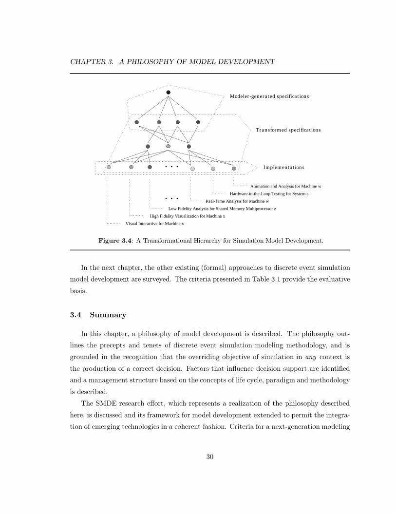
CHAPTER 3. A PHILOSOPHY OF MODEL DEVELOPMENT
. ..
...
Implementations
Transformed specifications
Visual Interactive for Machine x
High Fidelity Visualization for Machine x
Low Fidelity Analysis for Shared Memory Multiprocessor z
Real-Time Analysis for Machine w
Animation and Analysis for Machine w
Hardware-in-the-Loop Testing for System s
Modeler-generated specifications
Figure 3.4: A Transformational Hierarchy for Simulation Model Development.
In the next chapter, the other existing (formal) approaches to discrete event simulation
model development are surveyed. The criteria presented in Table 3.1 provide the evaluative
basis.
3.4 Summary
In this chapter, a philosophy of model development is described. The philosophy out-
lines the precepts and tenets of discrete event simulation modeling methodology, and is
grounded in the recognition that the overriding objective of simulation in any context is
the production of a correct decision. Factors that influence decision support are identified
and a management structure based on the concepts of life cycle, paradigm and methodology
is described.
The SMDE research effort, which represents a realization of the philosophy described
here, is discussed and its framework for model development extended to permit the integra-
tion of emerging technologies in a coherent fashion. Criteria for a next-generation modeling
30

CHAPTER 3. A PHILOSOPHY OF MODEL DEVELOPMENT
framework are identified based on the combined observations of Nance and Sargent. These
criteria serve as the evaluative basis for the approach described in this thesis.
31

Chapter 4
FORMAL APPROACHES TO DISCRETE EVENTSIMULATION
It is very easy to be blinded to the essential uselessness ofthem by the sense of achievement you get from getting themto work at all.
Douglas Adams, So Long and Thanks for All the Fish
In this chapter, the existing approaches to discrete event simulation model development
are surveyed and evaluated in terms of the requirements for a next-generation modeling
framework given in Table 3.1.1 The focus of the survey is restricted as follows: (1) only
“formal” approaches are considered since one of the criteria is to encourage automation, and
(2) programming-language-based approaches are not evaluated since the modeling method-
ological view and the philosophy described in Chapter 3 call for programming-language-
independent representations.2
4.1 Preface
When confronted with the task of analyzing a complex system, one method of recourse
is to build a model of that system. In this chapter we address a specific form of model: the
discrete event simulation model. The objective is to survey existing approaches and assess
the level of support provided for: (1) conceptualizing, (2) representing, (3) analyzing, and
(4) implementing these types of models. To preface the survey, discrete event simulation
1The CM and CS are reviewed and evaluated in Chapter 5.2For a comprehensive historical survey of simulation programming languages, see Nance [159].
32

CHAPTER 4. FORMAL APPROACHES TO DISCRETE EVENT SIMULATION
Probabilistic/Deterministic
Autonomous/Nonautonomous
PHYSICAL
STATIC
ANALYTICAL
PRESCRIPTIVE
NUMERICAL
DESCRIPTIVE
DYNAMIC
ABSTRACT
Linear/Nonlinear
Stable/Unstable
Transient/Steady State
Solution Technique
Study Objective
Temporal Nature
Model Representation
Figure 4.1: A Classification Scheme for Discrete Event Simulation (DES) Models. AllDES models fall within the class of abstract, dynamic, descriptive, numerical models.
models are placed within a broader taxonomy.
4.1.1 A model classification scheme
The art of modeling is arguably as old as mankind itself. And the uses for models, as
well as the forms that models may take, vary significantly. As a result, while the concept
of model is generally well-understood, a precise description of characteristic properties is
difficult to formulate.
The classification scheme for models adopted here is derived from [18]. Figure 4.1 illus-
trates the scope of discrete event simulation models within this scheme. The classification
scheme provides an orthoganality in four dimensions. The first dimension characterizes the
model representation. An abstract model is one in which symbols constitute the model.
A verbal or written description in English is an abstract model. A mathematical model is
described in the symbology of mathematics and is a form of abstract model. A simulation
model is built in terms of logic and mathematical equations and is considered an abstract
model. A physical model is a replica, often on a reduced scale, of the system it represents.
A physical model “looks like” the system it represents and is also called an iconic model.
The second dimension characterizes the study objective underlying the model. A de-
scriptive model describes the behavior of a system without any value judgement on the
quality of such behavior. A prescriptive (normative) model describes the behavior of a
33

CHAPTER 4. FORMAL APPROACHES TO DISCRETE EVENT SIMULATION
system in terms of the quality of such behavior. When solved, these models provide a
description of the solution as optimal, suboptimal, feasible, infeasible, and so on. Linear
programming models are prescriptive, for instance.
A third dimension relates to the presence of temporal properties in the model. A static
model is one which describes relationships that do not change with respect to time. Static
models may be abstract or physical. An architectural model of a house is a static physical
model. An equation relating the area and volume of a polygon is a static mathematical
model. A dynamic model is one which describes time-varying relationships. A wind tunnel
which shows the aerodynamic characteristics of proposed aircraft design is a dynamic phys-
ical model. The equations of motion of the planets around the sun constitute a dynamic
mathematical model.
The fourth dimension identifies a solution technique. An analytical model is one which
provides closed-form solutions using formal reasoning techniques, e.g. mathematical deduc-
tion. A numerical model is one which may be solved by applying computational procedures.
Discrete event simulation models are considered in the class of abstract, dy-namic, descriptive, numerical models.
As illustrated in Figure 4.1, within this general classification of discrete event simulation
models a subordinate classification scheme exists. Discrete event simulation models may
be defined with various combinations of the following characteristics: (1) a linear model is
one which describes relationships in linear from, and a nonlinear model describes nonlinear
relationships; (2) a stable model is one which tends to return to its initial condition after
being disturbed, while an unstable model is one which may not return to its initial condition
after being disturbed; (3) a steady-state model is one whose behavior in one time period is
of the same nature as any other time period, while a transient model is one whose behavior
changes with respect to time; (4) a probabilistic (stochastic) model is a model in which
at least one state change is a function of one or more random variables, otherwise, the
model is deterministic, and (5) an autonomous model is one in which no input is required
(or permitted) from the environment, other than at model initiation, while a model that
permits input to be received from its environment at times other than model initiation is a
nonautonomous model.
34

CHAPTER 4. FORMAL APPROACHES TO DISCRETE EVENT SIMULATION
4.1.2 Formalism and discrete event models
Approaches surveyed in this chapter are considered solely with regard to the construction
and use of models for the explicit purpose of discrete event simulation.3 These models are
referred to as discrete event simulation models, or discrete event models. The systems
underlying these models may be referred to (somewhat misleadingly) as discrete event
systems.
Discrete event models may provide a variety of means by which to understand, and
reason about, the underlying system. These provisions may range from the highly in-
tuitive to the completely mathematical. While intuitive assistance can be valuable, the
ever-increasing investment in discrete event simulation as a problem-solving technique (de-
scribed in Chapter 1) demands methods through which properties of the simulation may be
formally established. According to [212, p. 641]:
A formalism provides a set of conventions for specifying a class of objects in aprecise, unambiguous, and paradigm-free manner. The structure of a formalismfurther provides a basis for measuring the complexity of objects in that class.
Each of the surveyed approaches are formal in nature.
4.2 Lackner’s Formalism
Simulation, as a computer-based problem-solving technique, is essentially as old as the
computer itself. And like many other computer-related techniques, its use and application
preceded the development of a cogent theory. The technique of computer simulation was
driven in the earliest years by simulation program language (SPL) developments (see [159]).
But during the early 1960s, Michael Lackner became among the first to recognize, and state
unequivocally, the need for the development of a general theory of systems and models
separate from the development of SPLs. Lackner [125, pp. 25,27] observes:
What has happened in the development of simulation languages is this: the or-derly scheme of relationships has been expressed in computer code, the programsthat are a part of every model. A modeler using the language understands thatthis scheme is supplied; he does not alter the scheme in using the language;
3We examine some popular analytic techniques but only in the context of their use in simulation modeldevelopment.
35

CHAPTER 4. FORMAL APPROACHES TO DISCRETE EVENT SIMULATION
he describes system elements in accordance with the category system, which isalso invariant. The simulation language is a part of a simulation scheme that isbased on a theory of systems, but the theory has been neither elucidated nor de-veloped. . . .Only by appeal to this [general] theory [of systems] may a modelersay “this is a model of object system x” and “this is how the model behaves.”Only by such appeal may he explain why4 it is a model, and why the model sobehaves. . . .Furthermore, development of system theory should make possibledeductions of interesting measures and properties of simulation models that arenot dependent on empirical observation of the models’ [sic.] behavior.
Lackner presents a theory of discrete event systems in which change, not time, is prim-
itive; the theory, and the “Calculus of Change” require that time is defined in terms of
change. The following description is adapted from [124, 125].
4.2.1 Defining the theory
4.2.1.1 The problem
Lackner observes that the fundamental dilemma faced in simulation modeling is the
necessity of characterizing the dynamic in static terms. Whatever methods are used, limi-
tations are naturally encountered [125, p. 10]. The logical complexity of the model can be
increased by introducing conditional procedures, but two essential features of many systems
are still lacking in the program structure: (1) the asynchronous operation of related com-
ponents, and (2) the effects of varying duration of independent processes. These system
characteristics are among the most difficult to reduce to mathematical expression [125, p.
13].
4.2.1.2 System and state
According to Lackner, in a digital simulation a computer simulates an object system (the
system in the real world, or nature space, that is the subject of study) by performing an
algorithm to produce a sequence of states, internal to the computer, that may be interpreted
as describing the behavior of the object system.
A system state description can be considered to be an n-dimensional vector, where n
is equal to the number of variables contained in the system description. The variables
4Underlined in the original.
36

CHAPTER 4. FORMAL APPROACHES TO DISCRETE EVENT SIMULATION
may have arithmetic or logical values, and each member of a time series of system state
descriptions may not only contain different values of system variables but be formed of a
different set of variables; the particular variables appropriate to describing the state of the
system may differ from time to time. Thus, two kinds of changes to a state description
may be distinguished: (1) changes in the values of variables, and (2) changes in existence
of variables.
4.2.1.3 Weltansicht
Lackner [125, p. 26] gives the first characterization of conceptual frameworks. He makes
the observation that the final expression of a digital simulation model is computer code –
algorithms and data – but such a categorization of system elements does not produce a
useful model. A more restrictive set of categories is necessary to the establishment of a
general approach to modeling systems. He points out that GPSS requires that a model be
defined in terms of “transactions” which seize “stores” or “facilities” and form “queues.”
SIMSCRIPT requires a breakdown in terms of “entities, “attributes,” “sets,” and “events.”
Lackner asserts that such a restrictive set of categories is identified with a special view
or apprehension of reality as a whole, a Weltansicht, which a modeler adopts when contem-
plating an object system. “A modeler looks at the system in a certain way; certain kinds
of things are contemplated, and an orderly scheme of relationships among these kinds of
things is assumed.”
4.2.2 The Change Calculus
According to Lackner, the notion of change is implicit in the idea of system simulation:
the object system is understood to exhibit behavior. The behavior may be entirely due to
the actions of an individual agent in the system, or it may be a function of the actions of
several agents, and these agents may act sequentially or simultaneously. In the latter case,
Lackner notes that the method of modeling must take cognizance of parallel processes and
simultaneous changes [125, p. 5].
Lackner [125, p. 28] claims that the formal relations used in traditional mathematical
analysis and formal logic are most appropriate to the description of static, unchanging
situations. Change has no real place in these methods. Rules governing change are not
37

CHAPTER 4. FORMAL APPROACHES TO DISCRETE EVENT SIMULATION
expressed, but implied by equations expressing static relationships among those entities
that are affected by change. The theory on which the Change Calculus is based stipulates
that all activity is the realization of change. In Lackner’s view, entities are related to each
other by their communal “preclusion” or “evocation” of change, that is, one entity often
causes or prevents a change in another entity.
The change relation. Change is formalized as a relation, denoted by a colon (:), as a
class of antecedent-consequent pairs of logical situations. Logical situations are described
in the form of conjunctions of individual, state-descriptive sentences. Individual change
relations are written, for example, α : β and read “whenever α, then β instead,” where α
and β are conjunctions (or state descriptive variables).
A complete state description consists of the conjunction of a number of system de-
scriptive sentences. It is referred to as the system in the formalization, and the conjoined
sentences are referred to as the laws of the system.
The operation of change brings about a consequent system which is again described by
a conjunction of sentences referred to as the laws of the consequent system.5
Primitive terms. Five primitive terms are defined: (1) K, a dyadic functor, (2) W, a
dyadic change functor, (3) N, a monadic functor, (4) ∧, the null sequence, and (5) a, b, c, . . . ,
sequential variables.
Rule of definition. A new term can be introduced into the system by formulating a
group of terms, called the definition and consisting of: (1) an expression that contains the
new term and in which all the others are terms of the system; (2) the equality symbol, =;
(3) an expression that contains only primitive terms or terms already defined.
Rules of formation.
1. A variable is a consequent.
2. ∧ is a consequent.
3. A group of terms consisting of K followed by two consequents is a consequent.
5The system evolves as an evolution of consequent systems. Lackner does not formally discuss themechanism(s) by which this process may be terminated.
38

CHAPTER 4. FORMAL APPROACHES TO DISCRETE EVENT SIMULATION
4. A consequent is an antecedent.
5. A group of terms consisting of N followed by a variable is an antecedent.
6. A group of terms consisting of K followed by two antecedents is an antecedent.
7. A group of terms consisting of W followed by an antecedent followed by a consequentis a change relation.
8. A group of terms consisting of N followed by a change relation is an antecedent.
9. A change relation is a consequent.
10. A consequent is a sentence.
Definitions. WApqr = KKWKpqrWKNpqrWKpNqr
WCpqr = KKWKNpqrWKpqrWKNpNqr
WEpqr = KWCpqrWCqpr
WDpqr = KKWKpNqrWKNpqrWKNpNqr
Rules of deduction. Five rules of deduction are described.
Rules of substitution. (1) A variable or a change relation may be substituted for
a variable, but the same variable or change relation must be substituted for all equiform
occurrences of variables in the expression; (2) a sentence or antecedent consisting of a
number of K’s followed by the same number plus one of sentences or antecedents, in any
order, may be substituted for a sentence or antecedent consisting of the same number of K’s
followed by the same number plus one of sentences or antecedents each of which is equiform
with a sentence or antecedent in the expression substituted; (3) a sentence or antecedent
may be substituted for a sentence or antecedent consisting of K followed by two occurrences
of a sentence or antecedent equiform with the sentence or antecedent substituted.
Rule of substitution by definition. A definition may be substituted for the expres-
sion it defines in a sentence, and reciprocally, without being substituted for all equiform
occurrences of that expression.
Rule of detachment. If a sentence consisting of K followed by two sentences is a
law of the system, a sentence equiform with either the first or second can be posited as a
law of the system.
39

CHAPTER 4. FORMAL APPROACHES TO DISCRETE EVENT SIMULATION
Rule of conjunction. If two sentences are laws of the system, a sentence consisting
of K followed by two sentences equiform with the first two sentences may be posited as a
law of the system.
Rules of detachment of the consequent system. (1) A change relation is effective
if it is a law of the system and if its antecedent, or every antecedent that is conjoined in
its antecedent and is not itself a conjunction, is either equiform with a sentence that is a
law of the system or consists of N followed by an antecedent that is not equiform with
a law of the system; (2) a sentence equiform with the consequent of an effective change
relation must be posited as a law of the consequent system; (3) a sentence that consists of
a variable or a change relation and that is not and cannot, under the rules of substitution,
be made equiform with an antecedent conjoined in the antecedent of an effective change
relation must be posited as a law of the consequent system.
Axiom. (1) ∧
4.2.3 Examples
The example of a deduced sequence provided in [125] is reproduced here in Figure 4.2.
A less cryptic example of the Change Calculus from [124] is given in Figure 4.3. This
example describes a simple producer-consumer simulation using the following notation: (1)
Ti/j means “thing i is in state j;” (2) Ni, j means “duration time normally distributed
with mean i time units and standard deviation j time units;” (3) Pi means “duration time
is Poisson distributed with mean i time units;” (4) Ai, j means “the inclusive disjunction,
either i or j.” The syntax is:
(antecedent logical situation):(consequent logical situation) (required duration of antecedent)
For this example, Lackner stipulates: (1) given the occurrence, and specified endurance,
of an antecedent logical situation (ALS), the ALS yields to the consequent logical situation
(CLS); (2) destruction of the ALS before the required endurance precludes the occurrence
of the CLS; (3) if a duration time is not stated, duration time is assumed to be 0. All
duration time distributions are truncated: 0 < t ≤ ∞. (4) Things and states mentioned on
40

CHAPTER 4. FORMAL APPROACHES TO DISCRETE EVENT SIMULATION
ϕ0 = (x : x)(yx : y)(xy(x : x)(yx : y) : xy(x : ∧)(yx : x))ϕ1 = x(x : x)(yx : y)(xy(x : x)(yx : y) : xy(x : ∧)(yx : x))ϕ2 = y(x : x)(yx : y)(xy(x : x)(yx : y) : xy(x : ∧)(yx : x))ϕ3 = xy(x : x)(yx : y)(xy(x : x)(yx : y) : xy(x : ∧)(yx : x))ϕ4 = xy(x : ∧)(yx : x)(xy(x : x)(yx : y) : xy(x : ∧)(yx : x))ϕ5 = y(x : ∧)(yx : x)(xy(x : x)(yx : y) : xy(x : ∧)(yx : x))ϕ6 = x(x : ∧)(yx : x)(xy(x : x)(yx : y) : xy(x : ∧)(yx : x))ϕ7 = (x : ∧)(yx : x)(xy(x : x)(yx : y) : xy(x : ∧)(yx : x))
Figure 4.2: A Deduced Sequence in the Change Calculus. A sequence of state descriptionsϕ1ϕ2 . . . is produced from an original complete state description ϕ0. Notation: (p : q) =Wpq; pq = Kpq; p = Np; ϕi = complete state description i.
the ALS and not in the CLS are destroyed; (5) Things and states mentioned in the CLS
and not in the ALS are created.
4.2.4 Evaluation
An evaluation of the Change Calculus with respect to the identified requirements for a
next-generation modeling framework appears in Table 4.1. The evaluation procedure defines
four levels of support for a given requirement: (1) not recognized – no documentation
can be found which indicates that the evaluated approach considers the requirement a
desirable characteristic; (2) recognized, but not demonstrated – documentation suggests
that the requirement is recognized as important, however no mechanism is described to
support it; (3) demonstrated – at least one source can be found that indicates support for
the requirement; (4) conclusively demonstrated – substantial evidence indicates that the
requirement is supported.
Lackner’s thesis – the need to define a theory of modeling separate from the purview
of SPLs – initiates a line of modeling methodological research that has persisted for over
thirty years. This fact, alone, makes his work a significant contribution to the history of
41

CHAPTER 4. FORMAL APPROACHES TO DISCRETE EVENT SIMULATION
Thing Symbol StateApple T1 On tree (1); On ground (2); Rotten (3)Boy T2 Hungry (1); Sated (2); Leaves the scene (3)Tree T3 Producing apples (1); Not producing apples (2)
Statement CommentsT1/2T2/1 : T2/2 Given an apple on the ground and a hungry boy, the apple
disappears and the boy is sated.T2/2 : T2/1;N6, 1.5 A sated boy becomes hungry in about 6 time units.T2/1 : T2/3;N40, 15 A hungry boy leaves the scene in about 40 time units.T2/A1, 2 : T2/3;P1000 A boy leaves the scene in about 1000 time units, whether he
has been hungry or sated.T1/1 : T1/2;P20 An apple on the tree falls to the ground about 20 time units
from first appearance.T1/2 : T1/3;P3 An apple rots if it is on the ground about 3 time units.T3/1 : T1/1T3/1;P5 A tree producing apples does so at a rate of about 1 every
5 time units.T3/1 : T3/2;N18, 6 After a tree has been producing apples for about 18 time
units, it stops producing apples.T3/2 : T3/1;N18, 4 When a tree hasn’t been producing apples for about 18 time
units, it starts producing apples.
Figure 4.3: A Producer-Consumer Model in the Change Calculus.
42

CHAPTER 4. FORMAL APPROACHES TO DISCRETE EVENT SIMULATION
Table 4.1: Evaluation of the Change Calculus as a Next-Generation Modeling Framework.Level of Support is given as: 1 - Not Recognized; 2 - Recognized, but Not Demonstrated; 3- Demonstrated; 4 - Conclusively Demonstrated.
Requirement Level of SupportEncourages and facilitates the production of model and studydocumentation, particularly with regard to definitions, 2assumptions and objectives.
Permits model description to range from very high to very low level. 2Permits model fidelity to range from very high to very low level. 1Conceptual framework is unobtrusive, and/or support 2is provided for multiple conceptual frameworks.
Structures model development. Facilitates management of model 2description and fidelity levels and choice of conceptual framework.
Exhibits broad applicability. 2Model representation is independent of implementing language 3and architecture.
Encourages automation and defines environment support. 2Support provided for a broad array of model verification and 2validation techniques.
Facilitates component management and experiment design. 1
discrete event simulation, and warrants its treatment here. His calculus, however, is incom-
plete, cryptic, and difficult to use. The number of antecedent-consequent pairs will likely
become quite large for complex models, and no provisions for managing these statements
are made. Essentially, the method is reducible to a finite state automaton, a form which
may be generally more appealing, and has been adopted – in one form or another – by
several modeling approaches. Possibly as a result of this, the Change Calculus has seen no
development since the initial publishing during the early and middle 1960s.
4.3 Systems Theoretic Approaches
Several approaches and methodologies (including Lackner’s calculus) for discrete event
modeling trace their origins to general systems theory. General systems theory postulates
that real systems obey the same laws and show similar patterns of behavior even if they are
physically dissimilar [201].
The most developed appeal to general systems theory in the context of discrete event
43

CHAPTER 4. FORMAL APPROACHES TO DISCRETE EVENT SIMULATION
simulation modeling is by Zeigler [250] in his creation of the discrete event system specifi-
cation (DEVS) formalism (discussed below), and his work continues to be by far the most
prominent in this arena [250, 251, 252]. Zeigler uses the theory to establish a hierarchy of
system specifications. These are identified as: (1) system specification input-output relation
observation (IORO), (2) system specification input-output function observation (IOFO),
(3) system specification, (4) structured system specification, and (5) system specification
network. Zeigler demonstrates that specifications in his formalism may be automatically
transformed to reflect each level of the hierarchy through a collection of equivalence pre-
serving morphisms. Zeigler purports, however, that the hierarchy is independent of any
particular modeling formalism; any formalism may be employed to specify a system at any
level. Among the system formalisms Zeigler describes are differential equation system spec-
ifications (DESS), discrete time system specifications (DTSS), and discrete event system
specifications (DEVS).
4.3.1 The DEVS formalism
Zeigler [250] defines a methodology for discrete event modeling known as the discrete
event system specification (DEVS) formalism (see also [253]).
4.3.1.1 Background
DEVS – with its primary influences in general systems theory, and to a lesser extent,
mathematical systems theory, and automata theory – identifies three major conceptual ele-
ments of a discrete event simulation: (1) the system, (2) the model, and (3) the computer.6
Two relationships are also described: (1) modeling, which deals primarily with the rela-
tionship between systems and models, and (2) simulation, which refers primarily to the
relationships between models and computers.
Zeigler [250, p. 4] defines a system as, “some part of the real world, which is of interest.
The system may be natural or artificial, in existence presently or planned for the future.”
The system is a source, or potential source, of behavioral data consisting of XT plots, where
6Zeigler expands the model element to include three parts: (1) the experimental frame, which providesthe basis for model validation, (2) the base model, a valid model in all allowable experimental frames (notactually producible), and (3) the lumped model, a simpler model generated by “lumping” together and furtherabstracting the base model.
44

CHAPTER 4. FORMAL APPROACHES TO DISCRETE EVENT SIMULATION
X is some variable of interest, and T is time. A model is viewed as a set of instructions
for generating behavioral data, and a computer as a device (man or machine) capable of
producing the data from the instructions given by the model. General systems theory
provides five categories for models (in no particular order):
• Models may be classified according to their time base. In a continuous time model,time is specified to flow continuously – the model clock advances smoothly throughthe real numbers toward ever-increasing values. In a discrete time model, time flowsin jumps. The model clock advances periodically, jumping from one integer to thenext (the integers represent multiples of some specified time unit).
• A second category relates to the range sets for model descriptive variables. In adiscrete state model, variables assume a discrete set of values. A discrete event modelis a continuous time/discrete state model.7 In a continuous state model, variableranges can be represented by the real numbers (or intervals thereof). A differentialequation model is a continuous time/continuous state model.
• The third category is based on the cause-effect relationships in the model. A stochastic(probabilistic) model contains at least one random variable. In a deterministic model,no random variables appear.
• Another category relates the model to its environment. If the environment has noeffect on the model, the model is autonomous. A nonautonomous model has inputvariables whose values are not controlled by the model, but to which it must respond.
• A fifth category relates to whether the rules of interaction for a model depend ontime. A model is time invariant if the rules of interaction are independent of time.Otherwise, the model is time varying.
The two relations are elaborated as follows:
• The modeling relation deals with the validity of the model. Models may be classifiedas:
1. Replicatively valid – if the model matches data already acquired from the system.2. Predictively valid – if the model matches data prior to its being generated by
the real system.3. Structurally valid – if the model not only reproduces the observed system be-
havior, but truly reflects the way in which the real system operates to producethis behavior.
• The simulation relation concerns the faithfulness with which the computer carries outthe instructions intended by the model. The level of this faithfulness is a measure ofthe correctness of the program.
7Even though time flows continuously, state changes can occur only in discontinuous jumps. A jump canbe thought of as triggered by an event. Since time is continuous, these events can occur arbitrarily separatedfrom each other. However, no more than a finite number of events can occur in a finite interval [250, p. 22].
45

CHAPTER 4. FORMAL APPROACHES TO DISCRETE EVENT SIMULATION
Zeigler observes that one of the most important aspects of modeling, and one of the least
appreciated, is communication [250, p. 7]. And while an informal model description may
communicate the essential nature of a model, it is open to certain intrinsic problems, e.g. in-
completeness, inconsistency, and ambiguity. DEVS is an appeal to formalism in an attempt
to resolve these problems.
4.3.1.2 Model definitions
The model definitions below are predicated, in part, on the following presumptions
regarding discrete event systems [250, p. 125]:
1. A discrete event system may be simulated using a simulator that is driven by a list ofevents containing the next clock times at which components are scheduled to undergoan (internally determined) state change. This time is the hatching time of the event.
2. The hatching times of some events are predictable on the basis of the results of theoccurrence (i.e. hatching) of other events. When a hatching time is predicted, it isplaced on the events list.
3. If the next hatching time of a component cannot be predicted in advance, it will notundergo a state change until and unless such a change is caused by a state transitionof a component that has been prescheduled.
Atomic Model. An atomic model, M, is given by:
M = 〈X, S, Y, δint, δext, λ, ta〉
where
X Input events set.
S Sequential states set.
Y Output events set.
δint : S → S Internal transition function.
δext : Q×X → S External transition function.
Q = (s, e) | s ∈ S, 0 ≤ e < ta(s) (the total state of M)
λ : S → Y Output function.
ta : S →Rnonneg Time advance function.
Essentially, an atomic DEVS model is described by a set of states (S), inputs (X), outputs
(Y ), and four functions that govern the behavior of the model. An atomic model is a modular
46

CHAPTER 4. FORMAL APPROACHES TO DISCRETE EVENT SIMULATION
unit, its I/O interfaces form ports through which all environment interaction occurs. The
interior of the model is composed of state variables, and the dynamic behavior of the model
is described by two classes of events:• Input events. These lead to external event transitions, i.e. on the occurrence of an
input event, the model appeals to its external transition function for the next state.
• Time scheduled internal events. For each state the time advance function defines thetime interval to the next internal event. When this time has elapsed, an internalevent occurs, the system produces an output event and transitions to the next stateas determined by the internal transition function.
Coupled Model. In the DEVS approach, an atomic model is constructed, and by con-
necting together atomic models, coupled models may be created for complex systems. A
coupled model, DN, is given by:
DN = 〈D, Mi, Ii, Zi,j, SELECT 〉
where
D Component names set.
For each i in D (1) Mi = atomic DEVS for component i in D;
(2) Ii = set of influencees of i.
For each j in Ii Zi,j : Yi → Xj; i-to-j output translation function.
SELECT E ⊆ D → D ∀E = ∅, SELECT (E) ∈ E;
tie-breaking selector.
The specification of complex models by connecting the I/O ports of atomic models is referred
to as modular coupling. Coupled models also have their own I/O ports and may be used in
even larger coupled models, this is referred to as hierarchical modeling [191].8 From their
I/O interface, coupled models are not distinguishable from atomic components.
Praehofer and Pree [191, p. 597] observe that conventional discrete event modeling
approaches and simulation languages emphasize the concept of event, or activity, or process,
while the DEVS approach emphasizes state. Dynamic behavior is organized around the
phase variable – which denotes global system state. Depending on the current phase of the
system, it will react differently to external inputs and the occurrence of internal events. In
DEVS modeling, the phase actually defines a partition of the state space of the model.
8See Section 4.10.1 for a more detailed characterization of hierarchical modeling.
47

CHAPTER 4. FORMAL APPROACHES TO DISCRETE EVENT SIMULATION
4.3.1.3 DEVS-based approaches
The basic tenet of general systems theory – that all systems can be described in common
terms – leads naturally to the application of the DEVS approach to areas outside discrete
event simulation. A substantial proportion of ongoing DEVS-related research addresses
modeling issues in areas such as artificial intelligence, continuous and combined simulation;
very little of what could be described as pure discrete event simulation research is evident.
Zeigler et al. [254] describe DEVS-Scheme. Built on PC-Scheme, a Lisp dialect and
object-oriented programming subsystem for microcomputers, DEVS-Scheme exists in four
layers:
1. The Lisp-based object-oriented foundation that provides processing capabilities andenvironment support.
2. A systems model specification layer that provides systems theoretic basis and modelspecification language.
3. A systems entity structure/model base layer that provides axiomatic specification andmodel synthesis (see Section 4.3.2).
4. A systems design layer called the frames and rules associated system (FRASES), thatembeds the system entity structure in a frame-based knowledge representation scheme.
According to Kim [118, p. 401], the DEVS-Scheme approach supports building models
in a hierarchical, modular manner: “a systems oriented approach not possible in conven-
tional languages.” Sevinc [213] describes DEVS-CLOS, a close relative of DEVS-Scheme,
but based on the Common Lisp Object System. Another object-oriented approach is DE-
VSIM ++, an object-oriented simulation environment built on C ++ [119].
Praehofer and Pree [191] extend the DEVS formalism to facilitate combined, discrete
event and continuous multiformalism modeling (also referred to as multimodeling) in an
approach called DEVandDESS.
Thomas [227] describes the Hierarchical Object Nets (HON) approach. HON is pur-
ported as an open visual object-oriented modeling and simulation system. Based on DEVS
and implemented in C ++, HON is designed to support only discrete event simulation.
Thomas observes [227, p. 651]:
The [DEVS] formalism provides a basis for extending the view on models, allowshandling them as knowledge used to answer a multiplicity of questions ratherthan as “just simulation models.” However, when applied only to simulation
48

CHAPTER 4. FORMAL APPROACHES TO DISCRETE EVENT SIMULATION
problems the flexibility becomes a problem. This affects the ease-of-use of aDEVS-based simulation system and its simulation efficiency. We propose HONas a modification of DEVS in order to extend the formalism’s practicability tomake this powerful means available to practice.
This recognition is also made by Zeigler et al. [254, p. 85] as a basis for DEVS-Scheme: “As
a set theoretic concept, the DEVS formalism by itself is not a practical means of specifying
models.”
4.3.2 System entity structure
According to Cellier et al. [45, p. 60], the system entity structure (SES) is a mechanism
to describe hierarchically structured sets of objects and their interrelations. The SES is a
labeled tree with attached variables types, i.e. a graphical object that describes the decom-
positions of systems into parts. A knowledge representation scheme, SES formalizes the
modeling of systems in terms of decomposition, taxonomic and coupling relationships. SES
provides a formal description of how physical objects are decomposed into parts.
Rozenblit and Zeigler [201] describe a methodology based on SES called the knowledge-
based simulation design (KBSD) methodology. KBSD focuses on the use of modeling and
simulation techniques to build and evaluate models of systems being designed. KBSD
treats the design process as a series of activities that comprise specification of design levels
in a hierarchical manner (decomposition), classification of system components into different
variants (specialization), selection of components from specializations and decompositions,
development of design models, experimentation and evaluation by simulation, and choice
of design solutions. SES is used to capture the decomposition, taxonomy, and coupling
relationships. By a process called pruning, the SES can be converted into a DEVS.
4.3.3 Evaluation
Evaluation of the systems theoretic approaches with regard to the identified requirements
for a next-generation modeling framework appears in Table 4.2. The evaluation indicates
that the theoretical basis provided by general systems theory is both sound and powerful.
Zeigler’s theory has been demonstrated applicable to a wide variety of problem domains, as
well as for solution techniques other than strictly discrete event simulation. The formalisms
(DEVS, SES) provide a well-defined manner through which to structure model development.
49

CHAPTER 4. FORMAL APPROACHES TO DISCRETE EVENT SIMULATION
Table 4.2: Evaluation of Systems Theoretic Approaches as a Next-Generation ModelingFramework. Level of Support is given as: 1 - Not Recognized; 2 - Recognized, but NotDemonstrated; 3 - Demonstrated; 4 - Conclusively Demonstrated.
Requirement Level of SupportEncourages and facilitates the production of model and studydocumentation, particularly with regard to definitions, 2assumptions and objectives.
Permits model description to range from very high to very low level. 2Permits model fidelity to range from very high to very low level. 2Conceptual framework is unobtrusive, and/or support 1is provided for multiple conceptual frameworks.
Structures model development. Facilitates management of model 3description and fidelity levels and choice of conceptual framework.
Exhibits broad applicability. 4Model representation is independent of implementing language 3and architecture.
Encourages automation and defines environment support. 3Support provided for a broad array of model verification and 3validation techniques.
Facilitates component management and experiment design. 4
This framework should enhance the model verification and validation problem as well as
contributing to the automatability of approach. Furthermore, Zeigler’s identification of an
experimental frame stresses the recognition of a context for any modeling effort.
While the methodology is sound, these approaches suffer from a lack of representational
expressiveness. The existing literature regarding the DEVS-based approaches and the SES
fails to demonstrate either an unobtrusive conceptual framework or the ability to describe
system behavior at anything other than a low level. Still, such capabilities seemingly could
be incorporated within an approach based on general systems theory.
4.4 Activity Cycle Diagrams
Tocher [229] introduces a notation for describing the logical “flow” of a simulation.
These flow diagrams represent one of the earliest attempts to provide a graphical descrip-
tion of a simulation model, however they are essentially flowcharts and fail to exploit the
narrowed focus provided by the context of discrete event simulation. Possibly, it was this
50

CHAPTER 4. FORMAL APPROACHES TO DISCRETE EVENT SIMULATION
recognition that led to the development of a notation called “wheel charts” [230]. The wheel
chart notation evolved further into a form known as activity cycle diagrams (or entity cycle
diagrams) first described in [101]. These diagrams have become an integral part of much of
the simulation work in the activity scan and three-phase arenas that has persisted, largely
in the UK, since the late 1960s.
In the typical activity cycle diagram (ACD) based approach, a simulation model is
viewed as a collection of interacting entities. An entity is any component of the model which
can be imagined to retain its identity through time. Entities are either idle – in notional or
real queues, or active – engaged with other entities in time consuming activities. An active
state usually involves the cooperation of different entities. A passive state, or queueing state,
involves no cooperation between different entities and is generally a state in which the entity
waits for something to happen. The duration of an activity can always be determined in
advance, whereas the duration of the queueing state cannot be so determined [188]. The
symbology for ACDs is minimal, with one symbol each for a queue and an activity as shown
below.
queue activity
To specify a model using ACDs, a life cycle, or activity cycle, composed of queues and
activities must be given for each class of entity in the model. A common restriction is that
queues and activities must alternate in the representation. If necessary, dummy queues may
be incorporated into the diagram. Typically each activity cycle must be closed.
4.4.1 Example
The quintessential ACD example is the English Pub. The model contains three entities:
a man, a barmaid, and a glass.9 The behavior of each entity is fairly simple. The man either
drinks or waits to drink. The barmaid either pours a drink or is idle. The glass is either
used to drink from, empty, poured into by the barmaid, or full waiting to be consumed.
The ACD for the English Pub model is given in Figure 4.4.
9The English, to their credit, have no use for political correctness.
51

CHAPTER 4. FORMAL APPROACHES TO DISCRETE EVENT SIMULATION
empty
full
drink pourwait idleGlass
BarmaidMan
Figure 4.4: Activity Cycle Diagram for English Pub Model.
4.4.2 The simulation program generator approach
The main usage of ACDs is as a front-end for simulation program generators. A program
generator is a program that produces another program in a high-level language from a simple
input description [54]. The first program generator was the Programming by Questionnaire
(PBQ) system developed at RAND [176, 177] which generated Job Shop simulations based
on information provided by a modeler via machine-readable responses to a questionnaire.
A simulation program generator is an interactive software tool that translates the logic
of a model described in a relatively general symbolism, usually ACDs, into the code of a
simulation language and so enables a computer to mimic model behavior [143]. According
to Mathewson [142], the steps in the use of a simulation program generator are to:
1. Prepare a symbolic description of the model.
2. Use the program generator to obtain a translation of the symbolic description into asimulation program.
3. Edit the simulation program to insert further detail whose representation is outsidethe scope of the symbolic logic.
Most of the work in simulation program generators has been conducted in Europe. Many
of these generators, for example CAPS/ECSL [54], DRAFT [141], and GASSNOL [236], a
simulation program generator based on the Network Oriented CAD Input Language (NO-
CADIL), are application specific and adopt the activity scan conceptual framework.
52
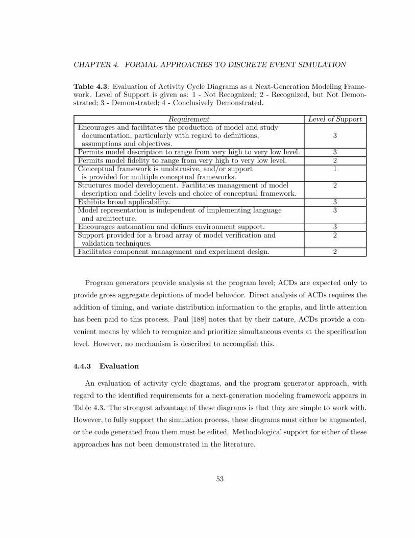
CHAPTER 4. FORMAL APPROACHES TO DISCRETE EVENT SIMULATION
Table 4.3: Evaluation of Activity Cycle Diagrams as a Next-Generation Modeling Frame-work. Level of Support is given as: 1 - Not Recognized; 2 - Recognized, but Not Demon-strated; 3 - Demonstrated; 4 - Conclusively Demonstrated.
Requirement Level of SupportEncourages and facilitates the production of model and studydocumentation, particularly with regard to definitions, 3assumptions and objectives.
Permits model description to range from very high to very low level. 3Permits model fidelity to range from very high to very low level. 2Conceptual framework is unobtrusive, and/or support 1is provided for multiple conceptual frameworks.
Structures model development. Facilitates management of model 2description and fidelity levels and choice of conceptual framework.
Exhibits broad applicability. 3Model representation is independent of implementing language 3and architecture.
Encourages automation and defines environment support. 3Support provided for a broad array of model verification and 2validation techniques.
Facilitates component management and experiment design. 2
Program generators provide analysis at the program level; ACDs are expected only to
provide gross aggregate depictions of model behavior. Direct analysis of ACDs requires the
addition of timing, and variate distribution information to the graphs, and little attention
has been paid to this process. Paul [188] notes that by their nature, ACDs provide a con-
venient means by which to recognize and prioritize simultaneous events at the specification
level. However, no mechanism is described to accomplish this.
4.4.3 Evaluation
An evaluation of activity cycle diagrams, and the program generator approach, with
regard to the identified requirements for a next-generation modeling framework appears in
Table 4.3. The strongest advantage of these diagrams is that they are simple to work with.
However, to fully support the simulation process, these diagrams must either be augmented,
or the code generated from them must be edited. Methodological support for either of these
approaches has not been demonstrated in the literature.
53

CHAPTER 4. FORMAL APPROACHES TO DISCRETE EVENT SIMULATION
4.5 Event-Oriented Graphical Techniques
4.5.1 Event graphs
Observing that graphical modeling techniques had been developed for discrete event
simulations adopting either an activity scan (activity cycle diagrams) or process interaction
(GPSS block diagrams) view, but that no such tool was available for event scheduling
models, Schruben [207] introduces a formalism dubbed the event graph.10 Using Schruben’s
terminology, the crucial elements of a discrete event simulation are state variables that
describe the state of the system, events that alter the values of state variables, and the
logical and temporal relationships among events. An event graph is a directed graph that
depicts the interrelation of the events in an event scheduling discrete event simulation. To
construct an event graph, events are defined and numbered, and represented as vertices in
the digraph. Event vertices are connected by directed edges that indicate how one event
influences the occurrence of another event.11 Two classes of edges are defined: a solid edge
represents the scheduling of an event; a dashed edge represents an event cancellation. Thus,
j k
t (i)
indicates that t time units after the occurrence of event j, event k will be scheduled to occur
provided that condition (i) holds at the time event j occurs. And,
j k
t (i)
indicates that t time units after the occurrence of event j, any currently scheduled occurrence
of event k will be canceled provided condition (i) holds at the time event j occurs.12
Some additional properties of event graphs are: (1) two vertices may be joined by
10GPSS block diagrams (see [90]) are tailored to support the transaction flow conceptual framework ofGPSS, and are not directly applicable for model development under the common process interaction worldview (e.g. as supported by SIMULA). For this reason, GPSS block diagrams are considered implementation-language-dependent, and are therefore not included in this survey.
11In the usual parlence of graph theory (see [35]) vertices in an undirected graph are connected by edges,and vertices in a directed graph are connected by arcs. The terminology applied in this chapter adheres tothat of the individual techniques, and not necessarily to the standards of graph theory.
12Schruben [207, p. 958] notes that event canceling is generally convenient in modeling but not necessary.
54

CHAPTER 4. FORMAL APPROACHES TO DISCRETE EVENT SIMULATION
more than one edge, and loops are also permitted; (2) edges without condition labels are
referred to as unconditional edges; (3) both edge delay times and condition labels may
invoke random variates; (4) event vertices and condition labels may be parameterized to
simplify the graph; (5) an event graph is not necessarily connected. Note that system time
and the list of scheduled event occurrences are implicit in an event graph.
Example. The following Parts Model example is from [207]. In this example, parts arrive
for processing by one of three identical machines. A machine is selected at random from
the set, A, of available machines. Processing may be interrupted, and parts that have their
processing interrupted will be finished once their machine resumes operation. We define:
ta = random time between part arrivalstc = cycle time required for a machine to process a parttd = random duration processing interruptionti = random interval between machine interruptionsT (j) = processing time remaining for part currently on machine j
T (j) = 0 if machine j is idleM(j) = 1 if machine j is available; 0 otherwisep = number of parts waiting for processing(i) = parts are waiting, (p > 0)(ii) = at least one machine is available, (A = ∅)τi = the time until the next currently scheduled occurrence of event ievent 1 = part arrival
p = p + 1, randomly select j ∈ A, generate taevent 2(j) = begin processing on machine j
M(j) = 0, p = p− 1, T (j) = tc −min(tc, τ4(j))event 3(j) = end processing on machine j
M(j) = 1event 4(j) = interrupt machine j
M(j) = 0, generate tdevent 5(j) = machine j return to operation
generate ti
The event graph for this model is given in Figure 4.5.
Methodology and analysis. Schruben [207, p. 960] provides little guidance in terms
of a methodology for graph construction, noting only that state variable definition, event
definition, and edge conditioning usually proceed simultaneously in developing an event
graph. Subsequent development yielded the Simulation Graphical Modeling and Analysis
(SIGMA) environment. Written in C, and using the HOOPS object-oriented picture system,
55

CHAPTER 4. FORMAL APPROACHES TO DISCRETE EVENT SIMULATION
T(j)
1
2(j)
3(j) 4(j)
5(j)
t
titdtc
(ii)
(i)
a
Figure 4.5: Event Graph for Parts Model.
SIGMA models – in the form of event graphs – are constructed and either directly executed
or automatically transformed into standard C or Pascal code [208, 209, 210]. SIGMA is
proposed as a learning environment rather than a commercial one. The environment is
somewhat limited. For example, the first vertex created during the modeling process must
always represent initialization, and editing of the source code and library routines is required
to utilize multiple random number streams. A more significant limitation is the absence
of methodological guidance in terms of defining and ordering the classes of decisions which
need to be made during model development.
Diagnostic analysis of event graph models may aid in the following [207]:
• Identifying needed state variables.
• Determining a minimal set of events that must be scheduled at model initiation.
• Anticipating logic errors due to simultaneously scheduled events.
• Eliminating unnecessary event routines.
Schruben suggests heuristics for each of these, although no attempt is made to formalize
the approach to model diagnosis.
Since 1983, several variations of event graphs have been proposed [104, 126, 189, 203],
however the work of Schruben remains the most prominent. Schruben [209] illustrates how
event graphs can be marked in a manner similar to Petri nets. In a marked event graph, the
56

CHAPTER 4. FORMAL APPROACHES TO DISCRETE EVENT SIMULATION
number of tokens in an event vertex represents the number of outstanding instances of that
event. Som and Sargent [219] formalize the analytic heuristics suggested by Schruben. Event
execution order prioritization permits the generation of an expanded event graph. From this
graph, super events are identified and used as a basis for computation, thereby reducing
event list processing and fostering more efficient implementation of event scheduling models.
Some questions exist regarding their approach, however. Yucesan [244, p. 34] gives an
example graph for which these “event reduction” rules are invalid.
4.5.2 Simulation graphs and simulation graph models
Yucesan [244] demonstrates that event graphs of some simple queueing systems are
planar, and shows that the dual of an event graph represents a model specification reflecting
an activity scan world view (see [211]). These results illustrate the possible generality of
event graphs; as a result, Yucesan [244] defines a simulation graph, which is a variant of
event graph but intended as a world-view-independent representational mechanism. The
discussion of simulation graphs given here is adapted from [246].
A simulation graph is defined as an ordered quadruple:
G = (V (G), Es(G), Ec(G),ΨG)
where
V (G) is the set of event vertices
Es(G) is the set of scheduling edges
Ec(G) is the set of canceling edges
ΨG is the incidence function
The data defined in the graph are given by the following indexed sets:
• F = fv : STATES → STATES | v ∈ V (G). The set of state transition functionsassociated with vertex v.
• C = Ce : STATES → 0, 1 | e ∈ Es(G) ∪Ec(G) The set of edge conditions.
• T = te : STATES→R+ | e ∈ Es(G) The set of edge delay times.
• Γ = γe : STATES→ R+ | e ∈ Es(G) The set of event execution priorities.
57

CHAPTER 4. FORMAL APPROACHES TO DISCRETE EVENT SIMULATION
Where STATES is defined as in Zeigler’s [250] development. A simulation graph model
(SGM) is:
S = (F , C, T ,Γ, G)
The first four sets in the above five-tuple define the entities in a model. The role played
by a simulation graph, G, in the definition of a simulation graph model, S, is analogous
to the role of the incidence function, Ψ, in the definition of a directed graph: it organizes
these sets of entities into a meaningful simulation model specification, i.e. G specifies the
relationship between the elements in the sets F , C, T and Γ [212].
4.5.2.1 Equivalence analysis
Yucesan and Schruben [246] utilize simulation graphs as a basis for evaluating the equiv-
alence of simulation model specifications. The objective is to identify when two simulation
models can be used interchangeably without actually having to run both simulations under
all possible experimental conditions and compare their output behavior. The authors’ dis-
cussion is predicated on the following definitions. In an SGM, an edge condition is simple
if it consists of two arithmetic expressions connected by a relational operator, i.e. a simple
edge condition is a relation. An edge condition is compound if it consists of two or more
relations joined by Boolean operators. A vertex is simple if there is at most one state vari-
able change associated with it. Otherwise the vertex is compound. A vertex with no state
variable changes is the identity vertex. An SGM is an elementary simulation graph model
(ESGM) if it contains only simple vertices and simple edge conditions.
Given any SGM, an associated ESGM can always be constructed by expansion of the
SGM. Expansion involves replacing all instances of single event vertices with m (m ≥ 1)
state variable changes, by m vertices in series, each with a single state variable change, and
replacing all instances of edges with compound conditions by a group of identity vertices,
each connected by edges with simple conditions. During this process, the logical structure
of the original model is always preserved [246, p. 87]. Application of the expansion rules
does not generate a unique ESGM. However, all ESGMs constructed in this manner are
mutually isomorphic and therefore form an equivalence class. The isomorphism problem is
intractable for general graphs, but efficient algorithms for planarity testing and determining
isomorphism on planar graphs do exist [105, 106].
58

CHAPTER 4. FORMAL APPROACHES TO DISCRETE EVENT SIMULATION
According to [246] SGMs S1 and S2 are structurally equivalent if they have ESGMs,
SE1 , SE2 , respectively, which are isomorphic. A further result is that structural equivalence
implies behavioral equivalence. This result is important since it means that we can a
priori analyze two model specifications to determine their equivalence, without having to
generate and run implementations of them. However, these analytic techniques have not
been implemented in an environment, so their application to large-scale models remains the
subject of future study.
Note that Overstreet [178] also shows that structural equivalence of a Condition Speci-
fication implies external equivalence. Furthermore, since digraphs utilized within the Con-
dition Specification may not be planar, he argues that no polynomial-time algorithm exists
to determine the structural equivalence of two CSs.
4.5.2.2 Complexity analysis
In [212] simulation graphs are used as a basis for analyzing model complexity. Their
focus is on complexity measures that relate directly to the structural properties of simu-
lation model specifications, with primary attention paid to predicting implementation and
maintenance costs. They define three measures of space complexity:
C1 = | V (G) |
C1 relates complexity to the size of the specification.
C2 =| E(G) || V (G) |
where E(G) = Es(G)∪Ec(G). C2 relates complexity to the number of possible component
interactions.
C3 =∑
v∈V (G)
C(v) +∑
v,w∈V (G)
I(v, w)
where C(v) denotes some measure of the complexity of vertex v, and I(v, w) denotes some
measure of interaction between vertices v and w. C3 represents the sum of the complex-
ities of each “module” and the intermodular interaction. This metric is somewhat vague,
however, since no clear choices for C(v) and I(v, w) exist.
Schruben and Yucesan [212] present a fourth complexity measure associated with the
number of control paths through a graph. Based on McCabe’s [146] work, the cyclomatic
59

CHAPTER 4. FORMAL APPROACHES TO DISCRETE EVENT SIMULATION
number of a simulation graph, G, with n vertices, e edges, and p connected components is:
η(G) = e− n + p
The results of their analysis using the four complexity measures indicate that the com-
plexity of individual events, measured as the number of modified state variables within
that event, plays a principal role in determining the execution time of a single run. The
branching structure, as measured by the cyclomatic complexity of the graph, has secondary
influence [212].13
4.5.2.3 Theoretical limits of structural analysis
Yucesan and Jacobsen [245] discuss some theoretical limitations of structural analysis.
Based on their experience with simulation graphs, the authors demonstrate that the follow-
ing properties of discrete event simulation models are intractable (albeit decidable) decision
problems:
• Accessibility of states - determining whether or not any given model state will occurduring an execution of the model.
• Ordering of events - determining the existence of, or ruling out the possibility for,simultaneous events.
• Ambiguity of model implementations - determining whether the model implementation“satisfies” the model specification.
• Execution stalling - determining whether an execution can enter a state in which nodetermined events exist and the termination condition is not met.
They further argue that these properties hold for any model representation form.14 Over-
street’s [178] conclusions, based on Turing machine analysis of the CS, are slightly different.
By reducing these issues to the Halting Problem, Turing analysis indicates that these prob-
lems are undecidable.
13The authors claim that this contradicts both Overstreet’s and McCabe’s assertions that complexitydepends only on the decision structure (branching) of a program and not on the number of functionalstatements. However, Overstreet describes conceptual complexity, not run-time complexity.
14These results seem to contradict those of Yucesan and Schruben [246] that planar graph representationsof simulation models do portend tractable analysis.
60

CHAPTER 4. FORMAL APPROACHES TO DISCRETE EVENT SIMULATION
Table 4.4: Evaluation of Event-Oriented Approaches as a Next-Generation ModelingFramework. Level of Support is given as: 1 - Not Recognized; 2 - Recognized, but NotDemonstrated; 3 - Demonstrated; 4 - Conclusively Demonstrated.
Requirement Level of SupportEncourages and facilitates the production of model and studydocumentation, particularly with regard to definitions, 2assumptions and objectives.
Permits model description to range from very high to very low level. 3Permits model fidelity to range from very high to very low level. 3Conceptual framework is unobtrusive, and/or support 2is provided for multiple conceptual frameworks.
Structures model development. Facilitates management of model 2description and fidelity levels and choice of conceptual framework.
Exhibits broad applicability. 2Model representation is independent of implementing language 3and architecture.
Encourages automation and defines environment support. 3Support provided for a broad array of model verification and 3validation techniques.
Facilitates component management and experiment design. 3
4.5.3 Evaluation
Evaluation of event-oriented approaches based on the identified requirements for a next-
generation modeling framework appears in Table 4.4. Event Graphs and Simulation Graphs
have been well-exercised over the past ten years. While the notation seems expressive and
extensible, no methodology for graph construction has been described. Experience with
SIGMA may yield results in this area.
4.6 Petri Net Approaches
According to Peterson [190], a Petri net is an abstract formal model of information flow.
Named for Carl Petri, the major use of Petri nets has been the modeling of systems which
exhibit concurrency. This most common use is motivated by a desire to analyze this class of
systems – by modeling them as Petri nets, and then manipulating the Petri nets to derive
properties of the modeled systems. As a result, much study has gone into the development
of techniques for analyzing Petri nets. One method of analysis is simulation. Petri nets
61

CHAPTER 4. FORMAL APPROACHES TO DISCRETE EVENT SIMULATION
are also, themselves, a modeling tool. They have been suggested as a formalism to model
general systems for the purpose of discrete event simulation. Petri nets are suitable for
modeling systems that can be viewed as a set of events and a set of conditions, and the
relationships among these sets [190, p. 288].
Thus the relationship between Petri nets and DES is somewhat symbiotic: Petri nets
are used to develop DES models, and DES is used to simulate Petri nets when the limits of
analytic techniques are exceeded. The use of Petri nets as a formalism for the development
of discrete event simulation models of general systems is of primary interest here.
The presentation begins with a discussion of the basic, or ordinary, Petri net. Some
common extensions to Petri nets are discussed subsequently.
4.6.1 Definitions
A Petri net is a directed bipartite graph. The graph contains two types of nodes: places
– typically represented by circles, and transitions – typically represented by bars. An arc in
the graph may exist only between places and transitions. In an ordinary Petri net, multiple
arcs between any two nodes are not allowed.
If an arc from a place P to a transition T exists, then P is called an input place of
transition T, and T is called an output transition of place P. Similar definitions hold for
output place and input transition.
At any moment, a place may have 0 or more tokens. Tokens are represented by black
dots in place nodes. A Petri net with tokens is called a marked Petri net. The distribution
of (all) tokens (to places) in a marked Petri net is called its marking.
A Petri net for a single server queueing system is given in Figure 4.6. The graph contains
three places and three transitions. The graph marking indicates that the server is idle and
no customers are waiting. A valuable feature of Petri nets is their ability to model a system
hierarchically. An entire net may be represented by a single place or transition for modeling
at a more abstract level (abstraction), or places and transitions may be expanded into
subnets to provide more detailed modeling (refinement). For example, the service transition
in the Petri net given in Figure 4.6 could be expanded into a “service starts” transition,
a “customer obtains service” place, and a “service ends” transition. Note that the graph
of Figure 4.6 does not contain any timing information, and so is not directly suitable for
62

CHAPTER 4. FORMAL APPROACHES TO DISCRETE EVENT SIMULATION
Server Idle
Customer
Service
CustomerArrives
Customer
Customer Leaves
Ready to Leave
Waiting
Figure 4.6: A Petri Net for a Single Server Queue. The marking indicates that the serveris idle and no customers are waiting.
discrete event simulation, the incorporation of time within a Petri net is discussed below.
A transition node is said to be ready if and only if there exists at least one token in
each of its input places. At any moment, 0 or more ready transitions are chosen (nondeter-
ministically) to fire. When a transition fires, its associated input tokens are removed and
new tokens are placed in each of its output places. In an ordinary Petri net, the firing of a
transition is instantaneous. Two transitions are said to be neighbors if they share at least
one input place.
While nondeterminism is potentially advantageous from a modeling point of view, it
introduces complexity into the analysis of Petri nets. However, Peterson [190, p. 229]
notes that if instantaneous firing of transitions, and a real-valued clock are assumed, the
probability of simultaneous events (transitions) goes to zero.
A net is said to be k-bounded for some integer k if no more that k tokens can be in any
place at the same time. A 1-bounded Petri net is called a safe net.
A Petri net is conservative if the number of tokens in the net is conserved.
A transition is dead in a marking if there is no sequence of transition firings that can
enable it. A transition is potentially firable if there exists some sequence that enables it. A
63
CHAPTER 4. FORMAL APPROACHES TO DISCRETE EVENT SIMULATION
transition is live if it is potentially firable in all reachable markings (defined below).
Petri net analysis. Almost all Petri net analytic techniques include the construction
of a reachability tree [190, p. 240]. In a reachability tree the nodes represent markings
of the Petri net and the arcs represent possible changes in state resulting from the firing
of transitions. Tree construction is made finite (even though the reachability set may be
infinite) through a parameterization process. Using this technique, one may determine if a
marking, say, m′ is reachable from some other marking, m.
Common Petri net analysis procedures include analysis for (1) boundedness, (2) con-
servation, (3) coverability, and (4) reachability. The reachability problem for Petri nets,
however, has been shown to be decidable, but intractable [190, p. 249].
Petri nets that allow multiple arcs are often called generalized Petri nets. Addition
of the provision for inhibitor arcs – arcs which indicate that a transition may fire only if
the corresponding place has zero tokens in it – yields a formalism equivalent to a Turing
machine [190, p. 246]. Commonly, most references to “Petri nets” refer to generalized Petri
nets with inhibitor arcs. A discussion of some special extensions and applications of Petri
nets follows.
4.6.2 Timed Petri nets
The basic Petri net definition contains no information regarding the temporal properties
of the model behavior. Timing information may be added to an ordinary Petri net to
produce a Timed Petri net in the following manner:
• Time may be associated with transitions. Each transition T has a time, δ, called theexecution time of T. The usual interpretation of this construct is that if T begins firingat time t, the input token(s) are removed at t and the output token(s) appear at timet+ δ.
• Time may be associated with places. Each place P has an associated time, δ. In thiscase, if a token appears in in P at time t, then any associated output transition maynot fire until time t+ δ.
Time may be associated with transitions only – the most common version of Timed Petri
nets [173, 197, 233], places only [6, 57], or both transitions and places [123].
64

CHAPTER 4. FORMAL APPROACHES TO DISCRETE EVENT SIMULATION
4.6.3 Stochastic Petri nets
Molloy [149] describes a stochastic Petri net (SPN) as a generalized Timed Petri net in
which the time specifications are introduced by associating exponentially distributed firing
times on transitions. Balbo and Chiola [14] present a tool, GreatSPN, which provides the
facilities to build, analyze, execute and animate SPNs.
4.6.4 Simulation nets
Torn [233, 234] describes an approach to discrete event simulation known as the simu-
lation net.15 A simulation net is an extension to the ordinary Petri net which includes:
• generalized Petri net semantics
• inhibitor arcs
• general test arcs
• temporal properties for transitions
• a notation for representing queues
According to [233] the Petri net properties important for simulation are liveness and safe-
ness. Torn [234] describes a tool, SimNet, which directly executes simulation net simula-
tions. Implemented in SIMULA, SimNet provides, among other features, the automatic
collection of common performance measures for queueing systems.
4.6.5 Petri nets and parallel simulation
Not surprisingly, due to the relationship between Petri nets and concurrent systems
(see [197]), the use of Petri nets as a basis for parallel simulation has received significant
attention.
Kumar and Harous [123] describe an approach for the parallel discrete event simulation
of Timed Petri nets based on a conservative protocol in which deadlock avoidance is im-
plemented through a variant of the null message scheme. Nicol and Roy [173] demonstrate
a method for locating and exploiting “lookahead” in a conservative parallel simulation of
Timed Petri nets. They describe an X-windows based graphical tool, pntool, which may
15Torn originally calls these structures simulation graphs.
65

CHAPTER 4. FORMAL APPROACHES TO DISCRETE EVENT SIMULATION
Table 4.5: Evaluation of Petri Net-Based Approaches as a Next-Generation ModelingFramework. Level of Support is given as: 1 - Not Recognized; 2 - Recognized, but NotDemonstrated; 3 - Demonstrated; 4 - Conclusively Demonstrated.
Requirement Level of SupportEncourages and facilitates the production of model and studydocumentation, particularly with regard to definitions, 1assumptions and objectives.
Permits model description to range from very high to very low level. 1Permits model fidelity to range from very high to very low level. 3Conceptual framework is unobtrusive, and/or support 1is provided for multiple conceptual frameworks.
Structures model development. Facilitates management of model 2description and fidelity levels and choice of conceptual framework.
Exhibits broad applicability. 3Model representation is independent of implementing language 3and architecture.
Encourages automation and defines environment support. 3Support provided for a broad array of model verification and 3validation techniques.
Facilitates component management and experiment design. 1
be used to develop Timed Petri net models for the YAWNS simulation environment [174].
Another method, known as the transition firing protocol is described in [228].
4.6.6 Evaluation
Evaluation of Petri net-based approaches with respect to the identified requirements for
a next-generation modeling framework appears in Table 4.5. Petri nets provide a simple
mechanism for the representation of system behavior. However, the conceptual framework
seems too restrictive, and no provisions have been demonstrated for model definitions,
assumptions and objectives. Nor has a higher-level representation been identified. Very
little work is evident regarding the use of Petri nets within the context of an end-to-end
simulation study.
66

CHAPTER 4. FORMAL APPROACHES TO DISCRETE EVENT SIMULATION
4.7 Logic-Based Approaches
Simulation model development approaches that provide a basis for formally reasoning
about discrete event simulations (at the model specification level) are investigated in this
section. Proof of correctness dates to [68], and a great deal of literature in exists in the area
of computational logics: in artificial intelligence, software engineering, as well as philoso-
phy. A body of research concerning the application of logic programming to discrete event
simulation has evolved, but the focus of these efforts is mostly at the implementation level,
and so are not examined in this survey. Perhaps the most extensive application of logics in
computer science has been in the arena of real time systems (see [196] for a brief discussion).
These real time, and temporal logics may be suitable for developing discrete event simula-
tion models. However, the efforts along these lines are highly embryonic, and any potential
benefits are speculative. For this reason, and for space considerations, a discussion of real
time and temporal logics is considered beyond the scope of this survey.
4.7.1 Modal discrete event logic
By far the most developed effort in this area is due to Radiya and Sargent [195, 196].
According to [196, p. 4], Zeigler’s systems theoretic work is the major theoretical founda-
tion for discrete event modeling and simulation (DEMS). Radiya and Sargent suggest their
own efforts, as well as Glynn’s [87, 88] work in generalized semi-Markov processes as pos-
sible alternatives for a theoretical DEMS foundation [196, p. 4]. The authors identify the
contributions of their work as follows:
• Identification of important semantic concepts, starting with the two fundamental con-cepts of instantaneous propositions (events) and interim variables (similar to piecewiseconstant state variables) and culminating in the central concept of discrete event (DE)structure.
• A modal discrete event logic, LDE , for expressing discrete event models. The logicLDE is defined, independent of its simulation procedures, by specifying its syntax andsemantics with respect to DE structures. In LDE a model of a system is a set offormulae. The purpose of the semantics is to specify conditions under which a DEstructure can be said to “satisfy” a model in LDE . A DE structure satisfies a modelif the truth values of instantaneous propositions and changes in the values of interimvariables at every instant of the DE structure are completely accounted for by themodel.
67

CHAPTER 4. FORMAL APPROACHES TO DISCRETE EVENT SIMULATION
• A simulation procedure for simulating models expressible in a sublogic of LDE. Simu-lation is defined to be a process of finding a DE structure that satisfies a given model,and a simulation procedure is an algorithm that defines this process.
Semantic concepts. An instantaneous proposition is a proposition such that: (1) its
truth (occurrence) can be claimed at any instant, and (2) over any bounded interval, the
proposition true (occurs) only at finitely many instants. Used to represent events, this
differs from Nance’s [156] characterization. An event, as defined by Radiya, is not directly
associated with instants or state changes. An occurrence of an event is associated with
an instant but not necessarily a state change. In a queueing network example suggested
by [196, p. 10], neither instants nor state changes are associated with an event “customer
arrival,” but its occurrence must be associated with an instant. Also certain occurrences of
“customer arrival” may not be associated with state changes, e.g. when it coincides with
“customer departure” the number of customers in the system does not change during that
instant.
An interim variable, v, is a variable such that: (1) the claim that v has a value is
meaningful at any instant, and (2) over any bounded interval I that is open on the left
and closed on the right, the value of v changes only finitely many times. Further, every
maximal subinterval of I over which v has the same value is open on the left and closed on
the right.16
The values of propositions and variables at any particular instant are defined by valu-
ations – one type for propositions and another for variables. A representation called the
discrete event trajectory completely describes the behavior of a model by specifying the
values of propositions and variables over all instants. The trajectory provides a basis for
defining a discrete event (DE) structure. The discussion of DE structures as well as the
description of the syntax and semantics of LDE is quite lengthy and so is omitted here. The
reader is referred to [196, pp. 12-31] for details.
Some other issues. The logic LDE places no restrictions on the number of definable
operators. The operators, next, now, null, if, when, whenever, until, while, unless,
16The restriction on the form of the interval is made to distinguish Boolean interim variables from instan-taneous propositions.
68

CHAPTER 4. FORMAL APPROACHES TO DISCRETE EVENT SIMULATION
some and at are defined in [196]. The provision for limitless operators is claimed as a
strength of the approach, however, the authors concede that the model-theoretic semantics
of LDE are more complex than the semantics of the commonly used simulation languages,
procedural programming languages, and mathematical logics such as first order predicate
logic or the temporal logics [196, p. 23]. Further, construction of an LDE model that is well
defined by its semantics but cannot be simulated (because a simulation procedure for it
may not be known) is possible [196, p. 42]. This occurs in practice when the LDE operator,
unless, is utilized in the model specification.
No proof system is defined for LDE , although given the rigorous formal definition of
its semantics it should be possible to do so. The value of the logical foundation provided
by LDE may best be as a methodology for designing discrete event simulation languages –
by focusing on the capability to implement natural and powerful representations of system
behavior. The authors view the ability to prove properties of model specifications as,
potentially, a secondary contribution.
4.7.2 DMOD
Narain [166] describes an approach called DMOD in which a simulation model is viewed
as a 7-tuple consisting of sets of events and timestamps, an initial event, as well as some
ordering relations, lt, eq, time and causes. Using a phone system model, the author demon-
strates a procedure for computing state trajectories and histories, as well as methods for
programming in and formally reasoning about DMOD structures. The work described is
in the very early stages of development, and no conclusions are drawn in the paper. No
subsequent development in DMOD has appeared.
4.7.3 UNITY
Abrams et al. [2, 3] present a method for discrete event simulation based on the UNITY
formalism defined by Chandy and Misra [48]. A methodology for developing simulation
models is described, and the UNITY proof system is used to facilitate formal verification of
model specifications. A discussion is given regarding the mapping of the UNITY programs
to both sequential and parallel architectures. Similar to DMOD, the work described is in
its early stages, and the methodology presented is burdensome to a modeler. The approach
69

CHAPTER 4. FORMAL APPROACHES TO DISCRETE EVENT SIMULATION
Table 4.6: Evaluation of Logic-Based Approaches as a Next-Generation Modeling Frame-work. Level of Support is given as: 1 - Not Recognized; 2 - Recognized, but Not Demon-strated; 3 - Demonstrated; 4 - Conclusively Demonstrated.
Requirement Level of SupportEncourages and facilitates the production of model and studydocumentation, particularly with regard to definitions, 1assumptions and objectives.
Permits model description to range from very high to very low level. 2Permits model fidelity to range from very high to very low level. 2Conceptual framework is unobtrusive, and/or support 1is provided for multiple conceptual frameworks.
Structures model development. Facilitates management of model 1description and fidelity levels and choice of conceptual framework.
Exhibits broad applicability. 2Model representation is independent of implementing language 3and architecture.
Encourages automation and defines environment support. 2Support provided for a broad array of model verification and 2validation techniques.
Facilitates component management and experiment design. 1
also suffers from the lack of a provision for reasoning about temporal properties in UNITY.
4.7.4 Evaluation
Evaluation of logic-based approaches with respect to the identified requirements for a
next-generation modeling framework appears in Table 4.6.
The logic-based approaches to discrete event simulation are on target in one very im-
portant area: they focus the effort on the model. In this manner, implementation details
are less likely to interfere with the formal determination of model correctness. However, the
existing approaches suffer greatly in terms of a methodology and automation. While auto-
matic theorem provers are available, complex assertions must be formulated, in general, by
hand. Furthermore, no provisions are made for a modeler to describe a model in “familiar”
terms such as events, activities, or processes.
These logic-based approaches portend great strides in the development of correct models
and programs, but until the models can be created and analyzed by modelers with limited,
or even no experience in formalisms, these approaches provide little contribution to the
70

CHAPTER 4. FORMAL APPROACHES TO DISCRETE EVENT SIMULATION
capabilities needed for realistic use of discrete event simulation.
4.8 Control Flow Graphs
Cota and Sargent [58, 59] introduce a mechanism called a control flow graph (CFG).
Introduced as a conceptual tool for developing parallel simulation algorithms, CFGs are
not proposed as a formalism for model description [59, p. 21]. However, CFGs have been
sufficiently well defined to warrant their inclusion here.
A control flow graph is a directed graph that represents the behavior of an individual
process, or class of processes, in a discrete event model. Each node in the CFG represents
some possible state of the process – a control state or synchronization point – in which the
process is waiting from some condition to become true or for some determinable period of
time to pass. Each action that a process may take from a given state is represented by an
edge exiting the node.
Processes described by CFGs communicate through message passing. Each process has
associated with it, a set of state variables, and sets of input and output channels across
which the process may send and receive messages. A process is said to be a predecessor of
its input channels, and a successor of its output channels. Any number of channels may
exist between two processes. A model that consists of a set of processes defined by CFGs
and channels through which those processes communicate is called a CFG model.
In a CFG model, when a process sends a message across an output channel, that message
immediately becomes available to the process that receives from that channel. Since the
receiving process may not be ready to use the message, each channel may be regarded as
a queue of messages waiting to be processed. When a process removes a message from
an input queue, the process is said to have received that message. The receiving process
decides when to receive the message, but messages must be processed in the order in which
they were sent.
Each event that might take place when a process is in a particular control state is
represented by a directed edge exiting the node that represents that state. Edges leaving a
node are prioritized to break ties. Each edge in a CFG has associated with it an event type,
which defines the action associated with that edge, and an edge condition, which defines the
conditions under which the process takes that action. An edge condition is the conjunction
71

CHAPTER 4. FORMAL APPROACHES TO DISCRETE EVENT SIMULATION
e1
e2
I B
X,
,1C
Figure 4.7: Control Flow Graph for a Single Server Queue.
of a local condition, which depends only only the state variables of the process, and a global
condition, which can become true due to the arrival of messages from other processes or
due to the passing of time. Each global condition is classified as one of the following:
• Arrival condition. An arrival condition becomes true when some specified input chan-nel is non-empty. The arrival condition is said to depend on that input channel.
• Time delay condition. A time delay condition becomes true after some determinable(possibly random) period of time has elapsed.
• Trivial condition. A trivial condition is always true.
An event type is a procedure that can: (1) change the values of state variables belonging
to a process, or (2) send or receive messages.
The behavior of a process described by a CFG may be viewed as a marker, called a point
of control, traveling through a graph. The point of control waits at the control node until
the earliest instant in simulated time at which an edge condition on an edge exiting that
node is true. The event type associated with that edge is then carried out and the point of
control enters the succeeding node by traversing the edge. Edge traversal is also referred to
as an event. If the edge conditions of more than one edge exiting the control node become
true simultaneously, then the edge with higher edge priority is traversed.
4.8.1 Examples
A CFG for a single server queueing system is illustrated in Figure 4.7. This example,
as well as the succeeding one, is from [59]. The CFG contains two control states: (1) I –
representing an idle server, and (2) B – representing a busy server. When in the idle state,
the server waits for a message to arrive across input channel C1 and then enters the busy
state. From the busy state, the server waits for a random period of time, given by X , and
72

CHAPTER 4. FORMAL APPROACHES TO DISCRETE EVENT SIMULATION
B1 B2
e2
1I , e1 X ,e5
X ,e51L
L2I
r , I , e2 3
I , e2 4
21
Figure 4.8: Control Flow Graph for a Single Server Queue with Preemption.
then enters the idle state. Two event types are defined: (1) e1 – receive a message from C1,
and (2) e2 – send a message to C2. Note that the output channel, C2, is not depicted in
the graph. The lines through the edge tails indicate trivial local conditions.
A more complicated example can be made by the addition of preemption to the system.
The graph for this is given in Figure 4.8. In this example, two classes of transactions are
defined. We assume that service of class two transactions takes priority over service of class
one transactions, and an interrupted transaction resumes at the point of interruption. The
CFG contains three control states: (1) I – idle, (2) B1 – busy, serving class one transaction,
and (3) B2 – busy, serving class two transaction. Two input channels, two output channels,
and four state variables are defined. Class one (two) transactions arrive across input channel
I1 (I2), and are sent across output channel O1 (O2). State variable, m1 (m2) is a message
pointer that indicates the class one (two) transaction in service, or preemption, if any.
State variable, r, contains the amount of service time required by a class one transaction.
State variable, s, contains the time at which service on a class one transaction begins. The
following event types are defined:
e1 begin service of a class one transaction receive m1 from I1; compute the service timerequired and store in r; set s equal to the current clock.
e2 complete service of a class one transaction send m1 to O1; set M1 to null to indicatethat no class one transaction is in service.
e3 begin nonpreemptive service of a class two transaction receive m2 from I2.
e4 preempt class one transaction let r equal r − (current clock − s); receive m2 fromI2.
73

CHAPTER 4. FORMAL APPROACHES TO DISCRETE EVENT SIMULATION
Table 4.7: Evaluation of Control Flow Graphs as a Next-Generation Modeling Framework.Level of Support is given as: 1 - Not Recognized; 2 - Recognized, but Not Demonstrated; 3- Demonstrated; 4 - Conclusively Demonstrated.
Requirement Level of SupportEncourages and facilitates the production of model and studydocumentation, particularly with regard to definitions, 2assumptions and objectives.
Permits model description to range from very high to very low level. 2Permits model fidelity to range from very high to very low level. 2Conceptual framework is unobtrusive, and/or support 2is provided for multiple conceptual frameworks.
Structures model development. Facilitates management of model 2description and fidelity levels and choice of conceptual framework.
Exhibits broad applicability. 2Model representation is independent of implementing language 3and architecture.
Encourages automation and defines environment support. 2Support provided for a broad array of model verification and 2validation techniques.
Facilitates component management and experiment design. 2
e5 complete service of a class two transaction send m2 to O2.
Two edges have nontrivial local conditions: (1) L1 is true iff m1 is not null, (2) L2 is true
iff m1 is null. Edge priorities are either 1 or 2, where 1 is considered the highest.
4.8.2 Evaluation
Evaluation of control flow graphs with respect to the identified requirements for a next-
generation modeling framework appears in Table 4.7. The motivation for the development
of control flow graphs is consistent with the philosophy described in Chapter 3. Sargent’s
goal is to provide an implementation-independent model representation. CFG development
is fully grounded in the fundamentals of modeling methodology. However, the graphs are
difficult to construct, and too much information is implicit in the representation. For
example, no information concerning the queue of arrivals is conveyed in the representation
shown in Figure 4.8. Further, the modified process interaction world view that these graphs
support is restricting [61]. Research is ongoing, though, which may help alleviate some of
these inadequacies [77].
74

CHAPTER 4. FORMAL APPROACHES TO DISCRETE EVENT SIMULATION
4.9 Generalized Semi-Markov Processes
Applying theory of Markov processes to discrete event systems for the purposes of anal-
ysis predates the advent of digital computers. The vast majority of these efforts exist as an
alternative to simulation. Recently, a paper by Glenn [87] suggests a variant of Markov pro-
cesses, the generalized semi-Markov process, GSMP, as a formal basis for studying discrete
event systems. Radiya and Sargent [196] indicate that GSMPs may provide a uniform formal
basis for studying discrete event systems – both analytically and through simulation. The
GSMP approach is briefly described here. For a more detailed treatment, see [31, 63, 87, 88].
Stochastic processes occurring in most “real-life” situations are such that for a discrete
set of parameters t1, t2, . . . , tn ∈ T, the random variables X(t1), X(t2), . . . , X(tn) exhibit
some sort of dependence. The simplest type of dependence is the first-order dependence
underlying the stochastic process. This Markov-dependence may be defined as follows:
consider a finite (or countably infinite) set of points (t0, t1, . . . , tn, t) t0 < t1 < t2 · · · <tn < t and t, tr ∈ T (r = 0, 1, . . . , n) where T is the parameter space of the process X(t).The dependence exhibited by the process X(t), t ∈ T is called Markov-dependence if the
conditional distribution of X(t) for given values of X(t1), X(t2), . . .X(tn) depends only on
X(tn) which is the most recent known value of the process, i.e. if,
P [X(t) ≤ x | X(tn) = xn, X(tn−1) = xn−1, . . . , X(t0) = x0]
= P [X(t) ≤ x | X(tn) = xn]
= F (xn, X ; tn, t)
The stochastic process exhibiting this property is called a Markov process. In a Markov
process, or a variant known as a Markov chain, if the state is known for any specific value of
the time parameter, t, that information is sufficient to predict the behavior of the process
beyond that point [31].
The formulation of GSMPs allows the distribution of an event to depend on the event
itself, the current and previous states, and the event which triggered the last transition.
According to [63, p. 323], the basic building blocks of GSMPs are the probability distribu-
tions of the event lifetimes and the routing probabilities. Also central to a GSMP are its
set of states and set of events. When an event triggers a transition, the GSMP moves from
its current state to some other state with a certain routing probability. It then stays in this
75

CHAPTER 4. FORMAL APPROACHES TO DISCRETE EVENT SIMULATION
new state for a certain length of time, until another transition is triggered by some event,
and so on.
The state space S of the GSMP is countable in the general theory, but is often assumed
to be finite. The event set, E, is finite.
A GI/G/1 queue can be modeled as a GSMP with state space S = 0, 1, 2, . . . where
the current state represents the number of customers in the system.17 When no customer
is present in the system (s = 0), the only possible next-event is the arrival of a customer.
When one or more customers are in the system (s ≥ 1), the possible events are an arrival
or an end of service. If the next event is an arrival (end of service) the GSMP moves from
state s to state s+ 1 (s− 1) with probability one. The interarrival times and service times
are distributed according to their respective cumulative distribution functions.
Embedded in the GSMP is a general state-space discrete time Markov chain, Xn =
(sn, cn) : n ≥ 0, where sn is the state occupied immediately following the nth transition [63,
p. 324]. If N (t) is the number of transitions by time t1 the GSMP will be at that time in
state Q(t) = Sn(t). The component cn of the embedded Markov chain is actually a vector
| E | +1 “clocks.” Clock 0 indicates the elapsed time between transitions n− 1 and n. All
other clocks are associated with an event: if event i is active at time tn, where tn is the
epoch of the nth transition, its corresponding clock reading ci, n indicates the elapsed time
since it was generated last.18
The level of formalism demanded to utilize GSMP is seen in the following. The develop-
ment is due to [63] where the parametric inference process for GSMPs is examined. Assume
the distribution of event j depends only on the event itself and an unknown parameter. De-
note the distribution Fj(·; θ). Let F j(·; θ) ≡ 1−Fj(·; θ) be the residual lifetime distribution
of event j. Further, assume that the support of the distributions is (0,∞). This also implies
that the supports of the event distributions do not depend on the unknown parameter. Also
assume that the distribution function Fj(·; θ) of an event j admits a density, fj(·; θ).Let E(s) be the set of active events in state s, and N (s′, s, i), O(s′, s, i) represent the set
of new and old events respectively. In state s′ when it is event i which just triggered the
transition from state s.
17Note that S is not finite here.18Clocks may run backwards or forwards; both conventions have been used in the literature.
76

CHAPTER 4. FORMAL APPROACHES TO DISCRETE EVENT SIMULATION
The transition density function h(x, x′; θ) of the embedded Markov chain is given by:
h(x = (s, c), x′ = (s′, c′); θ) =∑
i∈E(s)
p(s′; s, i; θ)Fi(ci + c′o; θ)F i(ci; θ)
·∏
j∈O(s′,s,i)
F j(c′j; θ)
F j(cj; θ)I [c′j = cj + c′o]
·∏
j∈N(s′,s,i)
I [c′j = 0]∏
j ∈E(s)
I [c′j = −1]
Where I [·] denotes the indicator function, and appear for consistency.
The modeling power of GSMP may be suitable to capture any discrete event system.
In [94] GSMP and stochastic Petri nets are shown to have equivalent modeling power.
However, provisions for an unobtrusive conceptual framework, higher-level descriptions, life
cycle and methodological support remain to be defined. The GSMP evaluation appears in
the summary (Table 4.8).
4.10 Some Other Modeling Concepts
4.10.1 Hierarchy
As noted in Section 4.3, a basic principle of general systems theory, and its realization
in DEVS-based approaches, is the concept of hierarchy. Recently, a great deal of interest in
the simulation community has been focused on the issue of hierarchical modeling. At first
glance, it would appear that hierarchical modeling and DEVS-based, general systems the-
oretic approaches are one-and-the-same. And while these approaches clearly dominate the
realm of hierarchical modeling, several existing approaches such as the RESearch Queueing
Package Modeling Environment (RESQME) provide hierarchical modeling in a fashion that
is divorced of general systems theory [91]. Nance’s Conical Methodology (see Chapter 5)
also stresses the importance of hierarchical model development. In this section, ongoing
attempts to formally characterize hierarchical modeling are reviewed.
In a panel session conducted at the 1993 Winter Simulation Conference, three basic
approaches to hierarchical modeling were identified [206]:
• Closure under coupling. In this approach models are coupled together to form largermodels. DEVS is an example of this approach.
77

CHAPTER 4. FORMAL APPROACHES TO DISCRETE EVENT SIMULATION
• Metamodels. According to [204], a metamodel is a polynomial (mathematical) modelthat relates the I/O behavior of the simulation as a black box. A metamodel is oftena least squares regression model that only contains the input variables necessary todescribe the output behavior of the simulation model over the experimental region.This approach is not yet viewed as feasible [206, p. 570].
• Specific software frame. Also known as the backbone or base model approach, thistechnique allows “plug compatible” submodels to plug into or communicate by passingmessages.
Luna [140] attempts to find a precise characterization of hierarchical modeling. He
points out that of primary importance is the characterization of what constitutes a model.
Luna suggests that discrimination must be made between viewing a model as:
• An abstract concept. This model exists in the mind and has no documented represen-tation.
• A diagram. This type of graphical model provides a view of the static properties ofthe model, but often model behavior must be inferred.
• A mathematical representation. This type of model may be suitable for describingmodel dynamics, but often fails to communicate a “picture” of the system.
• An implementation. This is the source, or object, code.
These aspects (of what a model is) can be divided into four categories:
• System aspect. This corresponds to the perceived (conceptual) model of the system.
• Representation aspect. This concerns the expression of the model in some form (graph-ical, mathematical, or both).
• Implementation aspect. Source code level; the typical level at which users work.
• Organization aspect. This concerns the organization of the model implementation.
Based on the above, Luna identifies four types of model hierarchies:
• Representation. Here, the higher level does not have its own being per se, but is arepresentation of the lower level. For example, the U.S. Government may be viewedas illustrated in Figure 4.9. The government is hierarchically one level above theindividual branches, but the government has no existence separate from the branches.
• Composition. Here, the higher level has its own being and employs the lower level inits behavior. A typical example of this relation is a system-subsystem relationship.
78

CHAPTER 4. FORMAL APPROACHES TO DISCRETE EVENT SIMULATION
U.S. Governmentconcept
entities
Executive Branch Legislative Branch Judicial Branch
Figure 4.9: Hierarchical Modeling – The Representation Relation.
• Substitution. The substitution for the lower level by the higher level in a given model.This relation encompasses both abstraction by reduction and morphic reduction as ameans of simplifying the model. The basic idea here is to simplify the model withrespect to some measure of complexity.
• Specification. The higher level and lower level are related by type and the lower level isa more specific type than the higher level. Inheritance mechanisms in object-orienteddesign typify this type of relation. For example, an object class car may be definedin terms of a higher level object class, vehicle. Similarly, an object class motorcyclemay also be defined as a more specific occurrence of the vehicle class.
Luna concludes that the claim that a model is hierarchical needs to be evaluated with
respect to both the model aspect and the hierarchical relation applied. In particular, the
hierarchical relations of representation and composition apply to the representation model
aspect; the relations of specification, composition, and substitution apply to the organization
model aspect, and the composition relation applies to the implementation aspect.
Miller and Fishwick [148] describe the hybrid model theory and the heterogeneous hier-
archical modeling methodology. The methodology is designed to allow a modeler to utilize
multiple formalisms and organize these formalisms hierarchically. The authors identify two
categories of model hierarchies:
• Type-of. This category relates to object-oriented models and is usually the focusof the software engineering, artificial intelligence and simulation communities. Herethe emphasis is on categorization of entities based on the generalization of staticproperties. SES is a type-of hierarchy.
• Part-of. This category can describe either static or dynamic properties and emphasizethe categorization of physical or conceptual composition. DEVS is a part-of hierarchy.
79

CHAPTER 4. FORMAL APPROACHES TO DISCRETE EVENT SIMULATION
The hybrid model theory, which descends from the multimodel methodology proposed
by Fishwick and Zeigler [74], is a specialized construct defined in terms of general systems
theory and permits a single model to be hierarchically constructed either by intermodel
or intramodel coordination from five formalisms: (1) Petri nets, (2) Markov systems, (3)
queueing networks, (4) state machines, and (5) block models.
The hierarchy is based on the composition of a system (part-of hierarchy) rather than
the classification of entities as typical in object-oriented simulation: state formalisms (state
machines, Markov systems) model the transition of a system from one discrete event to
another; selective formalisms (queueing networks, Petri nets) model events based on resource
allocation; functional formalisms (block models) model continuous signal-based systems.
4.10.2 Abstraction
The process of abstraction has received much attention in many areas of computer
science. In the context of discrete event simulation modeling, when two models represent
the same reality at different levels of detail, or fidelity, the less detailed model is said to be
the more abstract model.
According to Sevinc [214], model abstraction serves two purposes: (1) it increases our
understanding of models and model behavior, and (2) it may provide us with computa-
tionally more efficient models of the systems we study. He asserts that a theory of model
abstraction is a well-defined formal expression of the relationship between any two models.
It does not attempt identifying ways of abstracting models, but given any two models, the
theory should tell whether they are related via this abstraction mechanism or not. Sevinc
proposes a weakened version of Zeigler’s homomorphisms (see [139]) as a basis for model
abstraction.
Fishwick [73] proposes a number of methods for abstracting processes. These methods
combined with definitions of a process at different levels is suggested to form a partially
ordered graph called an “abstraction network” which in turn is used to study the model
behavior at different levels of detail. A simulation environment, HIRES, is developed to
support this process.
80

CHAPTER 4. FORMAL APPROACHES TO DISCRETE EVENT SIMULATION
4.11 Summary
A set of requirements for a next-generation modeling framework is given in Chapter 3.
These criteria are applied to the existing approaches to discrete event simulation modeling
in this chapter. The evaluation is summarized in Table 4.8.
The survey indicates that no existing approach fully satisfies the requirements for a
next-generation modeling framework. The systems theoretic approaches score the highest
with a 2.7, while the generalized semi-Markov process approach score of 1.4 is the lowest
for the approaches surveyed. Four observations are made from the data:
1. An average score below 2.0 indicates that an approach is significantly flawed due to anincognizance of one or more of the identified requirements. Lack of concept recognitionfundamentally limits the viability of the approach.
2. For the ten requirements identified, “model representation independence” scores high-est at 3.0. Since each approach surveyed is independent of an SPL or other program-ming language, this result is not surprising. However, no approach receives a 4 in thiscategory since none has conclusively demonstrated architecture independence.
3. For the ten requirements identified, “unobtrusive conceptual framework” scores lowestat 1.375. One way to interpret this result is to observe that the ten requirementsgenerally fall in one of two categories: (1) representation, or (2) methodology. Theunobtrusive CF requirement is essentially where “the rubber meets the road” in thisset of criteria. It represents the synergism of methodology and representation. Theapproaches surveyed tend to support one or the other, and a few have strengths in bothareas. But where methodology meets representation – at the conceptual framework –the interface is ill-defined.
4. The evaluation treats each of the ten criteria as equally important. A biased evaluationmay be preferred in situations where a set of objectives stipulates that some of thecriteria are more relevant than others. The precedence for such an evaluative approachis given in [9].
The framework described in Chapter 3 may help to ameliorate the situation given by number
(3) above. Since the framework is based upon a hierarchy of representations, any method-
ology adopted should tend to explicitly support the representation process. Further, the
methodology must define the transformations among representations. Using the holistic
view of discrete event simulation provided by this (or a similarly defined) framework, the
situation that has developed with extant approaches may be less likely to occur.
81

CHAPTER 4. FORMAL APPROACHES TO DISCRETE EVENT SIMULATION
Table 4.8: Evaluation Summary. Level of Support is given as: 1 - Not Recognized; 2- Recognized, but Not Demonstrated; 3 - Demonstrated; 4 - Conclusively Demonstrated.Methods: CC - Change Calculus; GST - General Systems Theory; ACD - Activity CycleDiagrams; EvGr - Event-Oriented Graphs; PN - Petri Nets; LB - Logic-Based; CFG -Control Flow Graphs; GSMP - Generalized Semi-Markov Process.
Requirement Level of Support
CC
GST
ACD
EvGr
PN
LB
CFG
GSMP
Encourages and facilitates the productionof model and study documentation, 2 2 3 2 1 1 2 1particularly with regard to definitions,assumptions and objectives.
Permits model description to range from 2 2 3 3 1 1 2 1very high to very low level.
Permits model description to range from 1 2 2 3 3 2 2 1very high to very low level.
Conceptual framework is unobtrusive, and/orsupport is provided for multiple 2 1 1 2 1 1 2 1conceptual frameworks.
Structures model development. Facilitatesmanagement of model description and fidelity 2 3 2 2 2 1 2 1levels and choice of conceptual framework.
Exhibits broad applicability. 2 4 3 2 3 2 2 3Model representation is independent of 3 3 3 3 3 3 3 3implementing language and architecture.
Encourages automation and defines 2 3 3 3 3 2 2 1environment support.
Support provided for a broad array of model 2 3 2 3 3 2 2 1verification and validation techniques.
Facilitates component management and 1 4 2 3 1 1 2 1experiment design.
average 1.9 2.7 2.4 2.6 2.1 1.7 2.1 1.4
82

Chapter 5
FOUNDATIONS
Let us . . . restrict ourselves to simple structures wheneverpossible and avoid in all intellectual modesty “clever con-structions” like the plague.
Edsger Dijkstra, Notes on Structured Programming
In Chapter 3, a philosophy of simulation model development is presented, and an en-
vironment, based upon this philosophy, is described. The Conical Methodology and the
Condition Specification - two pivotal aspects of the environment and its development as a
prototype – provide the foundations for this research effort as well, and are described here.
5.1 The Conical Methodology
The earliest attempts to define a methodology for discrete event simulation can be traced
to the 1960s in the work of Tocher [229, 230, 232], Lackner [124, 125] (see Chapter 4), and
Kiviat [120, 121, 122]. While most of the simulation community concerned itself with the
programming-related aspects of simulation, these efforts brought focus to the fundamental
issues confronting simulation as a model-centered problem solving technique. The subse-
quent decade witnessed the definition of the first comprehensive and well-defined modeling
methodologies designed to provide support throughout the life cycle. Of significance are the
efforts of Zeigler [250], who proposes a framework for discrete event simulation based upon
general systems theory (see Chapter 4), and Nance, who describes the Conical Methodol-
ogy [155, 158, 160].
83

CHAPTER 5. FOUNDATIONS
5.1.1 Conical Methodology philosophy and objectives
The Conical Methodology (CM) is a model development approach that is intended to
provide neither abstract nor concrete definitions for general systems [155, p. 22]. The CM
adopts the view that model development leads potentially to myriad evolutionary repre-
sentations, but that the mental perception is the initial representation for every model,
and that assistance in the area of mental perception, or conceptualization, is (should be) a
critical aspect of any modeling methodology.
Within the CM, model development begins with a set of definitions. These definitions
should permit an accurate, unambiguous, and complete description of the system consonant
with the objectives of the simulation study. The CM further stipulates the requirement
for a structure by which parts of a model can be related, i.e. model development tools
should provide a discipline for both model composition and model decomposition. The
methodology also asserts that the development task should provide a large part of the
model documentation and that diagnostic assistance to the modeler should be available
throughout the model development process. Specifically, the following objectives for the
CM are identified [155, p. 22]:
1. Assist the modeler in structuring and organizing the conceptual model.
2. Impose an axiomatic development within an apparently free and unrestrictive modelcreation system.
3. Utilize model diagnosis to assess measures such as completeness and consistency forverification purposes and relative model complexity for planning purposes.
4. Produce major model documentation throughout model development as an essentialbyproduct of definition and specification but permitting the modeler to expand thedescriptions as deemed necessary.
5. Promote an organized experimental design and monitor the realization of that designin the experimental model.
The methodology reflects influences of the object-oriented (see [239]), entity-relation-
attribute (see [51]) and automation-based (see [24]) paradigms, and has been demonstrated
to support the larger principles of software engineering – specifically fostering the objectives
of model correctness, testability, adaptability, reusability and maintainability [9].
Concepts in the Conical Methodology conform to the definitions of Chapter 2. The CM
structures the modeling process by identifying two stages of model development: a top down
84

CHAPTER 5. FOUNDATIONS
model decomposition – the model definition phase, and a bottom-up model synthesis – the
model specification phase. The phases in the methodology provide a pedagogical separation
of the modeling process, but are neither intended to be executed independently nor without
iteration. The methodology encourages model development as a cycling through the two
stages, and places no restrictions on a modeler other than the requirement that object
definition precede object specification for a given object.
5.1.2 Model definition phase
During the model definition phase, a modeler decomposes a model into objects and
subobjects, then names and types the attributes of these objects. This decomposition can
be visualized as a tree with the root of the tree being the model itself (also an object)
and the leaves representing the subobjects at the most detailed level. Thus, a modeler may
view a model through any perspective of object-level granularity by focusing on a particular
level of the development tree. During the model definition phase, the modeler describes the
static aspects of a model.
The Conical Methodology encourages explicit typing; explicit and strong typing permits
analysis of specifications to a greater extent than where typing information is absent [178].
The methodology prescribes that typing be associated with attributes, rather than objects.
This attribute typing follows the taxonomy illustrated in Figure 5.1, and summarized below.
Indicative attributes describe an aspect of an object.
Permanent attributes are assigned a value only once during model execution.Transitional attributes receive multiple value assignments.
Temporal attributes are assigned values that represent system time.Status attributes assume values from a finite set of possibilities.1
Relational attributes relate an object to one or more objects.
Hierarchical attributes establish the subordination of one object to another implyingthat all characteristics of the subordinate object are descriptive of the superiorobject.
Coordinate attributes establish a bond or commonality between two objects.
1This stipulation does not mean to preclude the use of real-valued attributes. However, a finite rangemust be identified. Essentially, status transitional attributes encompass all indicative attributes whose valuesare not functions of system time.
85

CHAPTER 5. FOUNDATIONS
Indicative Relational
Attribute(object description)
(provide knowledgeabout object)
(relates an objectto other objects)
Permanent Transitional Hierarchical Coordinate(value assigned more
than once)
Status Temporal(value assigned from (value assigned is
a function of time)
(value assigned once) (non-subordinate bonding)(object subordination)
a finite set of possible values)
Figure 5.1: Conical Methodology Types.
In addition to typing, the dimensionality and range of an attribute should also be pro-
vided during model definition, and the methodology does not preclude an attribute from
having multiple types. At least one attribute is associated with every model: the model
indexing attribute. Typically this attribute is system time, although Nance notes that the
use of a spatial indexing variable is also plausible [155, p. 30].
Very often, relations among objects are described by modelers through the use of
sets [155, p. 28]. Within the CM, a set is an object that can be classified as either a
primitive set or a defined set. In a primitive set (p-set) all member objects must have
identically the same attributes. A defined set (d-set) is an object representing a collection
of objects, not necessarily having the same attributes, defined by an expression evaluation
occurring during model execution. Thus, membership in a p-set is static and can be defined
prior to model execution, whereas membership in a d-set is dynamic. The CM views set
relationships as instances of the general classification scheme noted above. For example, a
coordinate attribute would describe the relation among set members, and the relationship
between the set object and any member would be hierarchical. Set creation defines a set
object (referred to as a set header in [155]) having one or more relational attributes that
provide access to the attribute values of all member objects. Likewise, set deletion removes
86

CHAPTER 5. FOUNDATIONS
Table 5.1: CM Object Definition for M/M/1 Queue.
Object Attribute Type RangeM/M/1 arrival mean permanent indicative positive real
service mean permanent indicative positive realsystem time temporal transitional indicative nonneg realarrival temporal transitional indicative nonneg real
server server status status transitional indicative (idle, busy)queue size status transitional indicative nonnegative integernum served status transitional indicative nonnegative integermax served permanent indicative positive integerend of service temporal transitional indicative nonneg real
the relationship established by at least one relational attribute.
5.1.3 Model definition example
As an example of the CM provisions for model definition, consider the CM definition
for a classical M/M/1 queueing model illustrated in Table 5.1.2 Two objects are defined:
the model itself (M/M/1), and the object server. The attributes of the top-level model are
the indexing attribute, system time and attributes for the mean interarrival and service
times, as well as an attribute representing the time of the next arrival. The object server
has attributes indicating its status, the number in its queue, the number served so far, the
maximum number of customers to serve, and the time of the next end-of-service.
5.1.3.1 Meaningful model definitions
Note that associating attributes to objects in a “meaningful” way is outside the influence
of the methodology. Indeed, it may make more “sense” to associate the arrival time with the
server object than with top-level model – especially in light of the association of end service
time with the server object. In defining the Conical Methodology, Nance adopts the view
that over-constraining the model development process potentially more deleterious within
the context of the simulation life cycle than providing too much freedom to the modeler. A
2This example does not detail the important contribution of the Conical Methodology in terms of gener-ating model documentation and identifying model definitions, objectives and assumptions. In deference tobrevity, we only illustrate the CM provisions for object definition here.
87

CHAPTER 5. FOUNDATIONS
modeling methodology could provide a more comprehensive set of rules for conceptualizing
a system. However, systems exist which confound the constraints of any methodology. And
the “work-around” required in a highly constrained methodology often results in a very
confusing, and unnatural, model.
Nance views the methodology as but one piece – albeit a piece of primary importance –
in a larger puzzle. Many issues that contribute to the development of “meaningful” models
necessarily fall within the domain of the simulation model specification and documentation
languages (SMSDLs, see Chapter 3) utilized within the simulation support environment.
These issues can also be specific to a particular application domain or target implementation.
Thus, the CM purposefully delineates a set of principles in very broad terms. To go further
would risk defining a rigid approach that is unyielding to new techniques and ever-changing
objectives.
5.1.3.2 Relationship between definitions and objectives
Also worthy of note in the example of Table 5.1 is the relationship of the model definition
to the model objectives. The model defined in the figure could potentially satisfy most
questions of interest, such as the utilization of the server, mean time in service, and mean
time in the queue. But could the total time in the system of the third customer be reported?
The model definition alone does not provide an answer. Whether or not model attributes
must be explicitly defined to facilitate the gathering and reporting of statistical information,
is appropriately relegated to the domain of the SMSDL. The methodology itself, permits
either approach.
5.1.4 Model specification phase
The CM advocates a bottom-up specification process. A modeler starts at the leaves
of the model decomposition tree and describes what effect attributes of one object, by
their value changes, have on attributes of other model objects – thereby describing model
behavior. During the model specification phase, a modeler identifies the dynamic aspects
of a model.
The methodology enunciates the need for a simulation model specification and docu-
mentation language but does not prescribe its form. The CM stipulates that the SMSDL
88

CHAPTER 5. FOUNDATIONS
should:
1. Exhibit independence of the specification from implementational constraints of simu-lation programming languages.
2. Allow expression of static and dynamic model properties.
3. Facilitate model validation and verification.
4. Produce documentation as a by-product.
A specification language fulfilling these requirements is described in Section 5.2.
In the M/M/1 example, the partial specification of the attribute status of the object
server may take the form: “status of server equals idle when end of service is true and
queue size is zero.” This partial specification details the state change of the object server
by indicating how one of its status transitional indicative attributes, status, changes value
from busy to idle. Barger [25] observes that status transitional indicative attributes may
provide the key to model specification under the Conical Methodology; Page [182, p. 42]
echoes this assertion.
5.2 The Condition Specification
In his dissertation, Overstreet defines a formalism for simulation model specification in
which the description of model behavior has several useful and desirable properties [178, p.
40]:
1. The formalism is independent of traditional simulation world views.
2. A specification can be analyzed to identify natural components that measure com-plexity and identify potential problems with the specification.
3. A specification can be transformed to produce additional representations that conformto traditional simulation world views.
4. Some aspects of a model can be left unspecified without hindering the analyses andtransformations identified above.
5. A model is defined in terms that do not prescribe any particular implementationtechniques, such as the time flow mechanism.
The goal of this formalism, the Condition Specification (CS), is to provide a world-view-
independent model representation that is expressive enough to represent any model and
89

CHAPTER 5. FOUNDATIONS
concise enough to facilitate automated diagnosis of the model representation. An important
contribution of the CS in this regard, is the precise and explicit delineation of time and state
within a model representation. Thus, given a CS, all model dynamics are easily identifiable
as time-based, state-based or a mixture of the two. In light of the objectives for the CS
development, when the requirements for model diagnosis conflict with flexibility in model
description and syntax, Overstreet favors model diagnosis. As a result, the CS is not
generally intended to function as a language with which the modeler directly works when
constructing a model – although its syntax is no more constraining than a typical simulation
programming language. Several efforts have addressed techniques for extracting a CS from
a modeler via dialog-driven model generators [25, 96, 182]. In these approaches, the model
generator provides a buffer between the modeler and the low-level syntax of the CS. Still,
as indicated in Chapter 3, the precise nature of the conceptual framework for the model
generator in the SMDE is an unresolved issue [22].
5.2.1 Modeling concepts
Overstreet’s development focuses on discrete event simulation modeling. For purposes
of discussion he considers a simulation model to be a model that uses the technique of
progressing through a series of changes in a time ordered fashion [178, p. 45]. The represen-
tation of time (or some indexing attribute used as a surrogate) is considered fundamental to
the simulation technique. In essence, the term simulation refers to a technique; a simulation
model is a model which employs the simulation technique. A simulation model is defined
as a discrete event model if all object attributes, other than system time, are represented
as changing value only a countable number of times during any simulation run, under the
assumption that the termination condition is met eventually [178, p. 51].
Overstreet defines a simulation run as the act of using a simulation model to provide
data about the behavior of the model, whereas a collection of simulation runs designed to
generate a set of data about the model behavior is considered a simulation experiment [178,
p. 46].
Fundamental to Overstreet’s approach is the characterization of: (1) a simulation model
specification and (2) a simulation model implementation.
90

CHAPTER 5. FOUNDATIONS
5.2.1.1 Model specification
A model specification (MS) is a quintuple: 〈Φ,Ω,Γ, τ,Θ〉 where:
Φ is the input specification. The input specification provides a description of the informationthe model receives from its environment.
Ω is the output specification. The output specification provides a description of the in-formation the environment receives from the model.3 Attributes used in the outputspecification serve two functions:
1. If the model is part of a larger model, they provide information needed to coor-dinate model components.
2. Reporting of model behavior (a) to support the model objective(s), and (b)to support model validation. Attributes doing the former may affect modelbehavior, attributes accomplishing the latter do not.
Γ is the object definition set.4 An object definition is an ordered pair, 〈O,A(O)〉, whereO is the object and A(O) is the object’s attribute set. During a simulation run,several instances of the same object “type” may exist. However they are at all timesdistinguishable by the value of at least one of their attributes.5
A model attribute set, A(M, t) is the union of all object attribute sets for a model Mthat exists at system time t. This set is not time invariant. It is based not only on aparticular simulation run for the model, but for a point in time for that run. (Note,A(O) is time invariant for the lifetime of O.)The state of an object, S(O, t) at system time t for and object O is defined by thevalues of all its attributes. Likewise, the state of the model, S(M, t) is defined by thevalues of the attributes in A(M, t). A change in the value of an attribute constitutes astate change both in the model and the object with which the attribute is associated.A model attribute set cannot be assumed to provide a basis for a set of state vari-ables [178, p. 52]:
A set of variables for a system form a state set if the set, together withfuture system inputs, contain enough information to completely determinesystem behavior.
In order to establish a set of state variables, the model attribute set must be augmentedwith “system variables” such as those required to implement scheduling statements,list management, and so on.
3The input specification and the output specification can be combined to form a boundary specification.Either way, the communication requirements between a model and its environment must be completelydefined.
4Overstreet assumes an object-based view when specifying a model. As noted in Chapter 2, whilethe identification of objects is not essential to model specification, the object-based perspective is highlyexpedient. Nonetheless, attributes (or variables) must be defined in any model specification.
5Overstreet [178, p. 49] notes that his teatment of object specification is abbreviated. For instance, nomechanism for considering “sets” of objects is defined.
91

CHAPTER 5. FOUNDATIONS
τ is the indexing attribute. Commonly this attribute is referred to as system time. Whilenot mandatory, system time is usually one of the model inputs and if so, the modeldoes not describe how it changes value. The indexing attribute, τ, provides a partialordering of the changes that occur within the model during any simulation run.
Θ is the transition function. The transition function for a simulation model specificationcontains each of the following:
1. An initial state for the model. The initial state defines values for all attributesof objects that exist at initiation (model “start up”) including an initial valuefor system time. It must also include the scheduling of at least one determinedevent.
2. A termination condition.3. A definition of the dynamic behavior of the model, describing the effect each
model component has on other components, the model response to inputs, andhow outputs are generated. The nature of this specification depends on thelanguage used. Any form may be used as long as it unambiguously defines modelbehavior.
The MS describes how a model behaves over time, but the MS itself is time invariant.
5.2.1.2 Model implementation
Let A(M, t) be the model attribute set for a model specification M at time t. A model
specification is a model implementation if,
1. For any value of system time t, A(M, t) contains a set of state variables.
2. The transition function describes all value changes of those attributes.
Thus, if “system variables” have been added to the object specification set so that
A(M, t) will always contain a state set, then the transition description also contains a
complete description of how these additional attributes change value.
Since A(M, t) typically does not contain a set of state variables, a primary function
of a simulation programming language (SPL) is to augment the attributes of the model
specification as necessary to create a state set. The SPL must also augment the transition
function as necessary to accommodate the additional attributes. Thus, the nature of the
implementation of a simulation model varies according to the representational mechanism.
A model implementation provides the basis for a model execution – which is the in-
stantiation of the actions described by the model implementation on some suitable device,
typically a digital computer.
92

CHAPTER 5. FOUNDATIONS
5.2.2 Condition Specification components
A Condition Specification of a model consists of two basic elements: a description of the
communication interface for the model and a specification of model dynamics [178, p. 86].
The specification of model dynamics can be further divided into an object specification and
a transition specification. The CS also identifies a report specification designed to provide
details about statistical reporting of simulation results. These four components of the CS
are briefly outlined in this section. Some of the CS provisions for model analysis are detailed
in Section 5.2.3.
5.2.2.1 System interface specification
The system interface specification identifies input and output attributes by name, data
type and communication type (input or output). Overstreet assumes that the communica-
tion interface description can be derived from the internal dynamics of the model and can
be system generated. Any CS must have at least one output attribute [179].
5.2.2.2 Object specification
The object specification contains a list of all model objects and their attributes. The
CS enforces typing for each attribute similar to those types used in Pascal: integer, real,
Boolean, or list values (enumerated typing). An additional type, time-based signal, is
provided which enables the scheduling of attribute value changes, thus providing the means
to relate simulation time to model state.
5.2.2.3 Transition specification
A transition specification consists of a set of ordered pairs called condition-action pairs.
Each pair includes a condition and an associated action. A condition is a Boolean expres-
sion composed of model attributes and the CS sequencing primitives, when alarm and
after alarm. Model actions come in five classes: (1) a value change description, (2) a
time sequencing action, (3) object generation (or destruction), (4) environment communi-
cation (input or output), or (5) a simulation run termination statement. The transition
specification can be augmented by a list of functions (function specification) utilized by
93

CHAPTER 5. FOUNDATIONS
a modeler to simplify the representation of model behavior, although Overstreet does not
prescribe a form for the specification of functions.
Condition-action pairs (CAPs) with equivalent conditions are brought together to form
action clusters. Action clusters (ACs) represent all actions which are to be taken in a model
whenever the associated condition is true.
Besides when alarm and after alarm, the CS provides several other primitives: set
alarm, and cancel which manipulate the values of attributes typed as time-based sig-
nals, create and destroy which provide instance manipulation for “temporary” objects,
and input and output which provide communication with the model environment. Two
conditions appear in every CS: initialization and termination. Initialization is true only at
the start of a model instantiation (before the first change in value of system time). The
expression for termination is model dependent and may be time-based, state-based, or a
combination of time- and state-based.
5.2.2.4 Report specification
The syntax for report generation is undefined. Overstreet separates the report spec-
ification from the Condition Specification noting that this is not mandatory, but often
desirable since typically many “computations” are required to gather and report statistics
that in-and-of-themselves do not prescribe model behavior [178].
5.2.2.5 CS syntax and example
The syntax for the CS primitives is given in Table 5.2. Table 5.3 and Figures 5.2 through
5.4 contain a CS description of an M/M/1 queueing model.
5.2.3 Model analysis in the Condition Specification
A key issue for model analysis is the notion of model specification equivalence. Over-
street [178] offers definitions for model specification equivalence, noting that what is intu-
itively easy to understand is somewhat difficult to define mathematically. Intuitively, we
accept that two model specifications are equivalent if and only if they can be used inter-
changeably. Certainly two model specifications can be used interchangeably if they produce
identical output when presented with identical input. But two model specifications may also
94

CHAPTER 5. FOUNDATIONS
Table 5.2: Condition Specification Syntax.
Name Syntax Function
Value Change <objectName>.attribute := newValueExpression Assign attributeDescription values.
Set Alarm set alarm( alarmName, alarmTime <, argList> ) Schedule an alarm.
When Alarm when alarm( alarmName ) Time sequencingcondition.
After Alarm after alarm( alarmName & boolExpr <, argList> ) Time sequencingcondition.
Cancel cancel( alarmName <, alarmId> ) Cancel previouslyscheduled alarm.
Create create( objectName<[instanceId ]> ) Create new modelobject.
Destroy destroy( objectName<[instanceId ]> ) Eliminate a modelobject.
Input input( attribList ) Receive input frommodel environment.
Output output( attribList ) Produce output tomodel environment.
Stop stop Terminate simulationrun.
Input attributes:arrival mean - positive realservice mean - positive real
max served - positive integer
Output attribute:server utilization - positive real
Figure 5.2: M/M/1 System Interface Specification.
95

CHAPTER 5. FOUNDATIONS
Table 5.3: M/M/1 Object Specification.
Object Attribute Type RangeEnvironment arrival mean positive real
service mean positive realsystem time realarrival time-based signal
server server status ennumerated (idle, busy)queue size nonnegative integernum served nonnegative integermax served nonnegative integerend of service time-based signal
Initializationinitialization:
INPUT(arrival mean, service mean, max served)CREATE(server)
queue size := 0
server status := idle
num served := 0
SET ALARM(arrival, 0)
Arrival WHEN ALARM(arrival):
queue size := queue size + 1
SET ALARM(arrival, negexp(arrival mean))
Begin Servicequeue size > 0 and server status = idle:
queue size := queue size - 1
server status := busy
SET ALARM(end of service, negexp(service mean))
End ServiceWHEN ALARM(end of service):
server status := idlenum served := num served + 1
Terminationnum served≥ max served:
STOP
PRINT REPORT
Figure 5.3: M/M/1 Transition Specification.
96

CHAPTER 5. FOUNDATIONS
Part I
whenever server status changes
Report(system time, server status)
at start of simulation
Report(system time, server status)
at end of simulation
Report(system time, server status)
Part II
program compute server utilization
var former time : real
server status : busy, idlesystem time : real;
total busy time : real
total busy time := 0.0
read(system time, server status)
former time := system time
while not eof doread(system time, server status)
if server status = busy then
total busy time := total busy time + (system time - former time)
former time := system time
end while
write(“server utilization: ”,total busy time / system time)
end program
Figure 5.4: M/M/1 Report Specification.
97

CHAPTER 5. FOUNDATIONS
be used interchangeably if both satisfy the model objectives – even if their external behaviors
differ. Equivalence under model objectives is an extremely difficult thing to establish; while
one model may “do more” than another, if both accomplish the study objectives then the
two may be used interchangeably. This is an issue of significance, in that, for reasons of en-
hanced software quality (lower maintenance costs, etc.) we desire models that exactly solve
our problems – although we want these models to be readily extensible should the problems
we wish to solve using the model change in some way. This “general” problem of model
specification equivalence is obviously NP-complete [178, p. 269]. Overstreet’s examination,
however, focuses on the (slightly more tractable) issue of specification transformations as
they affect specification equivalence.
Definitions for specification equivalence can have either an analytic or statistical basis.
Using a statistical approach, a probability statement with the equivalence of two (or more)
specifications is generated based on the output of implementations of each. Alternatively,
analytic methods can be used to determine if different specifications imply “equivalent”
model actions under “equivalent” circumstances [178, p. 117].
Two types of equivalence are identified in [178]:
Structural equivalence. Two model specifications are structurally equivalent with respect toa set of model attributes if (1) the condition sets are equivalent with respect to thoseattributes, and (2) identical model actions (if stochastic, variates must be from thesame distribution) affecting the set of model attributes are specified for correspondingconditions.
External equivalence. Two model specifications are externally equivalent with respect toa set of model attributes if they specify identical output for those attributes whenprovided identical input.
5.2.3.1 Condition Specification model decompositions
For any given model, the set of condition-action pairs may be very large, and although
the CS is designed to be a form for automated model diagnosis, many “interesting” questions
cannot be automatically answered. Thus, the CS must provide forms which are accessible
– in some sense – to the human analyst.
The most obvious way of organizing CAPs is by grouping them into action clusters
as described in the previous section. Still, an AC-oriented CS may have on the order
of hundreds or thousands of ACs – too many independent pieces to deal with effectively.
98

CHAPTER 5. FOUNDATIONS
In addition to the action cluster aggregation, Overstreet defines several “decompositions”
which provide varying levels of model description by couching the same information – the
relationship among model conditions and model actions – in a variety of ways. These
decompositions are briefly discussed here. The following taxonomic description of attributes
within CAPs provides the basis for much of the subsequent discussion [178, p. 120]:
Control attributes. Attributes that provide the information needed to determine when theaction should occur. These are the attributes that occur in the condition expression.All CAPs (except those used for model initialization) have control attributes.
Input attributes. Attributes that provide the data to be used to set new values for outputattributes or schedule future actions. Not all CAPs have input attributes.
Output attributes. Attributes that change value due to the action. Not all CAPs have out-put attributes. (Those that have none cannot influence subsequent model behavior.)
Object decomposition. One approach to defining the behavior of a model is to define
individually the behavior of each object “class” in the model. Assuming a CS as a basis,
the attributes in each CAP can be used to associate the CAP with one or more model
objects. Thus, the CAPs associated with an object describe the object’s behavior. This
object-based description may be realized in two ways: (1) all model actions affecting an
object (passive object), or (2) all model actions performed by the object (active object).
Overstreet’s presentation adopts the latter approach.
An object specification may be constructed by identifying for every model object, O,
two types of CAPs: all CAPs with a control attribute of O, and all initialization CAPs with
an output attribute of O. This structure has the advantage that it decomposes a model
specification into a collection of smaller, more manageable units, but has the disadvantage
that much of the information is redundant (the same CAPs appearing in many object
specifications), and any notion of sequencing in model actions is difficult to detect.
Cutset decomposition. Another means of decomposing a model specification is in the
identification of “minimally connected” submodels, where minimally connected refers to
some measure of the interactions between groups of action clusters. Since action cluster
interaction occurs through the use of model attributes, this type of decomposition involves
developing an action cluster interaction graph which is a directed graph in which the action
clusters in the model are the nodes and the attributes that “connect” them are the arcs.
99

CHAPTER 5. FOUNDATIONS
The model may then be decomposed into two (or more) minimally interactive submodels
by partitioning the graph into nonempty subgraphs with minimal arcs connecting them.
This technique, however, is sensitive only to the number of potential links among action
clusters and not to the possible frequency of communications. Further details of the graph
representations of a CS are given in Section 5.2.3.2.
Traditional world-view decompositions. Since the CS captures explicit descriptions
of all model actions as having a time-base, a state-base or both, and associates attributes
with model objects, a CS may be translated into representations adopting the locality [178,
p. 164] of traditional world views. To produce an event scheduling orientation of a CS, the
CAPs are organized around when alarms – by generating a set of subgraphs from the
action cluster incidence graph (ACIG) representation (defined subsequently) which contain
a single time-based action cluster and all the state-based action clusters reachable from
it without passing through another time-based action cluster – thus describing a model
exhibiting a locality of time. Similarly, an activity scanning approach may be captured by
creating subgraphs oriented around the state-based ACs in an ACIG (providing a locality of
state), and a process interaction orientation may be generated by creating subgraphs of the
ACIG that are actions as they relate to objects within the specification (locality of object).
Overstreet demonstrates that any CS may be automatically translated into an equivalent
event scheduling, activity scanning, or process interaction model description, thus exhibiting
the independence of the CS from these traditional conceptual frameworks [178].
5.2.3.2 Graph-based model diagnosis
Much of the analysis provided by the CS is defined on graph representations of the model
specification (and the matrix equivalents of the graphs). The most useful graph forms are
described below. For further details see [163, 164, 194, 238]. A summary of the analyses
defined for these representations is given in Table 5.4 (adapted from [164]).
Action cluster attribute graph. We define the action cluster-attribute graph (ACAG)
as follows. Given a Condition Specification with k time-based signals, m other attributes,
and n action clusters, then G, a directed graph with k + m + n nodes is constructed as
100

CHAPTER 5. FOUNDATIONS
Table 5.4: Summary of Diagnostic Assistance in the Condition Specification.
Category of Diagnostic Properties, Measures, or Techniques Basis forAssistance Applied to the Condition Specification Diagnosis
Analytical: Determination Attribute Utilization: No attribute is defined ACAGof the existence of a that does not effect the value of another unlessproperty of a model it serves a statistical (reporting) function.representation.
Attribute Initialization: All requirements for ACAGinitial value assignment to attributes are met.
Action Cluster Completeness: Required state ACAGchanges within an action cluster are possible.
Attribute Consistency: Attribute typing during ACAGmodel definition is consistent with attributeusage in model specification.
Connectedness: No action cluster is isolated. ACIG
Accessibility: Only the initialization action ACIGcluster is unaffected by other action clusters.
Out-complete: Only the termination action ACIGaction cluster exerts no influence on other actionclusters.
Revision Consistency: Refinements of a ACIGmodel specification are consistent with theprevious version.
Comparative: Measures Attribute Cohesion: The degree to which AIMof differences among attribute values are mutually influenced.multiple modelrepresentations. Action Cluster Cohesion: The degree to ACIM
which action clusters are mutually influenced.
Complexity: A relative measure for the ACIGcomparison of a CS to reveal differencesin specification (clarity, maintainability, etc.) orimplementation (run-time) criteria.
Informative: Characteristics Attribute Classification: Identification of the ACAGextracted or derived function of each attribute (e.g. input, output,from model representations control, etc.).
Precedence Structure: Recognition of ACIGsequential relationships among action clusters.
Decomposition: Depiction of coordinate or ACIGsubordinate relationships among components of a CS.
101

CHAPTER 5. FOUNDATIONS
Arrival
Initialization
Begin Service
End Service
Termination
arrival
service_mean
end_of_service
server_status
num_served
arrival_mean
queue_size
max_served
Arrival
Initialization
Begin Service
End Service
Termination
arrival
service_mean
end_of_service
server_status
num_served
arrival_mean
queue_size
max_served
(b) influence of attributes on action clusters(a) influence of action clusters on attributes
Figure 5.5: The Action Cluster Attribute Graph for the M/M/1 Model.
follows:6
G has a directed, labeled edge from node i to node j if
(1) node i is a control or input attribute for node j, an AC,
(2) node j is an output attribute for node i, an AC.
The ACAG represents the interactions between action clusters and attributes in the CS;
specifically, the potential for actions of one AC to change the value of an attribute and the
influence of an attribute on the execution of an AC are shown in the ACAG. The ACAG
for the M/M/1 specification given in the previous section is illustrated in Figure 5.5.
Since the ACAG is a bipartite graph, it may be represented using two Boolean ma-
6Overstreet [178] differentiates interactions in the ACAG. He depicts the interactions among ACs andtime-based signals (as output attributes) with dashed edges, to denote a time-delayed interaction. However,the fact that this distinction is not made in the matrix forms for the ACAG raises questions regarding itsvalue. The characterization of time-delayed interactions in an ACAG is omitted here. Interactions betweenan AC and its output attributes are considered instantaneous irrespective of attribute type. Time-delayedinteractions are important to recognize, and do occur, but only between action clusters (see ACIG).
102

CHAPTER 5. FOUNDATIONS
trices: the attribute-action cluster matrix (AACM) and the action cluster-attribute matrix
(ACAM). For a CS with m action clusters (ac1, ac2, ..., acm), and n attributes (a1, a2, ..., an)
The AACM is an n by m Boolean matrix in which:
b(i, j) =1 if edge(ai, acj) exists in the ACAG
0 otherwise
And the ACAM is an m by n Boolean matrix where:
b(i, j) =1 if edge(aci, aj) exists in the ACAG
0 otherwise
From these two matrices, two other matrices may be formed, the attribute interaction
matrix (AIM),
AIM = AACM × ACAM
and the action cluster interaction matrix (ACIM),
ACIM = ACAM × AACM
Action cluster incidence graph. An action cluster incidence graph (ACIG) is a directed
graph in which each node corresponds to an AC in the CS. If, during the course of any
given implementation of the CS modeled, the actions in one action cluster, ACi, cause the
condition for another action cluster, ACj, to become true (at either the same simulation
time at which ACi is executed or at some future time by setting an alarm) then there is a
directed arc from the node representing ACi to ACj . By convention this arc is depicted as
a dotted line if ACi sets an alarm that is used in the condition for ACj , otherwise the arc
is depicted as a solid line. If the condition on ACj is a when alarm then ACj is referred
to as a time-based successor of ACi. If the condition on ACj is an after alarm then ACj
is referred to as a mixed successor of ACi. Otherwise ACj is referred to as a state-based
successor of ACi.
Formally, one may construct an ACIG for a CS consisting of a set of ACs ac1, ac2, . . . , acnaccording to the algorithm in Figure 5.6. Note that this algorithm generates an ACIG that
completely depicts the potential sphere of influence of each AC in the specification, that
is when an output attribute of an action cluster is a (state-based or time-based) control
103

CHAPTER 5. FOUNDATIONS
For each 1 ≤ i ≤ n, let node i represent aciFor each aci, partition the attributes into 3 sets:
Ti = control attributes that are time-based signalsCi = all other control attributesOi = output attributes
For each 1 ≤ i ≤ n,
For each 1 ≤ j ≤ n,
Construct a solid edge from node i to node j if Oi ∩ Cj = ∅Construct a dashed edge from node i to node j if Oi ∩ Tj = ∅
Figure 5.6: Algorithm for Constructing an Action Cluster Incidence Graph.
attribute of another (not necessarily distinct) action cluster. However, in the general case,
many of these “interactions” may never occur. For instance if ACi has an output attribute
that is involved in the Boolean expression on the condition, denoted p, for ACj , then there
is a solid arc in the ACIG from ACi to ACj . However, if the postcondition for ACi (the
values of model attributes following the “execution” of ACi) implies ¬p, then the execution
of ACi can never cause the execution of ACj and the arc can safely be removed from the
graph. Overstreet shows that no algorithm can be described to completely simplify an
ACIG [178, p. 271]. However, Puthoff [194] describes an expert system approach to this
type of precondition/postcondition analysis for ACIG simplification, noting near-optimal
results for the model specifications considered. The simplified ACIG for the M/M/1 model
is given in Figure 5.7.
5.2.4 Theoretical limits of model analysis
The following are brief descriptions of some important results from [178, Ch. 8]. We
include them here due to their relevance to subsequent development (Chapters 6 through 9).
For complete details refer to [178].
Definitions.
• Two sequences of model actions in two implementations of a model specification areequivalent if execution of either at a particular instant in an instantiation will produce
104

CHAPTER 5. FOUNDATIONS
Initialization
Arrival
Begin Service
End Service
Termination
Figure 5.7: The Simplified Action Cluster Incidence Graph for the M/M/1 Model.
identical results.
• Two action sequences, A and B, are order independent if the execution of actionsequence A followed immediately by the execution of action sequence B is equivalentto the execution of action sequence B followed immediately by the execution of actionsequence A.
• A CS is trivial if the termination condition must be met at the same instant as theinitialization of the model.
Properties.
• A CS is finite if in any instantiation of it, when given valid input data, only a finitenumber of action instances occur before the termination condition is met.
• If any actions of a CS are subject to stochastic influences, then the executions of twoimplementations need not produce identical output. But if two implementations ofa CS are possible in which the output of their executions would differ, even if thestochastic behaviors of the implementations were identical and the executions usedidentical input, then the CS is ambiguous.
• A CS is complete if, at each instant in any instantiation of it, either the terminationcondition is met or at least one additional action instance is pending.
• A CS is accessible if each action prescribed in the specification can occur for someinstantiation of the CS.
105

CHAPTER 5. FOUNDATIONS
• A CS is connected if the completely simplified ACIG with the initialization noderemoved is connected.
Results.
• Any finite model specification is complete.
• Any Turing Machine specification can be transformed into a Condition Specification.
• No algorithm exists to determine if a CS is finite.
• No algorithm exists to determine if two model actions are order independent.
• No algorithm exists to determine if a CS is ambiguous.
The actions of two contingent action clusters should be order independent if their con-
ditions can be simultaneously true in any instantiation of the CS. If this property of order
independence is not satisfied, the CS is said to have the property of state ambiguity.
If two determined action clusters can be scheduled to occur at the same instant in
some simulation run, then either they should be order independent or sufficient ordering
information must be provided in the CS to establish priority. If this is not true, the CS is
said to have the property of time ambiguity.
• No algorithm exists to determine if a CS has the properties of state or time ambiguity.
• No algorithm exists to determine if a CS is complete.
• No algorithm exists to determine if a CS is accessible.
• Connectivity implies accessibility.
• Let X be a CS containing only the accessible action clusters of a CS Y. X is equivalentto Y with respect to all attributes of X.
• For any finite CS, each contingent action instance (other than initialization) is caused,directly or indirectly, either by initialization or by a determined action instance coin-cident in time with the contingent action instance.
• Any nontrivial finite CS contains at least one attribute that is a time-based signal.
• No algorithm exists to determine if two Condition Specifications are externally equiv-alent.
• No algorithm exists to determine if two conditions can be simultaneously true in anysimulation run based on the CS.
• No algorithm exists to transform a CAP-based CS into an AC-based CS with a min-imum number of ACs.
106
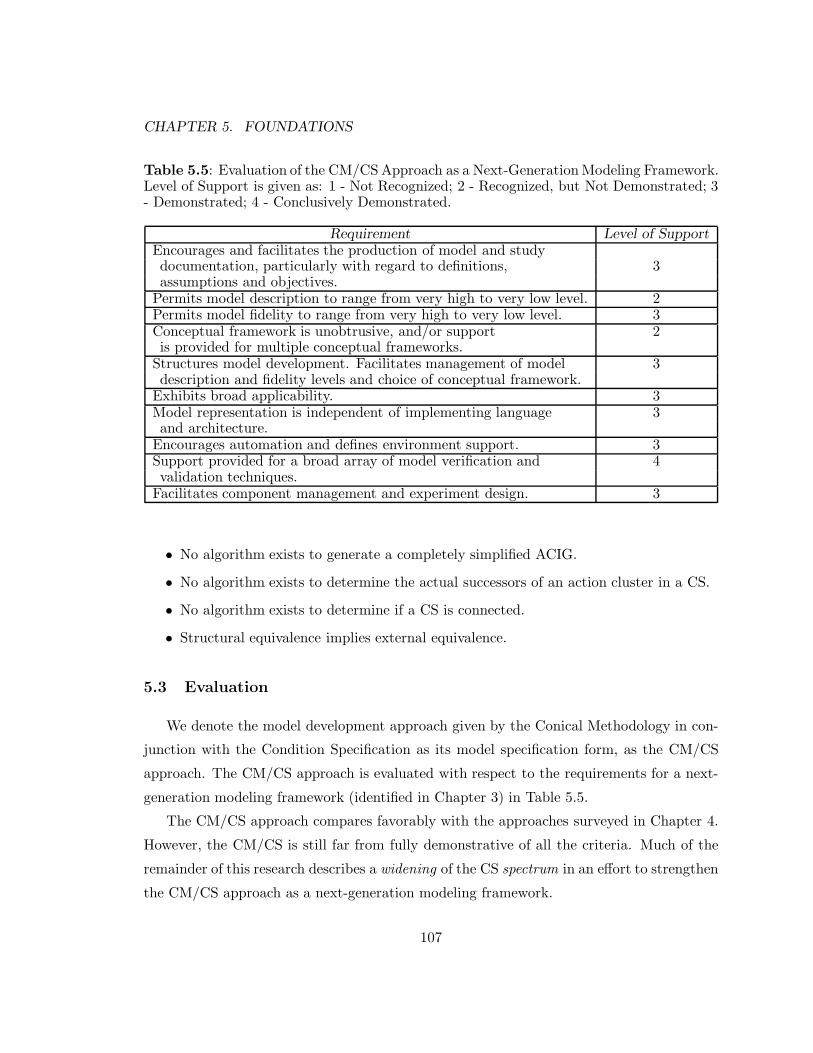
CHAPTER 5. FOUNDATIONS
Table 5.5: Evaluation of the CM/CS Approach as a Next-Generation Modeling Framework.Level of Support is given as: 1 - Not Recognized; 2 - Recognized, but Not Demonstrated; 3- Demonstrated; 4 - Conclusively Demonstrated.
Requirement Level of SupportEncourages and facilitates the production of model and studydocumentation, particularly with regard to definitions, 3assumptions and objectives.
Permits model description to range from very high to very low level. 2Permits model fidelity to range from very high to very low level. 3Conceptual framework is unobtrusive, and/or support 2is provided for multiple conceptual frameworks.
Structures model development. Facilitates management of model 3description and fidelity levels and choice of conceptual framework.
Exhibits broad applicability. 3Model representation is independent of implementing language 3and architecture.
Encourages automation and defines environment support. 3Support provided for a broad array of model verification and 4validation techniques.
Facilitates component management and experiment design. 3
• No algorithm exists to generate a completely simplified ACIG.
• No algorithm exists to determine the actual successors of an action cluster in a CS.
• No algorithm exists to determine if a CS is connected.
• Structural equivalence implies external equivalence.
5.3 Evaluation
We denote the model development approach given by the Conical Methodology in con-
junction with the Condition Specification as its model specification form, as the CM/CS
approach. The CM/CS approach is evaluated with respect to the requirements for a next-
generation modeling framework (identified in Chapter 3) in Table 5.5.
The CM/CS approach compares favorably with the approaches surveyed in Chapter 4.
However, the CM/CS is still far from fully demonstrative of all the criteria. Much of the
remainder of this research describes a widening of the CS spectrum in an effort to strengthen
the CM/CS approach as a next-generation modeling framework.
107

Chapter 6
MODEL REPRESENTATION
In the interest of clearness, it appeared to me inevitable that Ishould repeat myself frequently, without paying the slightestattention to the elegance of the presentation.
Albert Einstein, Relativity
In Chapter 3, a philosophy of simulation model development is described and a model
development abstraction consistent with this philosophy is proposed. The abstraction stip-
ulates a hierarchy of representations managed by a single, coherent, underlying method-
ology. The argument is made that this abstraction may enable the realization of a next-
generation modeling framework where emerging technologies and system-level requirements
can be cost-effectively incorporated into the simulation life cycle. In this chapter, and those
that succeed it, the feasibility of this argument is demonstrated utilizing Nance’s Conical
Methodology. The approach taken regarding model representation within the hierarchy is
neither top-down nor bottom-up. Investigation regarding the nature of the highest-level
form(s) has persisted within the context of the SMDE research effort since its inception,
and continues to occupy a prominent position (see [66]). The facilities and capabilities of
general purpose languages (GPLs) and simulation programming languages (SPLs) are also
well-studied. The approach taken here may best be described as inside-out. Overstreet’s
Condition Specification is assessed as most suited to occupy a mid-level position within
the hierarchy indicated by the framework – specifically as a form for model analysis. Its
relationship to both the envisaged higher-level and lower-level forms is addressed in Chap-
ters 6 through 9. By undertaking this investigation in an inside-out manner, the goal is
to facilitate a proper recognition of, and reconciliation between, the requirements of the
108

CHAPTER 6. MODEL REPRESENTATION
highest-level forms (as dictated primarily by the theories of modeling methodology) and
those of the lowest-level forms (as dictated primarily by system-level constraints).
6.1 Preface: Evaluating the Condition Specification
Overstreet never intends the CS as a modeler-level language. The program-like syntax
demands at least some buffering mechanism between the CS and a modeler. Similarly, the
statistical and reporting capabilities of the CS are not completely defined; nor are mecha-
nisms for list processing and time-flow described. These facilities, required for model imple-
mentation, are correctly viewed as too low-level for a specification language. Accordingly,
the CS is most suited to a mid-level position in the transformational hierarchy, primarily
serving as a target form for automated model diagnosis. This being established, several
issues must be addressed.
1. If a narrow-spectrum approach is adopted, a mid-level representation must exhibitcongruence with both the higher-level and lower-level representations. What can beestablished regarding the CS in this area?
2. Can the CS be adapted to provide wide-spectrum support?
3. What is the nature of the highest-level (modeler generated) representation(s)?
4. What is the nature of the underlying target implementations?
5. Can the CS be adapted – in either a narrow-spectrum or wide-spectrum approach –without sacrificing the analysis provided by the language?
In the following sections, the CS is evaluated through its application to a set of examples.
The language evaluation is such that the conclusions are applicable in the context of either a
narrow-spectrum or wide-spectrum approach, although the primary focus of the remainder
of this research is on widening the spectrum of the CS. The narrative is structured as a tuto-
rial, explicating the model development process under the Conical Methodology without an
explicit description of the highest-level representation form(s). For each example, observa-
tions are made regarding both model definition and model specification. This enables some
evaluation and discussion of the Conical Methodology, in addition to that involving the CS.
This seems appropriate given the observation from Chapter 4 that the relationship between
methodology and representation is a symbiotic one. Relevant adaptations and suggestions
regarding the CS accompany the examples.
109

CHAPTER 6. MODEL REPRESENTATION
0.8
0.2
0.4
0.6
LAN 9600
MODEM 2400
MODEM 1200
MODEM 300
PRTJESS
CPU1
CPU2
MVS COMPUTER SYSTEM
V
C
S
M
M
Figure 6.1: MVS System.
Table 6.1: MVS Interarrival Times.
Type of User Interarrival Times MeanModem 300 User Exponential 3200 SecondsModem 1200 User Exponential 640 SecondsModem 2400 User Exponential 1600 SecondsLAN 9600 User Exponential 266.67 Seconds
6.2 Example: Multiple Virtual Storage Model
Balci [19] presents an example involving a multiple virtual storage (MVS) batch com-
puter system. The MVS operates with two central processing units (CPUs). Users submit
batch programs to the MVS by using the submit command on an interactive virtual memory
(VM) computer system running under the CMS operating system. As shown in Figure 6.1,
the users of MVS via VM/CMS are classified into four categories: (1) users dialed in by
using a modem with 300 baud rate, (2) users dialed in by using a modem with 1200 baud
rate, (3) users dialed in by using a modem with 2400 baud rate, and (4) users connected to
the local area network (LAN) with 9600 baud rate. Each user develops the batch program
on the VM/CMS computer system and submits it to the MVS for processing. Based on
collected data, assume that the interarrival times of batch programs to the MVS with re-
spect to each user type are determined to have an exponential probability distribution with
corresponding means as shown in Table 6.1.
A batch program submitted first goes to the job entry subsystem (JES) of MVS. The
110

CHAPTER 6. MODEL REPRESENTATION
Table 6.2: MVS Processing Times.
Facility Processing Times MeanJESS Exponential 112 SecondsCPU1 Exponential 226.67 SecondsCPU2 Exponential 300 SecondsPRT Exponential 160 Seconds
JES scheduler (JESS) assigns the program to processor 1 (CPU1) with a probability of 0.6
or to processor 2 (CPU2) with a probability of 0.4. At the completion of program execution
on a CPU, the output of the program is sent to the user’s virtual reader on the VM/CMS
with a probability of 0.2 or to the printer (PRT) with a probability of 0.8. Assume that
all queues in the MVS system are first-come-first-served and each facility processes one
program at a time. The probability distribution of the processing times for programs by
each facility is given in Table 6.2.
Assuming that the simulation model reaches steady state after 3,000 programs, simulate
the system for 15,000 programs in steady state and construct confidence intervals for the
following performance measures (known values given in parentheses):
1. Utilization of the JESS (ρJESS = 0.70).
2. Utilization of CPU1 (ρCPU1 = 0.85).
3. Utilization of CPU2 (ρCPU2 = 0.75).
4. Utilization of the PRT (ρPRT = 0.80).
5. Average time spent by a batch program in the MVS computer system (W = 2400seconds).
6. Average number of batch programs in the MVS computer system (L = 15).
6.2.1 MVS model definition
The model definition for the MVS under the CM is given in Table 6.3. A discussion
of the derivation of the model is warranted. In defining the model, we attempt to portray
a modeler whose expertise is in the application domain and not in any particular area of
modeling or analysis or computer science (more about this later). The idea is to describe
the system in a “natural” way, i.e. in a way that is as close as possible to the model of the
111

CHAPTER 6. MODEL REPRESENTATION
Table 6.3: CM Object Definition for MVS Model.
Object Attribute Type RangeMVS system time temporal transitional indicative nonneg real
num served status transitional indicative 0..18000max served permanent indicative 18000
User type permanent indicative (m300,m1200,m2400,l9600)arrival temporal transitional indicative nonneg realarrival mean permanent indicative (266.67,640,1600,3200)
Job enter time permanent indicative nonneg realJess end service temporal transitional indicative nonneg real
status status transitional indicative (busy,idle)service mean permanent indicative 112cpu1 prob permanent indicative 0.6
Cpu1 end service temporal transitional indicative nonneg realstatus status transitional indicative (busy,idle)service mean permanent indicative 226.67prt prob permanent indicative 0.8
Cpu2 end service temporal transitional indicative nonneg realstatus status transitional indicative (busy,idle)service mean permanent indicative 300prt prob permanent indicative 0.8
Prt end service temporal transitional indicative nonneg realstatus status transitional indicative (busy,idle)
Set Type Member Type DescriptionJessQ d-set Job objects provide FIFO queue capabilitiesCpu1Q d-set Job objects provide FIFO queue capabilitiesCpu2Q d-set Job objects provide FIFO queue capabilitiesPrtQ d-set Job objects provide FIFO queue capabilities
112

CHAPTER 6. MODEL REPRESENTATION
system that tends to naturally exist in the mind of the modeler. Where useful for clarity,
the convention is adopted to set object names in typewriter font and attribute names in
italics.
6.2.1.1 Objects
The first object is mandated by the methodology: the top-level object. We give it a
name, MVS and associate the model indexing attribute with it. Attributes for number served
and maximum number served are also defined.
Next, four user objects are described – one for each of the possible sources of jobs.
This can be effected two ways in the methodology: by defining four separate objects, e.g.
m300User, m1200User, etc., or by defining a single object, User, which has attributes
indicating its type, arrival mean and time of next arrival. In this manner, the instantiation,
as handled by the specification language, must assign the correct attribute values. These
two approaches yield externally equivalent models (see Chapter 5). The latter approach is
adopted here.
Since the user object is viewed as creating jobs which enter the system,1 an object Job is
defined and given an attribute enter time (to represent the time in which the job entered the
system). Realizing that a job, once created, will be sent to the JESS, the need is recognized
for an object representing the JESS.
The object Jess is defined to have attributes representing its service mean and the time
at which the next end-of-service occurs. Also defined are an attribute indicating its status
and an attribute giving the probability with which a job leaving the JESS will travel to
CPU1. This leads naturally to the definition of the object Cpu1 and subsequently Cpu2
and then Prt. However, at this point a recognition may be made that jobs routed to these
“facilities” may need to be stored (in first-come-first-served order) for processing.
We elect to make use of the CM provisions for sets to represent the queues for each of
the facilities. The sets are typed as d-sets, since set membership must be determined during
execution. The members are identified as being job objects. The CM doesn’t describe set
1Note, the derivation of the user and job objects to some extent hinges upon the modeler’s perceptionof model dynamics. Specifically, the user is envisioned as creating jobs, according to a particular rate,that are sent to the JESS. This illustrates that model definition and model specification are not completelyindependent processes, even though they produce artifacts that may be considered independent.
113

CHAPTER 6. MODEL REPRESENTATION
implementation, i.e. no “default” attributes or operations are defined. The set is described
as providing “FIFO queue capabilities.” At this point in the model definition process, it
may be sufficient to assume the attributes and operations are available to determine queue
size, provide insertion and deletion, and so on.
An interesting observation is that the CM, unlike some simulation programming lan-
guages, e.g. SIMSCRIPT, doesn’t provide “ownership” among objects. That is, in a SIM-
SCRIPT description, the Cpu object might be declared as owning a queue (or FIFO set).
Access would be provided in a manner such as:
remove first Job from queue(Cpu)
as long as the context provides the identification of the Cpu. Under the CM (assuming use
of the CS) the CPUs and queues, in a manner similar to the previously described definition
of the user object, could be defined and specified three ways:
1. As independent objects, Cpu1, Cpu2, Cpu1Q, Cpu2Q.
2. As a single object with an a priori determined number of “instances,” e.g. Cpu[1..2],CpuQ[1..2].
3. As a single object with an undetermined number of possible “instances.”
Methods (1) and (2) provide a convenient means by which to exploit the relationship be-
tween a cpu and its queue. Method (3) provides the requisite information, but the access
mechanism may be somewhat clumsy. In this case, each object requires an attribute (e.g.
id) to uniquely identify it within the set. And the condition that gives the begin service for
a cpu must be expressed in terms such as:
not empty(CpuQ) and (Cpu.status = idle) and (Cpu.id = CpuQ.id)
Suitable, perhaps, to express behavior at a low level, but higher-level representations must
permit more elegant descriptions.
6.2.1.2 Activity sequences
Since the definition provided by the CM is object-based it might lead naturally, for a
given modeler, to an object-based (process) visualization of model behavior. In this context,
the model is viewed very broadly as follows.
114

CHAPTER 6. MODEL REPRESENTATION
1. Schedule the “arrival” of the next job.
2. Wait for arrival time.
3. Create Job and record enter time.
4. Place Job in JessQ.
5. Return to 1.
Figure 6.2: Activity Sequence for User.
1. Whenever the JessQ is not empty and status of Jess is idle:
2. Remove first Job in JessQ.
3. Set status to busy.
4. Wait for end-of-service.
5. Determine route for Job.6. If route is to Cpu1, put Job in Cpu1Q.
7. Else put job in Cpu2Q.
8. Set status to idle.
9. Return to 1.
Figure 6.3: Activity Sequence for Jess.
Four user objects are instantiated (one for each type: m300, m1200, m2400 and l9600).
The appropriate arrival mean is assigned, and the user proceeds according to the activity
sequence given in Figure 6.2. The behaviors of the JESS, the CPUs and the printer are
given in Figures 6.3, 6.4 and 6.5 respectively.
Notice that, in this model, the job is depicted as having no “active” lifetime. Another,
equally valid, model of this system could describe the job as an active object. Such an
approach might define the lifetime of a job as given in Figure 6.6. Either definition may
conform to a given modeler’s “natural” view of the underlying system. The key methodolog-
ical issue is the permission of either description in an unconstrained fashion. The Conical
Methodology provides this.
115

CHAPTER 6. MODEL REPRESENTATION
1. Whenever the Cpu queue is not empty and status of Cpu is idle:
2. Remove first Job in Cpu queue.
3. Set status to busy.4. Wait for end-of-service.
5. Determine route for job.
6. If route is to Prt, put job in PrtQ.
7. Else calculate total time in system for job.
8. Set status to idle.9. Return to 1.
Figure 6.4: Activity Sequence for Cpu.
1. Whenever the PrtQ is not empty and status of Prt is idle:
2. Remove first Job in PrtQ.
3. Set status to busy.
4. Wait for end-of-service.5. Calculate total time in system for Job.
6. Delete Job.
7. Set status to idle.
8. Return to 1.
Figure 6.5: Activity Sequence for Printer.
116

CHAPTER 6. MODEL REPRESENTATION
1. Enter system.
2. Wait for Jess.3. Use Jess.
4. Determine route from Jess.
5. If route is to Cpu1:
6. Wait until Cpu1 is available.
7. Use Cpu1.
8. Determine route from Cpu1.9. Else:
10. Wait until Cpu2 is available.
11. Use Cpu2.
12. Determine route from Cpu2.
13. If route is to Prt:14. Wait until Prt is available.
15 Use Prt.
16. Record total time in system.
17. Exit system.
Figure 6.6: Alternate Approach: Activity Sequence for Job.
117

CHAPTER 6. MODEL REPRESENTATION
6.2.1.3 Flexibility in model representation
Of course, in the MVS model the need for all the objects defined in Table 6.3 is ques-
tionable. In fact, someone knowledgeable in queueing theory, or an SPL such as GPSS,
could construct a program for this system with fewer objects and very few lines of code.
This program would doubtless be totally comprehensible to the modeler, and could in all
likelihood be explained to a decision maker, who may be a novice to many of these concepts.
However, the model is constructed in this fashion to make an important point:
An evolving tenet of modeling methodology is that as systems being modeled growmore and more complex, the need will become ever greater to allow people withthe domain knowledge to create the models.
The reasoning behind this position is as follows. The current paradigm requires that a do-
main expert “communicate,” often in an unstructured and ad hoc fashion, with a modeling
expert, or expert tool user. For complex systems this leads to many levels of uncertainty.
The modeler is never quite sure that he understands the domain and likewise the domain
expert seldom has 100 percent faith in the produced model. This approach requires the
extensive use of prototype models, which are successively refined in an attempt to remove
these “gray areas.” However, this may not always be the most cost-effective means of pro-
ducing a model. The modeling effort typically does not cease with the first “production”
form. Many models represent a large investment, and therefore have lengthy lifetimes, dur-
ing which the model evolves considerably. Keeping a modeling consultant on contract for
this potentially lengthy period is a costly proposition. Also, the potential exists that the
original modeler may no longer be available subsequent to the original development; thus
model maintenance means re-communicating the domain knowledge to a new modeler.
Hence, a belief is evolving that the methodology and environment should permit the
domain expert to describe the model and, to as great an extent as possible, do so in his or
her own terms. This seems the best way to foster the development of a correct model – a
critical factor to the provision of decision support (see Chapter 3).
In summary, the modeling methodology must be flexible. It should provide the guidelines
and constraints that foster time-proven techniques that encompass good modeling practice.
But the flexibility must remain with the modeler to allow the description of novel systems.
The CM achieves this very well.
118

CHAPTER 6. MODEL REPRESENTATION
6.2.1.4 Support for statistics gathering
The description of behavior given in the model lifetimes does not include the computa-
tions required to gather statistics, nor are all the necessary attributes defined to accomplish
it. The question is, should they be? Consider these facts:
1. The CM stipulates that the objectives (in terms of the performance measures) beexplicitly stated.
2. Existing SPLs like GPSS and SIMSCRIPT provide a great deal of statistical infor-mation “automatically,” without requiring anything on the part of the programmer,except to ask for the information collected.
If the objectives are stated in terms of CM-defined objects and attributes then the statistical
calculations, since these are mathematically well-defined, need not be required from the
modeler when describing a model or its behavior.2
These issues primarily impact the representational forms. Note, however, that if this
approach is adopted for the MVS model, the attribute enter time for the object Job would
not need to be defined. Simply stating the objective of calculating the mean time in the
system for jobs would be sufficient. This leads to the production of an object seemingly
having no attributes. Can the object be deleted? The methodology indicates yes, since an
object is only defined in terms of its attributes (and their values). But, the object does in
fact have attributes. The attributes are those required to facilitate statistics gathering and
reporting, based on the stated model objectives, and one of these attributes must represent
the time at which the object entered the system. These attributes could, in fact, be seen in
some augmented object definition.
As illustrated previously with its handling of sets, the CM does not advocate any partic-
ular implementation of concepts. As long as the “things” being described have a well-defined
meaning (and this can perhaps only be determined in the context of the representational
forms and supporting environment), the CM should, and does, permit flexibility. Descrip-
tions of model behavior should be permitted without stipulating, for instance, the imple-
mentation of set mechanisms. Similarly, it should be permissible to define an object and
2For analytical purposes, a representation that explicitly captures these definitions and computationsmay be desirable. But this can be automatically generated from the underlying model specification and theproperly formulated description of model objectives.
119

CHAPTER 6. MODEL REPRESENTATION
not define explicitly any attributes for it – if the only interest in the object is a set of statis-
tical observations regarding its behavior and no other attributes are needed to realize the
behavior. The realization of statistical behavior could perhaps be determined by examining
an augmented object definition and specification. If the object has no attributes in the
augmented definition, then the object has no function in the model. Therefore, we adopt
the view that the situation described above is acceptable, especially in light of the alterna-
tive: forcing the modeler to explicitly define and specify statistics gathering for every model
developed. Since these things can be automated, in accordance with the automation-based
paradigm that influences the CM, they should be automated.
6.2.2 MVS model specification
In this section, the Condition Specification is examined with regard to the MVS model
defined in the previous section. The MVS transition specification resulting from this devel-
opment is given in Appendix D.
6.2.2.1 Specification of sets in the CS
Through its provisions for set definition, the Conical Methodology provides a convenient
means by which to utilize a common mechanism in simulation: the queue. A queue may
be viewed as a set with some ordering properties that dictate the set insertion and deletion
operations. The Condition Specification does not explicitly support the concept of sets.
Sets used within the CM definition, however, can be described using the extant CS syntax.
However, the encumbrance to the description is significant. An object that may belong to
an ordered set (or queue), as in the case of the job object from the MVS example, must
be given attributes that describe both its location and the time it entered that location.
Selection of the first object in the queue could be accomplished by quantification over all
existing jobs with a given location, e.g. “in waiting queue for Jess,” and selecting the one
with the smallest enter time. Since the CS is not envisioned as a modeler-level language,
this places no undue inconvenience on the modeler in terms of the description of model
behavior. The CS representations are envisaged as being automatically generated from
higher forms. However, a couple of observations can be made at this point:1. A high-level representation will likely provide convenient mechanism for appealing to
sets (and queues).
120

CHAPTER 6. MODEL REPRESENTATION
Table 6.4: Set Operations for the Extended Condition Specification. Operations may bequalified with well-formed expressions of model attributes as well as keywords such as first,
last, all, and unique.
Name Call Returns DescriptionInsert insert(object, set <, qualifier >) – Insert object into set.Remove remove(set <, qualifier >) Object Remove object from
set.Empty empty(set) Boolean True if set has no
members.Member member(object, set) Boolean True if object in set.Find find(set, qualifier) Set, Object Find object or subset
based on qualifier.
2. As noted previously, interesting model-based questions exist that cannot be answeredautomatically. For these instances, the CS may need to be viewed by an analyst.
These observations beg the question, should the concept of sets, and operations on sets,
as provided by the CM, be added to the CS? If so, can sets be added without hampering
the analytic capabilities of the CS? Another interesting question involves the specification
of sets versus their implementation: can a model translator determine efficient mechanisms
for implementing sets according to their usage? For example, a queue may be used at
the highest levels of description when a counter or other simple variable is sufficient at
the execution level. A modeler may choose to represent a set of failed machines (in the
machine interference problem described subsequently) and choose a machine for repair by
finding the first failed from that set. This could be implemented by two attributes status
and time-of-failure, and avoid the overhead associated with an actual implementation of a
set. Capabilities such as these must be defined to permit truly implementation-independent
model development, but these types of problems are essentially the same as those that have
confronted optimized compilation for years.
The general capabilities for defining and using sets are recommended for the Condition
Specification. The syntax for the set operations, insert, remove, empty, member and
find is given in Table 6.4.3
3Note that specialized queue operations, e.g. enqueue and dequeue, could be defined based on thegeneral operations insert and remove.
121

CHAPTER 6. MODEL REPRESENTATION
6.2.2.2 Object typing
A modeling approach may permit typing of objects. SIMSCRIPT provides a mechanism
through which entities may be classified as permanent or temporary. In GPSS, objects are
viewed as dynamic (transactions) or static (facilities). In the parlance of the CS, designating
an object as temporary or permanent could be used to indicate whether or not a destroy
operation is permissible on the object. Designating an object as dynamic or static could
provide an indication of its proper use with regard to model sets, i.e. an enqueue operation
should perhaps be illegal on a static object.
However, since the CM stipulates that attributes, not objects, are typed, no mechanism
for object typing is described for the CS.
6.2.2.3 Parameterization of alarms
Overstreet provides the facility to parameterize alarms. Alarm parameterization would
seem unnecessary and unadvised for the following reason: use of parameters permits the
separation of the object from the alarm by using a single alarm for many objects. For ex-
ample, when alarm(failure,i). This seems bad conceptually, and in a software engineering
sense, increases the coupling of the specification. A better specification for this would be,
for some i:1..N:: when alarm(machine[i].failure).
In the former case, the use of alarm parameters may indicate a poorly designed model.
Model analysis should perhaps be defined to detect this type of situation. However, alarm
parameters are useful not only to identify the object to which the alarm belongs, but also
in a general sense to allow an expression in terms of model attributes to be evaluated when
the alarm is set, and then used when the alarm goes off. To disallow this facility may
cause a modeler to resort to the creation of extra, artificial, attributes, to store values
for this same purpose. For this reason, the parameterization of alarms remains a part of
the representation provided in the Condition Specification. Nontheless, how this facility
manifests itself in the higher-level representational forms is unclear.
6.2.2.4 On the relationship of action clusters and events
Consider the situation described in Figure 6.7. The illustration represents, essentially, an
“event” description of an end-of-service at the JESS. Certainly, a high-level representation
122

CHAPTER 6. MODEL REPRESENTATION
Whenever Jess.end service
Jess.status := idle
Job := REMOVE(JessQ)
if (random() < Jess.cpu1 prob)
INSERT(Job,Cpu1Q)else
INSERT(Job,Cpu2Q)
Figure 6.7: Event Description for JESS End-of-Service.
would permit the model to be described in similar terms. The question is: how is this
represented in the CS, where each action must be under the domain of a single, explicitly
defined condition? One possible solution is illustrated in Figure 6.8. In this case, the event
is decomposed into the three action clusters pictured. The condition for the first AC is
the condition on the occurrence of the event. The two remaining conditions represent the
conjunction of the event condition with a condition relating to the value of the random
variate.4 This process requires the creation of two Boolean variables. Within the CM, these
may be defined as attributes of the top-level model object. However, the model, as defined
by the modeler, will not have these attributes defined – since the specification mechanism
will be at a much higher level than the CS. We observe,
these are attributes needed to implement the higher-level representation usingthe CS syntax.
This type of phenomenon may commonly occur throughout the hierarchy. Management of
these additional attributes is an issue of concern for a modeling methodology and environ-
ment supporting model evolution through transformations. However, the interest of this
research effort, with respect to the CS, is primarily at the action cluster level; the man-
agement problem for these variables isn’t addressed further. However, this type of problem
has been addressed within the development of compiler theory. Appeal to these results is
4As shown in Chapter 8, this type of augmentation is required only when each AC must be consideredindependently. The knowledge that the event (when alarm) condition must always be accompanied by oneof the two remaining ACs, as can be depicted in the ACIG, permits the simplification of the AC conditionsand obviates the need for “dummy” variables.
123

CHAPTER 6. MODEL REPRESENTATION
WHEN ALARM(Jess.end service):
Boolean1 := true
Boolean2 := random() < Jess.cpu1 prob
Boolean1 AND Boolean2:Jess.status := idle
Job := REMOVE(JessQ)
INSERT(Job,Cpu1Q)
Boolean1 := false
Boolean1 AND NOT Boolean2:
Jess.status := idle
Job := REMOVE(JessQ)
INSERT(Job,Cpu2Q)
Boolean1 := false
Figure 6.8: Action Clusters Corresponding to Event Description for JESS End-of-Service.
made to resolve any variable management issues not detailed specifically herein. For the
context of this effort, the convention for naming these attributes follows the form, B$1, B$2,
etc. These are considered attributes of the top-level object, but are not listed in the object
definition.
6.2.2.5 The report specification
Overstreet does not prescribe a specific form for the report specification, but instead
indicates how the interface between the report specification and the transition specification
might be formed using a program designed to compute statistics (see Figure 5.4). An
alternative form for the report specification is proposed. The specification is comprised of
statements taking the form:
report expression as “title”
The expression may be given in terms of model objects and attributes and common, well-
defined statistical measurements (so that the calculations needed to gather statistics can
be automatically generated from the information provided in the object definitions and
124

CHAPTER 6. MODEL REPRESENTATION
REPORT TIME IN STATE Jess.status = busy OVER STEADY STATE DURATION AS “Utilization of Jess”
REPORT TIME IN STATE Cpu1.status = busy OVER STEADY STATE DURATION AS “Utilization of Cpu1”
REPORT TIME IN STATE Cpu2.status = busy OVER STEADY STATE DURATION AS “Utilization of Cpu2”
REPORT TIME IN STATE Prt.status = busy OVER STEADY STATE DURATION AS “Utilization of Prt”
REPORT MEAN TIME IN SYSTEM FOR OBJECT Job AS “Average time of job in system”REPORT TIME WEIGHTED MEAN NUMBER IN SYSTEM FOR OBJECT Job AS “Average number of jobs in system”
Figure 6.9: MVS Report Specification.
transition specification). The report specification for the MVS model is given in Figure 6.9.
6.2.2.6 On automating statistics gathering
When seeking to automatically generate the attributes and actions necessary to ac-
complish the statistics gathering specified by the report specification, the problem may be
addressed in two ways:
1. Generate the necessary attributes and actions to collect and calculate the statisticalinformation as the simulation is running.
2. Generate the necessary actions to write the appropriate value changes to “logs” whichcan be post-processed to gather the requisite statistical information.
The first approach is adopted by many extant SPLs. The second method is often utilized in
distributed and parallel discrete event simulation to prevent the statistical gathering rou-
tines from becoming either a source of nondeterminism or a performance bottleneck. The
appropriateness of either approach depends upon the characteristics of the target imple-
mentation as well as the language in which the executable model is represented.
Clearly, both approaches are automatable. The later approach is the simplest, requiring
only that a set of output actions be added as appropriate within a transition specification,
and that a post-processor be provided to generate the statistical values from the logs. The
feasibility of the former approach merits further discussion. We consider the approach in
terms of augmenting an existing object and transition specification.
125

CHAPTER 6. MODEL REPRESENTATION
Augmented object specification. To produce an augmented object specification that
facilitates “on-the-fly” statistics gathering, some mechanism must automatically generate
attributes to accomplish the tasks specified by the report specification. This augment-
ing mechanism requires some well-defined naming scheme to provide general assurance
against creating any compilation problems by having conflicts arise between the “baseline”
(modeler-generated) and augmented attribute naming. As before, the details of this ap-
proach are beyond the scope of this work, but for purposes of this example we use the
following scheme.5 For a report specification containing,
report time in state object.attrib = value over steady state duration as “...”
we define the following attributes:
• timeInState$attribValue for the object. This attribute contains the accumulated sim-ulation time in steady state (if defined) for which the attribute has the correspondingvalue.
• timeInState$attribValueStart for the object. This attribute contains the simulationtime at which the object last assumed the value.
For a report specification containing,
report mean time in system for object object as “...”
we define the following attributes:
• enterTime$system (or enterTime$setname) for the object. This attribute contains theentry time for the object instance into the system (or set).
• timeInSys$object for the system object (or timeInSetname for a set). This attributecontains the accumulated time in steady state (if defined) for all the instances of thegiven class of object in the system (or set). (The time is given by the differencebetween object creation and destruction – for the system, or by insert and removeoperations – for a set.)
For a report specification containing,
report time weighted mean number in system for object object as “...”
we define the following attributes:
5Assume that the dollar symbol ($) is not permitted in modeler-level attribute naming. Attributescontaining the $ are recognized as being system generated.
126

CHAPTER 6. MODEL REPRESENTATION
t3
1
2
3
4
5
t2t1 t4 t5 t6
Simulation time
Number inSystem
Figure 6.10: Calculating a Time-Weighted Average for Number in System. Averagenumber in system is given by the total area divided by the duration time of the simulation.
• numInSys$object for the system object (or numInSetname for a set). This attributecontains the current number of object instances of the given class inside the system(or set).
• numInSysTime$object for the system object (or numInSetnameTime for a set). Thisattribute contains the simulation time at which the number of object instances of thegiven class inside the system (or set) was last set.
• numInSysArea$object for the system object (or numInSetnameArea for a set). Thisattribute contains the accumulated area in steady state (if defined) of object instancesof the given class inside the system (or set). This concept is illustrated in Figure 6.10.
The following are candidate system-generated attributes (belonging to the system object –
a $ symbol could be added for consistency):
• systemTime. Contains the current value of simulation time.
• steadyState. A Boolean indicating whether or not steady state has been reached fora given model execution.
• steadyStateStartTime. Contains the value of simulation time when system steadystate was achieved.
A comprehensive set of statistical reporting attributes (and computations) has not been
defined here. A wide variety of statistical functionality can be automatically supported
127

CHAPTER 6. MODEL REPRESENTATION
similar to that provided by most simulation programming languages. This presentation
is simply intended to give the flavor of how attribute monitoring in an augmented object
specification may be defined.
Augmented transition specification. In order to provide monitoring of “baseline” at-
tributes, the system must generate a description of the assignments to augmented attributes
that accompany any change in value of a monitored baseline attribute. For example, given
a report specification containing,
report time in state obj.attrib = value over steady state duration as “...”
we define the following calculations:
Baseline Action Augmented Actionsobj.attrib := value obj.attrib := value
obj.timeInState$attribValueStart := systemTimeobj.attrib := value′ if ((obj.attrib = value) and (steadyState))
obj.timeInState$attribValue := obj.timeInState$attribValue +(systemTime - obj.timeInState$attribValueStart)
obj.attrib := value′
For a report specification containing,
report mean time in system for object obj as “...”
we define the following calculations:
Baseline Action Augmented Actionscreate(obj) create(obj)
obj.enterTime$system := systemTimedestroy(obj) if (steadyState)
sysobj.timeInSys$obj := sysobj.timeInSys$obj +(systemTime - obj.enterTime$system)
destroy(obj)
For a report specification containing,
report time weighted mean number in system for object obj as “...”
we define the following calculations:
128

CHAPTER 6. MODEL REPRESENTATION
Baseline Action Augmented Actionscreate(obj) create(obj)
if (steadyState)sysobj.numInSysArea$obj := sysobj.numInSysArea$obj +sysobj.numInSys$obj * (systemTime - sysobj.numInSysTime$obj)
sysobj.numInSys$obj := sysobj.numInSys$obj + 1sysobj.numInSysTime$obj := systemTime
destroy(obj) if (steadyState)sysobj.numInSysArea$obj := sysobj.numInSysArea$obj +sysobj.numInSys$obj * (systemTime - sysobj.numInSysTime$obj)
sysobj.numInSys$obj := sysobj.numInSys$obj - 1sysobj.numInSysTime$obj := systemTimedestroy(obj)
Can augmented calculations be added as ACs? The most direct approach to aug-
menting a CS would be to adopt a stratified approach in which any additional calculations
generated to facilitate statistics gathering are incorporated within the existing CAP/AC
paradigm underlying the CS. But, whenever a monitored attribute is referenced in the
baseline specification, the attendant statistical calculations need to be atomic with the
reference. Consider the following fragment from the MVS example,
Jess Begin Service Jess.status = idle and not empty(JessQ):
Jess.status := busyset alarm(Jess.end service, exp(Jess.service mean))
Jess End Service Route Cpu1 B$1 and B$2:
Jess.status := idleJob := remove(JessQ)insert(Job,Cpu1Q)B$1 := false
At end service the total busy time is accumulated, using the calculation:
jess.timeInState$statusBusy := jess.timeInState$statusBusy +(systemTime - jess.timeInState$statusBusyStart)
If this action is incorporated into a state-based successor of the end service AC, the possi-
bility for race conditions will have been introduced between the new statistical AC – which
reads the value of jess.timeInState$statusBusyStart, and the begin service AC – which sets
the value of jess.timeInState$statusBusyStart. In order to prevent race conditions, the
129

CHAPTER 6. MODEL REPRESENTATION
condition for begin service might have to be conjoined with a condition indicating the com-
pletion of the new statistical AC. This approach could quickly become unattractive. An
alternative approach would be to relax the CAP/AC paradigm in the augmented specifi-
cation, permitting the conditions on statistics gathering to appear as sub-conditions in an
AC. In light of these two alternatives, the method of statistics gathering through logs seems
superior in this context.
6.2.2.7 The experiment specification
To facilitate the experimentation process, the following information must typically be
provided by a modeler:
1. Condition for start of model’s steady state.
2. Random number seeds.
3. Number of replications to perform.
4. Name(s) of input/output files.
Many other details may also be provided. For example, the choice of architecture may be
specified (or perhaps a best choice can be provided by the model analyzer – given some
global objective like “find most efficient implementation”).
To the extent that the information involved in model experimentation can be utilized
for analysis, it may be desirable to capture it at the CS level. We propose an experiment
specification for the CS, but do not prescribe its form.
6.3 Example: Traffic Intersection
A simulation model of the traffic intersection (TI) at Prices Fork Road and West Campus
Drive in Blacksburg, Virginia may adopt the structure illustrated in Figure 6.11. A single
traffic light with north, south, east and west directions controls vehicular movement within
each of the nine lanes of the intersection. The intersection itself is conceptually divided
into twenty-five blocks through which vehicles travel; while the location of a vehicle moving
through the actual intersection is a continuous function, the blocks provide a convenient
means of approximating a traffic flow pattern (with reasonable fidelity) within a discrete
event simulation of the system.
130

CHAPTER 6. MODEL REPRESENTATION
9
8
321
67
D.R
KROF
ES
CIRP
WEST CAMPUS DR.
AB
C
D E F G H
L M N O P
Q R S T UV W
X Y
I J K
E
S
W
N
Figure 6.11: The Intersection of Prices Fork Road and West Campus Drive.
131

CHAPTER 6. MODEL REPRESENTATION
Table 6.5: Traffic Intersection Interarrival Times.
Lane Interarrival Distribution Mean1 Exponential 20.61 Seconds2 Unknown 8.52 Seconds3 Unknown 6.21 Seconds6 Unknown 8.53 Seconds7 Unknown 5.52 Seconds8 Unknown 3.77 Seconds9 Unknown 5.63 Seconds
The objective of the simulation is to provide a light timing sequence which improves the
throughput for the intersection. The following definitions are used to describe the model,
1. N = number of lanes in the intersection.
2. m = number of vehicles departing from lane j : j = 1, 2, . . . , N
3. Arrival Time = the time at which a vehicle joins the end of the waiting line or thetime at which the front end of the vehicle moves across the first white line in the lane(if no waiting line exists).
4. Departure Time = the time at which the rear end of the vehicle clears the last whiteline in the travel path.
5. IATij = interarrival time of the ith (i = 1, 2, . . . , m) vehicle in lane j : j = 1, 2, . . . , N .
6. Vehicle Waiting Time = departure time - arrival time
7. Wij = waiting time of the ith vehicle in lane j (i = 1, 2, . . . , m; j = 1, 2, . . . , N).
8. WTj = waiting time of all vehicles in lane j : j = 1, 2, . . . , N = 1m
∑mi=1 Wij
9. E(Wj) = expected waiting time of vehicles in lane j : j = 1, 2, . . . , N = 1m
∑mi=1 Wij =
1mWTj
Vehicle interarrival times and travel times are presented in Tables 6.5 and 6.6.6 During
the observation period, traffic flow in the north-south, north-east, and north-west directions
was negligible. Therefore the model contains no information about traffic from lanes 4 and
5. Also, the effects of pedestrian traffic (as provided by a pedestrian light control) within the
intersection are not present in the model. According to the observed system, the probability
6The values presented are based on observations of the system taken during “rush hour” conditions inMay 1987 by the CS 4150 simulation class at Virginia Tech.
132

CHAPTER 6. MODEL REPRESENTATION
Table 6.6: Traffic Intersection Travel Times.
Lane Travel Time Distribution Mean1 Uniform 4.87 Seconds2 Uniform 2.70 Seconds3 Uniform 1.85 Seconds6 Uniform 2.67 Seconds7 Uniform 4.30 Seconds
7(r) Uniform 2.43 Seconds8 Uniform 4.32 Seconds
9(l) Uniform 4.75 Seconds9(r) Uniform 1.84 Seconds
of a right turn by a vehicle traveling in lane 7 is 0.524 and the probability of a right turn
from lane 9 is 0.494. The model allows right turn on red for these lanes.
The light timing sequence is illustrated in Figure 6.12. The light follows a cycle of 40
seconds of green for south-north traffic (while other directions in red), followed by 3 seconds
where all directions are under red (for intersection clearance), followed by a 62 second green
period for east-west traffic. During this 62 second span, south-north lanes are under red for
the entire time, while west-east lanes get a green after 22 seconds.
6.3.1 TI model definition
The CM model definition for the TI is prefaced with some remarks regarding system
behavior.
6.3.1.1 Vehicular behavior
Traffic through the intersection is governed by the following assumptions. A vehicle
arrives at the intersection and waits until it reaches the head of the line. In general, if the
light is green and the block immediately ahead in the path of the vehicle is available, the
vehicle moves into that block and travels a time proportional to the total travel time for
a vehicle in the given lane. Provisions are made to ensure that the first vehicle entering
the intersection on a new green waits until the intersection has cleared before proceeding.
Subsequent vehicles entering the intersection during the same green do not check this clear-
ance. Only vehicles making specified right turns may proceed under red, i.e. all vehicles in
133

CHAPTER 6. MODEL REPRESENTATION
40 3
40 3 62
Direction: West to East
Direction: East to West
Direction: South to North
40 3 62
RedLegend: Green
22 40
Figure 6.12: Light Timing Sequence Diagram.
the model follow the established rules of the road.
Figure 6.13 illustrates the movement of a vehicle in lane 1. A vehicle traveling through
the intersection in lane 1 does so by moving through blocks X,U,M,L, and C in that order.
The first vehicle entering the intersection through lane 1 after a new east-west green must
wait for the intersection to clear from the previous green (which was for the south-north
traffic in lanes 8 and 9). This means determining that blocks I, J, K, L, M, N, T, and U
are clear. Note that the clearance of blocks Q, R and S should not be part of this criterion
since these are the blocks involved in a right turn from lane 9 which is permitted under
south-north red. The blocks Q, R and S can safely be ignored by the clearance check for
lane 1 due to the 3 second delay in which all lanes are under red following the south-north
green.7
Each vehicle traveling through lane 1, however, must check clearance for blocks A, B,
7This is true since the travel time for vehicles going south-to-west in lane 9 through blocks Q, R and Sis 2.23 seconds. Further, if the intersection is full when the south-north green ends, traffic backup cannotcause the delay to exceed the 2.23 seconds to clear blocks Q,R and S for the last vehicle through.
134
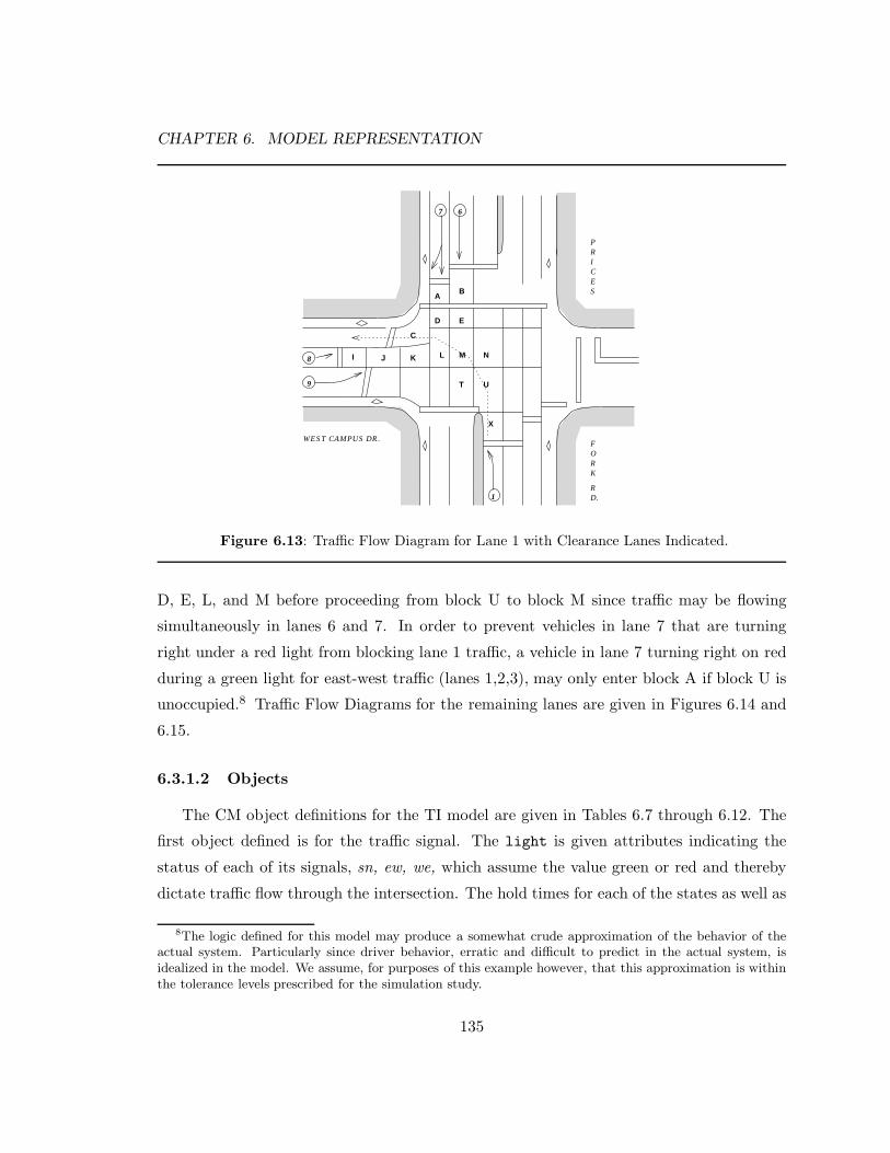
CHAPTER 6. MODEL REPRESENTATION
9
8
1
67
D.R
KROF
ES
CIRP
WEST CAMPUS DR.
AB
C
D E
L M N
T U
X
I J K
Figure 6.13: Traffic Flow Diagram for Lane 1 with Clearance Lanes Indicated.
D, E, L, and M before proceeding from block U to block M since traffic may be flowing
simultaneously in lanes 6 and 7. In order to prevent vehicles in lane 7 that are turning
right under a red light from blocking lane 1 traffic, a vehicle in lane 7 turning right on red
during a green light for east-west traffic (lanes 1,2,3), may only enter block A if block U is
unoccupied.8 Traffic Flow Diagrams for the remaining lanes are given in Figures 6.14 and
6.15.
6.3.1.2 Objects
The CM object definitions for the TI model are given in Tables 6.7 through 6.12. The
first object defined is for the traffic signal. The light is given attributes indicating the
status of each of its signals, sn, ew, we, which assume the value green or red and thereby
dictate traffic flow through the intersection. The hold times for each of the states as well as
8The logic defined for this model may produce a somewhat crude approximation of the behavior of theactual system. Particularly since driver behavior, erratic and difficult to predict in the actual system, isidealized in the model. We assume, for purposes of this example however, that this approximation is withinthe tolerance levels prescribed for the simulation study.
135

CHAPTER 6. MODEL REPRESENTATION
9
8
2 D.R
KROF
ES
CIRP
WEST CAMPUS DR.
G
L M N O
T UV
Y
I J K
9
8
3 D.R
KROF
ES
CIRP
WEST CAMPUS DR.
H
O P
T UW
7
D.R
KROF
ES
CIRP
WEST CAMPUS DR.
A
D
L
S
6
D.R
KROF
ES
CIRP
WEST CAMPUS DR.
B
E
M
T
Lane Diagram for Lane 2 Lane Diagram for Lane 3
Lane Diagram for Lane 6 Lane Diagram for Lane 7S
Figure 6.14: Traffic Flow Diagrams for Lanes 2, 3, 6 and 7S with Clearance Lanes Indicated.
136

CHAPTER 6. MODEL REPRESENTATION
7
D.R
KROF
ES
CIRP
WEST CAMPUS DR.
A
C
D
8
21
67
D.R
KROF
ES
CIRP
WEST CAMPUS DR.
B
E
L M N O
UV
X Y
I J K
9
D.R
KROF
ES
CIRP
WEST CAMPUS DR.
Q R S9
321
67
D.R
KROF
ES
CIRP
WEST CAMPUS DR.
B
E H
L M O P
Q R S T UV W
X Y
Lane Diagram for Lane 7R Lane Diagram for Lane 8
Lane Diagram for Lane 9L Lane Diagram for Lane 9R
G
Figure 6.15: Traffic Flow Diagrams for Lanes 7R, 8, 9L and 9R with Clearance Lanes Indicated.
137

CHAPTER 6. MODEL REPRESENTATION
Table 6.7: CM Object Definition for Top-Level Object and Traffic Signal
Object Attribute Type Rangeti numCars status transitional indicative nonneg int
maxCars permanent indicative 18600light sn status transitional indicative (green,red)
ew status transitional indicative (green,red)we status transitional indicative (green,red)snGreen temporal transitional indicative nonneg realsnRed temporal transitional indicative nonneg realewGreen temporal transitional indicative nonneg realweGreen temporal transitional indicative nonneg realsnGreenTime permanent indicative 40.00 secondssnClearTime permanent indicative 3.00 secondsewGreenTime permanent indicative 22.00 secondsweGreenTime permanent indicative 40.00 seconds
Table 6.8: CM Object Definition for Lanes
Object Attribute Type Rangelane[1..9] arrival temporal transitional indicative nonneg real
arrival mean permanent indicative positive realprobTurn permanent indicative positive realnewGreen status transitional indicative (true,false)
the time at which the next state change will occur are also provided as attributes for the
light.
An object for each lane is defined as shown in Table 6.8. Within the CM, when the
number of object instances is a priori determinable, an object may be defined using “array
notation” to indicate that number. In this case, light[1..9] is used for notational conve-
nience. Of course, since lanes 4 and 5 are not represented in the model, the definition could
be, lane[i: i=1,2,3,6,7,8,9]. The details of the definitional syntax are not elements
of the methodology crucial within the scope of this effort. Of primary concern is that the
“meaning” of a given definition or specification be unambiguously conveyed.
We represent the topology of the intersection by creating an object, block for each of the
twenty-five blocks pictured in Figure 6.11. Each block has an attribute, status, indicating
by busy or idle, whether or not the block is occupied by a vehicle.
138

CHAPTER 6. MODEL REPRESENTATION
Table 6.9: CM Object Definition for Blocks.
Object Attribute Type Rangeblock[A..Y] status status transitional indicative (busy,idle)
Table 6.10: CM Object Definition for Lane Waiting Lines.
Set Type Member Type DescriptionlaneQ[1..9] d-set LanexCar objects provide FIFO queue capabilities
Since cars arrive at the intersection and potentially are made to join a waiting line
prior to actually entering the intersection proper, we appeal to the CM provisions for set
definition (as in the previous example) to provide a queue for each lane.
Finally, objects representing vehicular traffic are defined. We define one object “class”
for each of the paths through the intersection, i.e. an object for vehicles in lane 1, one for
vehicles in lane 2, one for vehicles in lane 7 turning right, etc. Each object has attributes
that dictate its path through the intersection proper and holding times for each of the blocks
in the path.
6.3.2 TI model specification
Since, in the actual system, the vehicles provide the activity of interest, a natural means
of describing model dynamics is to depict the lifetimes of vehicles traveling in the various
lanes. These lifetimes are depicted in the activity sequences of Figures 6.16 through 6.24.
The “implementations” of these lifetimes in the CS are given in the transition specification
for the TI model in Appendix E. The report specification is presented in Figure 6.25.
6.3.2.1 Using functions in the Condition Specification
Overstreet identifies a function specification in which a modeler may describe functions.
These functions may be invoked within the transition specification to aid in the description
of model behavior. Overstreet places no restrictions on the use of functions. Given the per-
ceived need to provide flexibility to a modeler, this stance is appropriate. However, since
functions are exempt from the analysis defined by the CS, perhaps their use should be lim-
139

CHAPTER 6. MODEL REPRESENTATION
Table 6.11: CM Object Definition for Vehicles (Part I).
Object Attribute Type Rangelane1Car getBlockU temporal transitional indicative nonneg real
getBlockM temporal transitional indicative nonneg realgetBlockL temporal transitional indicative nonneg realgetBlockC temporal transitional indicative nonneg realexit temporal transitional indicative nonneg realblockXTime permanent indicative 1.12 secondsblockUTime permanent indicative 1.02 secondsblockMTime permanent indicative 0.87 secondsblockLTime permanent indicative 0.61 secondsblockCTime permanent indicative 1.25 seconds
lane2Car getBlockV temporal transitional indicative nonneg realgetBlockO temporal transitional indicative nonneg realgetBlockG temporal transitional indicative nonneg realexit temporal transitional indicative nonneg realblockYTime permanent indicative 0.68 secondsblockVTime permanent indicative 0.68 secondsblockOTime permanent indicative 0.67 secondsblockGTime permanent indicative 0.67 seconds
lane3Car getBlockP temporal transitional indicative nonneg realgetBlockH temporal transitional indicative nonneg realexit temporal transitional indicative nonneg realblockWTime permanent indicative 0.63 secondsblockPTime permanent indicative 0.62 secondsblockHTime permanent indicative 0.60 seconds
lane6Car getBlockE temporal transitional indicative nonneg realgetBlockM temporal transitional indicative nonneg realgetBlockT temporal transitional indicative nonneg realexit temporal transitional indicative nonneg realblockBTime permanent indicative 0.73 secondsblockETime permanent indicative 0.69 secondsblockMTime permanent indicative 0.64 secondsblockTTime permanent indicative 0.61 seconds
lane7SCar getBlockD temporal transitional indicative nonneg realgetBlockL temporal transitional indicative nonneg realgetBlockS temporal transitional indicative nonneg realexit temporal transitional indicative nonneg realblockATime permanent indicative 0.52 secondsblockDTime permanent indicative 0.84 secondsblockLTime permanent indicative 0.80 secondsblockSTime permanent indicative 0.78 seconds
140

CHAPTER 6. MODEL REPRESENTATION
Table 6.12: CM Object Definition for Vehicles (Part II).
Object Attribute Type Rangelane7RCar getBlockD temporal transitional indicative nonneg real
getBlockC temporal transitional indicative nonneg realexit temporal transitional indicative nonneg realblockATime permanent indicative 0.46 secondsblockDTime permanent indicative 0.91 secondsblockCTime permanent indicative 1.06 seconds
lane8Car getBlockJ temporal transitional indicative nonneg realgetBlockK temporal transitional indicative nonneg realgetBlockL temporal transitional indicative nonneg realgetBlockM temporal transitional indicative nonneg realgetBlockN temporal transitional indicative nonneg realgetBlockG temporal transitional indicative nonneg realexit temporal transitional indicative nonneg realblockITime permanent indicative 0.45 secondsblockJTime permanent indicative 0.86 secondsblockKTime permanent indicative 0.82 secondsblockLTime permanent indicative 0.40 secondsblockMTime permanent indicative 0.39 secondsblockNTime permanent indicative 0.72 secondsblockGTime permanent indicative 0.68 seconds
lane9LCar getBlockR temporal transitional indicative nonneg realgetBlockS temporal transitional indicative nonneg realgetBlockT temporal transitional indicative nonneg realgetBlockU temporal transitional indicative nonneg realgetBlockO temporal transitional indicative nonneg realgetBlockH temporal transitional indicative nonneg realexit temporal transitional indicative nonneg realblockQTime permanent indicative 0.94 secondsblockRTime permanent indicative 0.86 secondsblockSTime permanent indicative 0.43 secondsblockTTime permanent indicative 0.42 secondsblockUTime permanent indicative 0.58 secondsblockOTime permanent indicative 0.76 secondsblockHTime permanent indicative 0.76 seconds
lane9RCar getBlockR temporal transitional indicative nonneg realgetBlockS temporal transitional indicative nonneg realexit temporal transitional indicative nonneg realblockQTime permanent indicative 0.73 secondsblockRTime permanent indicative 0.74 secondsblockSTime permanent indicative 0.37 seconds
141
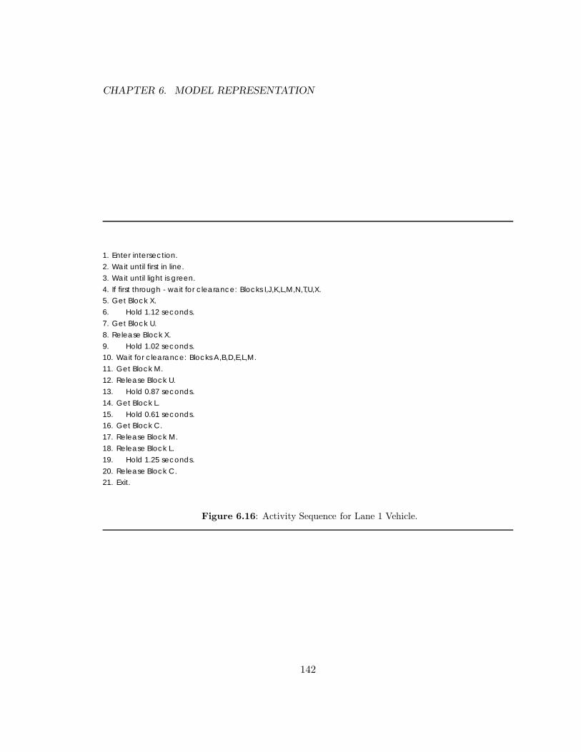
CHAPTER 6. MODEL REPRESENTATION
1. Enter intersection.
2. Wait until first in line.
3. Wait until light is green.
4. If first through - wait for clearance: Blocks I,J,K,L,M,N,T,U,X.5. Get Block X.
6. Hold 1.12 seconds.
7. Get Block U.
8. Release Block X.
9. Hold 1.02 seconds.10. Wait for clearance: Blocks A,B,D,E,L,M.
11. Get Block M.
12. Release Block U.
13. Hold 0.87 seconds.
14. Get Block L.
15. Hold 0.61 seconds.16. Get Block C.
17. Release Block M.
18. Release Block L.
19. Hold 1.25 seconds.
20. Release Block C.21. Exit.
Figure 6.16: Activity Sequence for Lane 1 Vehicle.
142

CHAPTER 6. MODEL REPRESENTATION
1. Enter intersection.
2. Wait until first in line.
3. Wait until light is green.
4. If first through - wait for clearance: Blocks I,J,K,L,M,N,T,U,Y.5. Get Block Y.
6. Hold 0.68 seconds.
7. Get Block V.
8. Release Block Y.
9. Hold 0.68 seconds.10. Get Block O.
11. Release Block V.
12. Hold 0.67 seconds.
13. Get Block G.
14. Release Block O.15. Hold 0.67 seconds.
16. Release Block G.
17. Exit.
Figure 6.17: Activity Sequence for Lane 2 Vehicle.
1. Enter intersection.
2. Wait until first in line.
3. Wait until light is green.4. If first through - wait for clearance: Blocks O,T,U,W.
5. Get Block W.
6. Hold 0.63 seconds.
7. Get Block P.
8. Release Block W.9. Hold 0.62 seconds.
10. Get Block H.
11. Release Block P.
12. Hold 0.60 seconds.
13. Release Block H.14. Exit.
Figure 6.18: Activity Sequence for Lane 3 Vehicle.
143

CHAPTER 6. MODEL REPRESENTATION
1. Enter intersection.2. Wait until first in line.
3. Wait until light is green.
4. Get Block B.
5. Hold 0.73 seconds.
6. Get Block E.
7. Release Block B.8. Hold 0.69 seconds.
9. Get Block M.
10. Release Block E.
11. Hold 0.64 seconds.
12. Get Block T.13. Release Block M.
14. Hold 0.61 seconds.
15. Release Block T.
16. Exit.
Figure 6.19: Activity Sequence for Lane 6 Vehicle.
1. Enter intersection.
2. Wait until first in line.3. Wait until light is green.
4. Get Block A.
5. Hold 0.52 seconds.
6. Get Block D.
7. Release Block A.8. Hold 0.84 seconds.
9. Get Block L.
10. Release Block D.
11. Hold 0.80 seconds.
12. Get Block S.13. Release Block L.
14. Hold 0.78 seconds.
15. Release Block S.
16. Exit.
Figure 6.20: Activity Sequence for East-Bound Lane 7 Vehicle.
144

CHAPTER 6. MODEL REPRESENTATION
1. Enter intersection.
2. Wait until first in line.
3. If light is red and east-west is green- wait for clearance: Blocks L,M.
4. Get Block A.
5. Hold 0.46 seconds.6. Get Block D.
7. Release Block A.
8. Hold 0.91 seconds.
9. Get Block C.
10. Release Block D.11. Hold 1.06 seconds.
12. Release Block C.
13. Exit.
Figure 6.21: Activity Sequence for South-Bound Lane 7 Vehicle.
ited to non-model-specific activity, such as the generation of random numbers and random
variates? Regardless, functions should have no unanalyzable effects on model attributes. In
the absence of the highest-level representations, however, further guidance on the use of
functions in the CS is impracticable.
6.3.2.2 Another set operation
Developing the transition specification for the TI model identifies the need for another
set operation. Here, the need arises since d-sets are defined (the lane queues) which may
have different “classes” of objects as members. For example, the set laneQ[9] may have
lane9RCar objects and lane9LCar objects. Model behavior varys according to which class
of object is removed. Specifically, a car turning right in lane 9 enters the intersection and
holds block Q for 0.73 seconds, whereas a car turning left holds block Q for 0.94 seconds.
Furthermore, the left-turning car must establish a different set of clearances than the right
turning car. We define the set operator, class, which interrogates an object within a set
and returns the value of its class, i.e. the object name that appears in the CM definition.
The operator must be passed the set name and a pointer to the object. A typical use of
145

CHAPTER 6. MODEL REPRESENTATION
1. Enter intersection.2. Wait until first in line.
3. Wait until light is green.
4. If first through - wait for clearance: Blocks B,E,I,L,M,X,U,Y,V,O.
5. Get Block I.
6. Hold 0.45 seconds.7. Get Block J.
8. Release Block I.
9. Hold 0.86 seconds.
10. Get Block K.
11. Release Block J.
12. Hold 0.82 seconds.13. Get Block L.
14. Hold 0.40 seconds.
15. Get Block M.
16. Release Block K.
17. Hold 0.39 seconds.18. Get Block N.
19. Release Block L.
20. Release Block M.
21. Hold 0.72 seconds.
22. Get Block G.
23. Release Block N.24. Hold 0.68 seconds.
25. Release Block G.
26. Exit.
Figure 6.22: Activity Sequence for Lane 8 Vehicle.
146

CHAPTER 6. MODEL REPRESENTATION
1. Enter intersection.2. Wait until first in line.
3. Wait until light is green.
4. If first through - wait for clearance: Blocks B,E,L,M,X,U,Y,V,O,W,P,H.
5. Get Block Q.
6. Hold 0.94 seconds.7. Get Block R.
8. Release Block Q.
9. Hold 0.86 seconds.
10. Get Block S.
11 Hold 0.43 seconds.
12. Get Block T.13. Release Block R.
14. Hold 0.42 seconds.
15. Get Block U.
16. Release Block S.
17. Release Block T.18. Hold 0.58 seconds.
19. Get Block O.
20. Release Block U.
21. Hold 0.76 seconds.
22. Get Block H.
23. Release Block O.24. Hold 0.76 seconds.
25. Release Block H.
26. Exit.
Figure 6.23: Activity Sequence for West-Bound Lane 9 Vehicle.
147

CHAPTER 6. MODEL REPRESENTATION
1. Enter intersection.
2. Wait until first in line.4. If light is red - wait for clearance: Blocks D,L,S,Q.
5. Get Block Q.
6. Hold 0.73 seconds.
7. Get Block R.
8. Release Block Q.9. Hold 0.74 seconds.
10. Get Block S.
11 Hold 0.37 seconds.
12. Release Block R.
13. Release Block S.14. Exit.
Figure 6.24: Activity Sequence for East-Bound Lane 9 Vehicle.
REPORT MEAN TIME IN SYSTEM FOR OBJECT Lane1Car AS “Average travel time of vehicles in Lane 1”REPORT MEAN TIME IN SYSTEM FOR OBJECT Lane2Car AS “Average travel time of vehicles in Lane 2”
REPORT MEAN TIME IN SYSTEM FOR OBJECT Lane3Car AS “Average travel time of vehicles in Lane 3”
REPORT MEAN TIME IN SYSTEM FOR OBJECT Lane6Car AS “Average travel time of vehicles in Lane 6”
REPORT MEAN TIME IN SYSTEM FOR OBJECT Lane7SCar AS “Average travel time of east-bound vehicles in Lane 7”
REPORT MEAN TIME IN SYSTEM FOR OBJECT Lane7RCar AS “Average travel time of south-bound vehicles in Lane 7”REPORT MEAN TIME IN SYSTEM FOR OBJECT Lane8Car AS “Average travel time of vehicles in Lane 8”
REPORT MEAN TIME IN SYSTEM FOR OBJECT Lane9LCar AS “Average travel time of west-bound vehicles in Lane 9”
REPORT MEAN TIME IN SYSTEM FOR OBJECT Lane9RCar AS “Average travel time of east-bound vehicles in Lane 9”
Figure 6.25: TI Report Specification.
148

CHAPTER 6. MODEL REPRESENTATION
this operation may be a Boolean test of the form:
class(laneQ[9],first) = Lane9LCar
where the modifier first indicates the object at the head of an ordered set.
6.3.3 Object-based versus object-oriented
This section concludes with some thoughts regarding the CM as an object-based approach
to model development as contrasted with object-oriented approaches.
For purposes of this discussion, the following are considered characteristic of the object-
oriented paradigm (OOP):9
1. Association of objects in a system to objects in a model.
2. Class descriptions.
3. Inheritance structure.
4. Object behavior encapsulated within methods.
5. Object instantiation.
6. Object “communication” through message passing.
A long-running debate in Computer Science raises the question, is object-oriented a superior
approach? Certainly, the OOP has advantages over traditional programming languages from
a general software engineering perspective. Still, overuse of features like multiple inheritance
can lead to code that is nearly impossible to comprehend. Our question has a slightly
different focus: from the point of view of discrete event simulation model development,
is OOP superior to the object-based perspective of the CM? We assert that the answer
to this question is emphatically no. First of all, the CM provides (1), (2), (3) and (5)
from the list above. The CM has no notion of “method” and places no restrictions on the
manner in which objects read and write the values of attributes. These issues fall within
the domain of the model representation form(s). Certainly an SMSDL could encapsulate
model dynamics in such a manner, and enforce “communication” through a message passing
9Many may argue that other features such as polymorphism and operator overloading are also integralto the OOP. We consider these traits to be more an aspect of object-oriented programming languages thanthe OOP itself.
149

CHAPTER 6. MODEL REPRESENTATION
structure, but at what cost? As argued in the previous section, an important characteristic
of any methodology for simulation model development is providing flexibility to the modeler
– specifically, not forcing a single restrictive conceptual framework on every problem. The
constraints of the object-oriented paradigm can cause a modeler to define a system in a
very unnatural way. Take, for instance, the TI model presented in this section. An OOP
characterization would allow the blocks of the intersection proper to be defined as objects
(just as done with the CM), but a vehicle object is forced to send a message to a block
object to determine the status of the block. Communication among model objects, when it
occurs, should be expressible (at the highest, modeler-end, level) in a natural manner. One
may view a pilot and a co-pilot in an aviation simulation as communicating through passed
messages, but describing driver behavior as passing messages to – and receiving them from
– asphalt, is another matter altogether.
6.4 Example: Colliding Pucks
The Colliding Pucks problem, hereafter referred to as pucks, is based on the pool ball
systems described by Goldberg [89]. In the basic pucks model, rigid disks move along a flat
surface and collide with surface boundaries and other disks. The kinematics of the pucks
system are detailed below.
6.4.1 Kinematics of pucks
A pucks system can be viewed as illustrated in Figure 6.26. A large variety of models
are possible for pucks based on the myriad physical assumptions that can be made about
the system. For this example, the following system characteristics are assumed:
1. The surface is a rectangular table aligned with the x-y origin.
2. The table is frictionless.
3. Table boundaries have infinite mass.
4. All pucks are of equal mass.
5. Collisions are elastic and total system energy is conserved.
150

CHAPTER 6. MODEL REPRESENTATION
y
x
Figure 6.26: Colliding Pucks System.
Each puck has a position (x, y), velocity vector V = (νx, νy), and radius, r. The table
boundaries are defined by the equations:
x = 0, x = n, y = 0, y = m (6.1)
Two types of collisions occur in the system: (1) puck-boundary collisions, and (2) interpuck
collisions. For each type of collision a simulation must provide both collision prediction (or
detection) and collision resolution.
6.4.1.1 Pucks and boundaries: collision prediction
At any given point in simulation time, we can calculate the time until the next boundary
collision for any puck in the system. This calculation is a function of the puck’s position
and velocity, and is a prediction, not a guarantee.10 Times to boundary collisions are given
10Subsequent to the calculation of the boundary collision time and prior to the collision itself, the puckmay be involved in an interpuck collision, potentially causing the predicted boundary collision time to beincorrect.
151

CHAPTER 6. MODEL REPRESENTATION
by:
tx =
tright ≡ n−(x+r)νx
if νx > 0
tleft ≡ x−r−νx
if νx < 0
∞ if νx = 0
(6.2)
ty =
ttop ≡ m−(y+r)νy
if νy > 0
tbottom ≡ y−r−νy
if νy < 0
∞ if νy = 0
(6.3)
For any puck, the time until the most imminent predicted boundary collision is:
tcollision = min(tx, ty) (6.4)
6.4.1.2 Pucks and boundaries: collision resolution
To resolve a puck-boundary collision we update the puck’s position and velocity. If
the position and velocity of the puck are given by (x, y) and (νx, νy) respectively, and
tcollision = τ , then the position of the puck (at the time of the collision) is:
x′ = x + νxτ (6.5)
y′ = y + νyτ (6.6)
And the new velocity is:
V =
(−νx,−νy) if tx = ty
(−νx, νy) if tx < ty
(νx,−νy) if ty < tx
(6.7)
6.4.1.3 Pucks and pucks: collision prediction
To determine the time until a collision between any two pucks, we solve the quadratic
equation that results from the interpretation of the distance squared between the centers
of the two pucks as a function of time. Given two pucks A and B with positions, velocities,
and radii (xA, yA), (νxA, νyA
), rA and (xB, yB), (νxB, νyB
), rB respectively then the distance
squared between pucks is given by:
d2 = (xB − xA)2 + (yB − yA)2 (6.8)
152

CHAPTER 6. MODEL REPRESENTATION
To determine when the AB collision occurs (if one occurs), we evaluate the equation:
d2(t) = (rA + rB)2 (6.9)
To solve for t in Equation 6.9 we let d2(t) = at2 + bt+ c− (rA + rB)2. The coefficients are
given by:
a = (νxB− νxA
)2 + (νyB− νyA
)2 (6.10)
b = 2[(xB − xA)(νxB− νxA
) + (yB − yA)(νyB− νyA
)] (6.11)
c = (xB − xA)2 + (yB − yA)2 − (rA + rB)2 (6.12)
Solve for t by evaluating:
t =−b±
√b2 − 4ac
2a(6.13)
If the quadratic equation yields two positive real roots, then the collision time, tcollision, is
taken as the minimum of the two roots from Equation (6.13) (the larger value represents
the time at which the trailing edges of the pucks will be touching i.e. the pucks will have
passed through one another). Two negative real roots or a negative discriminant indicate
that the pucks are moving away from one another or the pucks are on parallel courses and
no future collision is possible. When two pucks are traveling in the same direction and at
the same speed then a (Equation (6.10)) is zero.11
6.4.1.4 Pucks and pucks: collision resolution
Resolving interpuck collisions requires: (1) updating the puck positions to those at the
time of the collision, and (2) updating the puck velocities.
Puck positions are updated as in the puck-boundary case by Equations (6.5) and (6.6).
Updating the velocities involves: (1) establishing the normal and tangential component
velocities of the collision (and thereby creating a t-n coordinate system), (2) updating the
puck velocities relative to the t-n system, and (3) translating these updated velocities back
into the x-y coordinate system. Figure 6.27 illustrates a collision between two pucks and
shows their component velocities.
11An implementation of the system must check for this to avoid division by zero errors.
153

CHAPTER 6. MODEL REPRESENTATION
6
-
y
50
100
150
50 100 150 200 250
x
&%'$q &%'$qA B
tangential component
normal component
Figure 6.27: Component Velocities of an Interpuck Collision.
We establish the normal component as a vector between the positions of the two pucks:
N = (xn, yn)
xn = xB−xA√(xB−xA)2+(yB−yA)2
yn = yB−yA√(xB−xA)2+(yB−yA)2
(6.14)
The tangential component is perpendicular to the normal and can be established by rotating
the normal vector ninety degrees:
T = (−yn, xn) (6.15)
To update the velocities of the two pucks, relative to the t-n system, we swap the velocities
in the normal component and leave the velocities in the tangential component unchanged.
V ′A = (VB · N ,VA · T ) (6.16)
V ′B = (VA · N ,VB · T ) (6.17)
With the new velocities calculated in the t-n system, we must translate the velocities back
into x-y coordinates. Let Ux and Uy be the unit vectors of x and y respectively. And let Rx
and Ry be vectors defined as:
Rx = (Ux · N ,Ux · T ) (6.18)
Ry = (Uy · N ,Uy · T ) (6.19)
154

CHAPTER 6. MODEL REPRESENTATION
5
8 9 10 11
&%'$q&%'$q&%'$q@@@
1 2
3
-
@@I
Figure 6.28: A Collision Among Three Pucks.
Then the velocities of the pucks A and B in the x-y coordinate system are given by:
V ′′A = (V ′
A · Rx,V ′A · Ry) (6.20)
V ′′B = (V ′
B · Rx,V ′B · Ry) (6.21)
6.4.1.5 Collisions involving multiple pucks
The collision resolution scheme described above generates updated velocities for two
pucks involved in a collision. When several pucks collide simultaneously, the algorithm
must pairwise resolve the collisions.12 In some cases, the resultant velocities of an N-disk
collision are not strictly independent of the serial order of resolution using this scheme.
One such case is presented in Figure 6.28. In the Figure, Puck 1 is at (8,5) and V1 is
(1,0); Puck 2 is stationary at position (10,5); and Puck 3 is at (10 +√
2, 5 −√
2) with
V3 = (−1, 1). Thus we see that Puck 1 is striking Puck 2 head on while at the same time
Puck 3 collides with Puck 2 at an angle of forty-five degrees. We have two choices for pairwise
collision resolution: resolve collision (1,2) then collision (2,3) or resolve collision (2,3) then
collision (1,2). Table 6.13 shows the velocity changes, and the differing resultant trajectories
12Since no general closed form solution exists for the N-body problem of colliding disks, the mathematicsdescribed is only partially correct. We assume that these approximations are acceptable within the tolerancelevels prescribed for the simulation study.
155

CHAPTER 6. MODEL REPRESENTATION
Table 6.13: Order of Resolution Dependence in Multiple Puck Collisions.CASE I CASE II
Initially Coll(1,2) Coll(2,3) Initially Coll(2,3) Coll(1,2)
V1 (1,0) (0,0) (0,0) (1,0) (1,0) (-1,0)V2 (0,0) (1,0) (−1
2 ,32) (0,0) (-1,1) (1,1)
V3 (-1,1) (-1,1) (12 ,−
12) (-1,1) (0,0) (0,0)
for both cases.13
Using the pairwise collision resolution scheme we must assure that the system always
processes the same multiple puck collision in the same pairwise order – to provide repro-
ducibility of simulation results. We may achieve this by simply requiring that in any multiple
puck collision the collision involving the puck with the smallest identifier is processed first,
then the collision involving the remaining disk with the smallest identifier, and so on.14
6.4.2 A literature review of pucks solutions
The pucks model was developed specifically as a benchmark for parallel discrete event
simulation protocols [29, p. 56]. The nature of pucks – a system where the level of inherent
parallelism seems high, but for which few assumptions can be made regarding both the
times and frequencies of interactions among system objects – makes it interesting in this
respect. On the other hand, the model formulation clearly indicates a misperception of the
fundamental nature of discrete event simulation; a misperception that seems to permeate
much of PDES. For pucks, no modeling objectives are defined. The PDES view would seem
to be that if a program approximates reality in some sense, then that program must be,
by definition, a simulation. The development of Chapter 3 clearly contradicts this view.
A simulation is, first-and-foremost, a tool for decision support. Fundamental to decision
support is the formulation of a modeling objective. As stated in Chapter 2, only through
the modeling objective can meaning be assigned to a model or its results. This fact cannot
be overstated.
A brief review of pucks-related literature further illustrates this significant misappre-
13For Case I, a third collision will occur – between Puck 1 and Puck 2 – in which the final x-componentvelocities given in the Table are switched.
14This scheme is utilized in [29, 52, 89, 103, 138].
156

CHAPTER 6. MODEL REPRESENTATION
hension of the nature of discrete event simulation.
6.4.2.1 Goldberg’s model
In his thesis, Goldberg [89] originally defines the pucks system for an object-oriented
simulation of pool ball motion.
Time flow. Goldberg discusses the pool ball simulation as implemented using two time
flow mechanisms, fixed-time increment (FTI) and time of next event (TNE).15 He observes
a significant problem with an FTI implementation of the simulation is a tradeoff between
speed and accuracy, noting that accuracy of the simulation is compromised using FTI since a
collision cannot be simulated exactly at the time it occurs. At each time step the simulation
must determine if two balls have collided by determining if the balls overlap. The smaller
the time step, the greater the accuracy of the simulation; but larger time steps are viewed
as more desirable to reduce the amount of computation within the simulation. Goldberg
concludes that no good heuristics exist that indicate the optimum selection of time step
size [89, p. 6].
According to Goldberg, an event-based implementation does not suffer from the accuracy
problem of the FTI approach. In Goldberg’s TNE algorithm, all possible future collisions
are scheduled, i.e. each ball calculates the most imminent collision between itself and every
other ball and any cushions. When a ball undergoes a collision and updates its velocity, it
cancels all scheduled collisions and schedules new ones based on its new trajectory. Goldberg
claims that the TNE approach is computationally more efficient than the FTI approach in
typical cases (e.g. when the average number of collisions per time step is less than n/logn,
where n is the number of pool balls in the simulation). Algorithms for the object-oriented
solution are given in Appendix C. (Note: Figures C.1 and C.2 illustrate the behavior for
balls and cushions. The behaviors for corners and pockets are similar to cushion behavior
and are not illustrated.) The logic of the object-oriented implementation is similar to that
defined for the pure TNE implementation except that the event list is “distributed” as
objects schedule events via message passing (given the three message types: NewVelocity,
15Goldberg [89, p. 3] refers to these as the “two major temporal simulation methods: time step simulationand discrete event simulation.”
157

CHAPTER 6. MODEL REPRESENTATION
Collision, and Cancel).
Implications of an object-oriented solution. The object-oriented simulation execu-
tion paradigm utilized by Goldberg requires that for any value of simulation time an object
may execute (process outstanding messages) at most once (running an object more than
once for any value of simulation time can lead to incorrect results since the object may
behave differently than if allowed to process all messages at once). This causes difficulty in
modeling systems with zero time delay or, using Goldberg’s terminology, “instantaneous”
events. To illustrate this, consider the following scenario: Ball-1, resting against a cushion,
is being struck by another ball, Ball-2. Three things happen simultaneously: Ball-2 knocks
Ball-1 into the cushion, Ball-1 bounces off the cushion, Ball-1 collides with Ball-2 sending
Ball-2 back into the table. Suppose the simulation executive schedules the object execution
in the order: Ball-1, Ball-2, Cushion.16 Ball-1 receives a Collision message from Ball-2 and
sends a NewVelocity message to the Cushion then terminates. Ball-2 processes the Collision
message it sent to itself, sends a NewVelocity message to the Cushion and terminates. The
Cushion processes the NewVelocity messages. The NewVelocity message from Ball-1 causes
the Cushion to send a Collision message to Ball-1. But Ball-1 has already executed for this
value of simulation time. Further, we see that any ordering of object processing leads to a
similar conclusion. To circumvent this inherent problem of the scheduling policy Goldberg
allows the second collision to be processed after a small delay.
Sectored model. Since the complexity of the object-oriented pool ball model is domi-
nated by the number of messages, Goldberg proposes a sectorized model to cut down on the
number of messages required for the average case. In a sectored model, a ball determines
if it will collide only with the other balls in its sector, not all the balls on the table. How-
ever, the addition of sectors is not without its costs: new messages for entering and leaving
sectors are required as well as mechanisms for dealing with collisions on and around sector
boundaries. Goldberg’s algorithms for ball and sector behaviors are given in Appendix C.
The sectored algorithm contains five types of messages, which can be categorized into
two groups. First, the VelocityChange and NewVelocity messages convey information about
16During execution each object in turn is allowed to process all messages it has received whose timestampsare equal to the simulation time.
158

CHAPTER 6. MODEL REPRESENTATION
a ball’s change in velocity. Second, the Collision, SectorEntry and SectorDeparture messages
schedule future events, involving two balls or a ball and a sector, based on the ball’s new
velocity.17
In detail, the algorithm behaves as follows. When a ball changes velocity it sends a
VelocityChange message to each sector it occupies. Unless the ball is stationary, each
occupied sector schedules a SectorDepart for the ball. Involved sectors send NewVelocity
messages to all adjacent sectors and to all balls within the sectors themselves. If the ball’s
trajectory intercepts an adjacent sector’s perimeter, the sector schedules a sector entry by
sending a SectorEntry message to the ball and one to itself.
A NewVelocity message is received by each ball that shares a sector with the ball whose
velocity has changed. These balls determine whether they are to collide with the ball in
question. If a ball predicts a collision then it sends a Collision message to the ball whose
velocity has changed and one to itself.
Sector entry and departure. Goldberg identifies the perimeter of a sector by a list
of its corners (this representation permits myriad polygonal sector forms). The edges of a
sector connect adjacent corners in the list, e.g. a rectangular sector requires a list of five
corner points, since the first corner repeats at the end of the list. The sector departure time
of a ball from a sector is the instant a ball leaving the sector crosses its perimeter. Thus,
the departure time is the maximum of the times at which the ball crosses the sector’s edges
and corners. The sector entry time is the time an entering ball first crosses the perimeter.
Instantaneous messages. The problem of instantaneous messages, and the resolution
of allowing a small delta to separate velocity changes in serial collisions, further complicates
Goldberg’s sectored model by allowing balls to pass through each other. For example,
suppose Ball-1 is stationary against the edge of a sector and Ball-2 collides with Ball-1 as
it enters the sector. Because of a the delay in the NewVelocity message (from Ball-2 to
the sector to Ball-1 with artificial delay) Ball-1 will not recognize Ball-2 until they overlap.
Goldberg addresses this problem by having Ball-1 schedule an immediate collision with
Ball-2. This works in most cases, with some loss of accuracy in the solution. However, this
17Each of these messages is sent by the object scheduling the interaction to both itself and the otherinvolved object.
159

CHAPTER 6. MODEL REPRESENTATION
solution still allows one ball to pass through another, e.g. if the time it takes for Ball-2 to
pass through Ball-1 is less than the delay.
6.4.2.2 The JPL model
The implementation of Goldberg’s simulation, as a colliding rigid disks model, for the
Time Warp Operating System (TWOS) is described in [29, 103]. According to [29], the
pucks model embodies several “fundamental” problems of PDES. The authors describe
these as:
1. Modularization Strategy. Dividing the work of building software in an organized andrational way.
2. Object-Oriented Design. Object-oriented design of sequential simulations often stopswith the identification of the software objects corresponding to physical objects inthe simulated world or well-defined abstract objects. In distributed simulation, “thedesigner must also respond to performance concerns [29, p. 27].” Objects (realized asprocesses) must have an appropriate granularity and bottlenecks should be avoided.
3. Synchronization of Message Communication. The number of messages should notgrow too rapidly with the number of objects.
4. Dynamic Recomposition of Objects and Processes. A desirable quality is the abilityof objects to decompose and aggregate for performance enhancement.
5. Dynamic Load Management. Process/processor mappings must be amenable to dy-namic reconfiguration to admit maximal performance.
A pucks model is implemented using two mini-languages, Circles – for the kinematics
and dynamics of the system, and Twang – containing the object interaction protocols.
The sectored implementation uses a simpler message protocol than that of Goldberg.
Each sector examines the trajectories of all pucks within its boundaries and schedules only
the earliest predicted collision. The sector reawakens at the time of the collision, and then
causes the involved pucks to change velocity. This cycle is repeated until the condition for
termination is met.
This protocol has the advantage that no mechanism is needed to plan/cancel collisions
and therefore the expected number of messages is lower than Goldberg’s protocol. It has
the disadvantage that the sector must predict collisions for all pucks within its boundaries
to find the earliest one. These prediction computations are distributed among the pucks
themselves in Goldberg’s solution. A risk of excessive synchronization with this protocol is
160

CHAPTER 6. MODEL REPRESENTATION
also present since no interactions later than the earliest certain interaction are scheduled.
Speedups of up to 11.5 on a 32 node Hypercube are reported in [103].18
6.4.2.3 Lubachevsky’s model
Lubachevsky [138] proposes an optimistic implementation of pucks based on the idea
that parallelizability arises from the distance between events: essentially, if two disks are
separated by a large distance, the probability that a causal dependence between their mo-
tions will be created in the near future is small. The bounded lag approach is shown to
produce superior execution speeds to that of Time Warp when the number of processors
falls within a prescribed limit.
Lubachevsky’s simulation proceeds optimistically (albeit with some set of safeguards
programmed to reduce specific types of rollbacks) until event propagations cause an error in
the form of an out-of-order event processing. When this occurs, the system rolls back using
a checkpointing algorithm: the entire system is returned to the most recent successfully
passed checkpoint and then the “dangerous speed surge” is recomputed (with additional
serialization of computations as required for causality) to avoid the error [138, p. 194].
Lubachevsky notes that this checkpointing scheme is asymptotically nonscalable, and thus
only a finite number of processors can be effectively employed in the problem.19
In this variation of pucks the disks expand at a fixed common rate until the system
“jams up.” Since the program spends most of its computation in a dense, almost jammed
configuration where disk mobility is reduced to oscillations about a stationary position and
where boundary crossings (in the sectorized version) are rare, several simplifying assump-
tions and sundry tricks can be applied to glean execution speed which are not applicable to
the general form of pucks. However, to his credit, Lubachevsky does indicate a modeling
objective for this version of pucks, noting that it may be utilized to study the short-range
order in amorphous solids. Still, no discussion of model validation relative to a specific
modeling objective is given.
18Here speedup may be exaggerated, since it is calculated by comparing the TWOS execution time ofa simulation on multiple processors to the execution time of the identical simulation running on a singleprocessor under the Time Warp sequential simulator.
19Lubachevsky sets this number, however, at several thousand.
161

CHAPTER 6. MODEL REPRESENTATION
6.4.2.4 Cleary’s model
Cleary [52] presents a solution to pucks in temporal logic using the logic programming
language Starlog. The primary difference of this approach (and the contribution of the use
of temporal logic) is the provision for collision detection rather than collision prediction.
Similar to Linda [4], the fundamental data object in Starlog is the tuple. Each puck is
modeled by two classes of tuples. The tuple collide(T,N,P,V) indicates that at time T a
puck N collided and started on a new trajectory. P gives the position (vector) of the center
of the puck at the start of the trajectory. The tuple trajectory(T,N,V,X) indicates that
at time T the puck N will be at vector position X as a result of the initial velocity at the
beginning of trajectory V. N is the integer id of the puck (this solution assumes all pucks
have the same radius and mass). Thus the trajectory of a puck is defined as the sequence of
positions of the center of the puck until the next collision involving the puck occurs. This
obviates the need for a list of collisions to be explicitly maintained. In the sectorized version
of this model, additional information regarding the owning sector is incorporated to reduce
the computation required within the trajectory calculations.
6.4.3 Pucks model definition
Arguably, the most “natural” way to describe the pucks system is to define the model
in terms of a table object and puck objects. This is illustrated in Table 6.14. The at-
tributes numCollisions and maxCollisions are defined for the top-level object to facilitate
termination. Alternatively, the system could be simulated for a specified length of time.
6.4.4 Pucks model specification
A high level description of the model behavior may likely adopt the point of view of
the active objects: the pucks. The lifetime of a puck may be described as: (1) travel until
a collision occurs, (2) update velocity and (3) repeat cycle. Here, the observation is made
that, at the CS level, some notion of how time passes must be described.20 The modeler
must indicate in the above description, how long the puck will travel before a collision
20The time flow mechanism itself has long been considered an implementation detail, such that modelbehavior should be expressible independent of time flow. This example indicates that model specification atthe CS level may not in fact be time-flow-mechanism independent in all cases.
162

CHAPTER 6. MODEL REPRESENTATION
Table 6.14: CM Object Definition for Pucks I.
Object Attribute Type RangeCP N permanent indicative nonneg int
numCollisions status transitional indicative nonneg intmaxCollisions permanent indicative nonneg int
table width permanent indicative nonneg intheight permanent indicative nonneg int
puck position status transitional indicative (0..table.width, 0..table.height)velocity status transitional indicative (real, real)radius permanent indicative nonneg real
occurs. This would seem, at least for this model, to force the modeler into reconciling
an implementation detail very early in development. Specifically, the modeler knows the
position and velocity of the pucks on the table (as well as the dimensions of the table itself).
From this, the modeler must describe what happens next. This could take two forms, each
reflecting the adoption of a time-flow mechanism (TFM). Assume that a given puck is at
location (x, y) and the time is given by t. The modeler may describe what happens next by:
1. Determining the time until the next collision using the kinematic equations. Allowtime to progress that far. Update the positions of all the pucks and resolve thecollisions. This reflects a time-of-next-imminent-event TFM.
2. Allow time to pass, update the position of all the pucks, and determine if a collisionoccurred. If so, resolve any collisions. This reflects the adoption of a fixed-time TFM.
Clearly, an implementation must reflect a choice of time flow (as evidenced by Goldberg’s
work), and for this model, a CS description also depends on a vision for time flow. Must a
high-level representation also be time flow mechanism dependent? Nance [152] illustrates a
dependency between model performance and the time flow mechanism. His results demon-
strate that for a particular model, choice of time flow is important, and the appropriate
selection may be counter-intuitive. These observations imply that model representations
facilitating the incorporation of a suitable time flow mechanism are desirable. This subject
is addressed in greater detail in Chapter 8.
With the above issue in mind, the system may be described using the algorithm in
Figure 6.29. This algorithm indicates the adoption of the time-of-next-imminent-event
view. To facilitate this view in the CS, the object definitions must be modified to provide
163

CHAPTER 6. MODEL REPRESENTATION
Repeat Forever
For i := 1 to Number of Pucks
For j := i + 1 to Number of Pucks
t1[i, j]← collision time(puck i,puck j)
For i := 1 to Number of PucksFor j := 1 to Number of Boundaries
t2[i, j]← collision time(puck i,boundary j)
Clock = MIN(∀i, j :: t1[i, j], t2[i, j])Update all puck positions to the current value of clock
Resolve all collisions for the current value of clockEnd.
Figure 6.29: Algorithm for Pucks Simulation.
sequencing attributes, as illustrated in Table 6.15. The transition specification reflecting
this is given in Appendix F. Some questions involving this example are discussed below.
6.4.4.1 Functions revisited
During the development of previous models, the assertion is made that, since functions
in the CS have not been defined so as to admit model diagnosis, their use should perhaps be
limited to non-model-specific activity. However, in the development of the pucks solution,
this recommendation seems overly restrictive. To provide a transition specification for this
model composed totally of action clusters, one must in effect choose an implementation
of the kinematic equations that govern the system. For example, determining the time
at which two pucks collide involves solving a quadratic equation. To describe this using
action clusters, one could make explicit whether the two roots are to be solved together
(in the same AC) or independently, and possibly in parallel (in different ACs). Making
these types of decisions during the early specification process is counter to the philosophy
espoused in this research. Consider also that when resolving a collision between two pucks,
the normal and tangential vectors must be established. To accomplish this entirely in
action clusters forces the definition of many “artificial” attributes, such as those required
to maintain intermediate values. At the highest level, the description of model behavior
should be unencumbered by these details. At the lowest level, these details, obviously, must
164

CHAPTER 6. MODEL REPRESENTATION
Table 6.15: CM Object Definition for Pucks II.
Object Attribute Type RangeCP N permanent indicative nonneg int
numCollisions status transitional indicative nonneg intmaxCollisions permanent indicative nonneg intpuckColl temp. transitional indicative nonneg realbdryColl temp. transitional indicative nonneg real
table width permanent indicative nonneg intheight permanent indicative nonneg int
puck position status transitional indicative (0..table.width, 0..table.height)velocity status transitional indicative (real, real)radius permanent indicative nonneg real
be resolved. At the middle levels, descriptiveness should be controllable. The CS provides
this facility through the use of functions: the level of detail may be high, with much of the
model behavior encapsulated in functions; or the level of detail may be low, by appealing
exclusively to action clusters.
6.4.4.2 Looping constructs
Some mechanism must be provided by a mid-level specification language to permit block
instantiation of objects, where the number of instances is given by model input – as in the
case of the puck objects. For the CS, a for-loop notation may be adopted which provides
looping within the context of a single action cluster.21 The loop control variable is local to
the AC and binding in its function. Loop control is more general than that permitted by
many programming languages; for example, the statement
for i := (1 to N) and (i <> j) do
is permitted. Note also from Appendix F that pucks are referenced using an array sub-
scripting notation, e.g. puck[i]. Even though the object definition does not stipulate this,
we assume this method of uniquely identifying multiply-instantiated objects through these
implicit identifiers. In the absence of the highest-level specifications, the need for such a
scheme is somewhat difficult to establish.
21An alternative is to implement for-loops within a group of action clusters using the extant CS syntax.
165

CHAPTER 6. MODEL REPRESENTATION
6.4.4.3 Multiple simultaneous updates
In this model, when updating the velocities of two pucks that have collided with each
other, both updates must be done in the context of the same “function.” That is, suppose
two pucks, p1 and p2 collide. The new velocities are determined jointly based on their
previous velocities. In the CS, functions assign a value to a single attribute. Thus, the CS
solution must somehow utilize a function to change the velocity of p1, based on the current
positions and velocities of the two pucks, then, using a separate function call, update the
velocity of p2 using the original velocity value for p1. The following solution is offered in
Appendix F. The velocity update equations are encapsulated in a function that accepts
parameter values for the two involved pucks and returns the new velocity for the puck
identified by the first parameter. Thus, the solution requires a “temporary” puck object
which maintains the original position and velocity of the first puck updated, for use during
the update for the second puck. This solution seems less than ideal. Alternatives may be
to: (1) extend the semantics of functions to permit updates to more than single attributes,
or (2) allow procedures in the CS. Each of these approaches has potential benefits and
drawbacks. Again, in the absence of the highest-level specifications, these issues cannot be
completely resolved.
6.5 Example: Machine Interference Problem
The machine interference problem (MIP) is treated in numerous sources within the
discrete event simulation community (see [152, 155, 163, 179, 180, 182]). The origins of this
example date to Palm [186], and Cox and Smith [62]. Several versions of the problem are
defined, each of which describes a class of queueing systems.
6.5.1 Problem definition
A group of N semiautomatic machines (1 < N < ∞) fail intermittently and must be
repaired by an operator. Both failure and repair rates are distributed as Poisson random
variables with parameters λ and µ respectively. The parameters λ and µ are assumed
the same for each machine in the assignment. The model may be viewed as illustrated in
Figure 6.30 which shows a system with N = 12.
166

CHAPTER 6. MODEL REPRESENTATION
6 8
9
10
11
122
3
4
1
7
5
Figure 6.30: A Configuration for the Machine Interference Problem where N = 12.
Variations of the problem may be defined based on the method of failure detection.
First-failed. The operator begins at an idle location (usually central to the group of ma-chines). When a failure occurs, the operator travels to the machine and repairs it.Upon completion of a repair, if no machines are failed, the operator returns to theidle location. Otherwise, if one or more machines are failed, the operator travels toeach machine (in first-failed-first-served order) and repairs it. If the travel time of theoperator is zero, this problem defines the M/M/1 class of queueing systems.
Closest-failed. To detect failures, the operator patrols the interior perimeter of the assignedgroup of machines in a unidirectional path. The distance between machines is assumedequal for each adjacent pair, and the rate at which the operator travels is assumedconstant. This problem defines the M/G/1 class of queueing systems.
If multiple operators are defined (each following either the first-failed or closest-failed dis-
cipline), then the problem defines the M/G/s class of queueing systems.
6.5.2 Single operator/first-failed
The object definitions for the single operator/first-failed (SOFF) model of the machine
interference problem are given in Table 6.16. The model contains three object “classes:” (1)
the top-level object, which is given attributes describing the number of machines, maximum
number of repairs to simulate, and mean values for the operating and repair times, (2) the
167

CHAPTER 6. MODEL REPRESENTATION
Table 6.16: CM Object Definition for Single Operator/First-Failed MIP.
Object Attribute Type RangeSOFF N permanent indicative nonneg int
maxRepairs permanent indicative nonneg intrepairMean permanent indicative nonneg realworkingMean permanent indicative nonneg real
machines[1..N] status status transitional indicative (operating,failed,inRepair
failure temporal transitional indicative nonneg realarrival temporal transitional indicative nonneg realendRepair temporal transitional indicative nonneg real
repairman status status transitional indicative (busy,avail,inTransit)location status transitional indicative (idle,1..N)arriveIdle temporal transitional indicative nonneg realnumRepairs status transitional indicative nonneg int
machine class, which stipulates N machine instantiations, and defines attributes indicating
machine status, and times of the next failure, arrival of the repairman, and end of repair,
and (3) the repairman, with attributes indicating status, location, and number of repairs
completed, as well as an attribute containing the time at which the repairman will next
arrive at the idle location.
The transition specification for the SOFF model is given in appendix G. The specifi-
cation contains eight action clusters: initialization, termination, failure, begin repair, end
repair, travel to failed machine, travel to idle, and arrive idle.
6.5.3 Multiple operator/closest-failed
The object definitions for the multiple operator/closest-failed (MOCF) model of the
machine interference problem are given in Table 6.17. The object definition for the MOCF
model is similar to that of the SOFF model, except that M instances of the repairman are
defined, the attribute arriveIdle is replaced by the attribute, t, containing the inter-machine
travel time, and the attribute numRepairs is attached to the top-level object rather than
an individual repairman.
The transition specification for the MOCF model is given in appendix G. The specifica-
tion contains seven action clusters: initialization, termination, failure, arrival, begin repair,
168

CHAPTER 6. MODEL REPRESENTATION
Table 6.17: CM Object Definition for Multiple Operator/Closest-Failed MIP.
Object Attribute Type RangeMOCF N permanent indicative nonneg int
maxRepairs permanent indicative nonneg intrepairMean permanent indicative nonneg realworkingMean permanent indicative nonneg realnumRepairs status transitional indicative nonneg int
machine[1..N] status status transitional indicative (operating,failed,inRepair)
failure temporal transitional indicative nonneg realarrival temporal transitional indicative nonneg realendRepair temporal transitional indicative nonneg real
repairman[1..M] status status transitional indicative (busy,idle)location status transitional indicative (inTransit,1..N)t permanent indicative nonneg real
end repair, and travel to next machine.
6.6 Summary
In this chapter, the representational provisions of the CS are evaluated with respect to
the CM through the development of four example models: (1) a multiple virtual storage
batch computer system, (2) a traffic intersection, (3) a system of colliding rigid disks, and
(4) the machine interference problem. The evaluation outlines needed enhancements to
the representational facilities of the CS. The collection of CS primitives is extended to
include insert, remove, member, find and class such that support is provided for
CM set definition. A new form for the report specification is described and the notion of
an augmented specification is introduced. The need for an experiment specification – to
capture information such as the condition for the start of steady state – is also identified.
If the CS is viewed as serving a mid-level role in the hierarchy described in Chapter 3,
the results of this chapter establish a basis for high-level support within the context of either
a wide-spectrum or narrow-spectrum approach.
169

Chapter 7
MODEL GENERATION
He differentiated between existence and Existence, and knewone was preferable, but could not remember which.
Woody Allen, Side Effects
At the outset of this research, the Condition Specification is assessed as most suited
to provide model representation at the middle level of the hierarchy described in Chap-
ter 3. The role ascribed to the CS is that of a platform for model analysis. The Conical
Methodology is proposed to be part of a next-generation modeling framework in Chapter 5,
and toward this end, the development given in Chapter 6 examines methods by which the
representational capabilities of the CS may be refined and extended to fully support the
provisions and tenets of the CM. The results of Chapter 6 are independent of the adop-
tion of a a narrow-spectrum approach – the existence of a high-level specification language
separate from the CS – or a wide-spectrum approach – utilizing the CS as a high-level
representation. Model generation is not a primary consideration in this effort, since issues
in model generation have dominated SMDE research for many years. For completeness
of presentation, this chapter primarily serves as a review and evaluation of the relevant
model generation approaches produced by SMDE investigation. Based on the development
of Chapter 6, some observations relating to new directions are also offered.
7.1 Prototypes
Model generator investigation within the SMDE may be divided into two categories: (1)
dialogue-based approaches that support the Conical Methodology, and (2) graphical-based
170

CHAPTER 7. MODEL GENERATION
approaches that support the definition of a new conceptual framework.
7.1.1 Dialogue-based approaches
The earliest model generator efforts within the SMDE date to the early 1980s. At the
time, a primary challenge for the model generator designer was identifying mechanisms
through which a model description could be effectively coerced from a modeler given the
limitations of the standard character-based terminals. One mechanism that has been inves-
tigated is to engage the modeler in a menu-driven “dialogue.”
Three dialogue-based model generator prototypes have been developed for the SMDE.
Each supports the Conical Methodology, and is briefly described below.
7.1.1.1 Box-Hansen
Hansen [96] describes the first prototype model generator for the SMDE. Developed
with assistance from C.W. Box, the Box-Hansen prototype supports model definition under
the Conical Methodology. The generator provides an interactive dialogue through which a
modeler may define the objects that comprise a model, and attach (and type) attributes
to those objects. The Box-Hansen prototype also allows the definition of sets within a
model. However, the prototype offers little assistance to the model specification phase of
the CM, admitting only unstructured natural language descriptions of model behavior. No
provisions are given for analysis of this specification nor is the model specification evaluated
with respect to the model definition.
7.1.1.2 Barger
Barger [25] describes a follow-on effort to the Box-Hansen prototype. Using the existing
model generator to capture a CM model definition, the Barger prototype provides a leveled
dialogue approach to derive the specification of indicative attributes using the CS as the
target form. Barger’s prototype also includes provisions for acquiring study documentation.
Barger suggests that the specification of status transitional indicative attributes may provide
the key to the derivation of a complete specification since a modeler is able to provide a
“foundation” by describing the value changes of these attributes. Although designed to use
the Box-Hansen model generator as a front-end, the two prototypes remain unconnected.
171

CHAPTER 7. MODEL GENERATION
7.1.1.3 Page
The most recent effort in dialogue-based model generators is described by Page [182].
The Page prototype represents the conceptual integration and extension of the Box-Hansen
and Barger prototype efforts. Implemented in a window-based environment, the Page pro-
totype fully supports model development under the Conical Methodology utilizing the Con-
dition Specification as the target form for representing model behavior. To enable the
specification of sets, four set operations are defined for the CS (similar to those listed in
Chapter 6). The Page model generator provides some limited analytic functions such as
attribute initialization, utilization and consistency (see Chapter 5), and the CM restriction
that model definition precede model specification for any object is also enforced. Page echos
Barger’s conclusion that status transitional indicative attributes serve a primary role in the
derivation of a complete model specification [182, p. 42].
7.1.2 Graphical-Based Approaches
In 1987 a divergence in the SMDE research in model generation occurred. Prior efforts
had served strictly to support the Conical Methodology using dialogue-based model genera-
tors. The popularization of window-based software, and the potential benefits of animating
simulation models, spurred a new investigation to support the definition of a conceptual
framework suitable for “visual” simulation model development.
To date, two prototypes have been completed in this graphical-based effort. These are
described briefly below. A production system based on these two prototype efforts known
as the Visual Simulation Environment (VSE) is scheduled for completion by the fall of 1994.
7.1.2.1 Bishop
Bishop [32] describes the General Purpose Visual Simulation System (GPVSS). GPVSS
represents an SMDE prototype for visual simulation; it provides model definition, model
specification and model translation into executable code, as well as animation of the simula-
tion. Although congruous with many precepts of the CM, GPVSS does not directly support
the methodology. GPVSS is based on a graphical, object-oriented, activity-based approach
to model development. GPVSS identifies a model as being composed of submodels which
contain static objects through which dynamic objects travel during a simulation. Submod-
172
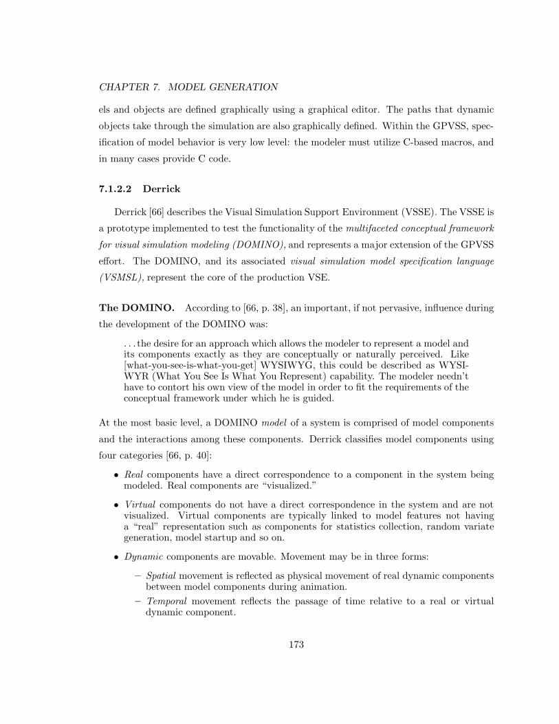
CHAPTER 7. MODEL GENERATION
els and objects are defined graphically using a graphical editor. The paths that dynamic
objects take through the simulation are also graphically defined. Within the GPVSS, spec-
ification of model behavior is very low level: the modeler must utilize C-based macros, and
in many cases provide C code.
7.1.2.2 Derrick
Derrick [66] describes the Visual Simulation Support Environment (VSSE). The VSSE is
a prototype implemented to test the functionality of the multifaceted conceptual framework
for visual simulation modeling (DOMINO), and represents a major extension of the GPVSS
effort. The DOMINO, and its associated visual simulation model specification language
(VSMSL), represent the core of the production VSE.
The DOMINO. According to [66, p. 38], an important, if not pervasive, influence during
the development of the DOMINO was:
. . .the desire for an approach which allows the modeler to represent a model andits components exactly as they are conceptually or naturally perceived. Like[what-you-see-is-what-you-get] WYSIWYG, this could be described as WYSI-WYR (What You See Is What You Represent) capability. The modeler needn’thave to contort his own view of the model in order to fit the requirements of theconceptual framework under which he is guided.
At the most basic level, a DOMINO model of a system is comprised of model components
and the interactions among these components. Derrick classifies model components using
four categories [66, p. 40]:
• Real components have a direct correspondence to a component in the system beingmodeled. Real components are “visualized.”
• Virtual components do not have a direct correspondence in the system and are notvisualized. Virtual components are typically linked to model features not havinga “real” representation such as components for statistics collection, random variategeneration, model startup and so on.
• Dynamic components are movable. Movement may be in three forms:
– Spatial movement is reflected as physical movement of real dynamic componentsbetween model components during animation.
– Temporal movement reflects the passage of time relative to a real or virtualdynamic component.
173

CHAPTER 7. MODEL GENERATION
– Logical movements are changes in the logic decision path of a real or virtualdynamic component.
Derrick [66, p. 50] points out that dynamic components move throughout the staticand dynamic structures (see below) of the model. Movement up and down in themodel static hierarchy is via decomposed submodels (see below). Within a submodel,a dynamic component can utilize the resource of a static component. Dynamic com-ponents can also move into decomposed dynamic components and among its membersubdynamic components and base dynamic components (see below).
• Static components are physically at rest (if real) and immovable (whether real orvirtual). Furthermore, these components are permanently within the model, stayingwithin the model boundaries for the duration of model execution.
These model components form model structures. Two types of model structures are
identified: (1) a model static structure, and (2) model dynamic structures. Only one model
static structure exists for any model – this structure has the model itself as its root –
although it may be comprised of a hierarchy of simple static structures. A model may have
multiple dynamic structures. Based on these structures, five additional classifications for
model components are defined [66, p. 41]:
• A submodel is the root of a simple static structure with children of zero or moresubmodels and zero or more static objects.
• A static object is the most basic model component of interest in a simple static struc-ture and, as such, cannot be decomposed.
• A dynamic object is the dynamic model component which is the basis (root) for modeldynamic structures and is decomposable.
• A subdynamic object is the root of a simple dynamic structure and can be decomposedinto zero or more subdynamic objects and zero or more base dynamic objects.
• A base dynamic object is the most basic model component of interest in a simpledynamic structure and cannot be decomposed.
According to Derrick [66, p. 41], the choice to represent a system component which
is static as a submodel or static object is based primarily on the expected need for a
decomposition point in the model hierarchy.1
1Derrick [66, p. 42] observes that the greatest flexibility in development is retained by modeling systemcomponents as submodels. However, he notes, “other considerations related to visualization/animationrequirements could dictate otherwise.”
174

CHAPTER 7. MODEL GENERATION
Model definition. Under the DOMINO, modelers identify class information such as
attributes, and inheritance hierarchies. Model decomposition points are identified and a
background image is associated with each. These background images, called layouts, provide
the visual landscape over which the dynamic objects travel. A set of images is defined for
each class. Each component within the layout image is identified by graphically binding the
image portion corresponding to the component.
Dynamic object movement between or among model components is specified for each
layout by the creation of roadways or paths. These paths connect the model components
that exist within each layout. Connectors are also created within the layouts to facilitate the
movement of dynamic objects, both into (entry connectors) and out of (exit connectors) the
layout, relative to higher levels. Top-level layouts (for the model and decomposed dynamic
objects), therefore, do not have connectors.2
Interaction points, or interactors, are created which permit dynamic object interaction
with static and base dynamic objects. During animation, dynamic objects are said to move
into decomposable components and to non-decomposable components.
The spatial description of a layout’s image which includes designating model compo-
nents, connectors, interactors and paths is called a layout definition. Each layout image
must have a layout definition. Besides layout definitions, a modeler must also state the
explicit rules governing component behavior. The mechanism for this is described below.
Model specification. The behavior of model components is described using an English-
like specification language called the visual simulation model specification language (VSMSL).
According to Derrick [66, p. 144] the VSMSL, “enables modelers to specify model dynamics,
[and] the rules for component interaction, at a high level.” The VSMSL is utilized in three
types of “logic specifications” under DOMINO [66, p. 70]:
• Supervisory logic. Models built with supervisory logic are machine-oriented. Thesupervisors (machines) are the principle influencers for model execution. The dy-namic objects (material, transactions) are manipulated and moved from componentto component.
• Self logic. Self logic is attached to a dynamic object which executes and determinesits own destiny. Models built entirely around self logic are called material-oriented.
2Movement downward from a level must be directed toward the entry connector at the lower level.
175

CHAPTER 7. MODEL GENERATION
• Method logic. Logic attached to a component class and activated by sending a messageto an owning component in the class.
The VSMSL contains twenty-five statement types supporting a wide variety of behavior
ranging from attribute assignment, to component movement, to display manipulation. In
VSMSL, each reference to a model component includes a reference to its type (e.g. submodel,
static object, dynamic object, subdynamic object, base dynamic object). The language
provides abbreviations, sm, so, do, sdo and bdo for these types. Figure 7.1 contains a
VSMSL description (in supervisory logic) of a queue for a block within a traffic intersection
example similar to the one given in Chapter 6. The figure is taken from [66], and is given
here simply to provide an indication of the nature of the VSMSL. For a complete description
of the VSMSL and the DOMINO, refer to [66].
7.1.2.3 Evaluation
A discussion of the VSSE (as supported by DOMINO and the VSMSL) and the philos-
ophy of this research effort is warranted. Firstly, does the VSSE fit within the structure
of a next-generation framework as presented in Chapter 3? The answer is: not directly.
The philosophy adopted here is that visualization of a simulation model is merely one of
a wide variety of implementation options. Iconic forms may indeed be useful for model
development (see the discussion in Chapter 3), but they need not necessarily correspond
to a given set of animation requirements or forms. When animation of the model is not
a project objective (and admittedly, this may be a rare occurrence), no animation-related
information should be required during model development. The DOMINO and the VSMSL
tightly couple model development to a particular implementation detail: animation.3 As
such, they are incongruous with the philosophy espoused in this effort. Two additional
observations may be made regarding the DOMINO and VSMSL:
• The VSMSL, while English-like in nature and expressive enough to represent a widevariety of behaviors, is in some respects at a lower level than many SPLs. Considerthe VSMSL excerpt given in Figure 7.1. The code:
3This coupling is largely a function of the philosophy of graphical model development underlying theDOMINO.
176

CHAPTER 7. MODEL GENERATION
– BLOCKQUEUE SUBMODEL CLASS SUPERVISORY LOGIC
– *********************************************
– * If there are others waiting or the blockspace is busy, join the queue and
– * wait until first in line and blockspace is idle.– *********************************************
if attr numberWaiting of this sm is> 0 or
attr status of so blockSpace is BUSY@ then
begin
add 1 to attr numberWaiting of this sm;put attr numberWaiting of this sm into holdingVar;
put sys attr ident of this do into
attr vehicleList[holdingVar] of this sm;
engageIn waiting until attr vehicleList[1] of this sm issys attr ident of this do and attr status of so blockspace is IDLE@;
– Reset every vehicle’s position in the queue
put attr numberWaiting of this sm into holdingVar;
subtract 1 from holdingVar;
repeat with i = 1 to holdingVarbegin
put i+1 into dynObjId;
put attr vehicleList[dynObjId] of this sm into
attr vehicleList[i] of this sm
end;subtract 1 from attr numberWaiting of this sm
end
– *********************************************
– * Otherwise, proceed immediately through queue.
– *********************************************
Figure 7.1: Supervisory Logic for a BlockQueue in VSMSL.
177

CHAPTER 7. MODEL GENERATION
add 1 to attr numberWaiting of this sm;put attr numberWaiting of this sm into holdingVar;put sys attr ident of this do into
attr vehicleList[holdingVar] of this sm;
merely implements an enqueue operation. Dequeueing is specified using:
put attr numberWaiting of this sm into holdingVar;subtract 1 from holdingVar;repeat with i = 1 to holdingVarbegin
put i+1 into dynObjId;put attr vehicleList[dynObjId] of this sm into
attr vehicleList[i] of this smend;subtract 1 from attr numberWaiting of this sm
Some higher-level constructs should be provided to support these common mecha-nisms.
• The requirement that the possible paths of dynamic objects must be a priori deter-minable limits the classes of systems that can be animated. The static path paradigmis suitable for manufacturing systems, and networks, but less suitable for systems suchas a colliding pucks (see Chapter 6) or a typical military simulation – through whichtargets may travel and are intercepted at any point in a three-dimensional space. Toanimate systems such as these, a preferred approach is to describe the movement ofmodel objects in terms of a model coordinate system. Movements in the model maythen be translated into a display coordinate system for animation.
Despite the obvious differences in the philosophy of this approach and that of the VSSE
effort, the VSSE investigation has contributed significantly to the theory of visual simu-
lation, and simulation modeling methodology as well. Conceivably, minor changes in the
DOMINO and VSMSL could produce an approach suitable for incorporating visual imple-
mentations within the general framework described in Chapter 3. Certainly, the lessons
learned from the VSSE effort must be recognized in any framework that supports model
animation as a project objective.
7.2 New Directions
Despite the existence of the fully functional Page prototype, the development given in
Chapter 6 is accomplished without automated assistance. The two primary reasons for this
are:
178

CHAPTER 7. MODEL GENERATION
1. The platform hardware for the prototype is tenuous, and has been unsupported bythe manufacturer for several years. Porting the prototype to a new platform wouldrequire considerable effort, and has been deemed a low priority for this research effortin light of the second motivation.
2. The desire to permit the development of this research to be unbiased relative to priorefforts and conclusions.
Thus, the following discussion adopts the perspective of a modeler who has worked directly
in the Condition Specification, without automated assistance. Based on these experiences,
some thoughts are given regarding new ways of coercing a CS from a modeler. First, a
discussion of the attribute-oriented approach to model specification provided by the Barger
and Page prototypes.
7.2.1 Attribute-oriented development
Both the Barger and Page model generators encourage model specification by starting
at the leaves of the model development tree – the attributes. An attribute is selected,
a value change is described, and a condition is associated with that value change. The
motivation for, and observation resulting from, these two efforts is that by causing a modeler
to describe model behavior in this fashion, the specification is quickly “fleshed out,” i.e. the
value changes of a single attribute are typically described in a consecutive manner. This
results in the identification of several model conditions. For typical models, the entire
“condition structure” can be generated from the value changes of just a few (typically,
status transitional) indicative attributes.
However, the question must be asked: does this conform to a “natural” view of model
behavior? That is, when one envisions an object-based model, does the first thought regard-
ing model behavior center around an attribute value change? For some modelers, perhaps,
but certainly not for all. The models in Chapter 6 are specified in the CS using an action
cluster-oriented perspective. Modelers may also prefer other, more traditional, conceptual
frameworks. Some alternative approaches for model generation under the CM/CS based on
the experience gained from Chapter 6 are described below.
179

CHAPTER 7. MODEL GENERATION
7.2.2 Action cluster-oriented development
When a modeler envisions model behavior, the picture may take the form, “when this
occurs, that also occurs.” When the CS is the language of discourse – and the modeler is
working at the CS level – this phenomenon produces an action cluster-oriented depiction of
model behavior. In traditional CFs, and languages supporting these CFs, this phenomenon
might describe an event or activity.4 Interestingly, even when the CS is the target language,
a modeler familiar with traditional CFs will likely identify those conditions which represent
the “root” condition of an event or activity. Consider the situation depicted in Figures 6.7
and 6.8. These figures represent an end-of-service event at the JESS for the MVS model
and the corresponding action clusters. A modeler working in the CS may think of the when
alarm condition first, and mentally lump all the actions from the event into the action
cluster for that condition. Only upon recognizing that a “sub-condition” is present will the
decomposition given in Figure 6.8 be accomplished. This observation illustrates that the
CS, while independent of traditional CFs, does not directly provide a CF facilitating model
development at the highest levels. Still, an action cluster-oriented development could be
helpful. Two different approaches are evident.
7.2.2.1 Action cluster-oriented dialogue.
A dialogue-based model generator for the CS, such as those of Barger and Page, could
readily permit the model to be constructed in an action cluster-oriented fashion. The
dialogue would merely involve the primary identification of conditions with a secondary
association of actions. A more interesting possibility is the use of the action cluster incidence
graph (ACIG) as a basis for graphical development.
7.2.2.2 A graphical approach.
Historically, the ACIG has been constructed from the textual CS representation, and
has functioned solely as a platform for model analysis. However, this incidence graph could
be utilized to foster model development in an action-cluster oriented approach.
4If the modeler naturally views the system using a process view then these events relate to a particularmodel object.
180

CHAPTER 7. MODEL GENERATION
A model generator could provide an iconic interface through which an ACIG might be
constructed. For example, a modeler could create a set of nodes, each identified by a name
or perhaps number. Exploiting iterative refinement, a modeler could “click on” a node and
be given the opportunity to describe the condition and associated actions. When “sub-
conditions” become apparent, the node is decomposed. A modeler might be permitted
to connect any two nodes, irrespective of establishing the criteria for connection, using
solid or dashed arcs. The system could easily identify all unsubstantiated connections, as
well as automatically generating connections between nodes based on the rules for ACIG
construction. The ACIG simplification routines identified by Puthoff [194] could also be
incorporated.
7.2.3 Traditional world view-oriented development
As observed above, even when the CS is the target language, model development is
often facilitated by adopting a traditional world view. Overstreet illustrates how a CS may
be transformed into a specification adopting either the event scheduling, activity scan, or
process interaction world views. Overstreet also postulates that an equivalent CS can be
constructed for any model specification in any programming language [178, p. 247]. While
the veracity of this statement is difficult to assess, certainly any model specification that
conforms to the Conical Methodology can be transformed into an equivalent CS, regardless
of its CF.
Similar to the incidence graph-based approach described above, a model generator could
be constructed which provides CM-oriented variants of event graphs, process graphs, or
activity diagrams which could be used to generate a CS.
181

Chapter 8
MODEL ANALYSIS AND EXECUTION
For one thing, they used computers constantly, a practicetraditional mathematicians frowned on. For another . . .theyappeared to care that their mathematics described somethingthat actually existed in the real world.
Michael Crichton, Jurassic Park
A set of requirements for a next-generation modeling framework is proposed in Chap-
ter 3. An abstraction that implies model development through transformation is also pre-
sented. The basic tenets of modeling methodology stipulate that the overriding objective of
simulation is producing a correct decision. Thus the hierarchy of representations suggested
by the abstraction must support this objective. As recounted in Chapter 3, history indi-
cates a strong correlation between the correctness of the decision and the correctness of the
model upon which the decision is based.
For this research effort, the Conical Methodology has been suggested and evaluated as
a suitable methodology to support a next-generation modeling framework. The objective
of correctness is facilitated (in part) through the provision of high-level implementation-
independent descriptions of the model. These descriptions evolve through a series of refine-
ments until an executable model suitable for a given set of implementation requirements
is produced. The nature of the model evolution, and the level of automatability is, how-
ever, largely a function of the representational forms, the target implementation, and its
concomitant level of maturity as a technology.
The focus of this research in terms of model representation has been at the middle level
of the framework. The Condition Specification is proposed as an intermediate represen-
182

CHAPTER 8. MODEL ANALYSIS AND EXECUTION
tational form for model diagnosis. The implications of this language choice for envisaged
higher-level representations are evaluated in Chapters 6 and 7. In this chapter, the relation-
ship between the CS and lower-level forms is investigated. Generating an executable model
from a CS representation may be affected in two ways: (1) translating the CS representation
into an (several) appropriate implementation language(s), or (2) directly implementing the
CS representation. Addressing the first approach requires the identification of a specific
set of implementation requirements. As suggested by Figure 3.4, the number of possi-
ble combinations of implementation requirements is considerable. The objectives of this
research effort favor broadness of concept and generality of solution. Therefore, the de-
velopment of this chapter focuses on the area where support is potentially most general:
directly implementing a CS representation. Note that translating the CS into a variety of
implementation languages fulfills the transformational hierarchy using a narrow-spectrum
approach (see Chapter 3). Defining methods for directly implementing the CS effectively
widens the spectrum of the language. Both approaches merit investigation, even beyond
that possible in the limited scope of this effort. The groundwork is laid here with a precise
characterization of the semantics of a CS transition specification.
8.1 A Semantics for the Condition Specification
Overstreet’s characterization of a model implementation is reviewed in Chapter 5. If
A(M, t) is a model attribute set for a model specification M at time t. A model specification
is a model implementation if,
1. For any value of system time t, A(M, t) contains a set of state variables.
2. The transition function describes all value changes of those attributes.
Thus, if “system variables” have been added to the object specification set so that A(M, t)
always contains a state set, then the transition description must contain a complete descrip-
tion of how these additional attributes change value. The model implementation serves as
the basis for model execution. The nature of the implementation of a simulation model
varies according to the representational mechanism, and its associated semantics. In this
section, the existing CS semantics are evaluated and, where necessary, re-stated to facilitate
the more definitive mid-level role (in either a narrow-spectrum or wide-spectrum context)
intended for the language within this research effort.
183

CHAPTER 8. MODEL ANALYSIS AND EXECUTION
8.1.1 Interpretation of a condition-action pair
The basic element of a CS is the condition-action pair (CAP). According to Over-
street [178, p. 89]:
The semantics of a CAP are straightforward: whenever the condition is met inthe model, the specified action takes place.
For reasons explicated in the subsequent development of concepts, the semantics of a CAP
adopted here are stated as follows:
The action of a CAP may occur only if the corresponding condition is true.
8.1.2 Interpretation of an action cluster
As outlined in Chapter 5, CAPs with identical conditions form action clusters (ACs).
Overstreet [178, p. 70] asserts:1
In interpreting a [model specification] MS, each CAP is to be treated as a “while”structure rather than an “if” structure. The difference is this: as an “if” theactions of the CAP would occur exactly once when the condition is met; as a“while” the actions repeat until the condition is no longer met.
The motivation for choosing a while-semantics is to accommodate an envisaged clock update
policy: the clock is only updated when all model conditions are false. Thus, when a condition
becomes true, it remains true until a specific action causes the condition to become false. For
determined action clusters (DACs), the while-semantics is accommodated by implication,
i.e. the alarms are assumed to “go off” only once. Overstreet [178, p. 280] states that for
each contingent action cluster (CAC):
at least one output attribute should also be a control attribute for the CAC.. . .Recall that the interpretation of a CAC is a “while” construct rather than an“if.” If the CAC cannot potentially alter the condition, an infinite loop results.To eliminate the infinite loop, it is not sufficient that some other AC can occur inthe same instant as the CAC which can alter the value of the CAC’s condition.For if this were true, the CS would contain unresolved order dependencies.
The diagnostic technique of action cluster completeness (or determinancy, see Chapter 5)
is defined to detect the presence or absence of these infinite loops under this semantics.
1In this passage Overstreet refers to a CAP, but actually intends AC.
184

CHAPTER 8. MODEL ANALYSIS AND EXECUTION
Whenever thisEvent happens
if x = 10 then
y := y + 1
if z thenp := 2
if q then
r := 3
WHEN ALARM(thisEvent):
B$1 := true
B$1 AND x = 10:y := y + 1
B$2 := true
B$3 := true
B$1 := false
B$2 AND z:
p := 2
B$2 := false
B$3 AND q:
r := 3B$3 := false
Figure 8.1: An Event Description with Nested Logic and the Corresponding Action Clusters.
A strict while-semantics, and the associated requirement that the intersection of the out-
put attribute and control attribute sets for any CAC be nonempty, is problematic because
these requirements presuppose that every AC is always a candidate for execution.2 This fact
is readily seen when considering the problem of generating a CS from higher-level forms.
Consider the situation illustrated in Figure 8.1. Here a simple event description consisting
of some nested logic is presented. Also given are the action clusters that might be generated
from this event description using a procedure similar to that described in Chapter 6. Note
the “overhead” in terms of assignments to Boolean variables necessary to satisfy the crite-
rion for action cluster completeness. Clearly this technique could easily become “messy”
for large models and complex condition structures. While the manipulation of additional
Boolean variables may not inhibit automated translation, a significant encumbrance may be
introduced viz. the human understanding of the CS. Figure 8.1 demonstrates that an event
description (at some arbitrarily high level of representation) may contain many conditions,
each of which determines one or more actions. However, these actions need not necessarily
affect the value of their “owning” condition. Some conditions (e.g. x = 10) may remain true
2Here execution refers to the evaluation of the condition on the AC, followed, if the condition is true, bythe performance of the actions given by the AC.
185

CHAPTER 8. MODEL ANALYSIS AND EXECUTION
after the body of the event routine is exited. An important recognition is that in the case
of Figure 8.1, the three CACs must always be coincident with the determined AC. If the
determined AC is not a candidate for execution at some point in a model implementation,
then the truth values of the conditions on the coincident CACs are irrelevant.
Based on the above observation (and in order to support the model of computation
defined subsequently) the semantics of an AC are revised within the context of this research
effort:
Whenever the condition is tested, if the condition is true the associated actionsoccur.
The ordering of actions in an AC is not stipulated. Overstreet proves that determining an
(inter-AC or intra-AC) ordering dependence among arbitrary model actions is undecidable
(see Chapter 5). For general purposes, the actions of an AC may be regarded as sequential,
given some modeler-specified ordering. However, for certain implementations, e.g. those
requiring the exploitation of parallelism, other interpretations may be useful.
8.1.3 Interpretation of action cluster sequences
The execution of a CS on a hypothetical machine may be described in terms of a sequence
of action clusters. The first action cluster in the sequence is the initialization AC, and
the last, termination. Linking initialization and termination is a collection of time-based,
state-based and mixed action clusters. Since any CS containing mixed action clusters may
be transformed into an equivalent CS containing only time-based and state-based action
clusters ([178, p. 215]), the action cluster sequence may be viewed as containing only DACs
and CACs. Overstreet [178, p. 193] observes that this sequence forms a chronology of model
actions as depicted in Figure 8.2. The figure illustrates an action sequence graph (ASG).
An ASG provides similar information to an ACIG except that an ASG connotes the actual
causal relationships resulting from some execution of the CS (on a hypothetical machine).
A formal relationship between the two graphs is established below.
The ASG in Figure 8.2 depicts a trajectory of model execution at some point in sim-
ulation time subsequent to model initialization. State changes occur as the result of a
time-ordered execution of determined action clusters.3 Coincident in (simulation) time
3Here time refers to simulation time.
186

CHAPTER 8. MODEL ANALYSIS AND EXECUTION
timeD D D D D
C C
C
CC
C C
C
C C
CC
C
C
C
D
C
Figure 8.2: Action Sequence Graph. Each determined action cluster (D) must be scheduledprior to its occurrence. After model initialization, some dashed arc must lead into each D.Each contingent action cluster (C) may be caused by either a D or a C, but must occur inthe same instant as some D. Thus each instance of a D can cause (directly or indirectly)a “cascade” of Cs in the same instant in the following manner: the D may change thecondition of one or more Cs to true and their actions may change the conditions of otherCs to true, and so on.
with a determined action cluster are zero or more contingent action clusters. Although not
implied by Figure 8.2, determined action clusters may also be coincident in time. This can
occur in two ways: (1) two (or more) alarms are set for the same future value of simulation
time, or (2) an alarm is set to go off “now.” Strict event scheduling paradigms preclude the
latter situation (in terms of events), but the former is always a possibility in any discrete
event simulation model.
Overstreet’s treatment of a semantics for coincident action clusters is incomplete for our
purposes. He states [178, p. 89]:
Note that it is possible for several conditions to be true simultaneously. In thiscase, the actions are considered to occur simultaneously.
Unclear from this statement is whether this rule applies only to a model specification – in
which all the actions may appear to occur, in some sense, simultaneously (at least during
the same instant), or also to model implementation – for which the validity of such a rule
would be difficult to formulate. For this effort, the following semantics for coincident action
clusters is proposed.
187

CHAPTER 8. MODEL ANALYSIS AND EXECUTION
8.1.3.1 Precedence among contingent action clusters
As indicated by the ASG in Figure 8.2, a “cascade” of CACs may follow the execution
of any DAC. This cascade is formed by precedence relationships among CACs for any given
instant of model execution. If a directed path exists in the ASG between ACi and ACj then
ACi precedes ACj for a particular instant since the execution of ACi causes (directly or
indirectly) the execution of ACj . If no directed path between two ACs exists in the ASG,
then an ordering on their execution cannot be established. In this case, if the two ACs
possess read-write or write-write conflicts (see Chapter 9) then the model implementation
may be ambiguous.
8.1.3.2 Precedence among determined action clusters
As previously stated, two or more DACs may be coincident in (simulation) time during
a given model execution. These DACs may appear as “sources” for a cascade of CACs
in the ASG. A sequenced order of execution for the ACs may follow two general patterns:
(1) execute all DACs, followed by all CACs subject to the precedence relationships among
the CACs, or (2) consecutively execute each DAC and its associated CACs. Based on the
translation scheme between the CS and higher-level event-based forms outlined in Chapter 6,
only the latter approach is correct when “mutually interfering” events occur during the same
instant. This distinction is elaborated below.
For purposes of the following discussion, let E1 and E2 be event descriptions in some
high-level model representation adopting an event scheduling world view. We say that E1
and E2 are mutually interfering, denoted E1 1 E2, if: (1) the actions of E1 are conditional
on the occurrence of E2 and similarly the actions of E2 are conditional on the occurrence
of E1, and (2) E1 and E2 occur during the same instant.4 The following are mutually
interfering events.
4Note that this definition may be extended to more than two events. In fact, it may be readily demon-strated that mutual interference (1) forms an equivalence relation.
188

CHAPTER 8. MODEL ANALYSIS AND EXECUTION
Event E1 Whenever A happens
if event B has not occurredduring this instant
do welse
do x
Event E2 Whenever B happens
if event A has not occurredduring this instant
do yelse
do z
If these two events occur simultaneously, then a serial execution produces either the state
resulting from w and z (E1 followed by E2) or the state resulting from y and x (E2 followed
by E1). If a serial ordering of execution is not provided, the results are indeterminate.5
Using the event-AC correspondence illustrated in Chapter 6 the following ACs may be
produced from the event routines E1 and E2.
AC1 when alarm(A):
B$1 := trueA := true
AC2 B$1 and B:
xB$1 := false
AC3 B$1 and not B:
wB$1 := false
AC4 when alarm(B):
B$2 := trueB := true
AC5 B$2 and A:
zB$2 := false
AC6 B$2 and not A:
yB$2 := false
If the execution of action clusters is such that both DACs are executed prior to the CACs,
then the following sequence is possible: AC1, AC4, AC2, AC5. This sequence produces a
state resulting from x and z. Thus, separation of the DACs from their associated CACs
during execution may result in an “interleaving” of events. If these coincident events are
mutually interfering, such an execution sequence is incorrect.
8.2 Direct Execution of Action Clusters Simulation
Based on the semantics given above, algorithms for the direct execution of action clusters
simulations may be defined. Note however, that several properties of interest, such as
5For an historical perspective on the problem of handling simultaneous events refer to [187]. Some issuesinvolving simultaneous events and parallel simulation are presented in [60].
189

CHAPTER 8. MODEL ANALYSIS AND EXECUTION
the precedence relationship among CACs during any instant, have been defined in terms
of the ASG. Since the ASG depicts an actual execution sequence and is neither a priori
determinable nor a general description of any implementation of a given model specification,
its usefulness for algorithm construction is limited. However, the information available in
an ASG, i.e. the causal relationships among ACs during an execution of the CS, is also
provided in the ACIG. Specifically, the ASG depicts a time series of instances of subgraphs
of the ACIG.
8.2.1 Utilizing the ACIG as a model of computation
We begin with a formal proof that each DAC and associated cascade of CACs in the
ASG has a corresponding subgraph in the ACIG. For purposes of the theorem, we say that
an ASG is vertex-contracted if, for every cascade of CACs, all vertices representing different
occurrences of the same AC are contracted into a single vertex.
Theorem 8.1 For any model specification M in the CS and any implementationM ′, if N ′
is a subgraph of a vertex-contracted ASG(M ′) induced by a single DAC and all CACs reach-able from it without passing through another DAC, then N ′ is a subgraph of ACIG(M).
Proof: Let M be a model specification in the CS and M ′ be the implementa-tion of M on a hypothetical machine. Let G′ be the action sequencegraph of M ′ and G be the action cluster incidence graph of M. Forsome DAC, n ∈ G′, let N ′ be the subgraph of G′ induced by n andall CACs reachable from it without passing through another DAC.Suppose N ′ is not a subgraph of G.Case I: V (N ′) ⊆ V (G). Then an AC is executed which does not ap-pear in G. By definition the ACIG contains all model ACs. ThereforeV (N ′) ⊆ V (G).Case II: A(N ′) ⊆ A(G). Then ∃ i, j ∈ M ′ ACi causes ACj but anarc between ACi and ACj does not exist in G. However, for ACi tocause ACj an output attribute of ACi must be a control attributeof ACj . By definition the ACIG contains an arc from ACi to ACj .Therefore A(N ′) ⊆ A(G).Case III: The restriction of ψG to A(N ′) does not yield ψN ′ . This isfalse trivially.The evaluation of all cases leads to a contradiction. Therefore thesupposition must be false and N ′ is a subgraph of G. 2
The proof that a dashed arc in the ASG has a correspondence in the ACIG is trivial.
Thus, Theorem 8.1 establishes that the ACIG for a CS contains the requisite information
190

CHAPTER 8. MODEL ANALYSIS AND EXECUTION
to provide action cluster precedence consistent with the semantics defined in the previous
section. In other words,
the ACIG provides a context for control flow in an implementation of the CS.
Whenever an AC is executed, the only ACs potentially enabled as a result, and therefore
the only model conditions which must be subsequently tested, are given by the arcs in the
ACIG. Algorithms suitable to exploit the information provided by the ACIG are presented
below.
8.2.2 Minimal-condition algorithms
Figures 8.3 and 8.4 present algorithms for direct execution of action clusters (DEAC)
simulations that are described as “minimal-condition.” Minimal-condition implies that
given a completely simplified ACIG as a basis, and using the semantics for a CS defined
above, the number of state-based conditions evaluated upon the execution of any given AC
is minimal. Note that the optimality of these algorithms depends, to a large extent, on
their implementation (as briefly discussed below). Two algorithms are defined. For both
algorithms a list, A, of scheduled alarms is maintained as well as a list of state-based action
clusters, C, whose conditions should be tested within the current context of model execution.
The simplified ACIG provides a list of state-based successors for each AC which is used to
maintain C.Figure 8.3 presents a minimal-condition algorithm for a CS containing mixed ACs.
Efficiently handling mixed action clusters requires a somewhat sophisticated approach. If
σj is a mixed AC and a solid arc exists in the ACIG from AC σi to σj, then let σj ∈ σiS
(the set of state-based successors of AC σi). When a mixed AC is a state-based successor
of an executing AC, only place the mixed AC in C (the list of potentially enabled ACs) if
the AC is in M (i.e. its alarm part has already gone off). When the mixed AC executes,
that AC is removed from both M and C.
Figure 8.4 depicts a minimal-condition algorithm for a CS without mixed ACs. Note
that in both algorithms, executing the termination AC (as either a determined, contingent
or mixed AC) causes an exit from the simulation proper. Note also that an AC may appear
in multiple successor sets. Therefore, an efficient implementation of both algorithms might,
among other things, check for duplicates when inserting into the list C.
191

CHAPTER 8. MODEL ANALYSIS AND EXECUTION
LetA be the ordered set of scheduled alarms.
Let C be the set of state-based and mixed action clusters whose conditions should be tested immediately.
LetM be the set of mixed action clusters whose alarms have “gone off” but whose Boolean conditionhas not been met.
Let σiS be the set of state-based successors for action cluster σi (where 1 ≤ i ≤ | ACs | ).
Initially
∀σi, set σiS (from simplified ACIG)A = C =M = ∅Perform actions given by the initialization AC and state-based successors
Simulate
while (true) do
clock← time given by FIRST(A)
while (clock = time given by FIRST(A)) do
let σa be the AC corresponding to FIRST(A); remove FIRST(A)if (condition on σa is WHEN ALARM) or (condition on σa is AFTER ALARM and Boolean part is true)
perform actions of σaadd σaS to C
while (C = ∅)
remove σc ← FIRST(C)if condition on σc is true
perform actions of σcif σc ∈M, remove σc fromMfor each σi ∈ σcS do
if condition on σi is not mixed then add σi to Cif condition on σi is mixed and σi ∈M then add σi to C
endfor
endif
endwhile
elseadd σa toM
endif
endwhile
endwhile
Figure 8.3: The Minimal-Condition DEAC Algorithm for a CS with Mixed ACs.
192

CHAPTER 8. MODEL ANALYSIS AND EXECUTION
LetA be the ordered set of scheduled alarms.
Let C be the set of state-based clusters whose conditions should be tested immediately.
Let σiS be the set of state-based successors for action cluster σi (where 1 ≤ i ≤ | ACs | ).
Initially
∀σi, set σiS (from simplified ACIG)
A = C = ∅Perform actions given by the initialization AC and state-based successors
Simulate
while (true) do
clock← time given by FIRST(A)while (clock = time given by FIRST(A)) do
let σa be the AC corresponding to FIRST(A); remove FIRST(A)
perform actions of σaadd σaS to C
while (C = ∅)
remove σc ← FIRST(C)
if condition on σc is true
perform actions of σcadd σcS to C
endifendwhile
endwhile
endwhile
Figure 8.4: The Minimal-Condition DEAC Algorithm for a CS without Mixed ACs.
193

CHAPTER 8. MODEL ANALYSIS AND EXECUTION
Another factor relating to the execution efficiency of these algorithms is the potential
loss of structure information within an ACIG. For example, if a high-level representation
provides a case, or switch, selector, then the ACIG produced from this description contains
an AC, say ACi with multiple, say n, state-based successors. The semantics provided by
the higher-level representation, permit determination that a singular successor AC exists
whose actions are enabled by the exeution of ACi. However, the ACIG does not reveal
this information. Thus, during execution each condition is tested. If these conditions are
suitably complex, the efficiency of this approach may be substantially inferior to a target
language where an optimizing compiler may provide such mechanisms as lazy evaluation
and short circuiting (see [5]). Conceivably, the ACIG could be annotated to indicate these,
and similar, types of situations. Such details, however, are beyond the scope of this research
effort.
8.3 Provisions for Model Analysis and Diagnosis
Clearly, a major strength of the CS is its facilitation of model analysis and diagnosis, a
capability that distinguishes it from extant simulation languages – both specification and
implementation. Model analysis is considered to include all operations on a model represen-
tation made with the intent to extract information regarding properties or characteristics
of the model representation. Model diagnosis is model analysis with the objective of estab-
lishing the truth of some assertion(s) regarding the model representation or assisting the
modeler in resolving potential questions regarding the representation. Section 8.3.1 exam-
ines the impact of the proposed CS semantics on the extant provisions for model diagnosis.
The remaining sections describe some issues in model analysis raised by this research effort.
8.3.1 Impact of proposed semantics on extant diagnostic techniques
The diagnostic techniques given in Table 5.4 are re-stated here and assessed in terms of
the proposed CS semantics. The techniques are divided into three categories: (1) analytical
techniques, (2) comparative techniques, and (3) informative techniques. The definitions
below are adapted from [163, 164, 194].
194

CHAPTER 8. MODEL ANALYSIS AND EXECUTION
Analytical techniques. Analytical techniques indicate the presence or absence of specific
properties in a model specification. Eight analytical techniques are defined in [163].
• Attribute utilization. An attribute is utilized if the attribute affects the value ofanother attribute. Utilization cannot be guaranteed, only estimated. If an attributeappears in as a control attribute or input attribute in some action cluster, the attributeis considered utilized (even though the action cluster itself may never be utilized). Thistechnique is unaffected by the proposed semantics.
• Attribute initialization. All model attributes should be given an initial value beforethey are used. If an attribute is an output attribute of the initialization AC thenattribute initialization is guaranteed.6 Otherwise attribute initialization may onlybe estimated. However, if the attribute has a zero in-degree in the ACAG, the at-tribute is guaranteed to be uninitialized. This technique is unaffected by the proposedsemantics.
• Action cluster completeness. Referred to as action cluster determinacy in [194], thistechnique determines if the intersection of the output attribute and control attributesets for any action cluster is nonempty. The proposed action cluster semantics andresultant DEAC algorithms obviate this technique.
• Attribute consistency. The usage of an attribute should be consistent with its type.This technique is unaffected by the proposed semantics.
• Connectedness. When the initialization AC and its arcs are removed from the ACIG,if the remaining graph has multiple components this typically (although not necessar-ily) indicates an incomplete model specification. This technique is unaffected by theproposed semantics.
• Accessibility. An action cluster, ACj , is accessible if there exists a directed path inthe ACIG from the initialization AC to ACj . This technique is unaffected by theproposed semantics.
• Out-complete. A model specification is out-complete if the only AC in the simplifiedACIG with an out-degree of zero is the termination AC. This technique is unaffectedby the proposed semantics.
• Revision consistency. This technique establishes the degree of consistency in the ACIGbetween model revisions. This technique is unaffected by the proposed semantics.
Comparative techniques. Comparative techniques provide relative measures of a model
representation characteristic, i.e. these measurements may only be assigned meaning in the
comparison of model specifications. Three comparative techniques have been proposed.
6If the attribute is also an input attribute of the initialization AC, statement ordering must also beconsidered.
195

CHAPTER 8. MODEL ANALYSIS AND EXECUTION
• Attribute cohesion. The degree to which attribute values are mutually influenced.Powers of the AIM (see Chapter 5) indicate attribute cohesion. This technique isunaffected by the proposed semantics.
• Action cluster cohesion. The degree to which action clusters are mutually influenced.Powers of the ACIM (see Chapter 5) indicate action cluster cohesion. This techniqueis unaffected by the proposed semantics.
• Complexity. The complexity of a model specification may be assessed in terms of itselegance as a communicative model (psychological complexity) or perhaps in terms ofits transformational relationship to a programmed model (computational complexity).The effect of the proposed semantics on a complexity measure depends upon themeasure. Wallace’s control and transformation metric [238], for example, relates onlyto the structure of the ACIG and to the classification of attributes, and is unaffectedby the proposed semantics.
Informative techniques. Informative techniques provide measurements of quantifiable
model specification properties. However, these measurements typically demand interpreta-
tion and inference on the part of a modeler or analyst to be effective. Three informative
techniques have been identified.
• Attribute classification. Attributes may be classified as: (1) input, (2) output, or (3)control. This technique is unaffected by the proposed semantics.
• Precedence structure. An indication of a mandated ordering on the execution of actionclusters for any given instant. The proposed semantics provide explicit rules forgenerating precedence structures.
• Decomposition. Typically applied to the ACIG, a model specification may be alter-natively composed (see Chapter 5). This technique is unaffected by the proposedsemantics.
8.3.2 On multi-valued alarms
Overstreet permits an alarm to be set for multiple values. Ostensibly, multi-valued
alarms provide a substantial amount of flexibility in model description. However, if the
condition on an alarm is an after alarm, the possibility of multiple values may potentially
lead to an ambiguity in the model implementation. Consider the ACIG fragment illustrated
in Figure 8.5. If x becomes 5 between time 10 and 20, then two “instances” of the after
alarm AC occur. If x doesn’t become 5 until time 30, then only one occurrence of the
after alarm AC is produced.
196

CHAPTER 8. MODEL ANALYSIS AND EXECUTION
SET ALARM(arrival, 10)SET ALARM(arrival, 20)
AFTER ALARM(arrival AND x = 5):
x := 5
Figure 8.5: An Improper Usage of Multi-Valued Alarms.
By simple extension of Overstreet’s arguments involving the inherent limitations of static
analysis on a CS, no technique can be defined to automatically detect this type of misuse of
multi-valued alarms. However, a modeler should be wary of this possibility when utilizing
the after alarm construct.
8.3.3 On time flow mechanism independence
In his 1971 paper, Nance [152] illustrates that, counter to a widely held belief, next-event
time flow is not always computationally superior to fixed-time. He further observes [152, p.
72]:
The concept of a continuum of time flow algorithms seems warranted . . .Atseparate ends of the continuum are the fixed time and next-event methods, whichare simply algorithms themselves. For any specific simulation application, themost efficient algorithm may be anywhere along the continuum with its locationreflecting the degree to which it reflects the characteristics of either pole.
When this position is logically resolved with Nance’s subsequent writings on modeling
methodology, the role of the time flow mechanism becomes that of an implementation
detail – which should be separable from model representation at high levels of description.
In defining the CS, Overstreet enunciates a congruous philosophy [178, p. 79]:
Since system time is a model input attribute, the model contains no descriptionof how it changes value (except for its initialization). Thus a choice of timeadvance mechanism can be based on analysis of the model specification. Eithera fixed or varying time increment could be used, (for that matter the model couldbe run in “real time”); the model specification does not dictate the choice.
197

CHAPTER 8. MODEL ANALYSIS AND EXECUTION
Because of the results reported by Nance, the concept of a time flow mechanism-independent
representation is appealing. However, as indicated in the development below, the CS,
while supporting both the next-event and fixed-time mechanisms, does not provide an
independence from their selection.
Consider a very simple version of the Pucks model described in Chapter 6 in which a
single puck is placed on a frictionless table. Assume that an initial position and velocity are
specified and the system is to be simulated for a specific number of collisions after which the
final position of the puck is reported. As illustrated in the development of the Pucks model
in Chapter 6, the description of model behavior is dependent upon a particular view of time
flow. In other words, model behavior may be described along two basic lines (the poles
of Nance’s continuum): (1) schedule the next collision, collide, schedule the next collision,
collide, etc. or (2) travel for a certain period of time, see if a collision occurred, travel some
more, see if a collision occurred, and so on. Figure 8.6 contains two CS specifications for
this model and their respective action cluster incidence graphs. The specification for each
reflects a different view of time flow, one next-event, and the other fixed-time.
Thus, the evidence suggests that the CS does support a variety of time flow mecha-
nisms. However, the CS is not independent of the underlying time flow mechanism; the
manipulation of alarms in the CS directly reflects a perception of time flow. The assertion
is made here, but not proven, that any operational representation (see [8]) is inextricably
bound to a perception, if not a precise description, of the underlying time flow mechanism.
Conceivably, a definitional representation defining a model more in terms of a set of objec-
tives and rules, may provide the true independence from time flow for which Nance clearly
demonstrates the need.
8.4 Summary
In this chapter, issues in model analysis and execution within the CM/CS approach are
investigated. The semantics of the CS are refined to provide support for model execution.
Based on a model of computation provided by the ACIG, an implementation structure
referred to as a direct execution of action clusters (DEAC) simulation is defined, and two
DEAC algorithms are presented. The extant provisions for model analysis and diagnosis in
the CS are evaluated with respect to the refined semantics (and the syntax extensions from
198
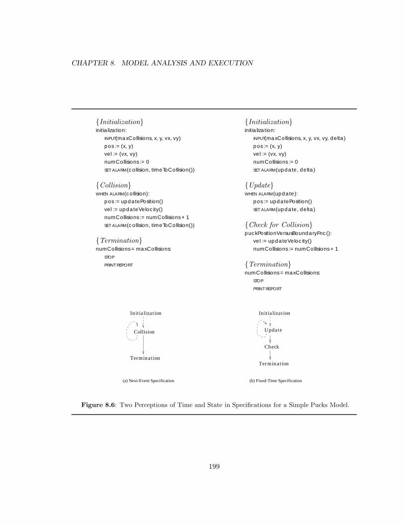
CHAPTER 8. MODEL ANALYSIS AND EXECUTION
Initializationinitialization:
INPUT(maxCollisions, x, y, vx, vy)
pos := (x, y)vel := (vx, vy)
numCollisions := 0
SET ALARM(collision, timeToCollision())
CollisionWHEN ALARM(collision):
pos := updatePosition()
vel := updateVelocity()
numCollisions := numCollisions + 1
SET ALARM(collision, timeToCollision())
TerminationnumCollisions = maxCollisions:
STOP
PRINT REPORT
Initializationinitialization:
INPUT(maxCollisions, x, y, vx, vy, delta)
pos := (x, y)vel := (vx, vy)
numCollisions := 0
SET ALARM(update, delta)
UpdateWHEN ALARM(update):
pos := updatePosition()
SET ALARM(update, delta)
Check for CollisionpuckPositionVersusBoundaryFnc():
vel := updateVelocity()
numCollisions := numCollisions + 1
TerminationnumCollisions = maxCollisions:
STOP
PRINT REPORT
(a) Next-Event Specification (b) Fixed-Time Specification
Initialization
Collision
Termination
Initialization
Update
Check
Termination
Figure 8.6: Two Perceptions of Time and State in Specifications for a Simple Pucks Model.
199

CHAPTER 8. MODEL ANALYSIS AND EXECUTION
Chapter 6).
The chapter concludes with an evaluation of the CS as a time-flow-mechanism-independent
representation. We demonstrate that the use of the alarm construct in the CS must reflect
some view of the passage of time. We postulate that this problem exists for any operational
specification language.
200

Chapter 9
PARALLELIZING MODEL EXECUTION
For the earliest system of philosophy . . .was like unto one ar-ticulating with a stammer, inasmuch as it was new as regardsfirst principles, and a thing the first in its kind.
Aristotle, The Metaphysics
One of the underlying themes of this research is that the preeminent role of decision
support within the context of simulation persists under any particular set of study require-
ments. By extension, the modeling practices that facilitate the development and assessment
of model correctness must be preserved within any modeling approach. The observations of
Nance and Sargent which provide the foundation for the requirements of a next-generation
modeling framework (Chapter 3) adhere to this philosophy. However, the simulation litera-
ture is replete with examples of approaches where recognition of the fundamental nature of
simulation as a decision support tool is missing, or unstated. As discussed in the develop-
ment of the colliding pucks model in Chapter 6, parallel discrete event simulation supplies
several such examples.
In this chapter, the Conical Methodology/Condition Specification (CM/CS) approach
to model development is evaluated in terms of its provisions for incorporating parallelism
into model execution. A characterization of the inherent parallelism available in a CS model
specification is given. This characterization is based on Nance’s delineation of the time and
state relationships in a simulation model. Algorithms suitable to permit the exploitation
of parallelism within the execution of an ACIG-based simulation model are presented. To
preface the development of these algorithms, Section 9.1 contrasts the model development
approach (typically) adopted within parallel discrete event simulation with the philosophy
201

CHAPTER 9. PARALLELIZING MODEL EXECUTION
that guides this research. For completeness of the presentation, a few basic parallel discrete
event simulation concepts are also reviewed.
9.1 Parallel Discrete Event Simulation: A Case Study
Parallel discrete event simulation (PDES) is usually regarded as the method of executing
a single simulation program on multiple processors.1 Typically, PDES refers to simulation
on a multiprocessor – either MIMD or SIMD (see [224]). However, several PDES techniques
stipulate a strict message passing communication scheme and therefore are applicable to
distributed (network-based) approaches. In this chapter, the primary focus is on PDES
techniques suitable for MIMD architectures. Distinctions between parallel computation
and distributed computation are made where appropriate.
9.1.1 A characterization of sequential simulation
The characterization of discrete event simulation commonly held in PDES is rather
narrow – focusing strictly on the implementation requirements. According to Fujimoto [78,
p. 31], “sequential simulators” typically utilize three data structures: (1) the state variables
that describe the state of the system, (2) an event list containing all pending events, and
(3) a global clock that denotes how far the simulation has progressed.2 Model execution
involves the repeated process of removing the event with minimum timestamp, Emin, from
the event list and modifying state variables, and/or scheduling other events as prescribed
by the event routine corresponding to Emin. The process continues until the condition for
termination is met, or until no unprocessed events remain – in which case the simulation is
not well-defined.
Fujimoto notes that in the traditional sequential execution paradigm, selection of the
next event (on the event list) to be processed, Emin, as the one with the smallest timestamp
1Several alternate views of PDES have been proposed, such as the execution of independent replicationsof a single simulation experiment on multiple processors, or parallelization of simulation support routinessuch as the event list. However, the problem of applying multiple processors to a single replication of a givenprogram is viewed as the most general (and difficult) problem.
2In its purest form, the activity scanning world view does not prescribe an event list. The three-phaseand process interaction approaches, however, do include abstractions built upon the event list structure(see [19]).
202

CHAPTER 9. PARALLELIZING MODEL EXECUTION
is crucial. Otherwise, if an event, say Ex, is selected such that Ex modifies one or more
state variables used by Emin, the simulated future may affect the simulated past. Fujimoto
refers to errors of this nature as causality errors.
A defining characteristic of PDES approaches is the need to synchronize proces-sors such that causality in the simulation is preserved.
Nicol and Fujimoto [171] observe that interest in parallel simulation arose first with the
problem of synchronization, and this problem has remained the focus of most research in
PDES for the last 15 years.
The simplest method of processor synchronization is for all processors to perform in
lock-step fashion. These synchronous-time (global clock) approaches, such as the one pro-
posed by Jones [116, 117], are particularly suited for shared-memory multiprocessors and
models in which a large proportion of the model objects are involved in any given event.3
In a typical queueing network simulation, on the other hand, the proportion of model ob-
jects involved in a single event is often quite small. Networks of queues are of fundamental
utility in many areas, such as computer architecture and component design, communica-
tions and manufacturing. Resulting from a combination of their relative importance, and
their general lack of amenability to synchronous-time parallel implementations, an alterna-
tive paradigm has emerged to support the efficient parallel execution of queueing networks.
These asynchronous-time (local clock) approaches fall broadly into two categories: (1) con-
servative, and (2) optimistic. These approaches, or protocols, typically center around a set
of logical processes, one per physical “real-world” process. All interactions between physi-
cal processes are modeled by timestamped event messages sent between the corresponding
logical processes [78]. Each logical process contains a local clock which indicates the pro-
gression, in simulation time, of the logical process. Using this logical process paradigm,
a sufficient condition to guarantee that no causality errors occur in the model is for each
logical process to execute events in nondecreasing timestamp order [78, p. 32].
Unquestionably, the conservative and optimistic asynchronous-time methods have re-
ceived more focus than any other techniques for parallelizing model execution. The con-
sensus among PDES researchers is that if a “general-purpose” parallel discrete event sim-
ulation engine is to be defined, it must be based on an asynchronous-time mechanism. A
3This point is elaborated in Section 9.2.3.
203

CHAPTER 9. PARALLELIZING MODEL EXECUTION
0.6
0.4S1
S2
S3
100
Figure 9.1: A Closed Queueing Network with Three Servers. Server S2 sends a messageto server S1 with timestamp 100.
brief description of the conservative view versus the optimistic view follows. For a detailed
treatment of the underlying concepts in PDES, refer to Fujimoto [78]. Another valuable
source is Nicol and Fujimoto [171]; the authors provide a state-of-the-art survey of research
directions in PDES, dividing these directions into 6 categories: (1) protocols, (2) perfor-
mance analysis, (3) time parallelism, (4) hardware support, (5) load balancing, and (6)
dynamic memory management.
9.1.2 Conservative approaches
The first asynchronous-time algorithms for PDES were conservative algorithms [41, 46].
Conservative algorithms are characterized by the fact that no process executes a message
(event) until a guarantee is given that no message will arrive later in the simulation such that
the simulation time (timestamp) of the new message is earlier than the one just executed, i.e.
events occur locally in strictly chronological (nondecreasing timestamp) order. Accordingly,
processes must block until this guarantee can be met.
Figure 9.1 illustrates a closed queueing network with three servers. In the figure, a
message from S2 is being sent to S1 with timestamp 100. If the last message from S3 was
processed by S1 at time 70, and no other information regarding the time of the next message
from S3 is available to S1, under a conservative protocol S1 must block. S1 blocks since the
possibility exists that S3 may send a message with timestamp between 70 and 100. This
blocking requirement can lead to deadlock in the simulation – for example, if S3 has no mes-
sages left to process, and is therefore waiting for a message from S1. Methods for dealing
204

CHAPTER 9. PARALLELIZING MODEL EXECUTION
with deadlock are the focus for much of the research in conservative PDES. Deadlock can be
avoided through the use of null messages [13, 46] or deadlock can be detected and recovered
from [47, 93]. Other efforts aimed at improving the performance of these basic conservative
mechanisms include using barrier-type synchronization techniques [172], precomputation
within the simulation [168], conservative Time Windows [137], and application-specific op-
timizations [85, 92, 192].
Fujimoto observes that an obvious drawback of conservative approaches is their inabil-
ity to fully exploit the parallelism available in a simulation model [78, p. 39]. If event
dependencies are unknown, event execution must often be serialized, even though parallel
execution of the events would not violate simulation causality.
9.1.3 Optimistic approaches
Optimistic algorithms are characterized by the fact that each process executes events as
they arrive and assumes that events arrive in nondecreasing timestamp order. When causal-
ity is violated, optimistic algorithms rollback and execute the events in proper order. Thus,
in Figure 9.1, under an optimistic protocol S1 would process the message from S2 immedi-
ately upon its receipt. If a message subsequently arrives from S3 with timestamp less than
100, S1 must rollback, undue the effects of any out-of-order events, and re-execute the events
in proper order. On the other hand, if the next message from S3 has timestamp larger than
100, no processing time was “wasted” due to unnecessary blocking. Optimistic algorithms
are not subject to deadlock, since no process blocks during execution, but must ensure that
simulation activity progress forward (in some global sense) so that the simulation eventu-
ally terminates. The most widely recognized optimistic protocol is Time Warp [114, 115]
based on the concept of virtual time [113]. Time Warp has received substantial investigative
research, and considerable effort has been expended to understand and improve the perfor-
mance of the protocol (for examples, see [44, 53, 81, 84, 132]). Recently, other optimistic
protocols have been proposed, these include optimistic Time Window approaches [217, 218],
and Space-Time [49].
Some experiments using optimistic methods have yielded impressive speedups (see [79]).
However, state-saving overheads can significantly degrade the performance of an optimistic
method like Time Warp. Hence, both conservative and optimistic protocols have relative
205

CHAPTER 9. PARALLELIZING MODEL EXECUTION
strengths and weaknesses. No single protocol is ideally suited for all imaginable models
– particularly those whose dynamic behavior is a function of model input. Fujimoto [78]
identifies some criteria for the selection of an implementation algorithm based on system
characteristics. However, these heuristics are insufficient to guarantee algorithm selection
yielding optimal performance, and in some instances utilize properties which are difficult to
quantify. Some other attempts to analyze and quantify the performance bounds of PDES
protocols may be found in [127, 131, 133, 173].
9.1.4 A modeling methodological perspective
In a series of articles published in the Summer 1993 volume of the ORSA Journal on
Computing, several of the leading researchers in parallel discrete event simulation assess
the state of the field. In the lead article, Fujimoto observes that despite many reported
successes in terms of improved performance, PDES has failed to “make a significant impact
in the general simulation community” during the last 15 years of its development [79, p.
228]. Several factors are identified as contributing to this lack of impact, and various
approaches are proposed to make parallel simulation “more accessible to the simulation
community.” Each companion article, [1, 10, 129, 200, 235], acknowledges the acceptance
problem. Fujimoto’s proposals to increase accessibility are critiqued, and several alternatives
are presented.
Abrams [1] suggests that the precipitate cause of the problem is a dichotomy in the
perspectives and priorities of modeling methodologists – the primary purveyors of discrete
event simulation, and parallel programmers – the leaders in parallel discrete event simula-
tion, noting that until these two camps come to terms it is unlikely that PDES will thrive.
Fujimoto [80, p. 247] acknowledges the correctness of this assertion and labels the potential
collaborative attack as a “worthy goal.” Page and Nance [185] elaborate on Abrams’ asser-
tion, and present a view of the parallel discrete event simulation problem from a modeling
methodological perspective. The major themes of that source are summarized briefly here.
9.1.4.1 Observations
If PDES research is contrasted with the modeling methodological perspective outlined in
Chapter 3, differences become evident in two areas: (1) the enunciation of the relationship
206

CHAPTER 9. PARALLELIZING MODEL EXECUTION
between simulation and decision support, and the guidance provided by the life cycle in this
context, and (2) the focus of the development effort.
Life cycle and decision support. Using [12] as a framework for the discussion, Page [183]
characterizes the directions of PDES research as displaying an incognizance of the funda-
mental nature of simulation as a decision support tool, and the importance of the life cycle
as supportive of simulation in all contexts. The opening lines of the response from Chandy
et al. [50] are illuminating:
Discrete event simulation is a vibrant field. It has many subfields. The softwareengineering of simulation is such a subfield, and the “simulation life cycle” is anexample in this subfield. Our paper is focused on a different subfield: parallelsimulation.
These comments present a stark contrast between the philosophies of modeling methodology
that have developed over the past four decades, and a prevalent viewpoint in PDES research.
To suggest that parallel simulation may somehow be divorced from the simulation life
cycle indicates a potentially significant misperception regarding the fundamental nature of
simulation. As Page responds [183, p. 286]:
The simulation model life cycle is most certainly not a topic in any subfieldof discrete event simulation. The simulation model life cycle is the foundationupon which all of discrete event simulation is placed. Everything that is DESflows from the life cycle – be it modeling, requirements analysis, executablerepresentations, verification and validation, or presentation of results to decisionmakers – it all emanates from the life cycle.
The primacy of decision support seems to be often overlooked – or at least regarded as
inconsequential, or as a detail that can be “filled in later” – in PDES research. Perhaps
this perception explains why the big payoff of PDES, the heralds of improved performance,
fall largely on deaf ears in the general discrete event simulation community. To evaluate
the benefits of applying parallelism to simulation solely on the basis of typical evaluative
measures for parallel programs, such as speedup in runtime, is specious – at best. Such a
view casts simulation as merely a piece of code which is run to produce the answer. This
view is overly simplistic. To gain “general” acceptance, PDES research must examine the
methods used to attain execution speed explicitly in terms of their relationship to the central
objective of any simulation: arriving at a correct decision.
207

CHAPTER 9. PARALLELIZING MODEL EXECUTION
Whenever Arrival:
if machine status is failed
set repairman status to busy
schedule end repairelse
schedule arrival at next machine
Whenever Failure:set machine status to failed
Whenever End Repair:
set machine status to operational
set repairman status to idle
schedule next failure for this machineschedule arrival at next machine
Figure 9.2: A Partial Event Description for the Patrolling Repairman Model.
Moving toward the machine. The majority of PDES research has been conducted
with little regard for the role of the conceptual framework within the model development
process. The following quote (from [225, p. 612]) represents a typical (asynchronous-time)
PDES problem description:
We assume the system being modeled consists of some number of physical pro-cesses which interact in some manner. The simulation program consists of acollection of logical processes each modeling a single physical process.
Little distinction between model and program is made, and the paradigms prescribe a
singular perspective: a contrived form of process interaction. This “logical process” view is
characterized as contrived because its definition is motivated more by execution concerns
than by an accurate representation of the physical counterpart. Fujimoto [78, p. 33] notes
that this (logical process) view enables application programmers to partition the simulation
state variables into a set of disjoint states, to ensure that no “simulator event” accesses
more than one state. Such a partitioning permits “minimal” processor synchronization.
Figures 9.2, 9.3 and 9.4 contrast three views of a partial specification (initialization and
termination are omitted) of the patrolling version of the machine interference problem (see
Chapter 6). Figure 9.2 illustrates an event scheduling representation. Figure 9.3 depicts
a process interaction description using the SIMULA concepts activate and passivate, and
Figure 9.4 illustrates a logical process representation of the model. Note the somewhat
convoluted communication structure in Figure 9.4, resulting primarily from the inability of
the repairman to directly examine attributes of a machine (e.g. machine status).
208

CHAPTER 9. PARALLELIZING MODEL EXECUTION
REPAIRMAN:
while true
wait travel time
if status of current machine is failed
set my status to busy
wait repair time
set status of current machine to operationalactivate current machine
set my status to idle
end if
update current machine
end while
MACHINE:
while true
wait until failure
set my status to failed
passivate
end while
Figure 9.3: A Partial Process Description for the Patrolling Repairman Model.
REPAIRMAN:
case message type of:
End Repair::set my status to idle
send travel msg to self (now)
Begin Repair::
set my status to busy
Travel::send arrival msg to next machine
end case
MACHINE:
case message type of:
Arrival::if my status is failed
send begin repair msg to repairman (now)
send end repair msg to self, repairman
else
send travel msg to repairmanEnd Repair::
set my status to operational
send failure msg to self
Failure::
set my status to failed
end case
Figure 9.4: A Partial Logical Process Description for the Patrolling Repairman Model.
209

CHAPTER 9. PARALLELIZING MODEL EXECUTION
The evidence is incontrovertible: in typical PDES approaches, the requirements of a
“logical-process-oriented” implementation are allowed to dictate the conceptualization of
the model itself. Clearly, any such requisite perspective is counter to Derrick’s precepts of
conceptual framework selection, and further, this movement “toward the machine” reverses
that which has taken place in both simulation and software engineering over the several
decades. The conceptual restrictions prevalent within PDES, as well as a penchant for
working from a program view, result in model representations (the programs) that are often
contrived and unnatural descriptions of the system being modeled. Execution requirements
force model perturbations unrelated to the (often unstated) study objectives and the natural
system description that exists in the mind of the modeler. Further, the problems of model
verification and validation as well as those of life-cycle support become greatly exacerbated.
Without a clear picture of the objectives and priorities of the general DES community,
however, these problems remain largely unrecognized. For PDES to realize the desired
level of acceptance in the DES community, performance gains must be achievable without
sacrificing software quality objectives. Existing techniques may well provide this capability;
that remains to be demonstrated. Perhaps this demonstration has been delayed by a lack
of agreement as to its need.
9.1.4.2 Recommendations
Chapter 3 presents a philosophy that prescribes the fundamental nature of simulation,
i.e. what simulation is. Also provided by the philosophy are theories of how simulation
should be applied. The philosophy describes a “modeling methodological” view of sim-
ulation: simulation is a model-centered, problem-solving technique that serves first and
foremost as a basis for decision support. This view is by no means exclusive. The prevalent
treatment of DES by the parallel discrete event simulation community would seem to offer
an example of one alternative.
The argument is made here that the view of discrete event simulation presented in
Chapter 3 largely reflects that of the “mainstream” of DES – for better, or for worse.
Therefore, if PDES seeks to make a broader impact within the general DES community,
then the methods of PDES must be resolved, at least to some degree, with the modeling
methodological view. This resolution might be accomplished in myriad ways; no single
210

CHAPTER 9. PARALLELIZING MODEL EXECUTION
“silver bullet” is evident. Nonetheless, the following list appears to be a logical starting
point:
1. Focus on the model. The move from a program-centered view to a model-centeredview has been documented. Many methodologies and environments for DES pro-vide programming-language-independent forms for model description. Even thoseapproaches that advocate a “program-as-model” description provide architectural in-dependence: the same program is executable on machines with disparate architectures,as long as each machine has the requisite compiler. Without question, any approachto discrete event simulation that ties the modeling task directly to the implementingarchitecture is destined to meet with failure.
2. Consider the simulation study objectives. Many published efforts in PDES demon-strate speedup by changing the model. The tradeoff of speed for accuracy is a legit-imate modeling issue. However, the degree to which model changes are acceptableis a direct function of the objectives of the study. Rarely are these objectives stipu-lated, however, and the reader is often left with questions concerning the validity ofthe resulting program, and by implication, the viability of the approach. With veryfew exceptions, every paper in which a simulation is involved should include a set ofstudy objectives. Changes to the model made in an effort to exact speedup must thenbe addressed in terms of their effect on model validity. Some popular PDES bench-marks such as colliding pucks (see Chapter 6) and sharks world (see [11, 169, 193])are unsatisfactory in this regard.
3. Examine the methods in terms of a given simulation approach. As outlined in Chap-ter 1, discrete event simulation is utilized in a wide variety of contexts. The contextof the model’s usage may influence the suitability of a given approach to obtainingspeedup in execution. For example, if the simulation is used in an evolutionary formto design or optimize a system, then a posteriori analysis and subsequent modifica-tion of code to obtain speedup is likely to be less feasible than in a situation where amodel, once constructed, is run many times with few changes.
4. Examine the relationship of speedup to software quality. How does the method used toexact speedup affect the model in terms of its: maintainability, correctness, reusability,testability, reliability, portability, adaptability? To what extent are these objectivesenhanced or sacrificed to increase execution speed?
In summary, PDES can – and should – play a significant role in the future of discrete
event simulation. The need for computational efficiency is a persistent characteristic of
simulation software. However, recognition of the larger map formed by the DES research
community is required. Working within recognition of the mainstream of DES research
places PDES in a contributive posture. Continuing the preoccupation with execution effi-
ciency, to the exclusion of constraining and overriding model quality issues, could potentially
relegate PDES findings to the domain of irrelevant results – a loss for all.
211

CHAPTER 9. PARALLELIZING MODEL EXECUTION
Having examined PDES from a modeling methodological perspective, and having made
recommendations for the mechanisms by which extant PDES research and techniques may
achieve a broader, “mainstream,” acceptance, the remainder of this chapter addresses the
problem of parallelizing the execution of discrete event simulation models from a different
direction: evaluating the capacity of the CM/CS approach in this regard.
9.2 Defining Parallelism
Not all models are created equal. Even if two models are “equivalent” (see Chapter 5),
such that they may be used interchangeably to investigate a given system, the models
may differ in many respects: (1) they may reflect different perspectives, (2) one may be
more maintainable than another in a given setting, (3) one may facilitate analysis in a
superior fashion, or (4) one may be more suitable for parallel execution than another. We
refer to the fourth quality as the inherent parallelism of the model. According to the
philosophy described below, inherent parallelism should be regarded as a function of the
model representation, not the physical system. This important distinction is clarified in the
subsequent discussion.
9.2.1 Informal definitions
PDES protocols, in their usage and evaluation, describe a notion of inherent parallelism.
However, the concept is typically implicit, and vague in its characterization. Explicit for-
mulations of inherent parallelism have appeared in [30, 128, 135] as a basis for critical path
analysis. These efforts are discussed in detail below. A characterization of inherent paral-
lelism, based on the time and state relationships described by Nance [156], is offered here.
Recall from Chapter 2, that an event is a change in an object state that occurs at an instant.
The change in state is comprised of value changes for one or more attributes. Since the
model itself may be viewed as an object, the behavior of the model may be described in
terms of a time-series of “model-level” events.
Definition 9.1 For any model M, the available parallelism may be defined as a functionof the independence of attribute value changes of M at each instant during the executionof an implementation of M.
212

CHAPTER 9. PARALLELIZING MODEL EXECUTION
This definition, which is formalized below, states essentially that the parallelism available in
the model is related to the level of independence within a state change (event) during a given
instant in an execution of the model implementation.4 We refer to the parallelism charac-
terized by Definition 9.1 as the inherent event parallelism. The following characterization
is adopted, or implied, by most PDES approaches.
Definition 9.2 For any model, M , and set of model objects, O, the available parallelismmay be defined as a function of the independence of attribute value changes over all o ∈ Oand all instants, during the execution of an implementation of M.
Definition 9.2 is strictly weaker than Definition 9.1, since the parallelism defined by Defi-
nition 9.2 includes the parallelism defined by Definition 9.1.5 Recall from Chapter 2, that
an activity is the state of an object between two successive instants. Definition 9.2 states
that if an event – that either initiates or terminates an activity – for one object is indepen-
dent of an event – again, that either initiates or terminates an activity – for the same or
another object, these events may be processed in parallel. We refer to such parallelism as
the inherent activity parallelism.
9.2.2 Formal definitions
Inherent event parallelism and inherent activity parallelism are formalized as follows.
Let,
M = a model specificationM ′ = an implementation of Mn = the number of instants produced by some execution of M ′
σi = the set of attribute value changes occurring at instant iρi = the proportion of value changes from σi that are independent
Then the inherent event parallelism may be estimated by:
ΠE =1n
∑∀i
ρi (9.1)
ΠE is the mean level of state change independence inM ′. The inherent activity parallelism is
simply given by the estimator, ρ∗, which is defined as the proportion of independent value
4The criteria for independence is generally relative to a given model representation and implementationenvironment. This notion is further detailed in Section 9.3.
5The term “strictly weaker” is used here in the sense of a weakest precondition, as in [67].
213

CHAPTER 9. PARALLELIZING MODEL EXECUTION
changes over all objects and instants in M ′. Note that ρi and ρ∗ may be impractical or
impossible to measure directly, and further that the definition of “independence” is relative
to characteristics of both the model representation and the underlying implementation
algorithm (see Section 9.3). Note also that these estimators are based on implementations
of a model, since the number of instants is dictated by a terminating parameter value (in
simulated time or events).
9.2.3 Observations and summary
Three observations regarding Definitions 9.1 and 9.2 are warranted. First, in concep-
tualizing a model, a modeler with no experience in parallel simulation may have some
intuition regarding inherent parallelism. Parallelism is most naturally perceived as it re-
lates to “things happening at the same time” in the model, and the degree to which these
“things” are independent of each other. This intuition is partially captured by Defini-
tion 9.1, since only state changes that occur during the same instant contribute to the
level of parallelism. However, a modeler might not always perceive simultaneous behavior
strictly in terms of events, but might also perceive such behavior over spans of simulated
time. The parallelism provided by Definition 9.2 captures this behavior. But Definition 9.2
also describes parallelism in terms of simultaneous execution of independent state changes
that occur at different instants. Intuition for this type of parallelism might be attainable
only after extensive and sustained exposure to protocols designed to exploit it.
Second, if the level of parallelism given by Definition 9.1 is high, speedup may be achieved
through fairly simple synchronous-time algorithms where the overhead of implementing a
global clock and shared state can be amortized.
Third, we offer the conjecture that, in actual practice, the class of problems for which
the parallelism provided by Definition 9.2 is very high, is small. The reasoning behind this
conjecture is that discrete event simulation is utilized, by definition, when “intermediate
states” are important. Otherwise, continuous or Monte Carlo techniques are suitable. The
importance of the intermediate states is often due to their impact on future model behavior.
Thus, in a discrete event simulation, the model affects itself over time, i.e. events are seldom
temporally independent. When the model is decomposed into objects, these object-level
events may be independent over time. However, looking at this another way, under such
214

CHAPTER 9. PARALLELIZING MODEL EXECUTION
a partitioning if a large degree of parallelism is available, then the behavior of one or
more model objects rarely, or never, affects the behavior of other objects in the model
during any instant in model execution. In this case, the presence of such objects may be
suspect. Relative to the study objectives, the model might contain superfluous, or perhaps
incomplete, information. In which case the model should be reformulated.
Of course, the demonstrated successes of asynchronous-time PDES techniques for var-
ious queueing network configurations (see [79]) illustrate examples of systems where the
inherent activity parallelism is high and the inherent event parallelism is low. However, as
has been stipulated, exploiting the available parallelism in these cases can require sophis-
ticated formulations of both the protocol and the model. One possible alternative in this
situation is to reformulate the model such that the event parallelism is high, i.e. formulate
the model with a fixed-time increment time flow algorithm. The benefits of this type of
reformulation may be in the provision of a simple and suitably efficient implementation
algorithm. The cost of this reformulation comes in terms of losses in model fidelity and
must, in all cases, be assessed in terms of the model objectives.
Also worthy of note is that, for queueing networks, the inherent event parallelism is
low because the model-level events usually include only one or two model objects, and in
general, simultaneous events are not common. For models that contain highly synchronous
objects, i.e. each model-level event includes state changes for a large proportion of the model
objects, extant PDES protocols may “perform” poorly compared to simpler algorithms.6
For example, consider a military simulation in which one process causes a large explosion at
time t. If a majority of model objects are within the kill-range of this explosion at t, then
model execution must essentially synchronize at t. Copious amount of parallelism may be
available, since each object may be responsible for determining its own damage-level as well
as its own future actions. However, in optimistic PDES protocols, many of these objects
may have to be rolled back – perhaps a considerable distance if the object triggering the
explosion is a “stealth threat” having had few prior interactions with other model objects.
The overhead here, especially in terms of storage, is potentially large. A conservative
algorithm would not incur costs for rollback, all objects would be blocked until t. But these
approaches would also block at every potential time the stealth object could cause such
6Where performance is defined in terms broader than speed of model execution.
215

CHAPTER 9. PARALLELIZING MODEL EXECUTION
an explosion. If these times cannot be adequately predicted (i.e. if no lookahead exists), a
conservative approach may perform poorly. On the other hand, a simple synchronous-time
algorithm may provide near optimal performance for this type of model.
This example is something of a strawman, however. Parallelized warfare simulations
have demonstrated success in terms of speedup, e.g. [85, 86]. The point made here is
that queueing network simulations generally follow a pattern of behavior in which only
a few objects are involved in a given event, and each event schedules only one or two
subsequent events. As a result, a rather complex decomposition into logical processes is
required to parallelize the execution of these models. We might reasonably expect that, for
other classes of systems, parallelism may be achievable without the imposition of such a
restrictive conceptual framework.
9.3 Estimating Parallelism
The definitions for inherent event parallelism and inherent activity parallelism given
above provide little more than intuitive guidance since they are predicated on the unquan-
tified concept of independence. This concept can be more rigorously defined. To do so,
however, requires a specific characterization of several parameters in a parallel model im-
plementation.
In this section, the extant techniques for quantifying simulation model parallelism are
reviewed.
9.3.1 Protocol analysis
Several efforts have sought to define model-independent characterizations of the relative
and expected performance of parallel simulation under a variety of protocols. Felderman
and Kleinrock [69] show that the average performance difference between a synchronous
parallel simulation protocol and an asynchronous optimistic protocol (e.g. Time Warp) is
no more than a factor of O(logP ) on P processors. This result assumes that the “task” times
for each process are exponentially distributed. The improvement when using a distribution
with finite support, e.g. uniform, is reduced to a constant independent of P.
Lin and Lazowska [130] demonstrate the “optimality” of Time Warp under certain as-
sumptions, showing that Time Warp outperforms conservative protocols for every feedfor-
216
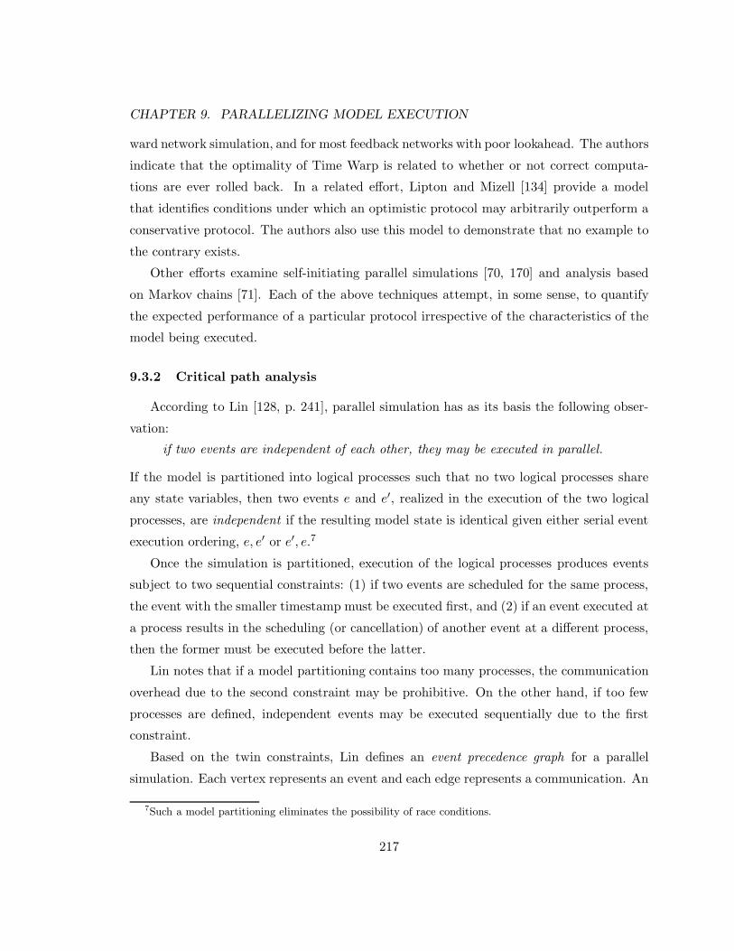
CHAPTER 9. PARALLELIZING MODEL EXECUTION
ward network simulation, and for most feedback networks with poor lookahead. The authors
indicate that the optimality of Time Warp is related to whether or not correct computa-
tions are ever rolled back. In a related effort, Lipton and Mizell [134] provide a model
that identifies conditions under which an optimistic protocol may arbitrarily outperform a
conservative protocol. The authors also use this model to demonstrate that no example to
the contrary exists.
Other efforts examine self-initiating parallel simulations [70, 170] and analysis based
on Markov chains [71]. Each of the above techniques attempt, in some sense, to quantify
the expected performance of a particular protocol irrespective of the characteristics of the
model being executed.
9.3.2 Critical path analysis
According to Lin [128, p. 241], parallel simulation has as its basis the following obser-
vation:
if two events are independent of each other, they may be executed in parallel.
If the model is partitioned into logical processes such that no two logical processes share
any state variables, then two events e and e′, realized in the execution of the two logical
processes, are independent if the resulting model state is identical given either serial event
execution ordering, e, e′ or e′, e.7
Once the simulation is partitioned, execution of the logical processes produces events
subject to two sequential constraints: (1) if two events are scheduled for the same process,
the event with the smaller timestamp must be executed first, and (2) if an event executed at
a process results in the scheduling (or cancellation) of another event at a different process,
then the former must be executed before the latter.
Lin notes that if a model partitioning contains too many processes, the communication
overhead due to the second constraint may be prohibitive. On the other hand, if too few
processes are defined, independent events may be executed sequentially due to the first
constraint.
Based on the twin constraints, Lin defines an event precedence graph for a parallel
simulation. Each vertex represents an event and each edge represents a communication. An
7Such a model partitioning eliminates the possibility of race conditions.
217

CHAPTER 9. PARALLELIZING MODEL EXECUTION
event execution time is associated with each vertex. A communication delay is associated
with each edge. Since the event precedence graph is acyclic, a maximal weighted path can
be found. This path is called the critical path, and its cost is the minimal time required to
finish the execution of the parallel simulation.
The cost of the graph may be derived as follows.8 Let ge be an event such that event e
is scheduled due to the execution of event ge. If ge is not defined for an event e, then e is
prescheduled. Let pe be an event such that both events e and pe are scheduled for the same
process, and the execution of pe is followed by the execution of e. Let τ(e) be the earliest
time when execution of e starts. Let η(e) be the execution time of e. Let τ(e) be the earliest
time when execution of e completes. If every process is executed by a dedicated processor,
then,
τ(e) = τ(e) + η(e) (9.2)
Let δ(e) be the time to schedule event e. If ge and e are scheduled at different processes,
then δ(e) represents the message-sending delay. Otherwise, Lin assumes δ(e) is zero. This
gives,
τ(e) =
0 if neither ge nor pe exist,
τ(pe) if ge does not exist,
τ(ge) + δ(e) if pe does not exist,
max[τ(pe), τ(ge) + δ(e)] otherwise.
(9.3)
Finally, the cost for the critical path, Tp, and the sequential execution time, Ts are given
by,
Tp = max∀e
τ(e), and Ts =∑∀e
η(e) (9.4)
The optimal parallel simulation time is computed based on Equation (9.3). However,
the equation is only adequate for the case where every process is executed on a dedicated
processor. If the number of processors, P , is less than the number of processes, N , then
Tp is also affected by process assignment and process scheduling. Lin [128] considers only
static process assignment, but investigates three process scheduling policies: (1) all events
at a processor are executed in nondecreasing timestamp order, (2) among the events (of
different processes) available for execution at a processor, the event with the earliest arrival
8Note that in this development, time refers to wall clock (or real) time, as opposed to simulation time.
218

CHAPTER 9. PARALLELIZING MODEL EXECUTION
time is selected, and (3) among the events available for execution at a processor, the event
with the smallest timestamp is selected.
Several approaches to critical path analysis have been proposed. Lin couples the critical
path analyzer to a generic sequential simulator. Berry and Jefferson [30] instrument a
sequential simulation and take a trace of the events executed. The trace is then transformed
into an event precedence graph. Finally, the cost of the critical path is computed from the
graph. Livny [135] integrates a critical path analyzer with the DISS simulation. No event
trace is required, and graph construction is implicit. Both Berry and Jefferson and Livny
limit the case to P = N. Som et al. [220] describe a method based on analyzing events in a
constrained execution graph. This method does not require a logical process decomposition
of the model, although a corresponding model execution environment is not described.
Finally, some observations due to Lin [128]: (1) A large number of events must be
processed in critical path analysis before a reliable speedup prediction can be obtained.
Transient events should not be considered part of the total if the simulation is intended to
produce steady state results. (2) The number of processors for parallel simulation must be
selected to balance the effects of the twin constraints in order to yield maximal speedup,
and (3) When communication cost is much higher than event execution cost (e.g. 20 : 1),
the amount of speedup may be very low. In this case, adding processors has no benefit.
9.4 Parallel Direct Execution of Action Clusters
Overstreet [178] demonstrates that a CS can be converted into an equivalent specification
reflecting a process view. Conceivably this specification could be adapted to reflect a logical
process view and thereby utilize the extant PDES techniques and protocols. Such integra-
tion with existing approaches requires: (1) selecting an implementation environment, and
(2) describing a suitable translation scheme. Defining a general translation scheme appears
to be difficult and deserving of investigation. Another, perhaps more interesting, question is
that given the ACIG-based model of computation described in Chapter 8, what parallelism
can be identified and can it be effectively exploited? This question is investigated here.
The focus of this development is contrasted with traditional PDES in the following manner.
Within PDES the focus is singular: speed; that is, given a discrete event simulation model
(program) and a particular parallel machine, make the program run as fast as possible.
219

CHAPTER 9. PARALLELIZING MODEL EXECUTION
Thus, the techniques of PDES center on perturbations of the model (program) such that
processor utilization is maximized. The approach taken in this effort adopts a somewhat
different focus: specifically, can the parallelism available in a given model representation
(the ACIG) be exploited without additional burden being placed on a modeler?
In a DEAC simulation, action clusters define the “level of granularity.” A logical starting
point in a search for parallelism within a DEAC simulation is therefore at the level of
action clusters. The action cluster incidence graph does not naturally partition the state
space of the model; therefore expectations regarding asynchronous algorithms – to exploit
inherent activity parallelism – should perhaps be limited. This issue is addressed in greater
detail subsequently. If the exploitation of inherent event parallelism is considered, intuition
provides that such parallelism exists in the cascade of CACs that accompanies each DAC.
In order to focus the development of concepts, for the remainder of this chapter we assume
that the transition specification is comprised entirely of ACs, i.e. the use of functions is not
considered.
9.4.1 ACIG expansion
Since action clusters provide the level of granularity, and the basis for parallelism, the
requirements of an implementation favor as many ACs as possible. More ACs means more
potential parallelism. The opposite is often true, however, at the specification level. For
a model specification in the CS, fewer ACs generally equates to a more understandable
communicative model.
For example, consider the MVS model in Chapter 6. If a large number of CPUs are
defined, a modeler is likely to describe the model (under the CM/CS approach) using
indexed objects. As a result, a single action cluster for begin-service might be defined as
follows:
for all i : 1 ≤ i ≤ N :: Cpu[i].status = idle and not empty(CpuQ[i]):Cpu[i].status := busyset alarm(Cpu[i].end service, exp(Cpu[i].service mean))
If a begin-service may occur during the same instant for multiple CPUs, clearly these actions
are independent and may be processed in parallel. Thus, whenever a model specification
includes quantified ACs such as the one given above, during the creation of the model
220

CHAPTER 9. PARALLELIZING MODEL EXECUTION
implementation, a translator (perhaps with assistance required from the modeler) may
expand the specification thereby affording an the capability to execute these ACs in parallel
on separate processors. The ACIG corresponding to this specification is referred to as the
expanded ACIG.9 Although the two forms are closely related, an important distinction must
be made: the ACIG is part of a model specification, the expanded ACIG provides a basis
for a model implementation.
9.4.2 A synchronous model for parallel execution
In this section, a pedagogical model for a synchronous parallel execution of an ACIG
on a hypothetical machine is described. The goal of this development is to enhance the
reader’s insight into the nature of the inherent event parallelism within an ACIG.
Let M be a model specification in the CS and let G be a simplified, expanded ACIG for
M. In a manner similar to Petri nets (see Chapter 4) we define a marking on the ACIG as
the distribution of tokens within the graph. Assume the existence of a hypothetical machine
capable of executing an ACIG. Graph execution is governed by the following rules:
• Whenever a token is passed to an AC, the condition is tested. If the condition evaluatesto false, the token is consumed. Otherwise, the actions are executed, a token is createdand passed to each of the state-based successors of the AC, and the token originallypassed to the AC is consumed.
• Whenever the situation develops that no tokens exist in the graph, the earliest sched-uled alarm (and all those with identical alarm times) is (are) removed from a list ofscheduled alarms, and a token is passed to each of the corresponding AC(s).
Execution begins by passing a token to the initialization AC and ends when the actions of
the termination AC are executed.
If an omniscience is permitted such that the ACIG and its markings are visible during
execution, what we observe is a static graph within which tokens flow sporadically: a token
appears in the initialization AC, is consumed, and tokens flow to its state-based successors.
Tokens continue to flow through the graph and are consumed and others created to take
their place until the last token reaches a “dead end” on its path from the initialization AC.
This occurs when the condition on the AC failed or no state-based path out of the AC
9The concept of ACIG expansion appears closely related to the common multiprocessor technique of“loop unrolling” (see [224, Chap. 7]).
221

CHAPTER 9. PARALLELIZING MODEL EXECUTION
exists. Then a brief pause – discernible only to the truly omniscient – and a token appears
at a DAC somewhere in the graph. Then, another cascade of tokens flowing, and so on.
From this vantage, the parallelism is visible. Namely,
the available parallelism at any point in (real) time is defined by the number oftokens in existence in the graph at that time.
Of course, this model describes an ideal situation that cannot exist in actual practice. In
the following sections, some limitations on this ideal are quantified.
9.4.3 Specification ambiguity
In Chapter 5, Overstreet’s characterization of specification ambiguity is given. Over-
street defines two types of ambiguity: state ambiguity and time ambiguity. State ambiguity
relates to a dependency among simultaneously enabled contingent action clusters, and time
ambiguity relates to a dependency among simultaneously enabled determined action clus-
ters. He further shows that detecting either state ambiguity or time ambiguity cannot be
accomplished automatically for an arbitrary model specification.
To provide consistency with the DEAC model of computation defined in Chapter 8,
and to establish a basis for denoting that the parallel execution of two action clusters
is well-defined, Overstreet’s definitions for ambiguity are modified slightly here. First, a
characterization of dependency among two model actions (in a CS) must be given.
Definition 9.3 Two model actions a and b are said to be write/write conflicting if theintersection of their output attribute sets is non-empty.
Definition 9.4 Two model actions a and b are said to be read/write conflicting if theintersection of the input and control attribute sets of one and the output attribute set ofthe other is non-empty.
Definition 9.5 Two model actions a and b are said to be dependent if they are write/writeor read/write conflicting. Otherwise a and b are independent.
The characterization of dependency given by Definition 9.5 is stronger than the definition
typically used in PDES.10 The PDES requirement of a totally partitioned state space makes
10As presented in Section 9.3.2, two events are independent if any serial ordering of their execution yieldsthe same state.
222

CHAPTER 9. PARALLELIZING MODEL EXECUTION
Event 1 Event 2
1 2
3 4 5
6 7
8
Figure 9.5: A Partial ACIG Showing Two Events with Common Actions.
considerations for processor contention unnecessary. However, in a parallel execution based
on an ACIG, the possibility exists for contention on model attributes.
For the following definitions, the relationship between action clusters in an ACIG and
action clusters corresponding to an event must be provided. At first glance it may appear
that to delineate the events in an ACIG, merely removing the dashed arcs is sufficient.
The remaining connected components should contain the events. This approach is almost
correct, but must be adapted slightly. Consider the ACIG fragment given in Figure 9.5.
The figure illustrates two events which share CACs. This type of specification often results
whenever a series of common actions occurs over several model events. For example, a
group of actions representing get-proper-signatures may occur both for the event that an
order is placed for spare parts, and the the event that a seaman is transferred.
To identify events in an (simplified) ACIG, a collection of graphs is constructed each
of which consists of a single DAC and all CACs reachable from it without passing through
another DAC. Algorithms for this are straightforward and may be found in [178, 194].
Definition 9.6 Let M be a model specification in the CS and let G = ACIG(M). LetE be the graph induced from G by a single DAC and all CACs reachable from it withoutpassing through another DAC. We call E an event-cluster.
Using these event-clusters as a basis, the ambiguity problem reduces to an examination of
conflicts within an event-cluster and among pairs of event-clusters.
223

CHAPTER 9. PARALLELIZING MODEL EXECUTION
Definition 9.7 Let M be a model specification in the CS, and let a and b be dependentmodel actions. If a and b are in distinct CACs of the same event-cluster, E, and if noordering information is available relative to a and b, then M is said to be state ambiguous.
Definition 9.8 Let M be a model specification in the CS, and let a and b be dependentmodel actions. If a and b are in ACs of distinct event-clusters, E1 and E2, and if no orderinginformation is available relative to a and b, then M is said to be time ambiguous.
Essentially, ambiguity can arise from two sources. First, ambiguity may be the result of
a poorly defined event. That is, within the cascade of CACs that accompanies a DAC
some dependency exists on attributes of two ACs whose respective order of execution is not
prescribed. This is state ambiguity as given by Definition 9.7. Time ambiguity, as given by
Definition 9.8, arises as the result of simultaneous (interfering) events.
The fundamental limitation confronting the automated detection of ambiguity is an
inability to statically determine read/write and write/write conflicts. Still, an ACIG may
posses certain properties which tend to indicate the presence of, or at least the possibility
for, ambiguity. We now describe a necessary condition for state ambiguity in a CS. The
Theorem clarifies the nature of the “ordering information” referred to in Definition 9.7. Let,
M = a CS model specification comprised of action clusters (AC1, . . . , ACn)O(ACj) = the set of output attributes for ACjI(ACj) = the set of input and control attributes for ACjWW ≡ ∃ i, j O(ACi) ∩O(ACj) = ∅RW ≡ ∃ i, j (O(ACi) ∩ I(ACj) = ∅) ∨ (I(ACi) ∩O(ACj) = ∅)G = simplified, expanded ACIGE = the set of event-clusters in G
Theorem 9.1 Let M be a model specification in the CS. If M is state ambiguous then∃ e ∈ E for the DAC d ∈ e, and two CACs i, j ∈ e, RW or WW holds for i, j and eitherno directed path between i and j exists or multiple paths from d to either i or j exist.
Proof: Let M be a model specification in the CS such that M is stateambiguous. Then by definition, there exists e ∈ E and CACs i, j ∈e RW or WW holds.Let d ∈ e be the DAC. By the construction of e, ∀ x ∈ e ∃ a directedpath from d to x. Let Pi denote the path from d to i. Let pj denotethe path from d to j.
Suppose pi is the unique path in e from d to i, and pj is the uniquepath in e from d to j. Further, suppose that a directed path, p∗,between i and j exists. Without loss of generality, suppose p∗ is apath from i to j.
224

CHAPTER 9. PARALLELIZING MODEL EXECUTION
1
2
3
4
Figure 9.6: A Partial ACIG Showing Multiple Paths Between a DAC and CAC.
Let M ′ be an implementation of M under the DEAC algorithm. Lett be any instant of M ′ during which i and j occur. Then i and jmust be coincident in time with d. Further, d must precede both iand j. Therefore, during instant t execution begins at d and followsthe path pi to i and pj to j. Since pj is the unique path from d to j, p∗must lie on pj. Otherwise, the concatenation of paths pi and p∗ forma directed path from d to j distinct from pj. Therefore, executionmust begin with d, follow pi to i and then follow p∗ to j.This contradicts the fact that M is state ambiguous since an explicitordering between i and j exists. Therefore the supposition must befalse and either multiple paths exist in e from d to one of i or j, orno directed path exits in e between i and j. 2
The proof of Theorem 9.1 is complicated by the fact that the members of E are not
required to be rooted trees, i.e. cycles in the underlying graph are possible. For example,
an event-cluster of the form illustrated in Figure 9.6 is permitted. This figure illustrates a
significant ambiguity problem with the ACIG itself. Specifically, when an AC has multiple
incoming arcs, e.g. AC4, the graph itself does not contain sufficient information to indicate
the conditions under which that AC may actually be enabled during an execution of the CS.
Is the information passed along one arc sufficient to enable the execution of the AC or must
information arrive at the AC from all incoming arcs? In the case of Figure 9.6, if either of
AC1 or AC3 can enable the execution of AC4, then the specification is potentially ambiguous
– if AC2 or AC3 conflicts with AC4. Otherwise, if both AC1 and AC3 must execute prior
to the execution of AC4 for any given instant, the specification is not ambiguous.
A necessary condition for time ambiguity is trivial, and little can be gleaned from the
225

CHAPTER 9. PARALLELIZING MODEL EXECUTION
graph structure. Essentially, if a CS is time ambiguous, some pair of event-clusters contains
conflicting actions. To resolve time ambiguity, a model analyzer must scan pairs of event-
clusters for conflicts – not guaranteed a priori determinable – and rely on the modeler’s
understanding to determine if the two events can occur during the same instant.
9.4.4 Critical path analysis for PDEAC simulation
Characterizations of inherent parallelism are formulated in Section 9.2. The position is
advanced that inherent parallelism should be regarded as a function of the model represen-
tation and not the underlying system. This point is worthy of elaboration. To be precise,
the available parallelism in a model is relative to the degree of dependence among model
components – for some given definition of dependence and some level of component, e.g.
event, activity, action. The dependence might reflect a dependence in the system, or it can
be an artifact of the model itself. Since the number of possible models for any given system
and set of objectives is likely to be very large, demonstrating that some dependency in the
system must be reflected in any model of that system is typically impractical. Hence, the
adoption of the position that inherent parallelism should be considered a property of the
model representation.
In Section 9.4.2 a model of the synchronous parallel execution of an ACIG is described.
In this section, a technique to establish the optimal parallel simulation time based on the
synchronous model of execution is defined. Such an assessment is desirable in order to
evaluate “how well” an actual PDEAC algorithm is performing, not relative to an artificial
constraint such as the maximum utilization of available processors, but relative to the
natural limitation of the available parallelism in a given model representation.
Lin [128] shows that a critical path analyzer can be incorporated into a sequential sim-
ulator. While this approach is less than ideal in many PDES settings – it requires the
development of both a sequential and a parallel model (program) – such an approach is
perfectly suited for the CM/CS development described by this research since the same
model specification may be used as the basis for both the sequential and the parallel imple-
mentation.
226

CHAPTER 9. PARALLELIZING MODEL EXECUTION
9.4.4.1 The synchronous critical path
Using the synchronous model for execution described in Section 9.4.2, the critical path
in a direct execution of action clusters simulation may be defined as follows.11 Based on
Lin’s development, let,
a = an action clusterpa = the action cluster that precedes a (from ACIG) if a is a CACαa = the set of ACs executed during the instant immediately
preceding the instant during which a executesτ(a) = the earliest time when execution of a may beginζ(a) = the time required to test the condition of aη(a) = the time required to perform the actions of aτ(a) = the earliest time when execution of a may complete
If every AC is executed by a dedicated processor, then,
τ(a) = τ(a) + θ(a) (9.5)
Where θ(a) = ζ(a) + η(a) if the condition on a is true, and θ(a) = ζ(a) otherwise. The
earliest time when the execution of a may begin is given by,
τ(a) =
0 if a is the initialization AC,
τ(pa) if pa exists,
max∀x∈αa τ(x) otherwise.
(9.6)
Finally, the cost for the critical path, Tp, and the sequential execution time, Ts are,
Tp = τ(t), and Ts =∑∀a
η(a) (9.7)
where t denotes the termination AC. The optimal parallel simulation time of any syn-
chronous PDEAC algorithm for a given model is Tp, with a best possible speedup of TsTp.
9.4.4.2 The critical path algorithm
An algorithm to compute the (synchronous) critical path of a DEAC simulation is given
in Figure 9.7. The algorithm is simply an augmentation of the standard DEAC algorithm
(Figure 8.4). Initially, τ(pa) is set to zero for all CACs, a, in the CS. Whenever an AC is
11Recall from Chapter 8 that execution of an AC is defined as the evaluation of the condition on the AC,followed by activation of the AC – performing the specified actions – if the condition evaluates to true.
227

CHAPTER 9. PARALLELIZING MODEL EXECUTION
LetA be the ordered set of scheduled alarms.
Let C be the set of state-based clusters whose conditions should be tested immediately.Let σiS be the set of state-based successors for action cluster σi (where 1 ≤ i ≤ | ACs | ).
Initially
1 ∀σi, set σiS (from simplified ACIG);A = C = ∅; ∀ CACs j, τ(pj)← 02 perform actions of initialization AC, σI3 τ(σI)← η(σI); max← τ(σI); ∀ j ∈ σIS , τ(pj)← τ(σI)4 add σIS to C
5 while (C = ∅)
6 remove σa ← FIRST(C)7 τ(σa) ← τ(pσa) + ζ(σa)8 if condition on σa is true
9 perform actions of σa10 τ(σa)← τ(σa) + η(σa); ∀ j ∈ σaS , τ(pj) ← τ(σa)11 add σaS to C12 endif
13 if τ(σa) > max, max← τ(σa)14 endwhile
Simulate
15 while (true) do
16 clock← time given by FIRST(A)
17 α←max
18 while (clock = time given by FIRST(A)) do
19 remove FIRST(A); let σa be the AC corresponding to FIRST(A)20 perform actions of σa21 τ(σa)← α + η(σa); emax← τ(σa); ∀ j ∈ σaS , τ(pj)← τ(σa); add σaS to C22 while (C = ∅)
23 remove σa ← FIRST(C)
24 τ(σa)← τ(pσa) + ζ(σa)25 if condition on σa is true
26 perform actions of σa27 τ(σa)← τ(σa) + η(σa); ∀ j ∈ σaS , τ(pj)← τ(σa)28 add σaS to C29 endif30 if τ(σa) > emax, emax← τ(σa)31 endwhile
32 if emax > max, max← emax
33 endwhile
34 endwhile
Figure 9.7: The Critical Path Algorithm for a DEAC Simulation.
228

CHAPTER 9. PARALLELIZING MODEL EXECUTION
invoked: (1) its completion time is recorded as the completion time of its predecessor plus
the execution time of the AC itself,12 and (2) if the actions given by a are taken, for all ACs
i in the successor set of a, the completion time of a is recorded as the completion time of
the predecessor of i. In the simulation proper (lines 15 - 34), three variables are utilized to
track the critical path: max contains the largest value of τ for each instant, emax contains
the largest value of τ for each event-cluster, and α contains the largest value of τ for the
previous instant. We now formally establish the correctness of the critical path algorithm.
Lemma 9.1 In the critical path algorithm, whenever the clock is updated (line 16), maxcontains the maximum value of τ(a) for all ACs a executed during the previous instant.
Proof: Execution of a model under the DEAC algorithm may be viewed asa sequence of instants, I1, I2, . . . Im. We proceed by induction onj : 1 ≤ j ≤ m.
Basis. j = 1. Under the CM, initialization is not considered an in-stant. Model execution begins with the first update to the systemclock (line 16). Therefore, in the critical path algorithm, the begin-ning of the jth instant is defined by the jth execution of line 16.Consider j = 1. The body of the simulation proper (the while loop ofline 15) has not executed. Therefore the value of max is determinedin the initially section of the algorithm (lines 1 - 14). We see thatmax is first assigned to the earliest possible completion time of theinitialization AC at line 3. If initialization has no state-based suc-cessors, the assignment to max is correct and the hypothesis holds.If initialization has state-based successors, the loop of line 5 is ex-ecuted. In all cases (i.e. whether or not the condition on the ACevaluates to true) max is updated correctly (line 13). Therefore thehypothesis holds for j = 1.Inductive step. Assume that the hypothesis holds for j ≤ n for somen ≥ 1. We show that it also holds for j = n+ 1.The jth instant begins with the jth execution of line 16. Considerthe j − 1st execution of line 16. By the inductive hypothesis, maxcontains the maximum value of τ(a) for all ACs a executed duringthe preceding (j−2nd) instant (or initialization, if the j−2nd instantdoes not exist). This value is placed in α by the j− 1st execution ofline 17.The completion time of the DAC defining the j − 1st instant is cal-culated at line 21 as τ(σa) ← α + η(σa) and this value is stored inthe variable emax.
12The completion time of the predecessor of AC i is given by τ(pi) if i is a CAC, or by α if i is a DAC.
229

CHAPTER 9. PARALLELIZING MODEL EXECUTION
If the DAC has no state-based successors, the while loop given byline 22 is not iterated. Otherwise emax is updated for each CAC,if necessary, such that emax contains the largest value of τ for thatevent-cluster (line 30).In either case, max is assigned the final value of emax at line 32.If no other DAC occurs during instant j − 1, then the while loopgiven by line 18 terminates and the hypothesis holds.If another DAC occurs during instant j−1, then the earliest comple-tion time of that DAC is calculated correctly using α (line 21) andthis value is assigned to emax. As before, the while loop given byline 22 is iterated for any CACs as necessary and emax is correctlyupdated at line 30.After all ACs defining the event-cluster have executed, max is up-dated, if necessary, at line 32. If another DAC occurs during instantj − 1, this process repeats. Otherwise the while loop terminates andthe hypothesis holds. 2
Lemma 9.2 In the critical path algorithm, following the execution of an AC, a, τ(a) con-tains the earliest possible finishing time of a.
Proof: Execution of a model under the DEAC algorithm may be viewed asa sequence of ACs, AC1, AC2, . . .ACm. We proceed by induction onj : 1 ≤ j ≤ m.
Basis. j = 1. The first AC executed in the critical path algorithm isthe initialization AC, i. Immediately following the execution of i, τ(i)is computed as τ(i) ← η(i) (line 3). If execution begins at time 0,then i may complete no earlier than η(i). Therefore the hypothesisholds for j = 1.Inductive step. Assume that the hypothesis holds for j ≤ n for somen ≥ 1. We show that it also holds for j = n+ 1.Case I. j is a DAC. Immediately following the execution of j, τ(j) iscomputed as τ(j) ← α + η(j) (line 21). By Lemma 9.1, α containsthe maximum value of τ(a) for any AC a executed during the pre-ceding instant. Therefore τ(j) is assigned the correct value and thehypothesis holds.Case II. j is a CAC. Immediately prior to the evaluation of thecondition on j, τ(j) is assigned the value of τ (pj)+ζ(j) (lines 7, 24).Let l be the index of pj . l ≤ n. Therefore, by the inductive hypothesis,τ(pj) is the earliest possible finishing time for pj. So τ(j) contains theearliest possible completion time for the evaluation of the conditionon j and if the condition evaluates to false, the hypothesis holds.If the condition on j evaluates to true, τ(j) is incremented by η(j)(lines 10, 27). In this case, τ(j) contains the earliest possible com-pletion time for the evaluation and activation of j, and therefore thehypothesis holds. 2
230

CHAPTER 9. PARALLELIZING MODEL EXECUTION
Theorem 9.2 If the critical path algorithm terminates, τ(termination) contains the costof the critical path.
Proof: Lemma 9.2 establishes that following the execution of any AC a, τ(a)contains the earliest possible finishing time for AC a.
Therefore if the termination AC, t, appears in the sequence of ACsproduced by an execution of the critical path algorithm, τ(t) containsthe earliest possible finishing time of the termination AC. This valuedefines the earliest possible completion time for the model, which isdefined to be the cost of the critical path. 2
Note that τ(termination) may not be equal to max τ(a), for all ACs a in the execution
sequence, since some ACs may be coincident with termination such that the execution time
of one or more of these ACs is greater than the execution time of the termination AC.
However, the semantics of a DEAC simulation are such that termination during an instant
supersedes any attribute value changes that occur during that instant. Therefore, in a
typical model, if n CACs, one of which is the termination AC, are coincident with a DAC,
d, then a directed path from each of the remaining n−1 CACs to the termination AC exists
in the ACIG. In this case, and in the case where termination is a DAC, τ(termination) =
max τ(a) for all ACs a in the execution sequence.
9.4.5 PDEAC algorithm
In this section, an algorithm for a parallel direct execution of action clusters (PDEAC)
simulation is described. The algorithm reflects the synchronous model of computation
described in Section 9.4.2. Recall that the model of computation maintains the AC as the
element of interest. Thus, the algorithm described here equates AC and process. In an ideal
situation, each AC would be executed on a dedicated processor. This situation is assumed
in the critical path calculations (Section 9.4.4.2). Note that in such a configuration, a
maximum utilization of available processors would not be achieved. But such is not the aim
of this approach. The goal here is that a model implementation produce an execution time
as close as possible to that of the critical path.
For a typical model, the number of ACs is probably much greater than the number of
available processors. As a result, processor mapping and load balancing become issues of
concern if the critical path time is to be approached. Several methods for dealing with these
231

CHAPTER 9. PARALLELIZING MODEL EXECUTION
while true do
passivate
if condition on AC is trueperform actions
activate state-based successors
end while
Figure 9.8: An AC Process in the PDEAC Algorithm.
issues are evident:
• A static assignment of ACs to processors. This approach incurs the least overheadrelative to the underlying computation. Static analysis methods such as the principalcomponents and factor analysis techniques suggested by [26, 27, 145] could be adaptedto map ACs to processors such that the likelihood that any two ACs on the sameprocessor could be simultaneously eligible for execution is minimized. However, thelimitations of such static analysis follow from Overstreet’s Turing evaluation of theCS [178, Ch. 8].
• An assignment of ACs to processors with migration under dynamic load balancing.The limitations of static process mapping have been noted within PDES, and dynamictechniques are currently the subject of intensive research effort (see [171]). As thesetechniques mature, they should be readily adaptable within the CM/CS approach.
• Dynamic process scheduling. A central (or perhaps distributed) process schedulercould be utilized such that during clock update the scheduler assigns ACs to proces-sors. The list of ACs eligible for execution during an instant is derivable from thestate of the alarm list and from the event-clusters as given by the ACIG.
In the PDEAC algorithm, the behavior of an AC may be described as given by Figure 9.8.
The figure presents logic suitable for both CACs and DACs if the condition on a DAC is
defined as a tautology. Upon activation, an AC evaluates its condition. If the condition is
true, the actions given by the AC are performed and the state-based successors of the AC
are activated. Initialization and time flow within the algorithm are governed by a manager
process as depicted in Figure 9.9.
The manager activates the initialization AC and then enters the simulation proper. After
all ACs during an instant (or initialization) have finished executing, the manager updates
the clock based on the alarm list, and activates the DAC(s) whose alarm time(s) is (are)
equal to the current clock value.
232

CHAPTER 9. PARALLELIZING MODEL EXECUTION
activate the initialization AC
while true do
when no ACs can executeupdate clock
activate DAC(s) with current clock
end while
Figure 9.9: The Manager Process in the PDEAC Algorithm.
The primary technical issue to resolve in this algorithm is the detection of when the
clock may be safely updated. In the model of computation described in Section 9.4.2, when
the last AC for a given instant consumes its token, the DAC(s) defining the next instant are
“magically” (via omniscience) passed tokens. Implementing this exchange, however, requires
global knowledge in a distributed environment – an historically challenging problem.
A simple solution is for each AC to send the list of ACs it activates to the manager,
and for each AC to notify the manager upon its own completion. Such an approach may
likely produce a bottleneck within the computation. Alternatives may be to distribute the
manager process itself, or exploit the facilities of a given architecture or thread package.
We leave these important details for future research.
9.4.6 Unresolved issues
The efforts of this chapter represent the first small steps toward effective mechanisms
for the parallel execution of simulation models within a CM/CS development framework.
The goal of this chapter is to establish the definitional and methodological basis which must
underly any execution environment. The concept of inherent parallelism and its relationship
to an action-cluster-based simulation is crucial in this regard, and is established here. Fur-
ther, an algorithm with which to estimate the inherent parallelism in a CS representation
is defined and its correctness formally established.
These efforts make a significant contribution to the theoretical basis for exploiting par-
allelism within the CM/CS framework, but much work remains to be completed in the
practical application of the theory. Perhaps the best way to proceed from here is to es-
tablish an experimental environment within which the practical ideas and methods from
233

CHAPTER 9. PARALLELIZING MODEL EXECUTION
PDES research may be applied and resolved with the context and theories of the CM/CS
approach. To this end, several issues of substance need to be addressed:
• Contention on the alarm list. The PDEAC approach does not partition the statespace among the available processors. Therefore contention on shared variables mustbe explicitly handled. However, given a CS model representation that contains nostate or time ambiguities, the only contention caused by actions of ACs executing inparallel occurs at the alarm list. To prevent the scheduling of alarms from becominga bottleneck, mechanisms exploiting the “event horizon” concept may prove useful(see [221, 222]).
• Action-level parallelism. The efforts described here have only considered parallelismat the level of the action cluster. Each action cluster is regarded as a small sequentialalgorithm. The actions within an AC may exhibit a degree of independence and maypermit the definition, and exploitation, of “finer grains” of parallelism.
• Handling functions. In the development of Chapters 8 and 9, a CS is assumed to becomprised solely of ACs. Allowing functions to be utilized in the specification of modelbehavior leads to many questions regarding analyzability and also implementability.One possible solution is to define techniques by which functions may be translatedinto ACs.
• Asynchronous execution. The models and algorithms described in this chapter are syn-chronous in nature – dealing with inherent event parallelism as defined in Section 9.2.1.Adapting extant asynchronous techniques from PDES, e.g. optimism, for use withinthe CM/CS approach merits investigation. Such efforts, however, require reconcilingthe ACIG representation with the requirements of a partitioned state space.
Clearly, the CM/CS approach requires much further investigation in this area. Just as clear,
hopefully, is that the CM/CS approach has much offer.
9.5 Summary
The execution of discrete event simulation programs using multiple processors is inves-
tigated in this chapter. Parallel discrete event simulation is evaluated from the modeling
methodological perspective identified in Chapter 3. Differences are noted and recommenda-
tions made to reconcile these two disparate views. The capabilities of the CM/CS approach
relative to parallel execution are also investigated. The concept of inherent parallelism is
described. Inherent parallelism is a function of a given model representation and estab-
lishes a bound on the expectations for speedup resulting from the application of multiple
processors to an implementation of the model.
234

CHAPTER 9. PARALLELIZING MODEL EXECUTION
A synchronous model of execution is defined for the CS, and a parallel direct execution
of action clusters (PDEAC) algorithm – based on this model – is given. A critical path algo-
rithm, also based on the synchronous model, is defined as an augmentation of the standard
DEAC algorighm (see Chapter 8) such that inherent parallelism is readily quantifiable.
The concepts of state ambiguity and time ambiguity in a CS are refined, and a necessary
condition for state ambiguity is identified.
235

Chapter 10
CONCLUSIONS
“Oh, now, don’t underestimate the abacus,” said Reg. “Inskilled hands it’s a very sophisticated calculating device, fur-thermore it requires no power, can be made with any mate-rials you have to hand, and never goes bing in the middle ofan important piece of work.”
Douglas Adams, Dirk Gently’s Holistic Detective Agency
The proposition underlying this research is a basic one: discrete event simulation model
development must be guided by recognition of the fundamental role of decision support and
its relationship to model correctness. Motivating this effort is an observation that technol-
ogy, and not the principles of decision support, is exerting major influences on the course
of simulation research in many areas – parallel discrete event simulation and distributed
interactive simulation being two examples.
In Chapter 1, a set of objectives for this research is identified. The most basic objective
is described as seeking an answer to a central question of discrete event simulation modeling
methodology: what is the nature of the ideal framework for simulation model development
where the models may be used for a wide variety of purposes, and implemented on varying
architectures? Such an ambitious objective cannot be realistically achieved within the scope
of a Ph.D. dissertation. Still, its formulation is important because the objective represents
a target toward which the research described here must move. The map within which
the tasks comprising the research effort are charted is provided by a more focused set of
objectives:
1. Identify an extensible framework for model development which permits the integrationof emerging technologies and approaches, and demonstrate its feasibility using an
236

CHAPTER 10. CONCLUSIONS
existing methodology and representation form(s).
2. Recognize a potential problem with the focus of parallel discrete event simulationresearch, and demonstrate how the framework described above may be utilized to cost-effectively incorporate parallel execution within the general discrete event simulationparadigm.
An evaluation of this work with respect to the research objectives appears in Section 10.2.
Prefacing the evaluation is the summary of results and identification of research contribu-
tions presented in Section 10.1. Finally, in Section 10.3, some directions for future research
are described.
10.1 Summary
The most tangible contributions of this research result from developments with the Con-
dition Specification. This work represents the most intensive investigation of the language
since its development in 1982. Research contributions are made in many areas. However,
several contributions are solely in terms of the global objective – an objective not attainable
within the scope of this effort – and are therefore resistant to conclusive evaluation. In the
following sections, the research is summarized, and contributions noted, by chapter.
10.1.1 Discrete event simulation terminology
The terminological basis for this research is outlined in Chapter 2. Discrete event
simulation is distinguished from other types of simulation, and noted to be at the focus
of this effort. Definitions are provided for the ubiquitous terms system and model, and
Nance’s [156] characterization of the time and state relationships in a simulation model is
reviewed.
10.1.2 A philosophy of model development
Chapter 3 outlines a philosophy of simulation model development characterized as rep-
resentative of the “modeling methodological view” of discrete event simulation. The view
holds that the primary function of discrete event simulation involves decision support. The
presentation covers a broad range of topics including: (1) a delineation of the relationship
among life cycle, paradigm, methodology, method and task; (2) a review of the life-cycle
237

CHAPTER 10. CONCLUSIONS
model for a simulation study proposed by Balci and Nance; (3) a discussion of some im-
portant issues in model representation; and (4) a brief description of the simulation model
development environment (SMDE) project. The research contributions from Chapter 3 are
the following:
• Requirements for a next-generation modeling framework. In a 1977 report, Nance [153]identifies six criteria for a simulation model specification and documentation language.Sargent [205], in a 1992 conference paper, offers fourteen requirements for a modelingparadigm. These two sets of criteria are reconciled to produce a list of ten requirementsfor a next-generation modeling framework (see Table 3.1):
1. Encourages and facilitates the production of model and study documentation,particularly with regard to definitions, assumptions and objectives.
2. Permits model description to range from very high to very low level.3. Permits model fidelity to range from very high to very low level.4. Conceptual framework is unobtrusive, and/or support is provided for multiple
conceptual frameworks.5. Structures model development. Facilitates management of model description and
fidelity levels and choice of conceptual framework.6. Exhibits broad applicability.7. Model representation is independent of implementing language and architecture.8. Encourages automation and defines environment support.9. Support provided for broad array of model verification and validation techniques.
10. Facilitates component management and experiment design.
These requirements serve as the evaluative basis for the survey in Chapter 4.
• An abstraction based on a hierarchy of representations. The model developmentparadigm utilized within the SMDE is abstracted to accommodate multiple imple-mentations as illustrated in Figure 3.4. The abstraction identifies three levels ofmodel representation:
1. Modeler-generated specifications. These representational forms permit a modelerto describe system definitions, assumptions and the set of objectives for a givenstudy, as well as the model behavior in a manner suitable to meet the objectives.While a canonical form is implied by the figure, the nature of this form has notbeen defined.
2. Transformed Specifications. Adhering to the principle of successive refinement,automated and semi-automated transformations are defined to various forms thatenable analysis and translation to implementations meeting a specified criteria.
3. Implementations. The lowest level of the transformed specifications are theimplementations. These executable representations satisfy the particular con-straints of a given simulation study.
238

CHAPTER 10. CONCLUSIONS
The hierarchy may be envisaged as being composed of a set of cooperative and con-gruent narrow-spectrum languages, or as a single wide-spectrum language. In eitherapproach, the representation should be the focal point, and the subject of explicitmethodological support.
10.1.3 Formal approaches to discrete event simulation
In Chapter 4, a survey of formal approaches to discrete event simulation modeling is
presented. The research contributions from Chapter 4 are the following:
• Survey and evaluation of formalisms. Eight categories of formal methods are identifiedand surveyed. Each category is reviewed in terms of its underlying concepts, historicaldevelopment, and directions of current and future research. The categories surveyedare: (1) Calculus of Change, (2) systems theoretic approaches (DEVS, System EntityStructure), (3) activity cycle diagrams, (4) event-oriented graphical techniques (eventgraphs, simulation graphs), (5) Petri nets, (6) logic-based approaches, (7) control flowgraphs, and (8) generalized semi-Markov processes. The formalisms are evaluated withrespect to the requirements for a next-generation modeling framework identified inChapter 3. The evaluation procedure defines four levels of support for a requirement:(1) not recognized, (2) recognized, but not supported, (3) demonstrated, and (4)conclusively demonstrated. The evaluation summary is given in Table 4.8.The survey indicates that no existing approach fully satisfies the requirements for anext-generation modeling framework. Of the approaches considered, the systems the-oretic approaches rate highest, and generalized semi-Markov processes rate lowest.1The requirement for an “unobtrusive conceptual framework” is viewed as least sup-ported by the surveyed approaches, and is the area where the greatest strides can bemade.
10.1.4 Foundations
Nance’s Conical Methodology (CM) and Overstreet’s Condition Specification (CS),
which provide the basis for the majority of tasks comprising the research, are reviewed
in Chapter 5.
The Conical Methodology is a model development approach that is intended to provide
neither abstract nor concrete definitions of general systems. The CM adopts the view
that model development leads potentially to myriad evolutionary representations, but that
the mental perception is the initial representation for every model, and that assistance in
the area of mental perception, or conceptualization, is (should be) a critical aspect of any
1Note that the CM/CS, as evaluated in Chapter 5, receives the highest overall rating.
239

CHAPTER 10. CONCLUSIONS
modeling methodology. The CM identifies two processes in model development: (1) model
definition, during which a model is described in terms of objects and the attributes of those
objects, and (2) model specification, during which the attribute value changes are described.
The Condition Specification is a world-view-independent model representation designed
primarily to support analysis. The CS permits model behavior to be described in terms
of a set of conditions and a set of actions. An action may be paired with the condition
that causes it, forming a condition-action pair (CAP), or groups of actions with the same
condition may be formed into an action cluster (AC).
10.1.5 Model representation
The CS is most suited for the middle level of the hierarchy described in Chapter 3.
The extensions and modifications described in Chapters 6 through 9 are primarily directed
to widen the spectrum of the language, and thus provide support throughout the hierar-
chy. In Chapter 6, the CS provisions for model development, with respect to the CM, are
investigated. The research contributions from Chapter 6 are the following:
• Complete development of four models. To evaluate the pertinent model representa-tion concepts, a complete development of four models is accomplished using the CMand CS. These models are: (1) a multiple virtual storage batch computer system,(2) a traffic intersection, (3) a system of colliding rigid disks, and (4) the machineinterference problem.
• New operations for the CS. The collection of primitives for the CS is extended tosupport CM facilities for set definition. Operations defined are: insert, remove,
member, find and class.
• Redefinition of form for report specification. Overstreet does not prescribe a specificform for the report specification, but instead indicates how the interface between thereport specification and the transition specification might be formed using a programdesigned to compute statistics. A higher-level form for the report specification isdefined (see Figures 6.9 and 6.25).
• Definition of the concept of “augmented” object and transition specification. A transi-tion specification need not contain any information regarding the collection of statistics(as long as this information is captured in the report specification), however, if thetransition specification is to serve as a basis for a model implementation, then the ac-tions required to facilitate statistics gathering – either “on-the-fly” or via logs – mustbe incorporated into the transition specification. The concept of an “augmented” spec-ification is outlined whereby the object specification and transition specification maybe automatically transformed to include the objects, attributes and actions necessary
240

CHAPTER 10. CONCLUSIONS
to provide statistics gathering. This transformation occurs as part of the movementfrom specification to implementation.
• Definition of the concept of experiment specification. Similar to the need for an “aug-mented” specification to capture the statistics gathering aspects of model behavior,an experiment specification is proposed to capture details, e.g. the condition for thestart of steady state, necessary to produce an experimental model.
• Evaluation of object-based versus object-oriented. The object-oriented paradigm hasarguable advantages over traditional programming approaches for large systems (froma software engineering perspective). The question is asked: from the point of viewof discrete event simulation model development, is a strict object-oriented approachsuperior to the object-based perspective of the CM? The suggestion is that the veryconstrained notions of method, and communication by message passing, may leadto an unnatural description of systems. Thus, the less constraining object-basedperspective of the CM is viewed as superior in terms of discrete event simulationmodel development.
10.1.6 Model generation
In Chapter 7, the extant methods to provide automated assistance in the generation of
a CS are reviewed. The model generation and related issues within the SMDE are surveyed.
Based on the model development lessons of Chapter 6, new directions for CM/CS-based
model generators are described. These new directions include: (1) AC-oriented develop-
ment, and (2) graphical front ends.
10.1.7 Model analysis and execution
In Chapter 8, issues in model analysis and execution are investigated. The research
contributions from Chapter 8 are the following:
• A semantics for the CS. In order to provide support for model implementation, thesemantic rules for the CS are reformulated. The reformulation includes interpretationsfor: (1) CAP, (2) AC, and (3) sequence of ACs.
• Definition of direct execution of action cluster simulation. Based on a model of com-putation provided by the ACIG, an implementation structure referred to as a directexecution of action cluster (DEAC) simulation is defined. A DEAC simulation issimply an execution of an augmented CS transition specification.
• Definition of minimal-condition DEAC algorithms. Figures 8.3 and 8.4 present algo-rithms for DEAC simulations that are described as “minimal-condition.” Minimal-condition implies that given a completely simplified ACIG as a basis, and using thesemantics for a CS mentioned above, the number of state-based conditions evaluated
241

CHAPTER 10. CONCLUSIONS
upon the execution of any given AC is minimal. Two algorithms are defined. Fig-ure 8.3 illustrates the minimal-condition algorithm for a CS containing mixed ACs.Figure 8.4 illustrates the minimal-condition algorithm for a CS without mixed ACs.
• Evaluation of new CS syntax and semantics on provisions for model analysis. Sincethe primary purpose of the CS has been to facilitate model analysis, the new CSsyntax and semantics are evaluated with respect to the extant provisions for modelanalysis in the CS. The evaluation indicates that only one analysis technique, actioncluster completeness, is affected by the expanded spectrum of the CS.
• Evaluation of multi-valued alarms. A potential source of ambiguity is identified inthe possibility of having a multi-valued alarm with a corresponding after alarm
statement. Static analysis cannot guarantee the correct use of the after alarm
construct, therefore a caveat should be provided to modelers regarding their use.
• Evaluation of CS as time-flow-mechanism-independent. One of the original goals forthe CS is time-flow-mechanism-independence. The failure of the CS in this regardis demonstrated. The use of the alarm construct in a CS must reflect some view ofthe passage of time (although not necessarily the implementation of time flow). Wepostulate that this problem exists for any operational specification language.
10.1.8 Parallelizing model execution
In Chapter 9, some issues relating to discrete event simulation and parallel execution
are addressed. The research contributions from Chapter 9 are the following:
• Case study of parallel discrete event simulation. Parallel discrete event simulation(PDES) research is evaluated from the modeling methodological perspective identi-fied in Chapter 3. Differences are evident in two areas: (1) the enunciation of therelationship between simulation and decision support, and the guidance provided bythe life cycle in this context, and (2) the focus of the development effort. Four recom-mendations are made for PDES research to be reconciled with the “mainstream” ofDES: (1) return the focus of the development effort to the model, (2) formulate exam-ples with enunciation of simulation study objectives, (3) examine methods to extractspeedup in terms of the particular model development approach and envisaged modelpurpose, and (4) examine the relationship of speedup to software quality.
• Definitions for inherent parallelism. The concept of inherent parallelism is implicitin the majority of PDES approaches, but has found explicit formulation within thecritical path literature. A new characterization, based on the time and state relation-ships identified by Nance, is given. Two types of inherent parallelism are described:(1) inherent event parallelism, which relates to the independence of attribute valuechanges that occur during a given instant, and (2) inherent activity parallelism, whichrelates to the independence of attribute value changes that occur over all instants ofa given model execution.
• Definition of the concept of ACIG expansion. Since action clusters provide the basisfor parallelism, the requirements of an implementation favor as many ACs as possible.
242

CHAPTER 10. CONCLUSIONS
An increased number of ACs yields more potential parallelism. The opposite is oftentrue, however, at the specification level. For a model specification in the CS, fewerACs generally equates to a more understandable communicative model. Conditionsare described by which ACs with quantified conditions may be expanded into a setof ACs, thus producing an expanded ACIG, which provides the basis for a parallelimplementation.
• Synchronous model of execution. In a manner similar to Petri nets, we define a markingon the ACIG as the distribution of tokens within the graph. Graph execution isgoverned by the passing of tokens. Whenever a token is passed to an AC, the conditionon the AC is tested. If the condition evaluates to false, the token is consumed.Otherwise, the actions of the AC are executed, a token is created and passed to eachof the state-based successors of the AC, and the token originally passed to the ACis consumed. Whenever the situation develops that no tokens exist in the graph, theearliest scheduled alarm (and all those with identical alarm times) is (are) removedfrom the list of scheduled alarms, and a token is passed to the corresponding AC(s).Execution begins by passing a token to the initialization AC and ends when the actionsof the termination AC are executed. The available parallelism at any point in (real)time is defined by the number of tokens in existence in the graph at that time.
• Redefinition of time ambiguity and state ambiguity. Overstreet defines two types ofambiguity: state ambiguity and time ambiguity. State ambiguity relates to a depen-dency among simultaneously enabled contingent action clusters, and time ambiguityrelates to a dependency among simultaneously enabled determined action clusters.New definitions for these terms are developed. The development includes characteri-zations of two central elements: (1) action dependence, and (2) event-cluster. Stateambiguity is defined as the existence of dependent actions (and the absence of execu-tion ordering information) within a single event-cluster, and time ambiguity is definedas the existence of dependent actions among simultaneously enabled event-clusters.
• Formulation of a necessary condition for state ambiguity. The fundamental limitationconfronting the automated detection of ambiguity is an inability to statically deter-mine action dependencies. Still, an ACIG may posses certain properties which tendto indicate the presence of, or at least the possibility for, ambiguity. A necessary con-dition for state ambiguity in a CS is formulated. The condition establishes that if aCS is state ambiguous then two ACs exist such that they are in the same event-clusterand either no directed path (in the ACIG) exists between the two ACs, or multiplepaths (in the ACIG) exist from the DAC defining the event-cluster to one of the ACs.This condition is proved as Theorem 9.1.
• Definition of a critical path algorithm for PDEAC simulations. Based on Lin’s de-velopment, a critical path algorithm for parallel direct execution of action cluster(PDEAC) simulations is developed. The algorithm is an augmentation of the stan-dard DEAC algorithm (defined in Chapter 8) and computes the synchronous criticalpath for a given model representation. The algorithm is given in Figure 9.7, and itsproof of correctness established in Lemmas 9.1 and 9.2, and Theorem 9.2.
• Description of synchronous PDEAC algorithm. Based on the synchronous model ofexecution, a PDEAC algorithm is described (Figures 9.8 and 9.9). The algorithm is
243

CHAPTER 10. CONCLUSIONS
complete but does not dictate a mechanism for detecting when the clock should beupdated. A suggestion is made for such a mechanism, but we note that the efficiencyof the mechanism hinges largely on the choice of implementation architecture andlanguage.
10.2 Evaluation
The research is evaluated with respect to the focused objectives identified in Chapter 1.
Objective 1. Identify an extensible framework for model development whichpermits the integration of emerging technologies and approaches, and demon-strate its feasibility using an existing methodology and representation form(s).
A set of requirements for a next-generation modeling framework, and an abstraction based
on a hierarchy of representations is given in Chapter 3. The framework and abstraction are
extensible in their provisions for both wide-spectrum and narrow-spectrum approaches. New
technologies are accommodated, and their influence encapsulated, at the implementation
level of model representation.
The Conical Methodology appears suitable to underly a next-generation modeling frame-
work. Much of the research described in Chapters 6 through 9 widens the spectrum of the
CS to support all three levels of representation described by the abstraction. Although many
issues remain unresolved, the feasibility of the framework, abstraction, and the CM/CS ap-
proach have been demonstrated. The research involving the CM/CS approach is assessed
with respect to gains in terms of the requirements for a next-generation modeling framework.
Requirement 1. Encourages and facilitates the production of model and study documenta-tion, particularly with regard to definitions, assumptions and objectives.
A distinctive characteristic of the CM, the research makes no specific contribution inthis area.
Requirement 2. Permits model description to range from very high to very low level.
By defining primitives for set manipulation in the CS, higher level descriptions ofmodel behavior than previously possible may now be captured in the CS. For example,descriptions of queueing behavior are simplified with the CS extensions.
Requirement 3. Permits model fidelity to range from very high to very low level.
Characteristic of an object-based model development approach, the research makesno specific contribution in this area.
244

CHAPTER 10. CONCLUSIONS
Requirement 4. Conceptual framework is unobtrusive, and/or support is provided for mul-tiple conceptual frameworks.
Although the CS is conceptual-framework-independent, working directly at the CSlevel imposes a somewhat restrictive CF. Chapters 6 and 7 describe methods by whichmodels may be developed at high levels under a variety of CFs, and how such a modeldescription may be reflected in the CS.
Requirement 5. Structures model development. Facilitates management of model descrip-tion and fidelity levels and choice of conceptual framework.
An important attribute of a model generator, the research makes no specific contri-bution in this area.
Requirement 6. Exhibits broad applicability.
Through the complete development of the four disparate models in Chapter 6 – onlyone of which, the machine interference problem, having been previously developed –the research adds to the claim of the broad applicability of the CM/CS.
Requirement 7. Model representation is independent of implementing language and archi-tecture.
The CS, designed as a simulation model specification language, has always beenimplementation-language-independent. The development of Chapter 8 defines a closerelationship between the CS specification and an implementation through the DEACalgorithm. Still, the model specification and model implementation are distinct. Theprocesses of augmentation (see Chapter 6) and expansion (see Chapter 9) define thetranslation between the two forms.In Chapter 9, the architecture-independence of the CS is established. The key here isthat a model developed only with concern to a natural description of system behavior– to facilitate the establishment of model correctness – may be executed in a parallelenvironment.
Requirement 8. Encourages automation and defines environment support.
This research is predicated on the recognition that environment support is integral tothe simulation modeling process, and as such is framed within the broader context ofthe SMDE. Automated production of an implementation, and the automated exploita-tion of inherent parallelism in a model representation are important contributions inthis regard.
Requirement 9. Support provided for broad array of model verification and validation tech-niques.
A distinctive characteristic of the CS, the research makes only minor contributions inthis area, with a refinement of the CS semantics, and a reformulation of the notion ofambiguity.
Requirement 10. Facilitates component management and experiment design.
A distinctive characteristic of the supporting environment, the research makes onlyminor contributions in this area, with a refinement of the report specification and thedefinition of the concept of the experiment specification.
245

CHAPTER 10. CONCLUSIONS
Objective 2. Recognize a potential problem with the focus of parallel discreteevent simulation research, and demonstrate how the framework described abovemay be utilized to cost-effectively incorporate parallel execution within thediscrete event simulation life cycle.
In Section 9.1.4, PDES is examined from the modeling methodological perspective charac-
terizing this research, and found to be largely incognizant of the fundamental importance
and nature of decision support within DES. Recommendations are made such that this
problem may be addressed from the “PDES side.” The development regarding parallelizing
model execution within the CM/CS approach (Chapter 9) shows how the problem may be
addressed from the “DES side.” For any solution to be cost-effective, however, it must ex-
plicitly recognize the role of decision support. The framework and development abstraction
described in Chapter 3, and their realization in the CM/CS approach, seem well-suited in
this regard.
A final, and best, solution to the parallel simulation problem, no doubt will be achieved
by attacking the problem from both sides.
10.3 Future Research
Proper evaluation of the efficacy of the CM/CS approach requires additional work in
several areas. The most immediate need is for an environment in which the CM/CS can
be applied. While the SMDE initiated with a CM/CS-oriented configuration, this plat-
form has been abandoned in recent years in favor of the visual simulation methodology
supporting the DOMINO conceptual framework. The widened spectrum given the CS by
this research effort mandates a fresh look at a CM/CS-oriented SMDE. To this end, several
model representation issues must be addressed. CM-oriented event, activity and process
graphs should be defined such that these graphs may be constructed and transformed into
an ACIG. Provisions for looping constructs and multiple updates within a single action,
useful in high level specification, must be assessed relative to their expression at the CS
level.
Within the realm of model execution, several questions remain unresolved. Three ver-
sions of the minimal condition DEAC algorithms have been coded (in Pascal, C and C ++)
to validate the algorithms. The MVS model is implemented and the results correspond to
the known values. The remaining models must be implemented. To realize the CM/CS en-
246

CHAPTER 10. CONCLUSIONS
vironment, rules for translating a CS into an implementation (compilable) language must be
established, i.e. a grammar for the CS must be defined and a CS compiler constructed. The
unresolved issues noted in Chapter 9 must also be addressed within the context of a CM/CS
environment. Primary among these are: (1) defining methods to resolve contention for the
alarm list in a synchronous PDEAC simulation, (2) investigating action-level parallelism,
and (3) defining a suitable method for handling CS functions. Models for asynchronous
PDEAC should also be investigated.
Most of these issues are simply matters of construction, experimentation and interpre-
tation that are not likely to enable methodological breakthrough. Nonetheless, they are
important in the transfer of technology from research speculation to accepted practice.
Several “grand challenges” are evident in this line of investigation, however. Perhaps the
most interesting open question is that when an upper bound on model execution speed is
a defined requirement for a simulation study, and the inherent parallelism of a model rep-
resentation is insufficient to meet that upper bound, can automated assistance be defined
to lead the modeler into a reformulation of the model such that the inherent parallelism is
sufficiently increased? Such a capability is clearly needed if an ideal framework for discrete
event simulation modeling is to be defined.
247

References
[1] Abrams, M. (1993). “Parallel Discrete Event Simulation: Fact or Fiction?” ORSAJournal on Computing, 5(3), pp. 231-233.
[2] Abrams, M., Page, E.H. and Nance, R.E. (1991). “Linking Simulation Model Specifi-cation and Parallel Execution Through UNITY,” In: Proceedings of the 1991 WinterSimulation Conference, pp. 223-232, Phoenix, AZ, December 8-11.
[3] Abrams, M., Page, E.H. and Nance, R.E. (1991). “Simulation Program Developmentby Stepwise Refinement in UNITY,” In: Proceedings of the 1991 Winter SimulationConference, pp. 233-242, Phoenix, AZ, December 8-11.
[4] Ahuja, S., Carriero, N. and Gelertner, D. (1988). “Linda and Friends,” IEEE Com-puter, 19(8), pp. 26-34, August.
[5] Aho, A.V., Sethi, R. and Ullman, J.D. (1986). Compilers: Principles, Techniques,and Tools, Addison-Wesley, Reading, MA.
[6] Alanche, P., Benzakour, K., Dolle, F., Gillet, P., Rodrigues, P. and Valette, R. (1985).“PSI: A Petri Net Based Simulator for Flexible Manufacturing Systems,” LectureNotes in Computer Science, 188, pp. 1-14.
[7] Ambler, A. et al. (1977). “GYPSY – A Language for Specification and Implementa-tion of Verifiable Programs,” Proceedings of the Conference on Language Design forReliable Software, ACM SIGPLAN Notices, 12(3), pp. 1-10, March.
[8] Ambler, A.L., Burnett, M.M. and Zimmerman, B.A. (1992). “Operational versusDefinitional: A Perspective on Programming Paradigms,” IEEE Computer, 25(9),pp. 28-43, September.
[9] Arthur, J.D., Nance, R.E. and Henry, S.M. (1986). “A Procedural Approach to Eval-uating Software Development Methodologies: The Foundation,” Technical ReportSRC-86-008 (TR CS-86-24) Systems Research Center and Virginia Tech, Blacksburg,VA, September.
[10] Bagrodia, R. (1993). “A Survival Guide for Parallel Simulation,” ORSA Journal onComputing, 5(3), pp. 234-235.
[11] Bagrodia, R.L and Liao, W.-T. (1990). “Parallel Simulation of the Sharks WorldProblem,” In: Proceedings of the 1990 Winter Simulation Conference, pp. 191-198,New Orleans, LA, December 9-12.
[12] Bagrodia, R., Chandy, K.M. and Liao, W.-T. (1991). “A Unifying Framework forDistributed Simulation,” Transactions on Modeling and Computer Simulation, 1(4),pp. 248-385, October.
248

References
[13] Bain, W.L. and Scott, D.S. (1988). “An Algorithm for Time Synchronization in Dis-tributed Discrete Event Simulation,” In: Distributed Simulation, SCS Simulation Se-ries, 19(3), pp. 30-33, July.
[14] Balbo, G. and Chiola, G. (1989). “Stochastic Petri Net Simulation,” In: Proceedingsof the 1989 Winter Simulation Conference, pp. 266-276, Washington, DC, December4-6.
[15] Balci, O. (1986). “Requirements for Model Development Environments,” Computersand Operations Research, 13(1), pp. 53-67.
[16] Balci, O. (1986). “Guidelines for Successful Simulation Studies,” Technical ReportTR-85-2, Department of Computer Science, Virginia Tech, Blacksburg, VA, Septem-ber.
[17] Balci, O. (1986). “Credibility Assessment of Simulation Results: The State of theArt,” Technical Report SRC-86-009 (TR-86-31), Systems Research Center and De-partment of Computer Science, Virginia Tech, Blacksburg, VA, November.
[18] Balci, O. (1987). CS 4150: Modeling and Simulation Class Notes, Department ofComputer Science, Virginia Tech, Blacksburg, VA, pp. 10-13, Spring.
[19] Balci, O. (1988). “The Implementation of Four Conceptual Frameworks for SimulationModeling in High-Level Languages,” In: Proceedings of the 1988 Winter SimulationConference, pp. 287-295, San Diego, CA, December 12-14.
[20] Balci, O. (1994). “Validation, Verification, and Testing Techniques Throughout theLife Cycle of a Simulation Study,” Technical Report TR-94-08, Department of Com-puter Science, Virginia Tech, Blacksburg, VA, August (to appear in Annals of Oper-ations Research).
[21] Balci, O. and Nance, R.E. (1992). “The Simulation Model Development Environment:An Overview,” Technical Report SRC-92-004 (TR-92-32), Systems Research Centerand Department of Computer Science, Virginia Tech, Blacksburg, VA, June.
[22] Balci, O., Nance, R.E., Derrick, E.J., Page, E.H. and Bishop, J.L. (1990). “ModelGeneration Issues in a Simulation Support Environment,” In: Proceedings of the 1990Winter Simulation Conference, pp. 257-263, New Orleans, LA, December 9-12.
[23] Balzer, R. and Goldman, N. (1979). “Principles of Good Software Specification andTheir Implications for Specification Languages,” In: Proceedings of the IEEE Confer-ence on Specification for Reliable Software, pp. 58-67, April.
[24] Balzer, R., Cheatham, T.E. and Green, C. (1983). “Software Technology in the 1990’s:Using a New Paradigm,” IEEE Computer, 16(11), pp. 39-45, November.
[25] Barger, L.F. (1986). “The Model Generator: A Tool for Simulation Model Definition,Specification, and Documentation,” M.S. Thesis, Department of Computer Science,Virginia Tech, Blacksburg, VA, August.
249

References
[26] Bauer, K.W. Jr., Kochar, B. and Talavage, J.J. (1985). “Simulation Model Decompo-sition by Factor Analysis,” In: Proceedings of the 1985 Winter Simulation Conference,pp. 185-188, San Francisco, CA, December 11-13.
[27] Bauer, K.W. Jr., Kochar, B. and Talavage, J.J. (1991). “Discrete Event SimulationModel Decomposition by Principal Components Analysis,” ORSA Journal on Com-puting, 3(1), pp. 23-32.
[28] Beams, J.D. (1991). “A Premodels Manager for the Simulation Model DevelopmentEnvironment,” M.S. Thesis, Department of Computer Science, Virginia Tech, Blacks-burg, VA, September.
[29] Beckman, B. et al. (1988). “Distributed Simulation and Time Warp Part I: Designof Colliding Pucks,” In: Distributed Simulation, SCS Simulation Series, 19(3), pp.56-60, July.
[30] Berry, O. and Jefferson, D. (1985). “Critical Path Analysis of Distributed Simulation,”In: Distributed Simulation, SCS Simulation Series, 15(2), pp. 57-60, January.
[31] Bhat, U.N. (1972). Elements of Applied Stochastic Processes, John Wiley and Sons,New York, NY.
[32] Bishop, J.L. (1989). “General Purpose Visual Simulation System,” M.S. Thesis, De-partment of Computer Science, Virginia Tech, Blacksburg, VA, June.
[33] Blum, B.I. (1982). “The Life Cycle – A Debate Over Alternate Models,” ACM SIG-SOFT, 7(4), pp. 18-20.
[34] Boehm, B.W. (1986). “A Spiral Model of Software Development and Enhancement,”ACM Software Engineering Notes, 11(4), pp. 14-24.
[35] Bondy, J.A. and Murty, U.S.R. (1976). Graph Theory with Applications, North-Holland, New York, NY.
[36] Borgida, A., Greenspan, S. and Mylopoulos, J. (1985). “Knowledge Representation asthe Basis for Requirements Specification,” IEEE Computer, 18(4), pp. 82-91, April.
[37] Box, C.W. (1984). “A Prototype of the Premodels Manager,” MDE Project Memo-randum, Department of Computer Science, Virginia Tech, Blacksburg, VA.
[38] Brackett, J.W. (1988). “Formal Specification Languages: A Marketplace Failure; APosition Paper,” In: Proceedings of the 1988 IEEE International Conference on Com-puter Languages, Miami, FL, p. 161, October 9-13.
[39] Brooks, F.P., Jr. (1975). The Mythical Man Month, Addison-Wesley, Reading, MA.
[40] Brown, G.P., Carling, R.T., Herot, C.F., Kramlich, D.A. and Souza, P. (1985). “Pro-gram Visualization: Graphical Support for Software Development,” IEEE Computer,18(8), pp. 27-35, August.
250

References
[41] Bryant, R.E. (1977). “Simulation of Packet Communications Architecture ComputerSystems,” Technical Report MIT-LCS-TR-188, Massachusetts Institute of Technol-ogy.
[42] Caine, S.H. and Gordon, E.K. (1975). “PDL – A Tool for Software Design,” Proceed-ings AFIPS NCC, 44, pp. 271-276.
[43] Cameron, J.R. (1986). “An Overview of JSD,” IEEE Transactions on Software Engi-neering, SE-12(2), pp. 222-240, February.
[44] Carothers, C.D., Fujimoto, R.M. and England, P. (1994). “Effect of CommunicationOverheads on Time Warp Performance: An Experimental Study,” In: Proceedingsof the 8th Worlshop on Parallel and Distributed Simulation, pp. 118-125, Edinburgh,Scotland, July 6-8.
[45] Cellier, F.E., Wang, Q. and Zeigler, B.P. (1990). “A Five Level Hierarchy for theManagement of Simulation Models,” Simulation,” In: Proceedings of the 1990 WinterSimulation Conference, pp. 55-64, New Orleans, LA, December 9-12.
[46] Chandy, K.M. and Misra, J. (1979). “Distributed Simulation: A Case Study in Designand Verification of Distributed Programs,” IEEE Transactions on Software Engineer-ing, SE-5(5), pp. 440-452, September.
[47] Chandy, K.M. and Misra, J. (1981). “Asynchronous Distributed Simulation Via aSequence of Parallel Computations,” Communications of the ACM, 24(11), pp. 198-206, November.
[48] Chandy, K.M. and Misra J. (1988). Parallel Program Design: A Foundation, AddisonWesley, Reading, MA.
[49] Chandy, K.M. and Sherman, R. (1989). “Space-Time and Simulation,” In: DistributedSimulation, SCS Simulation Series, 21(2), pp. 53-57, Tampa, FL, March 28-31.
[50] Chandy, K.M., Bagrodia, R. and Liao, W.-T. (1993). “Concurrency and Discrete-Event Simulation,” Transactions on Modeling and Computer Simulation, 3(4), Tech-nical Correspondence, pp. 284-285, October.
[51] Chen, P.P. (1976). “The Entity-Relationship Model - Toward a Unified View of Data,”ACM Transactions on Database Systems, 1(1), pp. 9-36, March.
[52] Cleary, J.G. (1990). “Colliding Pucks Solved Using Temporal Logic,” In: DistributedSimulation, SCS Simulation Series 22(1), pp. 219-224, San Diego, CA, January 17-19.
[53] Cleary, J., Gomes, F., Unger, B., Zhonge, X. and Thudt, R. (1994). “Cost of StateSaving and Rollback,” In: Proceedings of the 8th Worlshop on Parallel and DistributedSimulation, pp. 94-101, Edinburgh, Scotland, July 6-8.
[54] Clementson, A.T. (1973). “Extended Control and Simulation Language,” Universityof Birmingham, Birmingham England.
251

References
[55] Conway, R.W. (1963). “Some Tactical Problems in Digital Simulation,” ManagementScience, 10(1), pp. 47-61, October.
[56] Conway, R.W., Johnson, B.M. and Maxwell, W.L. (1959). “Some Problems of DigitalSystems Simulation,” Management Science, 6(1), pp. 92-110, October.
[57] Coolahan, J.E. (1983). “Timing Requirements for Time Driven Systems Using Aug-mented Petri Nets,” IEEE Transactions on Software Engineering, SE-9(5), pp. 603-615, September.
[58] Cota, B.A. and Sargent, R.G. (1990). “Simulation Algorithms for Control Flow GraphModels,” CASE Center Technical Report 9023, Sryacuse University, Syracuse, NY,November.
[59] Cota, B.A. and Sargent, R.G. (1990). “Control Flow Graphs: A Method of ModelRepresentation for Parallel Discrete Event Simulation,” CASE Center Technical Re-port 9026, Sryacuse University, Syracuse, NY, November.
[60] Cota, B.A. and Sargent, R.G. (1990). “Simultaneous Events and Distributed Simu-lation,” In: In: Proceedings of the 1990 Winter Simulation Conference, pp. 436-440,New Orleans, LA, December 9-12.
[61] Cota, B.A. and Sargent, R.G. (1992). “A Modification of the Process InteractionWorld View,” ACM Transactions on Modeling and Computer Simulation, 2(2), pp.109-129, April.
[62] Cox, D.R. and Smith, W.L. (1961). Queues, Methuen and Company, Ltd.
[63] Damerdji, H. (1993). “Parametric Inference for Generalized Semi-Markov Processes,”In: Proceedings of the 1993 Winter Simulation Conference, pp. 323-328, Los Angeles,CA, December 12-15.
[64] Defense Modeling and Simulation Office (1992). Defense Modeling and SimulationInitiative, Draft, May.
[65] Derrick, E.J. (1988). “Conceptual Frameworks for Discrete Event Simulation Model-ing,” M.S. Thesis, Department of Computer Science, Virginia Tech, Blacksburg, VA,August.
[66] Derrick, E.J. (1992). “A Visual Simulation Support Environment Based on a Multi-faceted Conceptual Framework,” Ph.D. Dissertation, Department of Computer Sci-ence, Virginia Tech, Blacksburg, VA, April.
[67] Dijkstra, E.W. (1975). “Guarded Commands, Nondeterminacy and Formal Derivationof Programs,” Communications of the ACM, 18(8), pp. 453-457, August.
[68] Dijkstra, E.W. (1976). A Discipline of Programming, Prentice-Hall, Englewood Cliffs,NJ.
[69] Felderman, R.E. and Kleinrock, L. (1990). “An Upper Bound on the Improvement ofAsynchronous versus Synchronous Distributed Processing,” In: Distributed Simula-tion, SCS Simulation Series 22(1), pp. 131-136, San Diego, CA, January 17-19.
252

References
[70] Felderman, R.E. and Kleinrock, L. (1991). “Bounds and Approximations for Self-Initiating Distributed Simulation without Lookahead,” ACM Transactions on Model-ing and Computer Simulation, 1(4), pp. 386-406, October.
[71] Felderman, R.E. and Kleinrock, L. (1992). “Two Processor Conservative SimulationAnalysis,” In: Proceedings of the 6th Workshop on Parallel and Distributed Simula-tion, SCS Simulation Series 24(3), pp. 169-177, Newport Beach, CA, January 20-22.
[72] Fishman, G.S. (1973). Concepts and Methods in Discrete Event Digital Simulation,John Wiley and Sons, New York.
[73] Fishwick, P.A. (1988). “The Role of Process Abstraction in Simulation,” IEEE Trans-actions on Systems, Man and Cybernetics, 18(1), pp. 18-39.
[74] Fishwick, P.A. and Zeigler, B.P. (1992). “A Multimodel Methodology for QualitativeModel Engineering,” ACM Transactions on Modeling and Computer Simulation, 2(1),pp. 52-81, January.
[75] Frankel, V.L. (1987). “A Prototype Assistance Manager for the Simulation ModelDevelopment Environment,” M.S. Thesis, Department of Computer Science, VirginiaTech, Blacksburg, VA, July.
[76] Franta, W.R. (1977). Process View of Simulation, American Elsevier.
[77] Fritz, D.G. and Sargent, R.G. (1994). ‘Hierarchical Control Flow Graph Models,”submitted to ACM Transactions on Modeling and Computer Simulation.
[78] Fujimoto, R.M. (1990). “Parallel Discrete Event Simulation,” Communications of theACM, 33(10), October, pp. 31-53.
[79] Fujimoto, R.M. (1993). “Parallel Discrete Event Simulation: Will the Field Survive?”ORSA Journal on Computing, 5(3), pp. 213-230.
[80] Fujimoto, R.M. (1993). “Future Directions in Parallel Simulation Research,” ORSAJournal on Computing, 5(3), pp. 245-248.
[81] Fujimoto, R.M., Tsai, J.-J. and Gopalakrishnan, G. (1988). “The Roll Back Chip:Hardware Support for Distributed Simulation Using Time Warp,” In: DistributedSimulation, SCS Simulation Series, 19(3), pp. 81-86, July.
[82] Gehani, N. (1982). “Specifications: Formal and Informal – A Case Study,” In: Soft-ware - Practice and Experience, 12, pp. 433-444.
[83] Gillet, W.D. and Kimura, T.D. (1986). “Parsing Two-Dimensional Languages,” IEEECOMPSAC, Chicago, IL, pp. 472-477, November.
[84] Gilmer, J.B. (1988). “An Assessment of the ‘Time Warp’ Parallel Discrete Event Sim-ulation Algorithm Performance,” In: Distributed Simulation, SCS Simulation Series19(3), pp. 45-49, July.
253

References
[85] Gilmer, J.B. and Hong, J.P. (1986). “Replicated State Space Approach for ParallelSimulation,” In: Proceedings of the 1986 Winter Simulation Conference, pp. 430-433,Washington, DC, December 8-10.
[86] Gilmer, J.B., O’Brien, D.W. and Payne, J.E. (1990). “Toward Real Time Simulation:Prototyping of a Large Scale Parallel Ground Target Simulation,” In: Proceedings ofthe 1990 Winter Simulation Conference, pp. 870-877, New Orleans, LA, December9-12.
[87] Glynn, P.W. (1989). “A GSMP Formalism for Discrete Event Systems,” Proceedingsof the IEEE, 77(1), pp. 14-23, January.
[88] Glynn, P.W. (1989). “Optimization of Stochastic Systems via Simulation,” Models,”In: Proceedings of the 1989 Winter Simulation Conference, pp. 90-105, Washington,DC, December 4-6.
[89] Goldberg, A.P. (1984). “Object-Oriented Simulation of Pool Ball Motion,” M.S. The-sis, Department of Computer Science, University of California, Los Angeles, Novem-ber.
[90] Gordon, G. (1978). System Simulation, Second Edition, Prentice-Hall, EnglewoodCliffs, NJ.
[91] Gordon, R.F., MacNair, E.A., Gordon, K.J. and Kurose, J.F. (1990). “HierarchicalModeling in a Graphical Simulation System,” In: Proceedings of the 1990 WinterSimulation Conference, pp. 499-503, New Orleans, LA, December 9-12.
[92] Groselj, B. and Tropper, C. (1988). “The Time-of-Next-Event Algorithm,” In: Dis-tributed Simulation, SCS Simulation Series 19(3), pp. 25-29, July.
[93] Groselj, B. and Tropper, C. (1989). “A Deadlock Resolution Scheme for DistributedSimulation,” In: Distributed Simulation, SCS Simulation Series 21(2), pp. 108-112,Tampa, FL, March 28-31.
[94] Haas, P.J. and Shedler, G.S. (1991). “Stochastic Petri Nets: Modeling Power andLimit Theorems,” Probability in the Engineering and Informational Sciences, 5, pp.477-498.
[95] Hamilton, M. and Zeldin, S. (1976). “Higher Order Software - A Methodology forDefining Software,” IEEE Transactions on Software Engineering, SE-2(1), pp. 173-190, January.
[96] Hansen, R.H. (1984). “The Model Generator: A Crucial Element of the Model De-velopment Environment,” Technical Report CS84008-R, Department of ComputerScience, Virginia Tech, Blacksburg, VA, August.
[97] Harel D. (1988). “On Visual Formalisms,” Communications of the ACM, 31(5), pp.514-530, May.
254

References
[98] Harel D., Lachover, H., Naamad, A., Pnueli, A., Politi, M., Sherman, R. and Shtul-Trauring, A. (1988). “STATEMATE: A Working Environment for the Developmentof Complex Reactive Systems,” In: Proceedings of the 10th International Conferenceon Software Engineering, Singapore, pp. 396-406, April 13-15.
[99] Hatley, D.J. and Pirbhai, I.A. (1987). Strategies For Real-Time System Specification,Dorset House Publishing, New York.
[100] Heacox, H.C. (1979). “RDL - A Language for Software Development,” ACM SIG-PLAN Notices, 14, pp. 71-79, December.
[101] Hills, B.R. and Poole, T.G. (1969). “A Method for Simplifying the Production ofComputer Simulation Models,” TIMS Tenth American Meeting, Atlanta, GA, Octo-ber 1-3.
[102] Holbaek-Hanssen, E., Handlykken, P. and Nygaard, K. (1977). System Descriptionand the Delta Language, Report No. 4, Robin Hills (Consultants) Ltd., Surrey, Eng-land.
[103] Hontalas, P. et al. (1989). “Performance of the Colliding Pucks Simulation on theTime Warp Operating Systems (Part I: Asynchronous Behavior and Sectoring),” In:Distributed Simulation, SCS Simulation Series 21(2), pp. 3-7, Tampa, FL, March28-31.
[104] Hoover, S.V. and Perry, R.F. (1989). Simulation: A Problem Solving Approach,Addison-Wesley, Reading, MA.
[105] Hopcroft, J.E. and Tarjan, R.E. (1971). “A V 2 Algorithm for Determining Isomor-phism of Planar Graphs,” Information Processing Letters, pp. 32-34.
[106] Hopcroft, J.E. and Tarjan, R.E. (1974). “Efficient Planarity Testing,” Journal of theACM, 21(4), pp. 549-568.
[107] Humphrey, M.C. (1985). “The Command Language Interpreter for the Model Devel-opment Environment: Design and Implementation,” Technical Report SRC-85-011,Systems Research Center, Virginia Tech, Blacksburg, VA, March.
[108] Ichikawa, T. and Hirakawa, M. (1987). “Visual Programming - Toward Realization ofUser-Friendly Programming Environment,” Proceedings of FJCC, pp. 129-137. Octo-ber.
[109] Inoue, K., Ogihara, T., Kikuno, T. and Torili, K. (1989). “A Formal AdaptationMethod for Process Descriptions,” In: Proceedings of the 11th International Confer-ence on Software Engineering, pp. 145-153, May 16-18.
[110] Institute for Simulation and Training (1993). “Distributed Interactive SimulationStandards Development: Operational Concept 2.3,” Technical Report IST-TR-93-25,University of Central Florida, September.
[111] Jackson, M.A. (1983). System Development, Prentice-Hall, Englewood Cliffs, NJ.
255

References
[112] Jaspers, K. (1954). Way to Wisdom, Yale University Press.
[113] Jefferson, D.R. (1983). “Virtual Time,” In: Proceedings of the 1983 InternationalConference on Parallel Processing, IEEE, pp. 384-394, August 23-26.
[114] Jefferson, D.R. and Sowizral, H.A. (1982). “Fast Concurrent Simulation Using theTime Warp Mechanism, Part I: Local Control,” The Rand Corporation, TechnicalReport, Santa Monica, CA.
[115] Jefferson, D.R. and Sowizral, H.A. (1983). “Fast Concurrent Simulation Using theTime Warp Mechanism, Part II: Global Control,” The Rand Corporation, TechnicalReport, Santa Monica, CA.
[116] Jones, D.W. (1986). “Concurrent Simulation: An Alternative to Distributed Sim-ulation,” In: Proceedings of the 1986 Winter Simulation Conference, pp. 417-423,Washington, DC, December 8-10.
[117] Jones, D.W., Chou, C.-C., Renk, D. and Bruell, S.C. (1989). “Experience with Con-current Simulation,” In: Proceedings of the 1989 Winter Simulation Conference, pp.756-764, Washington, DC, December 4-6.
[118] Kim, T.G. (1990). “The Role of Polymorphism in Class Evolution in the DEVS-Scheme Environment,” In: Proceedings of the 1990 Winter Simulation Conference,pp. 401-406, New Orleans, LA, December 9-12.
[119] Kim, Y.C., Ham, K.S. and Kim, T.G. (1993). “Object-Oriented Memory Managementin DEVSIM ++,” In: Proceedings of the 1993 Winter Simulation Conference, pp.670-673, Los Angeles, CA, December 12-15.
[120] Kiviat, P.J. (1963). “Introduction to Digital Simulation,” Applied Research Labora-tory 90.17-019(1), United States Steel Corporation, April 15 (stamped date).
[121] Kiviat, P.J. (1967). “Digital Computer Simulation: Modeling Concepts,” RANDMemo RM-5378-PR, RAND Corporation, Santa Monica, CA, January.
[122] Kiviat, P.J. (1969). “Digital Computer Simulation: Computer Programming Lan-guages,” RAND Corp. memorandum RM-5883-PR, Santa Monica, CA, January.
[123] Kumar, D. and Harous, S. (1990). “An Approach Towards Distributed Simulation ofTimed Petri Nets,” In: Proceedings of the 1990 Winter Simulation Conference, pp.428-435, New Orleans, LA, December 9-12.
[124] Lackner, M.R. (1962). “Toward a General Simulation Capability,” In: Proceedings ofthe AFIPS Spring Joint Computer Conference, pp. 1-14, San Francisco, CA, May 1-3.
[125] Lackner, M.R. (1964). “Digital Simulation and System Theory,” System DevelopmentCorporation, Santa Monica, CA.
[126] Law, A.M. and Kelton, W.D. (1991). Simulation Modeling and Analysis, Second Edi-tion, McGraw-Hill, New York.
256

References
[127] Lin, Y-B. (1990). “Understanding the Limits of Optimistic and Conservative ParallelSimulation,” Technical Report 90-08-02, Dept. of Computer Science and Engineering,University of Washington, Seattle, WA, August.
[128] Lin, Y-B. (1992). “Parallelism Analyzers for Parallel Discrete Event Simulation,”ACM Transactions on Modeling and Computer Simulation, 2(3), pp. 239-264, July.
[129] Lin, Y-B. (1993). “Will Parallel Simulation Research Survive?” ORSA Journal onComputing, 5(3), pp. 236-238.
[130] Lin, Y-B. and Lazowska, E.D. (1990). “Optimality Considerations of Time WarpParallel Simulation,” Distributed Simulation, SCS Simulation Series 22(1), pp. 29-34,San Diego, CA, 17-19 January.
[131] Lin, Y-B. and Lazowska, E.D. (1990). “Reducing the State Saving Overhead for TimeWarp Parallel Simulation,” Technical Report 90-02-03, Dept. of Computer Scienceand Engineering, University of Washington, Seattle, WA, February.
[132] Lin, Y-B. and Lazowska, E.D. (1991). “A Study of Time Warp Rollback Mechanisms,”ACM Transactions on Modeling and Computer Simulation, 1(1), pp. 51-72, January.
[133] Lin, Y-B., Lazowska, E.D. and Baer, J-L. (1990). “Conservative Parallel Simulationfor Systems With No Lookahead Prediction,” In: Distributed Simulation, SCS Simu-lation Series 22(1), pp. 144-149, San Diego, CA, 17-19 January.
[134] Lipton, R.J. and Mizell, D.W. (1990). “Time Warp vs. Chandy-Misra: A Worse-CaseComparison,” In: Distributed Simulation, SCS Simulation Series 22(1), pp. 137-143,San Diego, CA, 17-19 January.
[135] Livny, M. (1985). “A Study of Parallelism in Distributed Simulation,” In: DistributedSimulation, SCS Simulation Series, 15(2), pp. 94-98, January.
[136] Lodding, K.N. (1982). “Icons: A Visual Man-Machine Interface,” In: Proceedings ofthe 1982 National Computer Graphics Association, Fairfax, VA, pp. 221-233.
[137] Lubachevsky, B.D. (1989). “Efficient Distributed Event-Driven Simulations ofMultiple-Loop Networks,” Communications of the ACM, 32(1), pp. 111-123, SanDiego, CA, January 17-19.
[138] Lubachevsky, B.D. (1990). “Simulating Colliding Rigid Disks in Parallel UsingBounded Lag Without Time Warp,” In: Distributed Simulation, SCS Simulation Se-ries 22(1), pp. 194-202, San Diego, CA, January 17-19.
[139] Luh, C.-J. and Zeigler, B.P. (1991). “Abstraction Morphisms for World Modeling inHigh Autonomy Systems,” In: Proceedings of the 1991 Winter Simulation Conference,pp. 1129-1138, Phoenix, AZ, December 8-11.
[140] Luna, J.J. (1993). “Hierarchical Relations in Simulation Models,” In: Proceedings ofthe 1993 Winter Simulation Conference, pp. 132-137, Los Angeles, CA, December12-15.
257

References
[141] Mathewson, S.C. (1974). “Simulation Program Generators,” Simulation, 23(6), pp.181-189.
[142] Mathewson, S.C. (1975). “Program Generators,” In: Proceedings of the EuropeanComputing Conference on Interactive Systems, Brunel University, pp. 423-439.
[143] Mathewson, S.C. (1984). “Simulation Program Generators and Animation on a PC,”In: OR Society Conference on 16 Bit Microcomputers, November.
[144] Mathewson, S.C. (1990). “Simulation Modelling Support via Network Based Con-cepts,” In: Proceedings of the 1990 Winter Simulation Conference, pp. 459-467, NewOrleans, LA, December 9-12.
[145] Matthes, S.R. (1988). “Discrete Event Simulation Model Decomposition,” M.S. The-sis, School of Engineering, Air Force Institute of Technology, Wright-Patterson AirForce Base, OH, December.
[146] McCabe, T.J. (1976). “A Complexity Measure,” IEEE Transactions on Software En-gineering, SE-2(4), pp. 308-320, December.
[147] Meyer, B. (1985). “On Formalism in Specifications,” IEEE Software, pp. 6-26, Jan-uary.
[148] Miller, V.T. and Fishwick, P.A. (1993). “Graphic Modeling Using Heterogeneous Hi-erarchical Models,” In: Proceedings of the 1993 Winter Simulation Conference, pp.612-617, Los Angeles, CA, December 12-15.
[149] Molloy, M.K. (1982). “Performance Analysis using Stochastic Petri Nets,” IEEETransactions on Computers, C-31(9), pp. 913-917, September.
[150] Moose, R.L., Jr. (1983). “Proposal for a Model Development Environment CommandLanguage Interpreter,” Technical Report SRC-85-012, Systems Research Center andDepartment of Computer Science, Virginia Tech, Blacksburg, VA, July.
[151] Moose, R.L., Jr. and Nance, R.E. (1988). “The Design and Development of an Ana-lyzer for Discrete Event Model Specifications,” Technical Report SRC-87-010, SystemsResearch Center and Department of Computer Science, Virginia Tech, Blacksburg,VA, June.
[152] Nance, R.E. (1971). “On Time Flow Mechanisms for Discrete Event Simulations,”Management Science, 18(1), pp. 59-73, September.
[153] Nance, R.E. (1977). “The Feasibility of and Methodology for Developing Federal Doc-umentation Standards for Simulation Models,” Final Report to the National Bureauof Standards, Department of Computer Science, Virginia Tech, Blacksburg, VA, June.
[154] Nance, R.E. (1979). “Model Representation in Discrete Event Simulation: Prospectsfor Developing Documentation Standards,” Current Issues in Computer Simulation,N.R. Adam and A. Dogramaci (Eds.), Academic Press, New York, pp. 83-97.
258

References
[155] Nance, R.E. (1981). “Model Representation in Discrete Event Simulation: The Con-ical Methodology,” Technical Report CS81003-R, Department of Computer Science,Virginia Tech, Blacksburg, VA, March.
[156] Nance, R.E. (1981). “The Time and State Relationships in Simulation Modeling,”Communications of the ACM, 24(4), pp. 173-179, April.
[157] Nance, R.E. (1983). “A Tutorial View of Simulation Model Development,” In: Pro-ceedings of the 1983 Winter Simulation Conference, Arlington, VA, pp. 325-331, De-cember 12-14.
[158] Nance, R.E. (1987). “The Conical Methodology: A Framework for Simulation ModelDevelopment,” In: Proceedings of the Conference on Methodology and Validation, SCSSimulation Series, 19(1), pp. 38-43, Orlando, FL, April 6-9.
[159] Nance, R.E. (1993). “A History of Discrete Event Simulation Programming Lan-guages,” In: Proceedings of the Second ACM SIGPLAN History of ProgrammingLanguages Conference, Cambridge, MA, April 20-23, Reprinted in ACM SIGPLANNotices, 28(3), pp. 149-175.
[160] Nance, R.E. (1994). “The Conical Methodology and the Evolution of SimulationModel Development,” Annals of Operations Research, Special Volume on Simulationand Modeling, O. Balci (Ed.), To appear.
[161] Nance, R.E. and Arthur, J.D. (1988). “The Methodology Roles in the Realization ofa Model Development Environment,” In: Proceedings of the 1988 Winter SimulationConference, pp. 220-225, San Diego, CA, December 12-14.
[162] Nance, R.E. and Balci, O. (1987). “Simulation Model Management Objectives and Re-quirements,” Systems and Control Encyclopedia: Theory, Technology, Applications.M. G. Singh (Ed.), Pergamon Press, Oxford, pp. 4328-4333.
[163] Nance, R.E. and Overstreet C.M. (1987). “Diagnostic Assistance Using Digraph Rep-resentations of Discrete Event Simulation Model Specifications,” Transactions of theSociety for Computer Simulation, 4(1), pp. 33-57, January.
[164] Nance, R.E. and Overstreet, C.M. (1987). “Exploring the Forms of Model Diagnosisin a Simulation Support Environment,” Proceedings of the 1987 Winter SimulationConference, pp. 590-596, Atlanta, GA, December 14-16.
[165] Nance, R.E. and Page, E.H. (1994). “Defining and Evaluating the Objectives andExpectations for MARS,” Technical Report SRC-94-007, Systems Research Center,Virginia Tech, Blacksburg, VA, May.
[166] Narain, S. (1991). “An Axiomatic Basis for General Discrete-Event Modeling,” In:Proceedings of the 1991 Winter Simulation Conference, pp. 1073-1082, Phoenix, AZ,December 8-11.
[167] Neighbors, J.M. (1984). “The DRACO Approach to Constructing Software fromReusable Components,” IEEE Transactions on Software Engineering, SE-10(9), pp.564-574, September.
259

References
[168] Nicol, D.M. (1988). “Parallel Discrete Event Simulation of FCFS Stochastic QueueingNetworks,” SIGPLAN Notices, 23(9), pp. 124-137, September.
[169] Nicol, D.M. and Riffe, S.E. (1990). “A ‘Conservative’ Approach to Parallelizing theSharks World Simulation,” In: Proceedings of the 1990 Winter Simulation Conference,pp. 186-190, New Orleans, LA, December 9-12.
[170] Nicol, D.M. (1991). “Performance Bounds on Parallel Self-Initiating Discrete-EventSimulations,” ACM Transactions on Modeling and Computer Simulation, 1(1), pp.24-50, January.
[171] Nicol, D.M. and Fujimoto, R. (1994). “Parallel Simulation Today,” To appear in:Annals of Operations Research, Special Volume on Simulation and Modeling.
[172] Nicol, D.M. and Reynolds, P.F. (1984). “Problem Oriented Protocol Design,” In: Pro-ceedings of the 1984 Winter Simulation Conference, pp. 471-474, Dallas, TX, Novem-ber 28-30.
[173] Nicol, D.M. and Roy, S. (1991). “Parallel Simulation of Timed Petri Nets,” In: Pro-ceedings of the 1991 Winter Simulation Conference, pp. 574-583, Phoenix, AZ, De-cember 8-11.
[174] Nicol, D.M., Micheal, C.C. and Inouye, P. (1989). “Efficient Aggregation of MultipleLP’s in Distributed Memory Parallel Simulations,” Models,” In: Proceedings of the1989 Winter Simulation Conference, pp. 680-685, Washington, DC, December 4-6.
[175] O’Brian, P.D. (1983). “An Integrated Interactive Design Environment for TAXIS,”SOFTFAIR, Arlington, VA, pp. 298-306, July 25-28.
[176] Oldfather, P.M., Ginsberg, A.S., Love, P.L. and Markowitz, H.M. (1967). “Program-ming by Questionnaire: The Job Shop Simulation Program Generator,” RAND Re-port RM-5162-PR, July.
[177] Oldfather, P.M., Ginsberg, P.L. and Markowitz, H.M. (1966). “Programming by Ques-tionnaire: How to Construct a Program Generator,” RAND Report RM-5129-PR,November.
[178] Overstreet, C.M. (1982). “Model Specification and Analysis for Discrete Event Simula-tion,” PhD Dissertation, Department of Computer Science, Virginia Tech, Blacksburg,VA, December.
[179] Overstreet, C.M. and Nance, R.E. (1985). “A Specification Language to Assist inAnalysis of Discrete Event Simulation Models,” Communications of the ACM, 28(2),pp. 190-201, February.
[180] Overstreet, C.M. and Nance, R.E. (1986). “World View Based Discrete Event ModelSimplification,” Modelling and Simulation Methodology in the Artificial IntelligenceEra, M.S. Elzas, T.I. Oren and B.P. Zeigler (Eds.), North-Holland, pp. 165-179.
260

References
[181] Overstreet, C.M., Nance, R.E., Balci, O. and Barger, L.F. (1986). “SpecificationLanguages: Understanding Their Role in Simulation Model Development,” Techni-cal Report SRC-87-001 (TR CS-87-7) Systems Research Center and Virginia Tech,Blacksburg, VA, December.
[182] Page, E.H. (1990). “Model Generators: Prototyping Simulation Model Definition,Specification, and Documentation Under the Conical Methodology,” M.S. Thesis,Department of Computer Science, Virginia Tech, Blacksburg, VA, August.
[183] Page, E.H. (1993). “In Defense of Discrete-Event Simulation,” Transactions on Mod-eling and Computer Simulation, 3(4), Technical Correspondence, pp. 281-283,286,October.
[184] Page, E.H. and Nance R.E. (1994). “Simulation Model Specification: On the Role ofRepresentation in the Model Centered Sciences,” Technical Report SRC-94-002 (TR-94-04), Systems Research Center and Department of Computer Science, Virginia Tech,Blacksburg, VA, January.
[185] Page, E.H. and Nance, R.E. (1994). “Parallel Discrete Event Simulation: A ModelingMethodological Perspective,” In: Proceedings of the 8th Workshop on Parallel andDistributed Simulation, pp. 88-93, Edinburgh, Scotland, July 6-8.
[186] Palm, D.C. (1947). “The Distribution of Repairmen in Servicing Automatic Ma-chines,” Industritidningen Norden 175, p. 75.
[187] Parnas, D.L. (1969). “On Simulating Networks of Parallel Processes in which Simul-taneous Events may Occur,” Communications of the ACM, 12(9), September.
[188] Paul, R.J. (1993). “Activity Cycle Diagrams and the Three Phase Approach,” In:Proceedings of the 1993 Winter Simulation Conference, pp. 123-131, Los Angeles,CA, December 12-15.
[189] Pegden, C.D. (1985). “Introduction to SIMAN,” Systems Modeling Corp, State Col-lege, PA.
[190] Peterson, T.L. (1977). “Petri Nets,” ACM Computing Surveys, 9(3), pp. 223-252,September.
[191] Praehofer, H. and Pree, D. (1993). “Visual Modeling of DEVS-based Multiformal-ism Systems Based on Higraphs,” In: Proceedings of the 1993 Winter SimulationConference, pp. 595-603, Los Angeles, CA, December 12-15.
[192] Prasad, S. and Deo, N. (1991). “An Efficient and Scalable Parallel Algorithm forDiscrete-Event Simulation,” In: Proceedings of the 1991 Winter Simulation Confer-ence, pp. 652-658, Phoenix, AZ, December 8-11.
[193] Presley, M.T., Reiher, P.L. and Bellenot, S.F. (1990). “A Time Warp Implementationof Sharks World,” In: Proceedings of the 1990 Winter Simulation Conference, pp.199-203, New Orleans, LA, December 9-12.
261

References
[194] Puthoff, F.A. (1991). “The Model Analyzer: Prototyping the Diagnosis of Discrete-Event Simulation Model Specification,” M.S. Thesis, Department of Computer Sci-ence, Virginia Tech, Blacksburg, VA, September.
[195] Radiya, A.A. (1990). “A Logical Approach to Discrete Event Modeling and Simu-lation,” PhD Dissertation, School of Computer and Information Science, SyracuseUniversity, Syracuse, NY.
[196] Radiya, A.A. and Sargent, R.G. (1994). “A Logic-Based Foundation of Discrete EventModeling and Simulation,” ACM Transactions on Modeling and Computer Simula-tion, 4(1), pp. 3-51, January.
[197] Ramchandani, C. (1974). “Analysis of Asynchronous Concurrent Systems by PetriNets,” Technical Report 120, MAC, MIT, Boston, MA.
[198] Reiss, S.P. (1985). “PECAN: Program Development Systems that Support MultipleViews,” IEEE Transactions on Software Engineering, SE-11(3), pp. 276-285, March.
[199] Reiss, S.P. (1986). “GARDEN Tools: Support for Graphical Programming,” In: Pro-ceedings of the IFIP International Workshop on Advanced Programming Environ-ments, pp. 59-72, June.
[200] Reynolds, P.F., Jr. (1993). “The Silver Bullet,” ORSA Journal on Computing, 5(3),pp. 239-241.
[201] Rozenblit, J.W. and Zeigler (1993). “Representing and Constructing System Speci-fications Using the System Entity Structure Concepts,” In: Proceedings of the 1993Winter Simulation Conference, pp. 604-611, Los Angeles, CA, December 12-15.
[202] Sanden, B. (1989). “An Entity-Life Modeling Approach to the Design of ConcurrentSoftware,” Communications of the ACM, 32(3), pp. 330-346, March.
[203] Sargent, R.G. (1988). “Event Graph Modelling for Simulation with an Applicationto Flexible Manufacturing Systems,” Management Science, 34(10), pp. 1231-1251,October.
[204] Sargent, R.G. (1991). “Research Issues in Metamodels,” In: Proceedings of the 1991Winter Simulation Conference, pp. 888-893, Phoenix, AZ, December 8-11.
[205] Sargent, R.G. (1992). “Requirements of a Modeling Paradigm,” In: Proceedings of the1992 Winter Simulation Conference, pp. 780-782, Arlington, VA, December 13-16.
[206] Sargent, R.G., Mize, J.H., Withers, D.H. and Zeigler, B.P. (1993). “Hierarchical Mod-eling for Discrete Event Simulation,” In: Proceedings of the 1993 Winter SimulationConference, pp. 569-572, Los Angeles, CA, December 12-15.
[207] Schruben, L. (1983). “Simulation Modeling with Event Graphs,” Communications ofthe ACM, 26(11), pp. 957-963, November.
[208] Schruben, L. (1990). “Simulation Graphical Modeling and Analysis (SIGMA) Tuto-rial,” In: Proceedings of the 1990 Winter Simulation Conference, pp. 158-161, NewOrleans, LA, December 9-12.
262

References
[209] Schruben, L. (1992). “Graphical Model Structures for Discrete Event Simulation,” In:Proceedings of the 1992 Winter Simulation Conference, pp. 241-245, Arlington, VA,December 13-16.
[210] Schruben, L. (1992). SIGMA: Graphical Simulation Modeling, The Scientific Press,San Francisco, CA.
[211] Schruben, L. and Yucesan, E. (1989). “Simulation Graph Duality: A World ViewTransformation for Simple Queueing Models,” In: Proceedings of the 1989 WinterSimulation Conference, pp. 738-745, Washington, DC, December 4-6.
[212] Schruben, L. and Yucesan, E. (1993). “Complexity of Simulation Models: A GraphTheoretic Approach,” In: Proceedings of the 1993 Winter Simulation Conference, pp.641-649, Los Angeles, CA, December 12-15.
[213] Sevinc, S. (1991). “Extending Common Lisp Object System for Discrete Event Mod-eling and Simulation,” In: Proceedings of the 1991 Winter Simulation Conference,pp. 204-206, Phoenix, AZ, December 8-11.
[214] Sevinc, S. (1991). “Theories of Discrete Event Model Abstraction,” In: Proceedingsof the 1991 Winter Simulation Conference, pp. 1115-1119, Phoenix, AZ, December8-11.
[215] Shannon, R.E. (1975). Systems Simulation: The Art and Science, Prentice-Hall, En-glewood Cliffs, NJ
[216] Silverberg, B.A. (1981). “An Overview of the SRI Hierarchical Development Method-ology,” Software Engineering Environments, Horst Hunke, ed., North-Holland Pub-lishing Company, Amsterdam, pp. 235-252.
[217] Sokol, L.M. and Briscoe, D.P. (1987). “A Time Window Solution to Scheduling Sim-ulation Events on Parallel Processors,” In: Proceedings of the Expert Systems inGovernment Symposium, IEEE, October.
[218] Sokol, L.M., Briscoe, D.P. and Wieland, A.P. (1988). “MTW: A Strategy for Schedul-ing Discrete Simulation Events for Concurrent Execution,” In: Distributed Simulation,SCS Simulation Series, 19(3), pp. 34-42, July.
[219] Som, T.K. and Sargent, R.G. (1989). “A Formal Development of Event Graphs as anAid to Structured and Efficient Simulation Programs,” ORSA Journal on Computing,1(2), pp. 107-125, Spring.
[220] Som, T.K., Cota, B.A. and Sargent, R.G. (1989). “On Analyzing Events to Estimatethe Possible Speedup of Parallel Discrete Event Simulation,” In: Proceedings of the1989 Winter Simulation Conference, pp. 729-737, Washington, DC, December 4-6.
[221] Steinman, J.S. (1992). “SPEEDES: A Unified Approach to Parallel Simulation,” In:Proceedings of 6th Workshop on Parallel and Distributed Simulation, SCS SimulationSeries 24(3), pp. 75-84, Newport Beach, CA, January 20-22.
263

References
[222] Steinman, J.S. (1994). “Discrete-Event Simulation and the Event Horizon,” In: Pro-ceedings of 8th Workshop on Parallel and Distributed Simulation, pp. 39-49, Edin-burgh, Scotland, July 6-8.
[223] Stoegerer, J.K. (1984). “A Comprehensive Approach to Specification Languages,”Australian Computer Journal, 16(1), pp. 1-13, February.
[224] Stone, H.S. (1987). High-Performance Computer Architecture, Addison-Wesley, Read-ing, MA.
[225] Swope, S.M. and Fujimoto, R.M. (1987). “Optimal Performance of Distributed Sim-ulation Programs,” In: Proceedings of the 1987 Winter Simulation Conference, pp.612-617, Atlanta, GA, December 14-16.
[226] Teichrow, D. and Hershey, E.A. III (1977). “PSL/PSA: A Computer-Aided Tech-nique for Structured Documentation and Analysis of Information Processing Sys-tems,” IEEE Transactions on Software Engineering, 3(1), pp. 41-48, January.
[227] Thomas, C. (1993). “Hierarchical Object Nets – A Methodology for Graphical Mod-eling of Discrete Event Systems,” In: Proceedings of the 1993 Winter SimulationConference, pp. 650-656, Los Angeles, CA, December 12-15.
[228] Thomas, G.S. and Zahorjan, J. (1991). “Parallel Simulation of Performance PetriNets: Extending the Domain of Parallel Simulation,” In: Proceedings of the 1991Winter Simulation Conference, pp. 564-573, Phoenix, AZ, December 8-11.
[229] Tocher, K.D. (1963). The Art of Simulation, Van Nostrand Company, Princeton, NJ.
[230] Tocher, K.D. (1966). “Some Techniques of Model Building,” Operational ResearchQuarterly, 16(2), pp. 189-217, June.
[231] Tocher, K.D. (1979). Keynote Address, In: Proceedings of the 1979 Winter SimulationConference, pp. 640-654, San Diego, CA, December 3-5.
[232] Tocher, K.D. and Owen, G.D. (1960). “The Automatic Programming of Simulations,”In: Proceedings of the Second International Conference on Operations Research, pp.50-68.
[233] Torn, A.A. (1981). “Simulation Graphs: A General Tool for Modeling SimulationDesigns,” Simulation, 37(6), pp. 187-194, December.
[234] Torn, A.A. (1991). “The Simulation Net Approach to Modelling and Simulation,”Simulation, 57(3), pp. 196-198, September.
[235] Unger, B.W. and Cleary, J.G. (1993). “Practical Parallel Discrete Event Simulation,”ORSA Journal on Computing, 5(3), pp. 242-244.
[236] Vidallon, C. (1980). “GASSNOL: A Computer Subsystem for the Generation ofNetwork Oriented Languages with Syntax and Semantic Analysis,” Simulation ’80,Reprint, Interlaken, Switzerland, June 25-27.
264
References
[237] Voss, L.D. (1993). A Revolution in Simulation: Distributed Interaction in the ’90sand Beyond, Pasha Publications, Inc., Arlington, VA.
[238] Wallace, J.C. (1985). “The Control and Transformation Metric: A Basis for MeasuringModel Complexity,” M.S. Thesis, Department of Computer Science, Virginia Tech,Blacksburg, VA, March.
[239] Wegner, P. (1987). “The Object-Oriented Classification Paradigm,” Research Direc-tions in Object-Oriented Programming, P. Wegner and B. Shriver (Eds.), MIT Press,Cambridge, MA.
[240] Whitner, R.B. and Balci, O. (1989). “Guidelines for Selecting and Using SimulationModel Verification Techniques,” In: Proceedings of the 1989 Winter Simulation Con-ference, pp. 559-568, Washington, DC, December 4-6.
[241] Wing, J.M. (1990). “A Specifier’s Introduction to Formal Methods,” IEEE Computer,23(9), pp. 8-24, September.
[242] Winters, E.W. (1979). “An Analysis of the Capabilities of PSL: A Language for Sys-tem Requirements and Specifications, ” IEEE COMPSAC, Chicago, IL, pp. 283-288,November.
[243] Yau, S.S. and Jia, X. (1988). “Visual Languages and Software Specifications,” In: Pro-ceedings of the 1988 IEEE International Conference on Computer Languages, Miami,FL, pp. 322-328, October 9-13.
[244] Yucesan, E. (1989). “Simulation Graphs for the Design and Analysis of Discrete EventSimulation Models,” PhD Dissertation, Cornell University, Ithaca, NY.
[245] Yucesan, E. and Jacobsen, S.H. (1992). “Building Correct Simulation Models is Dif-ficult,” In: Proceedings of the 1992 Winter Simulation Conference, pp. 783-790, Ar-lington, VA, December 13-16.
[246] Yucesan, E. and Schruben, L. (1992). “Structural and Behavioral Equivalence ofSimulation Models,” ACM Transactions on Modeling and Computer Simulation, 2(1),pp. 82-103, January.
[247] Zave, P. (1984). “The Operational Versus the Conventional Approach to SoftwareDevelopment,” Communications of the ACM, 27(2), pp. 104-118, February.
[248] Zave, P. (1991). “An Insider’s Evaluation of PAISLey,” IEEE Transactions on Soft-ware Engineering, SE-17(3), pp. 212-225, March.
[249] Zave, P. and Schell, W. (1986). “Salient Features of an Executable Specification Lan-guage and its Environment,” IEEE Transactions on Software Engineering, SE-12(2),pp. 312-325, February.
[250] Zeigler, B.P. (1976). Theory of Modelling and Simulation, John Wiley and Sons, NewYork, NY.
265

References
[251] Zeigler, B.P. (1984). Multifaceted Modelling and Discrete Event Simulation, AcademicPress, Orlando, FL.
[252] Zeigler, B.P. (1990). Object-Oriented Simulation and Hierarchical, Modular Models,Academic Press, Orlando, FL.
[253] Zeigler, B.P. and Vahie, S. (1993). “DEVS Formalism and Methodology: Unity ofConception/Diversity of Application,” In: Proceedings of the 1993 Winter SimulationConference, pp. 573-579, Los Angeles, CA, December 12-15.
[254] Zeigler, B.P., Hu, J. and Rozenblit, J.W. (1989). “Hierarchical Modular Modelingin DEVS-Scheme,” In: Proceedings of the 1989 Winter Simulation Conference, pp.84-89, Washington, DC, December 4-6.
266

Index
Action cluster, 94relationship to event, 122semantics, 184, 186sequences of, 186-189
Activity, 12Activity cycle diagram, 50-53Activity scanning (world view), 12Alarm, see Time-based signalAttribute, 11
typing in the CM, 85typing in the CS
control, 99input, 99output, 99
Change Calculus, 37-43Colliding pucks model, 150Conceptual framework. 12
for DESactivity scanning, 12event scheduling, 12process interaction, 12
influence on SPLs, 22locality of, 22
Condition Specification, 89-107analysis, 94, 101, 194-196
theoretical limits, 104components, 93
function specification, 93, 139, 164object specification, 93report specification, 94, 124system interface specification, 93transition specification, 93
graph forms, 100ACAG, 100ACIG, 103
model decompositions, 98-100model implementation, 92model specification, 91properties, 105semantics, 183-189
action cluster, 184, 186action cluster sequences, 186condition-action pair, 184
space ambiguity, 222-224syntax, 95, 121, 149, 165time ambiguity, 222-224
Condition-action pair, 93semantics, 184
Conical Methodology, 83-89attribute typing, 85model definition phase, 85, 111, 133,
162model specification phase, 88use of sets in, 120-121
Control flow graph, 71-74Critical path analysis, 217-219, 226-231
DEVS, 44-49atomic model, 46coupled model, 47
Digital computer simulation, 10types of, 10, 11
Direct execution of action clusters simula-tion, 189-194
algorithms, 192, 193Discrete event simulation, 10, 15, 34, 90
modeling methodological view of, 15role of decision support in, 14, 16-17terminology for, 10-12
Event, 12Event graph, 54-57Event scheduling (world view), 12
General systems theory, 43Generalized semi-Markov process, 75-77
Inherent parallelism, 212estimating, 216
267

Index
critical path analysis, 217, 226Instant, 12Interval, 12
Life cycle, 17of a simulation study, 19-21
Machine interference model, 166Method, 18Methodology, 18Modal discrete event logic, 67-70Model, 11, 45
classification scheme, 33-34, 45concepts
abstraction, 80hierarchy, 77-80
objective, 11Model implementation
in the CS, 92Model representation, 21-23
formal approaches to, 26, 32-82graphical approaches to, 26-27theories of, 25, 118
Model specificationequivalence, 98in the CS, 91
Multiple virtual storage model, 110
Narrow-spectrum language, 25Next-generation modeling framework, 24-
30requirements for, 27-29
Object, 11activity, 12state of, 12typing in the CM/CS, 122
Paradigm, 18Parallel direct execution of action clusters
simulation, 219-234critical path analysis, 226, 228synchronous algorithm, 231synchronous model of execution, 221
Parallel discrete event simulation, 202-212conservative approaches, 204optimistic approaches, 205
Petri net, 61-66stochastic, 65timed, 64
Process, 12Process interaction (world view), 12
Simulation graph, 57-61Span, 12System, 11, 36, 44
Task, 18Time-based signal, 93
manipulating, 95multi-valued, 196parameters, 122
Traffic intersection model, 130
Weltansicht, 37. See also Conceptual frame-work
Wide-spectrum language, 25World view, see Conceptual framework
268

Appendix A
LIFE CYCLE COMPONENTS
The definitions presented here are adapted largely from [16, 17, 20].
A.1 Phases
The phases of the life-cycle model in Figure 3.2 generally fall into three groupings:
problem definition phases (communicated problem, formulated problem, proposed solution
technique, system and objectives definition), model development phases (system and objec-
tives definition, conceptual model, communicative models, programmed models, experimen-
tal models, simulation results), and decision support phases (simulation results, integrated
decision support). Each phase is briefly described below.
Communicated Problem. The problem that is to be solved in its most elemental sense isthe communicated problem.
Formulated Problem. The problem is stated such that a decision can be made regardingthe most viable and cost effective method of solution to apply.
Proposed Solution Technique. Here we assume simulation is proposed as the most costeffective method of solution to the formulated problem.
System and Objectives Definition. Once simulation is proposed, the system that is to bemodeled is defined and the objectives of the simulation delineated.
Conceptual Model. The conceptual model is the model that exists in the mind(s) of themodeler(s). In all likelihood, it is incomplete and ambiguous, and constantly in flux.
Communicative Model. A communicative model, or model specification, is a model thatexists in some form such that it can be presented to persons other than the modeler andsubjected to prescribed verification and validation techniques.
269
APPENDIX A. LIFE CYCLE COMPONENTS
Programmed Model. The programmed model is an executable representation equivalentto the communicative model (or models) in some high level general purpose, or simulationlanguage. The language chosen is suitable for the machine(s) on which the program is tobe executed.
Experimental Model. The programmed model is instrumented to facilitate a particularpurpose of investigation. This instrumented model is the experimental model.
Model Results. Model results are produced by execution of an experimental model on agiven machine(s).
Integrated Decision Support. The model results are presented to decision makers who pro-pose action based on these results. (Note that these decisions may have no relation to thevalidity of the model or its results.)
A.2 Processes
The processes of the life-cycle model indicate how progress from one phase to another
should be made.
Problem Formulation. The process by which the initially communicated problem is trans-lated into a formulated problem sufficiently well defined to enable specific research action.
Investigation of Solution Techniques. Determine if a solution can best be derived analyti-cally, by numerical approximation, or simulation. The technique applied should yield a lowcost/benefit ratio.
System Investigation. Examine the system for: (1) change, (2) environment, (3) counter-intuitive behavior, (4) drift to low performance, (5) interdependency, and (6) organization.
Model Formulation. The process by which the conceptual model is envisioned to representthe system under study.
Model Representation. Translating the conceptual model into communicative models usingestablished specification techniques and languages.
Programming. Translating the specification into a high level programming language orsimulation programming language representation that can be compiled and executed on acomputer.
Design of Experiments. The process of formulating a plan to gather the desired informationat minimal cost to enable the analyst to draw valid inferences.
270

APPENDIX A. LIFE CYCLE COMPONENTS
Experimentation. The process of experimenting with a model for a specific purpose.
Redefinition. Changing the model to facilitate some new understanding/representation ofthe system.
Presentation of Model Results. Model results are interpreted and presented to the decisionmakers for their acceptance and implementation.
A.3 Credibility Assessment Stages
Formulated Problem VV&T. Substantiation that the formulated problem contains the ac-tual problem in its entirety and is sufficiently well structured to permit the derivation of acredible solution. (This can be determined via questionnaire.)
Feasibility Assessment of Simulation. Is simulation cost effective? Can the study be ac-complished under given time constraints? Are the required resources available/obtainable?
System and Objectives Definition VV&T. Expert knowledge must be applied to assess theaccuracy and validity of system definitions and objectives.
Model Qualification. Justify all model assumptions with regard to the study objectives.
Communicative Model VV&T. Confirm the adequacy of the model specification. Use:desk checking/walkthroughs, graph-based analysis, proof of correctness, prototyping, etc.
Programmed Model VV&T. Confirm the adequacy of the simulation program. Use: func-tional testing, instrumentation-based testing, scree testing, etc.
Experimental Design VV&T. Are the random number generators used good ones? Arethey being applied properly (common random numbers, etc.)? Are proper statistical tech-niques being applied?
Data VV&T. Assess (1) model input data, (2) model parameter data.
Experimental Model VV&T. Substantiate that the experimental model, within its domainof applicability, behaves with satisfactory accuracy consistent with the study objectives.(Compare model behavior to system behavior using event validation, hypothesis testing,turing tests, confidence intervals, etc.)
Credibility of Model Results. Statistically validate the model results (as well as the modelitself).
271

APPENDIX A. LIFE CYCLE COMPONENTS
Presentation VV&T. Verify the presentation of model results before presentation for ac-ceptability assessment. Four criteria: (1) interpretation of model results, (2) documentationof the simulation study, (3) communication of model results, and (4) presentation technique.
Acceptability of Model Results. This is an attribute of the decision makers or sponsors.(Hard to verify, but adherence to the life-cycle should produce acceptable results with highprobability.)
272

Appendix B
SMDE TOOLS
B.1 Project Manager
The Project Manager is a software tool that: (1) administers the storage and retrieval of
items in the project database; (2) keeps a recorded history of the progress of the simulation
modeling project; (3) triggers messages and reminders; and (4) responds to queries (in a
predescribed form) concerning project status.
B.2 Premodels Manager
The Premodels Manager administers the reuse of previously developed models (or model
components). Two Premodels Manager prototypes have been developed [28, 37].
B.3 Assistance Manager
The Assistance Manager provides: (1) information on how to use any of the SMDE
tools; (2) a glossary of technical terms; (3) introductory information about the SMDE; and
(4) assistance for tool developers in supplying “help” information. Frankel [75] describes
the Assistance Manager prototype.
B.4 Command Language Interpreter
The Command Language Interpreter (CLI) is the language through which a user invokes
an SMDE tool. Early prototypes are described by [107, 150]. The graphical user interface
provided by the Sun workstation currently serves as the CLI within the SMDE.
273

APPENDIX B. SMDE TOOLS
B.5 Model Generator
The Model Generator assists the modeler in: (1) creating a model specification in
a predetermined analyzable form; (2) creating stratified model documentation; and (3)
performing model qualification i.e. are the model assumptions acceptable with regard
to the model objectives. The Model Generator has been at the focus of most of the
research activity within the SMDE. Five Model Generator prototypes have been devel-
oped [25, 32, 66, 96, 182].
B.6 Model Analyzer
The Model Analyzer diagnoses the model specification produced by the Model Gener-
ator and effectively assists the modeler in communicative model verification. Four Model
Analyzer prototypes have been created [66, 151, 194, 238].
B.7 Model Translator
The Model Translator translates the model specification into an executable representa-
tion after the quality of the specification is determined (and assured) by the Model Analyzer.
Model Translators have been built to accompany the two Model Generators [32, 66].
B.8 Model Verifier
The Model Verifier performs programmed model verification. It provides assurance that
the simulation model is programmed from its specification with “sufficient” accuracy. To
date, one Model Verifier prototype has been developed [66].
B.9 Source Code Manager
The Source Code Manager configures the run-time system for execution of the pro-
grammed model, providing the requisite input/output devices, files, and utilities.
274

APPENDIX B. SMDE TOOLS
B.10 Electronic Mail System
The Electronic Mail System facilitates the necessary communication among project
personnel by controlling the sending and receiving of mail through computer networks.
B.11 Text Editor
The Text Editor is used for preparing technical reports, user manuals, system documen-
tation, correspondence, and personal documents.
275

Appendix C
GOLDBERG’S COLLIDING PUCKS ALGORITHMS
CushionBehavior(messages,CushionState)
Eliminate pairs of messages that cancel each other
for all messages do
case (message type)NewVelocity:
identify sender of NewVelocity message as ball X
cancel any planned collision with ball X
if (the time of a collision with ball X > the current time) then
schedule a collision with ball Xadd the collision to the set of planned interactions
endif
Collision:
identify sender of Collision message as ball X
remove ball X from the set of planned interactionsendcase
end
endprogram
Figure C.1: Goldberg’s Algorithm for Cushion Behavior.
276

APPENDIX C. GOLDBERG’S COLLIDING PUCKS ALGORITHMS
BallBehavior(messages,BallState)
Eliminate pairs of messages that cancel each otherCollisionHasOccured← False
For all messages do
case(message type)
NewVelocity:
identify sender of NewVelocity message as ball Xif (this ball is not in a pocket) then
cancel all planned collisions with ball X
if (the time of a collision with ball X < the current time) then
schedule a collision with ball X
add the collision with ball X to the set of planned interactions
endifendif
Collision:
identify sender of Collision message as object Z
CollisionHasOccured← True
case(object type of object Z)Ball: BallState:velocity← BallCollision(BallState:trajectory, Ball Z’s trajectory)
Cushion: BallState:velocity← CushionCollision(BallState:trajectory, cushion Z’s position)
Corner: BallState:velocity← CornerCollision(BallState:trajectory, corner Z’s position)
Pocket: BallState:pocket← pocket Z
endcaseBallState:trajectory:position← current position
BallState:trajectory:fix time← current time
remove the collision from the set of planned interactions
endcase
end
if (CollisionHasOccured) thencancel all planned interactions
empty the set of planned interactions
for all other balls do
send a NewVelocity message to the ball
for all cushions dosend a NewVelocity message to the cushion
for all pockets do
send a NewVelocity message to the pocket
for all corners do
send a NewVelocity message to the cornerendif
endprogram
Figure C.2: Goldberg’s Algorithm for Pool Ball Behavior.
277

APPENDIX C. GOLDBERG’S COLLIDING PUCKS ALGORITHMS
BallBehavior(messages,BallState)
Eliminate pairs of messages that cancel each other
Order messages by priority
/* Even if there are several collisions, only one VelocityChange message needs to be sent */CollisionHasOccured← False
for all messages do
case (message type)
NewVelocity for ball X:
cancel all collisions with ball Xif (the time of a collision with ball X > the current time) then
schedule a collision with ball X
add ball X to the set of planned interactions
endif
Collision with ball X:
CollisionHasOccured← Trueupdate this ball’s trajectory
remove ball X from the set of planned interactions
SectorEntry:
add the sector to the set of occupied sectors
SectorDeparture:remove the sector from the set of occupied sectors
endcase
end
if (CollisionHasOccured) then
cancel all planned interactions
empty the set of planned interactionsfor all sectors the ball occupies
send a VelocityChange message to the sector
end
endif
endprogram
Figure C.3: Goldberg’s Algorithm for Ball Behavior in Sectored Solution.
278

APPENDIX C. GOLDBERG’S COLLIDING PUCKS ALGORITHMS
SectorBehavior(messages, SectorState)
Eliminate pairs of messages that cancel each otherOrder messages by priority
for all messages do
case (message type)
VelocityChange from ball X:
for all adjacent sectorssend the sector a NewVelocity message for ball X
end
for all balls in this sector
if (ball = ball X) then
send the ball a NewVelocity message for ball X
endifend
cancel any planned interaction with ball X
NewVelocity for ball X:
if (ball X is not in the sector) then
cancel any planned interaction with ball Xif (the ball will enter the sector on its new trajectory) then
schedule a SectorEntry
add the ball to the set of planned interactions
endif
endifSectorEntry for ball X:
for all adjacent sectors
send the sector a NewVelocity message for ball X
end
for all balls in this sector
send the ball a NewVelocity message for ball Xend
add ball X to the set of balls in the sector
remove the interaction with ball X from the set of planned interactions
SectorDeparture for ball X:
remove ball X from the set of balls in the sectorremove the interaction with ball X from the set of planned interactions
endcase
if (message type = VelocityChange or message type = SectorEntry) then
if (the velocity of ball X = 0) then
schedule a SectorDeparture for ball Xadd ball X to the sector’s set of planned interactions
endif
endif
end
endprogram
Figure C.4: Goldberg’s Algorithm for Sector Behavior.
279
Appendix D
MVS TRANSITION SPECIFICATION
280

APPENDIX D. MVS TRANSITION SPECIFICATION
281

APPENDIX D. MVS TRANSITION SPECIFICATION
282

Appendix E
TI TRANSITION SPECIFICATION
283

APPENDIX E. TI TRANSITION SPECIFICATION
284

APPENDIX E. TI TRANSITION SPECIFICATION
285

APPENDIX E. TI TRANSITION SPECIFICATION
286

APPENDIX E. TI TRANSITION SPECIFICATION
287

APPENDIX E. TI TRANSITION SPECIFICATION
288

APPENDIX E. TI TRANSITION SPECIFICATION
289

Appendix F
PUCKS TRANSITION SPECIFICATION
290

APPENDIX F. PUCKS TRANSITION SPECIFICATION
291

Appendix G
MIP TRANSITION SPECIFICATIONS
292

APPENDIX G. MIP TRANSITION SPECIFICATIONS
293

Vita
Ernest Henry Page, Jr. was born in Alexandria, Virginia on 7 February 1965 – or at least
that’s what he’s been told. The first son of Ernest Henry and Barbara Baker Page, he
mostly ate, slept and produced diapers until the family moved to Pound, Virginia in 1967.
After graduating from Pound High School in June of 1983, he entered Virginia Tech where
he earned the B.S., M.S. and Ph.D. degrees in Computer Science in 1988, 1990 and 1994
respectively. During this same period, he was engaged and subsequently married to Larenda
Salyers on 12 August 1989, and became father to Julia on 18 December 1991, and Ernie III
on 16 September 1993.
Dr. Page is a member of the Association for Computing Machinery (ACM), the Special
Interest Group on Simulation (ACM SIGSIM), the Society for Computer Simulation (SCS),
and the Computer Society of the Institute of Electrical and Electronics Engineers (IEEE
CS). He is also a member of Upsilon Pi Epsilon, the national honor society for the computing
sciences. Dr. Page has served on the faculty of Radford University and is currently a
Research Associate with the Systems Research Center. His research interests are mostly
documented in this tome. He is quite fond of playing golf and referring to himself in the
third person.
294