Simulations of Pedestrian Impact Collisions with Virtual

CRASH 3 and Comparisons with IPTM Staged Tests

Tony Becker, ACTAR, Mike Reade, Bob Scurlock, Ph.D., ACTAR

Introduction

In this article, we present results from a series of Virtual

CRASH-based pedestrian impact simulations. We

compare the results of these Virtual CRASH pedestrian impact simulations to data from pedestrian impact

collisions staged at the Institute of Police Technology

and Management.

Staged Pedestrian Impact Experiments

Each year the Institute of Police Technology and

Management (IPTM) stages a series of pedestrian

impact experiments as a part of its Pedestrian and Bicycle Crash Investigation courses. These experiments

offer a unique opportunity for participants to gain

hands-on experience setting up controlled experiments, gathering data and evidence, and performing full

analyses of the collision events using standard

reconstruction approaches in the accident reconstruction community. These analyses can then

compared to direct measurements obtained during the

experiments.

The Virtual CRASH Simulator

Virtual CRASH 3 is a general-purpose fully three-

dimensional accident reconstruction software package

developed by Virtual CRASH, s.r.o., a company based out of Slovakia. Virtual CRASH is a simulation

package that uses rigid-body dynamics to simulate

collisions between vehicle objects within its environment; Virtual CRASH simulates multibody

collisions in a manner similar to packages such as

MADYMO [1] or Articulated Total Body [2]. The impact dynamics are also determined by pre-impact

geometry and specification of the coefficients-of -

friction and -restitution, as well as the inertial properties of the objects, which are all specified in the user

interface. Virtual CRASH offers a unique, fast, and

visually appealing way to simulate pedestrian impacts.

Sanity Checks

Simulation of Dissipative Forces

To better understand how Virtual CRASH performs

compared to our expectations from classical physics, we

conducted a series of ground slide and projectile motion experiments for a cylindrical “puck” and a dummy

model. The puck was given the same mass as the default

pedestrian model.

First, we evaluated the distances required for the puck

and dummy systems to slide to a stop via frictional forces as they traveled along level flat terrain. In our

treatment below, we mathematically model the puck

1 See video online at: https://youtu.be/htIwFYLG_W8

and dummy systems as point-like particles. From the

work-energy theorem [3], we expect a change in kinetic energy to be associated with dissipative frictional forces.

That is:

𝑊 = ∫ �̅� ∙ 𝑑�̅� =𝑓

𝑖

∆𝐾𝐸

=1

2𝑚𝑣𝑓

2 −1

2𝑚𝑣𝑖

2 (1)

where the mass is displaced from point i to point f along some path. In the one-dimensional constant frictional

force approximation, we have:

�̅� = −𝜇𝑚𝑔𝑥

and

𝑑�̅� = 𝑑�̅�

where 𝑥 points along the direction of displacement. Assuming the mass comes to rest at point f, we can write

an expression relating the total sliding distance to the

pre-slide velocity at point i, 𝑣𝑖. This is given by:

−𝜇𝑚𝑔∆𝑥 = −1

2𝑚𝑣𝑖

2

or more familiarly:

∆𝑥 =𝑣𝑖2

2𝑔𝜇 (2)

where ∆𝑥 = 𝑥𝑓 − 𝑥𝑖 . We conducted a series of

experiments in Virtual CRASH, testing the distance required to stop a mass as a function of pre-slide speed.

The puck and dummy objects started at ground height

and were given an initial horizontal velocity. Rearranging (2), one expects the simulation to yield

results consistent with the relation:

𝑣𝑖2 = 𝜇 ∙ (2𝑔∆𝑥) (3)

Figure 1 illustrates the square of the initial velocity, 𝑣𝑖2,

plotted as a function of the quantity (2𝑔∆𝑥). In the simulations, the puck was given an initial velocity

between 10 to 50 mph. The coefficient-of-friction was

varied from 0.1 to 1.0 and the total sliding distance was noted. As indicated by equation (3), the slope of a first-

order polynomial fit to each set of points should yield

the coefficient-of-friction used in the corresponding simulations. Excellent agreement is observed between

the analytic solution and the simulation as indicated by

the slopes of the fits, which serve as estimates of . Figure 2 illustrates the corresponding results for the

same experiments, where the Virtual CRASH default

dummy was used rather than the puck. Again we see

excellent agreement between the analytic solution and simulation, with only some slight deviation at high

friction values. This is due to the dummy’s body

rotating toward the end of its motion at high speeds.

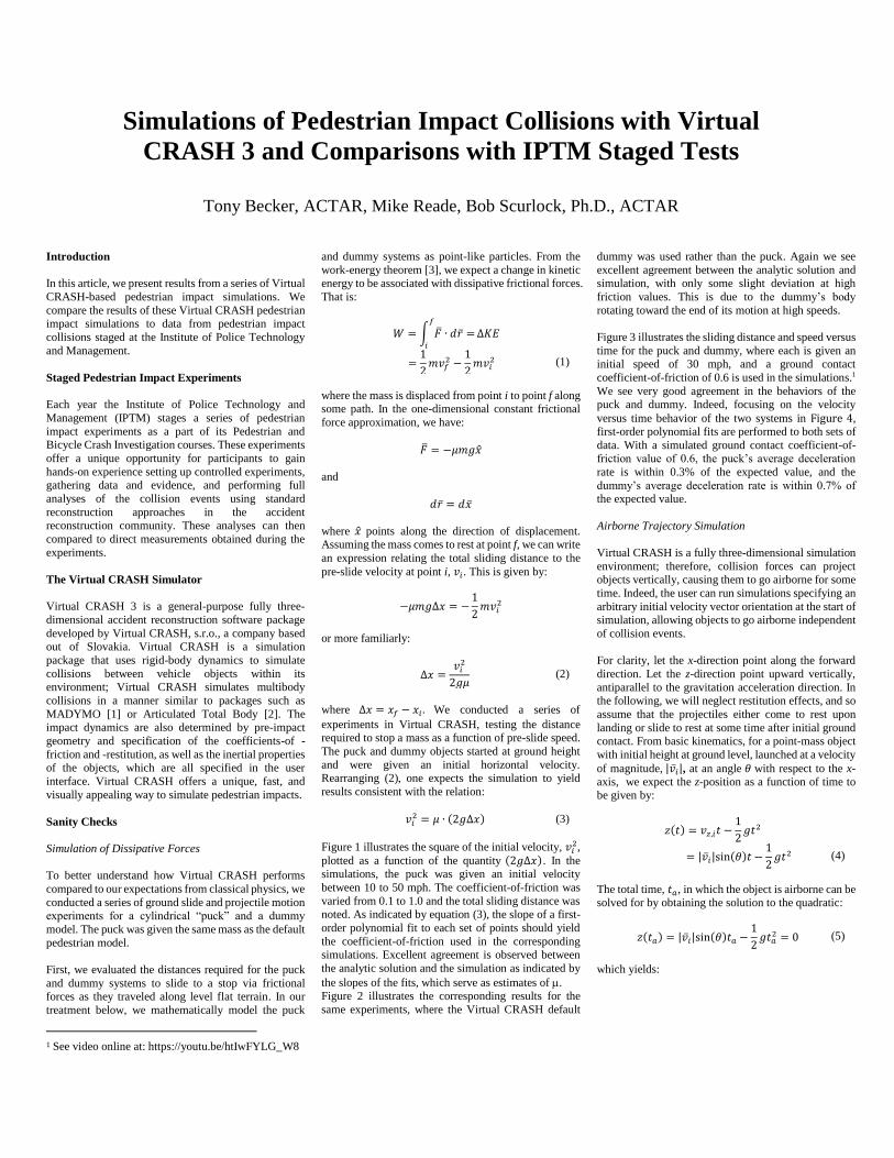
Figure 3 illustrates the sliding distance and speed versus

time for the puck and dummy, where each is given an initial speed of 30 mph, and a ground contact

coefficient-of-friction of 0.6 is used in the simulations.1

We see very good agreement in the behaviors of the puck and dummy. Indeed, focusing on the velocity

versus time behavior of the two systems in Figure 4, first-order polynomial fits are performed to both sets of

data. With a simulated ground contact coefficient-of-friction value of 0.6, the puck’s average deceleration

rate is within 0.3% of the expected value, and the

dummy’s average deceleration rate is within 0.7% of the expected value.

Airborne Trajectory Simulation

Virtual CRASH is a fully three-dimensional simulation

environment; therefore, collision forces can project objects vertically, causing them to go airborne for some

time. Indeed, the user can run simulations specifying an

arbitrary initial velocity vector orientation at the start of simulation, allowing objects to go airborne independent

of collision events.

For clarity, let the x-direction point along the forward

direction. Let the z-direction point upward vertically,

antiparallel to the gravitation acceleration direction. In the following, we will neglect restitution effects, and so

assume that the projectiles either come to rest upon

landing or slide to rest at some time after initial ground contact. From basic kinematics, for a point-mass object

with initial height at ground level, launched at a velocity

of magnitude, |�̅�𝑖|, at an angle 𝜃 with respect to the x-axis, we expect the z-position as a function of time to be given by:

𝑧(𝑡) = 𝑣𝑧,𝑖𝑡 −

1

2𝑔𝑡2

= |�̅�𝑖|sin(𝜃)𝑡 −1

2𝑔𝑡2 (4)

The total time, 𝑡𝑎, in which the object is airborne can be solved for by obtaining the solution to the quadratic:

𝑧(𝑡𝑎) = |�̅�𝑖|sin(𝜃)𝑡𝑎 −1

2𝑔𝑡𝑎

2 = 0 (5)

which yields:

𝑡𝑎 =2|�̅�𝑖|sin(𝜃)

𝑔 (6)

Figure 5 shows the total airborne time for simulated 30

mph launches of the puck and dummy systems as a

function of sin(𝜃).2 First-order polynomial fits to these data points yield slopes that estimate the quantity

2|�̅�𝑖|/g. Excellent agreement is observed between our analytic solution and simulation to the 1/100% level for

both systems.

Since the object undergoes uniform motion along the

horizontal direction (neglecting air resistance), we can

solve for the total horizontal airborne distance by:

𝐷𝑎 = 𝑣𝑥,𝑖𝑡𝑎 = |�̅�𝑖|cos(𝜃)𝑡𝑎

=2|�̅�𝑖|

2sin(𝜃) ∙ cos(𝜃)

𝑔 (7)

Equation (7), of course, is the famous range equation from classical physics.

Figure 6 illustrates the total airborne distance as a

function of the quantity (𝑠in(𝜃) ∙ cos(𝜃)) for 30 mph

launches of the puck and dummy systems. First-order polynomial fits to the data serve to estimate the quantity (2|�̅�𝑖|

2/𝑔) . Again, excellent agreement between the simulations and the analytic solution is observed to

better than a fraction of a percent.

Ground Contact

During the landing phase of projectile motion, the test

mass interacts with the ground such that a contact-force

is imparted to the mass, �̅�(𝑡), over a time ∆𝑡, which arrests the vertical motion of the mass and

simultaneously retards its horizontal velocity. The

impulse imparted to the test mass is given by [4]:

𝐽 ̅ = ∫ 𝑑𝑡 ∙ �̅�∆𝑡

0

= 𝑚∆�̅�

= ∫ 𝑑𝑡 ∙∆𝑡

0

𝐹𝑛�̂� + ∫ 𝑑𝑡 ∙∆𝑡

0

𝐹𝑡�̂� (8)

where �̂� is the unit vector pointing along the direction

normal to the surface of contact (ground), and �̂� points

in the direction orthogonal to �̂� . Along the normal-direction we have:

𝐽𝑛 = ∫ 𝑑𝑡 ∙∆𝑡

0

𝐹𝑛 = 𝑚∆𝑣𝑛 (9)

and along the tangent direction, we have:

𝐽𝑡 = ∫ 𝑑𝑡 ∙

∆𝑡

0

𝐹𝑡 = 𝑚∆𝑣𝑡

(10)

where ∆𝑣𝑛 and ∆𝑣𝑡 are the normal and tangent axis

projections of change-in-velocity vector ∆�̅� respectively. The “impulse ratio” is given by:

𝜇 =𝐽𝑡𝐽𝑛

(11)

2 A video of the 30 mph 40 degree launch is online at: https://youtu.be/3aSFtCC6y4c

Therefore, from (9), (10), and (11) we have:

∆𝑣𝑡 = 𝜇 · ∆𝑣𝑛 (12)

The sign of the impulse ratio is determined by the

relative velocity vector component tangent to the contact surface at the moment of contact. The impulse

ratio is typically associated with the inter-object surface

contact coefficient-of-friction, whose average behavior is often referred to as the drag factor. In this paper, we

use the terms interchangeably since we neglect any

time-dependent behavior of 𝜇.

The coefficient-of-restitution is given by the ratio of normal components of the final to initial relative

velocities at the point-of-contact.

𝜀 = −𝑣𝑅𝑒𝑙𝑛,𝑓

𝑣𝑅𝑒𝑙𝑛,𝑖 (13)

where the relative velocity is defined as the difference

between the velocity vectors of the two interacting objects at the point-of-contact:

�̅�𝑅𝑒𝑙 = �̅�1 − �̅�2 (14) The normal and tangent projections of this are given by:

𝑣𝑅𝑒𝑙𝑛 = �̅�𝑅𝑒𝑙 ∙ �̂� (15) and

𝑣𝑅𝑒𝑙𝑡 = �̅�𝑅𝑒𝑙 ∙ �̂� (16)

Finally, we can rewrite the normal change-in-velocity as:

Δ𝑣𝑅𝑒𝑙𝑛 = 𝑣𝑅𝑒𝑙𝑛,𝑓 − 𝑣𝑅𝑒𝑙𝑛,𝑖

= −𝜀 ∙ 𝑣𝑅𝑒𝑙𝑛,𝑖 − 𝑣𝑅𝑒𝑙𝑛,𝑖

or

𝛥𝑣𝑅𝑒𝑙𝑛 = −(1 + 𝜀) ∙ 𝑣𝑅𝑒𝑙𝑛,𝑖 (17)

and

𝛥𝑣𝑅𝑒𝑙𝑡 = −𝜇(1 + 𝜀) ∙ 𝑣𝑅𝑒𝑙𝑛,𝑖 (18)

Again, we treat the objects as point-like masses for our

simplified mathematical model. For two objects undergoing a collision, the change-in-relative-velocity

is related to the change-in-velocity at the center-of-

gravity of object 1 is given by the relation [4]:

∆�̅�1 = (�̅�

𝑚1

)∆�̅�𝑅𝑒𝑙 (19)

Here, the system’s reduced mass is given by:

�̅� =𝑚1 ∙ 𝑚2

𝑚1 +𝑚2

(20)

In the limit where the mass of object 2 becomes infinite (such in a ground impact), we have the following:

∆�̅�1 = ∆�̅�𝑅𝑒𝑙 (21)

𝛥𝑣𝑛 = −(1 + 𝜀) ∙ 𝑣𝑅𝑒𝑙𝑛,𝑖 (22)

𝛥𝑣𝑡 = −𝜇(1 + 𝜀) ∙ 𝑣𝑅𝑒𝑙𝑛,𝑖 (23)

Let us assume the ground is a flat level surface such �̂� =�̂� and �̂� = 𝑥 . Let object 1 be an object undergoing

projectile motion, and let object 2 be the infinitely

massive ground plane. In the no-restitution limit, we

have at time 𝑡𝑎 + ∆𝑡:

Δ𝑣𝑧 = |𝑣𝑧(𝑡𝑎)| (24)

and

Δ𝑣𝑥 = −𝜇 ∙ |𝑣𝑧(𝑡𝑎)| (25)

where the collision pulse width, ∆𝑡 , can be taken as

vanishingly small. Figure 7 illustrates the relation between the simulated horizontal changes-in-velocity

from and vertical changes-in-velocity for the puck and

dummy systems at the moment just after ground impact, after the downward vertical velocity has been arrested.

The plots in this figure were created using 30 mph

launch speeds at increasing launch angles between 5

degrees (lowest Δ𝑣𝑧) to 85 degrees (largest Δ𝑣𝑧) from horizontal. There are a few interesting features of note

in this figure. First, from equation (25), we expect a

first-order polynomial fit to yield a slope equal to the ground contact coefficient-of-friction used in the

simulations. This is indeed the case to within 0.4% for

the puck system and 6% for the dummy model. We also note in the dummy model simulations, when

Δ𝑣𝑧exceeds 15 mph (30 degrees), Δ𝑣𝑥 deviates from its

initial linear behavior. For Δ𝑣𝑧 > 25 mph we see a

dramatic drop in Δ𝑣𝑥 for the puck system.

For the dummy system, there are two effects that

explain the non-linear behavior. First, as the launch

angle increases, thereby increasing Δ𝑣𝑧 , the torque

imparted to the dummy’s body increases, causing an increase in rotational kinetic energy rather than a

decrease in linear kinetic energy. Therefore, we see a

slight reduction in the expected horizontal change-in-

velocity. In the second region, Δ𝑣𝑧 > 25 mph, we see the

same sharp reduction in Δ𝑣𝑥 as in the puck system. This

is related to the reduction in the maximum possible horizontal impulse that can be delivered to the objects,

which is naturally bounded such that the maximum

horizontal change-in-velocity cannot exceed the initial horizontal launch speed. This is further discussed below.

Post-Ground Contact

The vertical velocity component at first ground contact is given by:

𝑣𝑧,𝑓 = 𝑣𝑧,𝑖 − 𝑔𝑡𝑎

= |�̅�𝑖|sin(𝜃) − 𝑔 ∙2|�̅�𝑖|sin(𝜃)

𝑔 (26)

which simplifies to:

𝑣𝑧,𝑓 = −|�̅�𝑖|sin(𝜃) (27)

With this and equation (25), we can now solve for the

final ground speed after landing. This is given by:

𝑣𝑥,𝑓 = 𝑣𝑥,𝑖 + Δ𝑣𝑥

= |�̅�𝑖|cos(𝜃) − 𝜇|�̅�𝑖|sin(𝜃)

= |�̅�𝑖| ∙ (cos(𝜃) − 𝜇 ∙ sin(𝜃)) (28)

Assuming kinetic energy is dissipated through ground-

contact frictional forces, we can use equation (2) to solve for the total slide distance.

𝐷𝑆𝑙𝑖𝑑𝑒 =𝑣𝑥,𝑓2

2𝑔𝜇

=|�̅�𝑖|

2

2𝑔𝜇∙ (cos(𝜃) − 𝜇 ∙ sin(𝜃))

2 (29)

The total projectile travel distance is given by the sum of the sliding distance and the airborne travel distance;

that is:

𝐷𝑇𝑜𝑡𝑎𝑙 = 𝐷𝑎 +𝐷𝑆𝑙𝑖𝑑𝑒 (30)

or

𝐷𝑇𝑜𝑡𝑎𝑙 =2|�̅�𝑖|

2sin(𝜃) ∙ cos(𝜃)

𝑔

+|�̅�𝑖|

2 ∙ (cos(𝜃) − 𝜇 ∙ sin(𝜃))2

2𝑔𝜇

(31)

which simplifies to:

𝐷𝑇𝑜𝑡𝑎𝑙 =|�̅�𝑖|

2

2𝑔𝜇∙ (cos(𝜃) + 𝜇 ∙ sin(𝜃))

2 (32)

Figure 8 illustrates the total throw distance as a function

of the quantity (cos(𝜃) + 𝜇 ∙ sin(𝜃))2 for the puck and

dummy systems with 30 mph launch speeds and 𝜇 =0.6. The slope of a first-order polynomial fit yields estimates

of the quantity(|�̅�𝑖|2/2𝑔𝜇) . This estimate is within

0.05% of the expected value for the puck and within

0.6% for the dummy. Again, we see the deviation from the linear behavior for higher angles that is associated

with the expected reduction of horizontal impulse at

large launch angles. This is explored below.

Here we note that solving the above expression for |�̅�𝑖| yields the familiar Searle Equation:

|�̅�𝑖| =√2𝑔𝜇𝐷𝑇𝑜𝑡𝑎𝑙

cos(𝜃) + 𝜇 ∙ sin(𝜃) (33)

Returning to equation (32) above, taking the first

derivative gives:

𝜕𝐷𝑇𝑜𝑡𝑎𝑙𝜕𝜃

=|�̅�𝑖|

2

𝑔𝜇∙ (cos(𝜃) + 𝜇 ∙ sin(𝜃))

× (−sin(𝜃) + 𝜇 ∙ cos(𝜃))

(34)

Solving for the extremum values requires the following

relation to hold:

−sin(𝜃′) + 𝜇 ∙ cos(𝜃′) = 0 (35)

whose solution is given by:

tan(𝜃′) = 𝜇 (36)

To simplify the above expression, let:

cos(𝜃) =�̃�

√�̃�2 + �̃�2 (37)

and

sin(𝜃) =�̃�

√�̃�2 + �̃�2 (38)

Therefore, using (37) and (38), we have:

cos(𝜃) + 𝜇 ∙ sin(𝜃) =�̃� + 𝜇�̃�

√�̃�2 + �̃�2 (39)

The extremum condition above is now given by:

−�̃�′ + 𝜇 ∙ �̃�′ = 0 (40)

or,

cos(𝜃′) + 𝜇 ∙ sin(𝜃′) =

𝑥′̃ ∙ (1 + 𝜇2)

𝑥′̃√1 + 𝜇2= √1+ 𝜇2 (41)

Therefore, using (41), the total throw distance at angle

𝜃′, is given by:

𝐷𝑇𝑜𝑡𝑎𝑙(𝜃′) =|�̅�𝑖|

2

2𝑔𝜇∙ (√1 + 𝜇2)

2

=|�̅�𝑖|

2

2𝑔𝜇∙ (1 + 𝜇2) (42)

Checking the concavity at 𝜃′ , we apply the second derivative:

𝜕2𝐷𝑇𝑜𝑡𝑎𝑙𝜕2𝜃

=𝑣𝑖2

𝑔𝜇× {(−sin(𝜃′) + 𝜇 ∙ cos(𝜃′))

× (−sin(𝜃′) + 𝜇 ∙ cos(𝜃′))

+(cos(𝜃′) + 𝜇 ∙ sin(𝜃′))

+(cos(𝜃′) + 𝜇 ∙ sin(𝜃′))

× (−cos(𝜃′) − 𝜇 ∙ sin(𝜃′))} (43)

which simplifies to:

𝜕2𝐷𝑇𝑜𝑡𝑎𝑙𝜕2𝜃

(𝜃′) = −|�̅�𝑖|

2

𝑔𝜇√1 + 𝜇2< 0 (44)

Thus, the second derivative is negative definite,

implying that our function 𝐷𝑇𝑜𝑡𝑎𝑙(𝜃) at 𝜃′ is indeed a maximum value.

Limit on Horizontal Impulse

Let us now focus on the particular behavior of our test

mass just after ground impact. We know a retarding impulse is imparted to our mass upon ground impact;

this is given by equation (10). This tangent impulse will

only be applied so long as there is relative motion along the tangent axis direction between the interacting

objects at the point of contact. Once the relative motion

vanishes, this impulse component no longer acts on the mass. Therefore, the following relation must hold true

for our expression for 𝐷𝑇𝑜𝑡𝑎𝑙(𝜃) given by equation (32) to remain valid:

𝑣𝑥,𝑓 = |�̅�𝑖| ∙ (cos(𝜃) − 𝜇 ∙ sin(𝜃)) ≥ 0 (45)

This implies the condition:

cos(𝜃) − 𝜇 ∙ sin(𝜃) ≥ 0 (46)

There are two equivalent ways to interpret this

condition. First, we can solve for the angle, which gives

the solution to cos(𝜃) − 𝜇 ∙ sin(𝜃) = 0. This gives us a

boundary angle:

�̃� = tan−1 (1

𝜇) (47)

Therefore, when the launch angle satisfies the condition

𝜃 < �̃�, equation (32) holds. Otherwise, if the condition

is violated, the total distance is simply given by the range equation (7), where no sliding is expected. Thus,

we have:

𝐷𝑇𝑜𝑡𝑎𝑙 =

{

|�̅�𝑖|

2 ∙ (cos(𝜃) + 𝜇 ∙ sin(𝜃))2

2𝑔𝜇, 𝜃 < �̃�

2|�̅�𝑖|2sin(𝜃) ∙ cos(𝜃)

𝑔, 𝜃 ≥ �̃�

(48)

Figure 9 shows the total throw distance as function of

launch angle for 30 mph launches with 𝜇 =0.6 for both

puck and dummy systems. We see the simulated results track very closely to our analytic solutions. We also see

beyond the calculated boundary angle at 59 degrees, the

simulated behavior switches from following the Searle equation to the Range equation. Table 1 shows the

difference between the analytic solution and simulated

results. The simulated puck system shows better than 0.4% agreement and the dummy system shows better

than 4% agreement with the analytic solution given by

equation (48), each with much lower averages. This is

shown in Table 1.

We note here that the equation for �̃� has a dependence

on restitution that has been neglected in this treatment

and therefore will have different behavior when

generalized to account for this effect. This will be the

topic of a future article.

The second way to interpret equation (46), is as an upper

limit on the impulse ratio.

𝜇(𝜃) ≤ 1/tan(𝜃) (49)

That is, when using the Searle equation, one could use the following form for the coefficient-of-friction:

𝜇 = min(𝑓𝑑,1

tan(𝜃)) (50)

where 𝑓𝑑 is the measured or typical ground contact drag factor for the subject case. Let us suppose we know the

launch angle is sufficiently large such that we must use

𝜇(𝜃) = 1/tan(𝜃) (51)

Substituting (51) into equation (32) gives:

𝐷𝑇𝑜𝑡𝑎𝑙 = |�̅�𝑖|

2

2𝑔(1/tan(𝜃))

× (cos(𝜃) + (1/tan(𝜃)) ∙ sin(𝜃))2

=2|�̅�𝑖|

2sin(𝜃) ∙ cos(𝜃)

𝑔 (52)

which is simply equation (7), thereby indicating that

when the condition of no post-impact ground speed occurs, the total throw distance is simply given by the

classical range equation, as expected.

Figure 10 shows the launch speed as a function of total

throw distance for simulated launches between 10 and

50 mph, held at 20 degree launch angles. The coefficient-of-friction is set to 0.6. The corresponding

Searle curve from equation (33) is shown as well. The

Searle minimum and maximum curves are also drawn. Good agreement is evident between the Searle equation

and the simulated behavior as shown in Table 2. Note

there is no deviation from Searle behavior, as the 20 degree launch angle is well below the 59 degree

boundary angle given by equation (47).

Staged Collisions at IPTM

On August 12, 2015, a series of staged impacts were

conducted at the Institute of Police Technology and

Management at the University of North Florida. These

impacts were conducted as a part of the IPTM course on Pedestrian and Bicycle Crash Investigation. An aerial

view of the test site can be seen in Figure 11. During

these experiments, a plastic anthropomorphic dummy was impacted by a 2005 Ford Crown Victoria. The

dummy was 49 lbs in weight and measured 5.83 feet in height. Prior to impact, the dummy was suspended in an

upright position, using high-strength fishing line

attached to a boom (Figure 12). The boom was mounted to the rear of a truck offset from the collision path.

Upon impact, the fishing line broke free of the boom,

allowing the dummy to effectively interact with the vehicle structure, unimpeded. High-speed video footage

was captured of each collision event. Measurements of

the post-impact travel distance were recorded after each impact, as well as the average deceleration rate of the

2005 Ford Crown Victoria, which was made to hard

brake upon impact. The point of the dummy’s first ground contact was also carefully recorded (Figure 13).

The impact speed was also recorded for each test. A

summary of the test data is given in Table 3 and Figure 14. Participants of the 40 hour program conducted an

accident reconstruction analysis of each impact, based

on the total throw distance of the dummy. Reconstructed pre-impact vehicle speed estimates were

compared to known values recorded during each

collision.

Comparison of Staged Collision Data with Virtual

CRASH Dummy Behavior

A series of simulations were run in the Virtual CRASH

3 software environment. The simulated dummy’s height and weight were set to match that of the IPTM test

dummy described above. The simulated Crown Victoria

passenger vehicle weight was set equal to that of the IPTM test vehicle weight plus driver weight. The

simulated ground-contact coefficient-of-friction value

was set to the average measured at the scene (0.511), as was the vehicle-contact coefficient-of-friction (0.5). A

coefficient-of-restitution of 0 was used for both ground

and vehicle contact. Table 4 gives a summary of parameters used for the Virtual CRASH simulation runs.

3A video of this simulation and staged collision

footage can be seen online at: https://youtu.be/FM9W9SCteYc

The impact location along the Ford’s front bumper was

set to either 0.5 ft or 1.5 ft away from the center line, as this was not a well-controlled parameter during the

staged IPTM tests. The simulated dummy’s pre-impact

orientation was set to either 0 degrees (impact to rear of dummy) or 90 degrees (impact to left side of dummy).

Figure 15 depicts the moment-of-impact for two of the

simulated scenarios. It was found that there were no significant differences in the throw distances for

impacts to the simulated dummy’s left side compared to

right side.

From (48), we expect that the simulation should yield

the following relation:

|�̅�𝑖| ∝ √ 𝐷𝑇𝑜𝑡𝑎𝑙 (53)

Figure 16 illustrates the dependence of impact speed as

a function of √ 𝐷𝑇𝑜𝑡𝑎𝑙. First-order polynomial fits are

shown as well. Indeed, we see linear behavior over the

ensemble of the test runs for each given test scenario. Detailed summaries of the results are shown in Table 5

and Table 6. To quantify how well Virtual CRASH

simulates the dummy behavior observed in the IPTM staged tests, we calculate the differences (residuals)

between first-order polynomial fits to the Virtual

CRASH results and the test data. A plot of the residuals is shown in Figure 17. Here we see that the best match

to set of IPTM data is given by Scenario 3, where the

maximum deviation of the predicted impact speed based on total throw distance using Virtual CRASH

simulations is less than 3 mph when compared to the

IPTM dataset. Figure 18 depicts data from Scenarios 1 and 3, as well

as the Searle Minimum curve. The IPTM dataset is

shown. We also show the best fit to data for wrap trajectory impacts aggregated in the meta-analysis

presented by Happer et al., along with the

corresponding 85% prediction interval [5]. Here we see excellent agreement between Virtual CRASH simulated

impacts, IPTM data, and expectations from prior studies.

Simulating Gross Behavior of Test Dummy

In addition to simulating the total throw versus impact speed behavior of the test data, we wanted to see if we

could simulate the overall behavior of the test dummy’s

motion using Virtual CRASH. The height and weight of the crash test dummy were both input into Virtual

CRASH. The joint stiffness properties of the Virtual

CRASH simulated dummy can be adjusted such that the user can tune the dummy’s overall rigidity. This can be

done separately for each joint if needed. We chose to

focus on adjusting three of the dummy parameters to get reasonable agreement between behavior observed in the

staged collision 4 video and the Virtual CRASH output:

these parameters were the overall coefficient-of-restitution, coefficient-of-friction, and joint stiffness.

These values were tuned until overall gross behavior

was observed to match that of the staged experimental dummy. The sequence can be seen in Figure 19 for

IPTM crash test 4.3 As expected, we found that one can

optimize the Virtual CRASH settings until the overall

simulated behavior is in good agreement with the

observed behavior during staged tests.

Conclusions

We have tested Virtual CRASH for use in modeling

pedestrian impacts. The simulator faithfully reproduces

the expected behavior of projectiles during both the airborne and ground sliding phases of their trajectories.

The throw distances as a function of impact speed

behavior of the simulated dummy model does a good job reproducing the behavior observed during staged

impact experiments as well as that which was observed

in prior experiments.

About the Authors

Tony Becker has conducted extensive research in

pedestrian and cyclist traffic crash investigation and

published several articles and books that are widely

used in the field. He is an ACTAR certified accident

reconstructionist and trainer in Florida. He can be

contacted at beckercrash@gmail.com.

Mike Reade, CD is the owner of Forensic

Reconstruction Specialists Inc., a collision reconstruction consulting firm located in Moncton, New

Brunswick Canada. He is also an Adjunct Instructor with the Institute of Police Technology and

Management – University of North Florida (IPTM-

UNF) based out of Jacksonville, Florida. He can be reached at reademw@gmail.com.

Bob Scurlock, Ph.D., ACTAR, is the owner Scurlock Scientific Services, LLC, an accident reconstruction

consulting firm based out of Gainesville, Florida, USA.

He is also a Research Associate at the University of Florida, Department of Physics. His website can be

found at www.ScurlockPhD.com. He can be reached at

BobScurlockPhD@gmail.com.

References

[1] “The Pedestrian Model in PC-Crash – The

Introduction of a Multi-Body System and its

Validation”, A. Moser, H. Steffan, and G. Kasanicky. SAE 1999-01-0445.

[2] “Articulated Total Body Model Enhancements,

Volume 2: User’s Guide”, L. Obergelfell et al. Report

No. AAMRL-TR-88-043 (NTIS No. A203-566).

[3] “Classical Dynamics of Particles and Systems”, J. Marion and S. Thornton, Harcourt College Publishers,

New York, New York, 1995.

[4] “Rigorous Derivations of the Planar Impact

Dynamics Equations in the Center-of-Mass Frame”, B. Scurlock and J. Ipser, Cornell University Library

arXiv:1404.0250.

[5] “Comprehensive Analysis Method for

Vehicle/Pedestrian Collisions”, A. Happer et al. SAE 2000-01-0846.

Figure 2: Results from dummy slide-to-stop experiments in Virtual CRASH.

Figure 1: Results from puck slide-to-stop experiments in Virtual CRASH.

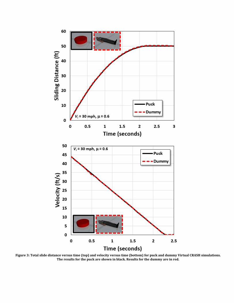
Figure 3: Total slide distance versus time (top) and velocity versus time (bottom) for puck and dummy Virtual CRASH simulations.

The results for the puck are shown in black. Results for the dummy are in red.

Figure 4: Velocity versus time for Puck (top) and Dummy (bottom) versus time. First-order polynomial fits yield the decelerations

rates for the simulation.

Figure 5: Total airborne time for puck (top) and dummy (bottom). First-order polynomial fits are shown.

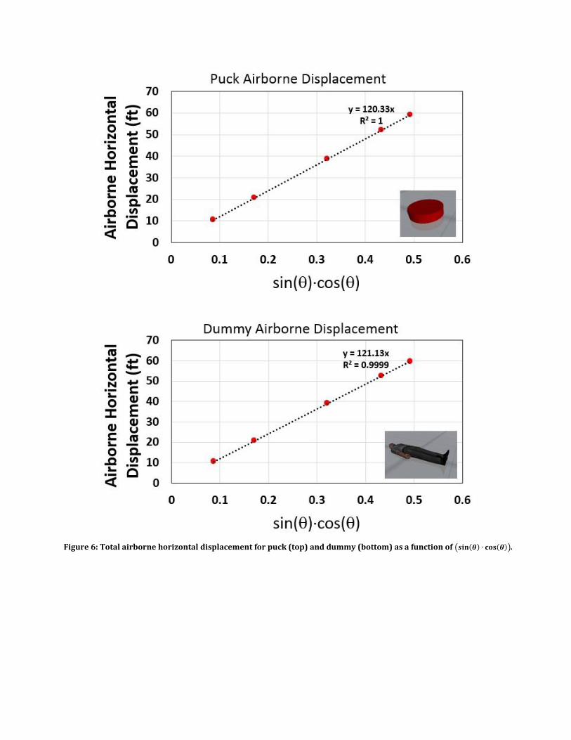
Figure 6: Total airborne horizontal displacement for puck (top) and dummy (bottom) as a function of (𝒔𝐢𝐧(𝜽) ∙ 𝐜𝐨𝐬(𝜽)).

Figure 7: 𝚫𝒗𝒙versus 𝚫𝒗𝒛 for the puck (top) and dummy (bottom) systems. First-order polynomial fits are performed to the linear

region (open circles).

Figure 8: Total throw distance for puck (top) and dummy (bottom). First-order polynomial fits are performed to the linear region

(open circles).

Figure 9: Total throw distance as a function of launch angle for puck and dummy systems.

Table 1: Difference between analytic solution and simulation for the puck (top) and dummy (bottom) systems.

Figure 10: Launch speed estimates as a function total throw distance. Results from puck and dummy simulations are shown for a 20

degree launch.

Table 2: Differences between analytic solution of estimated launch speed and simulations of puck and dummy systems for a 20 degree launch.

Figure 11: Aerial view of test site at IPTM.

Figure 12: Anthrophonic test dummy pre-impact configuration.

Figure 13: Dummy post-impact position.

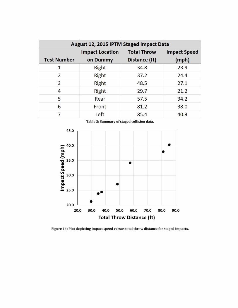
Table 3: Summary of staged collision data.

Figure 14: Plot depicting impact speed versus total throw distance for staged impacts.

Table 4: Summary of simulation input parameter settings used in Virtual CRASH 3.0.

Figure 15: Moment-of-impact depicted for Scenario 1 (left) and Scenario 4 (right).

Figure 16: Plots depicting relationship between Impact Speed and the square root of the total throw distance. Plots are shown for the

four simulated scenarios. The IPTM test data is plotted as well.

Table 5: Summary of results for simulation Scenarios 1 (top) and 2 (bottom).

Table 6: Summary of results for simulation Scenarios 3 (top) and 4 (bottom).

Figure 17: Plot of residuals as a function of simulation fit values for all four Scenarios.

Figure 18: Plot depicting impact speed versus square root of total throw distance for Scenarios 1 and 3.

Figure 19: Comparing simulation of Test #4 of IPTM staged impact.