simulations of water-air flows with low and high … of water-air flows with low and high pressure...

University Bulletin – ISSUE No.19- Vol. (3) – July - 2017. 87

Simulations of Water-Air Flows with Low and High

Pressure Ratios

Dr. Shaban Jolgam 1

, Dr. Ahmed Ballil2, and Dr Andrew Nowakowski

3

1Dept. of Mechanical engineering, Zawia University

2Dept. of Mechanical engineering, Benghazi University,

3Dept. of Mechanical engineering, Sheffield University, Sheffield, UK

Abstract:

Numerical simulation of two phase flows, which includes interface

creation and evolution, is a challenging task due to its complexity. In this

contribution, simulations of water-air flows characterised by high and low

pressure jumps across the interface are presented. A computer program

using "C" language is developed to compute a fully non-equilibrium two-

phase flow model. The model consists of seven partial differential

equations in one dimensional flow as follows: mass, momentum and energy

equations for each constituent augmented by a volume fraction evolution

Simulations of Water-Air Flows with Low and High Pressure Ratios ــــــــــــــــــــــــــــــــــ


equation for one of the constituents. A diffuse interface numerical method

is employed to capture the interface evolution in different water-air flow

regimes. This method is based on an extended second order finite volume

Godunov-type approach. A fixed Eulerian mesh is built and fluxes at each

cell boundaries are computed using an efficient HLL approximate Riemann

solver. Velocity and pressure relaxation procedures are applied to fulfill

the interface conditions. Two case studies are considered to verify the

developed code. The first case considers the water-air shock tube problem,

which provides a high pressure ratio of (104) and the second test considers

the water-faucet flow, which provides a low pressure ratio of (1). The

obtained results show very good agreement with both the exact solutions

and other published results.

Keywords: compressible multiphase flow, hyperbolic PDEs,

Riemann problem, Godunov methods, shock waves, HLL Riemann solver.

1. Introduction:

Numerical modeling of multiphase flows has been developed

enormously in recent years. In this context, many mathematical models

have been derived and many numerical approaches have been developed

and applied to represent the complex physics of multiphase flows. This

paper is concerned with the numerical simulation of multiphase flows, in

particular water-air flows. These flows are common in many natural

phenomena, hydraulic engineering and industrial applications. For

example, rain, bubbly flows, cavitations' phenomenon, water jet flows,

thermal and chemical plants.

Many investigations were conducted to study the physical behavior

of different air-water flow regimes. For instance, the air-water flow field

ـــــــــــــــــــــــــــــــــــــــــــــــــــــــــــــــــــــــــــــــــــــــــــــــــــــــــــــــــ Dr. Shaban Jolgam & et.al.,


which includes air bubble sizes, air bubble distributions, air-water velocity

profiles and bubble-turbulence interactions was studied and analyzed in the

theme of air entrainment processes in free-surface turbulent flows in [1].

The two phase air-water flows in vertical capillary tubes were studied and

some flow characteristics such as void fraction, frictional pressure loss and

rise velocity of slug bubbles were measured in [2]. Numerical simulations

of multiphase air-water flows through high pressure nozzles were presented

in [3]. Recently, Air-water interactions in hydraulic jump were simulated

using a mesh-free particle (Lagrangian) method in [4].

Numerically, there are two main approaches that are widely used to

simulate multiphase flows including air-water flows. These are: Sharp

Interface Methods (SIM) and Diffuse Interface Methods (DIM). The SIM

methods consider interfaces between flow constituents as sharp non-

smeared discontinuities. consequently, the approaches under this category

eliminating numerical diffusion at the interfaces completely, which means

the artificial mixing problem is eliminated as well. This is the main

advantage of the SIM over the DIM, however, other numerical and

practical difficulties may possibly occur. Some well-known examples of

these methods are the interface tracking methods [5], arbitrary Lagrangian-

Eulerian methods [6], volume of fluid methods [7,8] and level set

methods[9].

On the other hand, the DIM methods allow numerical diffusion at the

interface. Although numerical diffusion is considered as a weakness for

numerical methods, it is an essential feature for capturing any flow

discontinuities. There are a number of ways to reduce the effect of

numerical diffusion at the interface. For example, mesh refinement and

using high order numerical schemes. Nevertheless, these methods are



relatively easier and more flexible in coding and implementation than SIM.

The DIM mainly divided into two groups of methods: the first group is

based on Euler equations as presented for example in [10,11]. These

methods are easy to implement and very efficient for simulating flows with

relatively simple physical problems. However, they suffer the lake of

accuracy in computing internal energies and temperatures at interfaces. The

second group is based on multiphase flow equations. These models are

more suitable for solving multiphase flow problems than the Euler

equations. They are able to deal with general equations of state,

conservative for mixtures and provide precise internal energies and

temperatures at interfaces. Good examples of these models are the parent

model developed in [12], the transport multiphase model proposed in [13],

the reduced multiphase model derived in [14] and the six equation model

developed in [15,16].

In this work the hyperbolic, non-equilibrium, multiphase flow model

that presented in [17] is adopted to simulate different air-water flow

regimes. A numerical framework based on Godunov type approach is

implemented within a newly developed "C" language code. Both velocity

and pressure relaxation terms are taken into account during the

computations. The main challenge is to simulate the water-air flows with

low and high pressure jumps across the interface.

This paper is organized as follows: The mathematical formulation of

the governing equations of the two-phase flow models are reviewed in the

next section. Then the numerical method is described with the HLL

Riemann solver. After that, the case studies and obtained results are

presented. Finally, the conclusions are derived.



2. Mathematical formulation:

For most two-phase flow problems with interfaces that move and

deform, the local instant formulation based on the single-phase equations

encounters mathematical and numerical difficulties. Hence, a suitable

averaging method has become essential to continuously eliminate

interfacial discontinuities and make a two-phase flow as a continuum

formulation [18].

A compressible two-phase flow model can be obtained by applying

the averaging method of Drew presented in [19] to the Navier-Stokes

equations for single-phase flow. Saurel and Abgrall in [12] have developed

a multiphase flow model by applying this method and considering all

dissipative terms at the interfaces and neglecting them everywhere else.

Their model, which is known later as the parent model, was inspired by the

work of Baer and Nunziato which was presented in [20]. The model of

Baer and Nunziato was proposed to study the deflagration-to-detonation

transition in solid energetic materials. The model of [12] is similar to that

of [20] but they have introduced different treatments of the interfacial

variables and relaxation parameters. These treatments have extended the

range of applications of the parent model which can be written in one

dimension without heat and mass transfer terms in the following form:

211

int1 pp

xu

t

(1a)

011111

x

u

t

(1b)

guu

xp

x

pu

t

u1112

1int

11

2

111111

(1c)



12int

1intint

111111111 uuux

upx

pEu

t

E

guppp 11121int (1d)

022222

x

u

t

(1e)

guu

xp

x

pu

t

u2212

1int

22

2

222222 -

(1f)

12int

1intint

222222222 uuux

upx

pEu

t

E

guppp 22221int (1g)

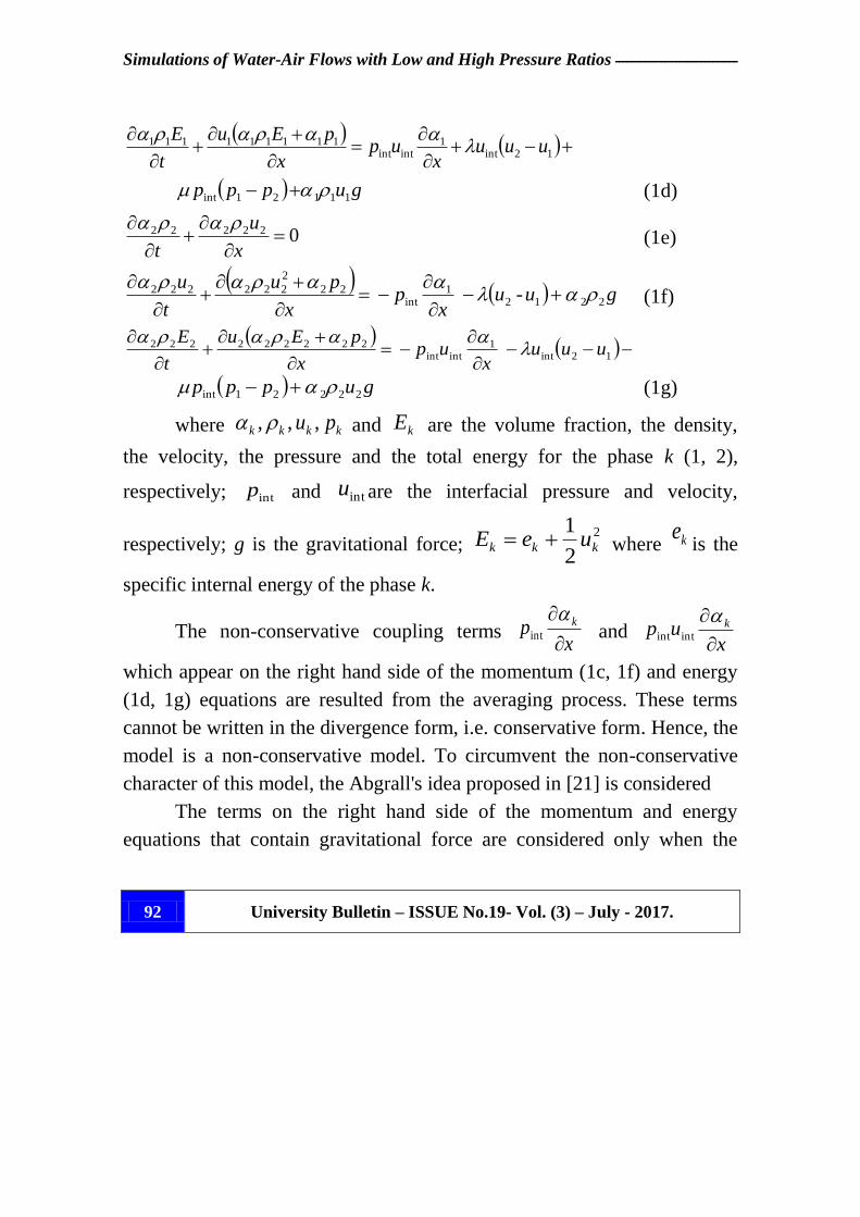
where , , , kkkk pu and kE are the volume fraction, the density,

the velocity, the pressure and the total energy for the phase k (1, 2),

respectively; intp and intu are the interfacial pressure and velocity,

respectively; g is the gravitational force; 2

2

1kkk ueE where ke

is the

specific internal energy of the phase k.

The non-conservative coupling terms x

p k

int and

xup k

intint

which appear on the right hand side of the momentum (1c, 1f) and energy

(1d, 1g) equations are resulted from the averaging process. These terms

cannot be written in the divergence form, i.e. conservative form. Hence, the

model is a non-conservative model. To circumvent the non-conservative

character of this model, the Abgrall's idea proposed in [21] is considered

The terms on the right hand side of the momentum and energy

equations that contain gravitational force are considered only when the



gravity has a significant effect such as in the water- faucet test, which is

conducted in this work.

2.1 Closure relations:

Extra terms, which represent the transfer processes that may take

place at the interface, appear in the model result from the averaging process

used to derive the model (1). These terms are unknown. Volume fractions,

which are known and indicate the presence of each phase within the

computational cell, for each phase also appear on the right hand side of the

model (1). Originally the multiphase flow model (1) consists of two mass

equations (1b, 1e), two momentum equations (1c, 1f) and two energy

equations (1d, 1g). The number of these equations is six which is less than

the number of the unknown variables which are twelve. Therefore, the

following relations are considered to close the model (1):

Evolution equation for volume fraction (1a) is added to the model (1)

as proposed by [22].

Volume fraction constraint which may be written as follows:

1 21 (2)

Equations of state are used to link the thermodynamic variables

within each phase. In this work stiffened equation of state is considered to

govern the working fluids. The stiffened equation of state may be written in

the following form:

ep 1 (3)

where

is the adiabatic specific heat ratio and is the pressure

constant they depend on the material under consideration.

The interfacial pressure is assumed to be equal to the mixture

pressure [12]:



k kkpp int (4)

The interfacial velocity is assumed to be equal to the mixture

velocity [12]:

k kk

k kkk uu

int (5)

2.2 Pressure relaxation terms:

The pressure relaxation term 21 pp which appears on the right

hand side of the volume fraction evolution equation (1a) expresses the

expansion rate of the volume fraction. The expansion rate drives the

pressure to equilibrium. The other pressure relaxation term 21int ppp

which appears on the right hand side of the energy equations (1d, 1g)

expresses the pressure work done by the phases to achieve the pressure

equilibrium. The variable controls the rate at which the pressure

relaxation process takes place; its value grows to be infinite at the interface

in order the process takes place in a short time [17].

2.3 Velocity relaxation terms:

The velocity relaxation terms 12 uu and 12int uuu which

appear on the right hand side of the momentum equations (1c, 1f) and

energy equations (1d, 1g), respectively, are responsible for driving both

phases to relax to a common velocity at the interface. The value of the

variable has to be infinite increase the rate at which the velocity

relaxation process takes place rapidly [17].



3. Numerical method:

The exact analytical solution of the multiphase flow model (1) is

unknown [23]. Therefore, the only choice is to solve it numerically.

However, the numerical solution of this model is not easy due to the

presence of the non-conservative equation of the evolution of volume

fraction (1a), the non-conservative terms existing on the right hand side of

the momentum equations (1c, 1f) and energy equations (1d, 1g) and the

relaxation term that appear on the right hand side of the model as

mentioned earlier. Therefore, numerical solution can be attained by

splitting the model into hyperbolic part operator t

hL and source and

relaxation part operator t

sL and solving them using the Strang splitting

technique which may be written in second order as follows:

n

i

t

s

t

h

t

s

n

i ULLLU 221 (6)

where 1n

iU and n

iU are the vectors of conservative variables at

times 1n and n , respectively. The hyperbolic part and source and

relaxation part operators have to be solved in succession as given in [17].

3.1 The hyperbolic operator:

The hyperbolic part of the two-phase flow model (1) can be written

as follows:

0 1int

1

xu

t

(7a)

xUH

x

UF

t

U

1 )( )(

(7b)



where U , UF and UH are the vectors of conserved variables,

fluxes and non-conservative, they are given respectively as follows:

.

0

0

and ,

int

int

intint

222222

22

2

222

222

111111

11

2

111

111

222

222

22

111

111

11

i

i

up

p

up

p

UH

pEu

pu

u

pEu

pu

u

UF

E

u

E

u

U

The solution of the hyperbolic system (7) is not direct as for the

Euler equations due to the existence of the non-conservative equation (7a)

of the volume fraction. The solution can be attained by applying the

Godunov-type scheme which is used to discretise the non-conservative

system (7). To obtain a second order accuracy in time and space the

MUSCL scheme is applied [24]. The discretisation of the system (7) can be

written as follows:

),(),( 2121

*

2121

*1

iiiii

n

i

n

i ux

t (8a)

)),(( 2121

*1

ii

n

i

n

i UUUFx

tUU

i

n

iii UHtUUUF

)()),(( 21

2121

* (8b)

where F is the numerical flux vector calculated at the intercell

boundaries 21ix between

21iU and

21iU , i is the discretization of the

volume fraction x

1 in space which depends on the approximate Riemann



solver [17] and )( 21n

iUH is the vector of non-conservative terms. The time

step is computed using the following expression:

Max

CFL

S

xt

(9)

where CFL is the Courant number; for stability it has to be less than

one, x is the cell size and SMax is the maximum wave speed. The left and

right wave speeds at the boundaries

21iS and

21iS can be computed for

the two phases respectively by:

),,(min 21,21,21,21,21

ikikikiki cucuS (10a)

),,(max 21,21,21,21,21

ikikikiki ucucS (10b)

where k represents the phases 1 and 2.

3.2 The HLL approximate Riemann solver:

This approximate Riemann solver which is presented in [25] is based

on a minimum S and maximum

S wave speeds arising in the Riemann

solution. The solver uses a single intermediate state (*) enclosed between

these two waves. According to this solver the fluxes may be computed

using the following expression:

.0 if

,0 if

,0 if

21

2121

21

2

11

iR

ii

hll

iL

hll

SF

SSF

SF

F (11a)

2121

21212121

21

ii

LRiiRiLihll

iSS

UUSSFSFSF . (11b)



According to the HLL solver the discretization of the volume

fraction equation (8a) in space and time may be rewritten as follows:

2121

21

,21

21

,212121

2121

21

,2121

21

,2121

21

1)()(

ii

n

i

n

iii

ii

n

ii

n

ii

n

in

i

n

iSS

SS

SS

SSu

x

t

2121

21

,21

21

,212121

2121

21

,2121

21

,2121

21 )()(

ii

n

i

n

iii

ii

n

ii

n

ii

n

i

SS

SS

SS

SSu (12)

and the discretization of the volume fraction in space i in the

equation (8b) according to the HLL solver may be written as follows:

2/112/11

2/1

,2/12/11

2/1

,2/12/11

2/112/11

2/1

,2/12/11

2/1

,2/12/111

SS

SS

SS

SS

x

n

i

n

i

n

i

n

i

i

(13)

3.3 The relaxation and source terms operator :

The relaxation and source terms operator part of the two-phase flow

model (1) is an ordinary differential equations ODE which can be written

as follows:

SPV DDDdt

dQ , (14)

where Q, DV, DP, DS represent the volume fraction and the conserved

variables, the velocity relaxation parameters, the pressure relaxation

parameters and the source terms, respectively, They are defined as follows:

(15) .

0

0

0

and

)(

0

0

)(

0

0

)(

,

)(

)(

0

)(

)(

0

0

,

222

22

111

11

21int

21int

21

12int

12

12int

12

222

222

22

111

111

11

1

gu

g

gu

g

D

ppp

ppp

pp

D

uuu

uu

uuu

uu

D

E

u

E

u

Q SPV



The solution of the ODE (14) is obtained by solving the integration

operators using the Strang method:

n

i

t

s

t

P

t

V

n

i QLLLQ 1 (16)

where the operators LV, LP, LS are defined by the vectors DV, DP, DS,

respectively, given by (15). Internal energy for both phases must be

updated after velocity relaxation process. Velocity and pressure relaxation

processes have to be done every time step. The effect of gravity is

considered by solving the source term operator when it has a significant

effect.

4. Test problems and results:

The assessment of the performance of the developed algorithm was

carried out using carefully chosen test problems. These test problems

represent two different test cases where the pressure ratio between the two

flow constituents varies from a very high pressure ratio of (104) to a very

low pressure ratio of (1). A necessary assumption is usually made for

numerical simulations of two-phase flows using diffuse interface methods.

The assumption is that a presence of a negligible volume fraction ɛ = 10-8

of the second phase in the first phase which is considered as a pure phase.

4.1 Water-air shock tube:

This is a standard water-air shock tube test problem used to assess

the ability of the developed code to simulate problems with flow

constituents that have very high pressure ratios. The tube is 1 m long and

divided to two chambers. The left hand chamber is filled with water at a

higher pressure and the right hand chamber is filled with air at atmospheric

pressure. The interface which separates the two fluids is located at x = 0.7



m. Both fluids are governed by the stiffened gas equation of state. The

stiffened gas equation of state parameters for air are 4.1 , Pa 0 and

for water are 4.4 , Pa 106 8 . The initial conditions for both

components are:

.7.0 if 10,0,50

,7.0 if 10,0,1000,,

5

9

x

xpu (17)



Figure 1. Water-air test: Surface plot for time evolution for: (a) pressure, (b)

velocity, (c) mixture density and (d) volume fraction.

Initially both constituents are at rest, as soon as the membrane

separating the two components is removed, the water which has the higher

pressure and density starts to move to the right. Therefore, strong shock

and contact discontinuity waves are generated which move to the right and

a rarefaction wave is generated which moves to the left. The numerical



results are obtained from the HLL approximate Riemann solver using 200

cells with the CFL = 0.9. The surface and contour plots for the results of

time evolution for pressure (a), velocity (b), mixture density (c) and volume

fraction (d) are show in Figure 1 and Figure 2, respectively. One can notice

clearly the shock and rarefaction waves from the velocity contour plot (b)

in Figure 2.



Figure 2. Water-air test: Contour plot for time evolution for: (a) pressure, (b)

velocity, (c) mixture density and (d) volume fraction.



Figure 3. Water-air test: results of (a) pressure, (b) velocity, (c) mixture density

and (d) volume fraction at t = 229 µs.

The results of pressure (a), velocity (b), mixture density (c) and

volume fraction (d) for this test are obtained using 1000 cells and compared

to the exact solution at t = 229 µs as shown in Figure 3. It can be observed

that the results are in a good agreement with the exact solution.

4.2 Water-faucet test:

This test was proposed by Ransom in [26] to study behavior of

incompressible two-phase flows. The test is chosen to be simulated using

the model (1) which was basically proposed for compressible two-phase



flows. The test consists of a vertical tube with open ends. The tube depth is

12 m and contains of a water column which is surrounded by air. The water

leaves the faucet and enters the tube at atmospheric pressure with velocity

of m/s 10 and volume fraction of 0.8. Several stages are presented in Figure

4. Under the effect of gravity, the water accelerates and narrows as it passes

through the tube to maintain mass conservation. Therefore, the

gravitational effect is considered in the calculations for this test. At the

interface, which separates the flow components, each component has

different direction and hence the velocity relaxation is not performed in the

numerical solution of this test.

Figure 4. Water-faucet test.

The initial conditions are as follows:

.Air 0.2 ,10,0,1

,Water 0.8 ,10,10,1000,,,

5

5

pu (18)

The stiffened gas equation of state parameters are 4.1 , Pa 0

for air and 4.4 , Pa 106 6 for water.

The water-faucet test is used to assess developed numerical

algorithms as it has an analytical solution. The analytical solution could be



derived by neglecting the pressure variation in liquid and interfacial drag

between phases and assuming that the two components are incompressible.

The analytical solutions for the water velocity and the evolution of the air

volume fraction can be written as follows:

otherwise, g

,g2

1 if 2g)(

),(0

2

20

2

20

2

2

tu

ttuxxutxu (19)

otherwise.

,g2

1 if

2g)(1

),(

0

1

20

220

2

0

2

0

2

1

ttux

xu

u

tx (20)

Simulations of this test are conducted using the CFL = 0.6 and the

results are obtained at t = 0.4 s. Various mesh resolutions have been used to

show the convergence of the numerical solution. The results of the air

volume fraction and water velocity are shown in Figure 5. One can observe

that increasing the resolution more than 1500 cells would not improve

much the results as an overshot starts to grow as shown in Figure 5 (a). The

same observation can be seen in the results of Saurel and Abgrall 1999a.

Figure 5. Water-faucet test: results using different mesh resolutions at t = 0.4 s for

(a) air volume fraction and (b) water velocity.



5. Conclusions:

In this paper, the implementation of the DIM for two-phase flow

based on an extended second order finite volume Godunov-type approach

is done successfully. The assessment of the performance of the developed

algorithm has been verified for high and low pressure regimes using

benchmark test problems. Obtained results are in good agreement with the

exact solution for water-air test and water-faucet test. However, overshot

appears in the results of water-faucet test when very high number of cells is

used.

6. References:

[1] Chanson, H. (1997). Air Bubble Entrainment in Free-Surface

Turbulent Shear Flows. Academic Press, London, UK, (ISBN 0-12-

168110-6).

[2] Mishima, K. and Hibiki, T. (1996) Some Characteristics of Air-water

Two-phase Flow in Small Diameter Vertical Tubes. International

Journal of Multiphase Flow, Volume 22, Issue 4, 703-712.

[3] Jolgam, S. A., Ballil, A. R., Nowakowski, A. F. and Nicolleau, F. C. G.

A. (2012). Simulations of Compressible Multiphase Flows Through a

Tube of Varying Cross-section. Proc. The ASME 2012 11th Biennial

Conference on Engineering Systems Design and Analysis, Nantes,

France.

[4] Shakibaeinia, A. (2015). Mesh-free Particle Modelling of Air-water

Interaction. Proc. The 36th IAHR World Congress, Hague,

Netherlands.



[5] Cocchi, J. P. and Saurel, R. (1997). A Riemann Problem Based

Method for Compressible Multifluid Flows. Journal of Computational

Physics. Volume 137, 265-298.

[6] Farhat, C. and Roux, F. X. (1991). A Method for Finite element

Tearing and Interconnecting and its Parallel Solution Algorithm.

International Journal of Numerical Methods in Engineering. Volume

32, Issue 6, 1205-1227.

[7] Hirt, C. W. and Nichols, B. D. (1981). Volume Of Fluid (VOF) method

for the dynamics of free boundaries. Journal of Computational


[8] Youngs, D. L. (1982). Time Dependent Multi-material Flow with Large

Fluid Distortion (ed. K. W. Morton and M. J. Baines).Academic.

[9] Fedkiw, R. P., Aslam, T., Merriman, B. and Osher, S. (1999). A non

Oscillatory Eulerian Approach to Interfaces in Multimaterial Flows

(The Ghost Fluid Method). Journal of Computational Physics. Volume

152, 457-492.

[10] Karni, S. (1996) Hybrid Multifluid Algorithms. SIAM Journal of

Scientific Computing. Volume 17, Issue 5, 1019-1039.

[11] Shyue, K. M. (1998). An Efficient Shock-capturing Algorithm for

Compressible Multicomponent Problems, Journal of Computational


[12] Saurel, R. and Abgrall, R. (1999). A Multiphase Godunov Method for

Compressible Multifluid and Multiphase Flows. Journal of

Computational Physics. Volume 150, 425-467.

simulations of water-air flows with low and high … of water-air flows with low and high pressure...

Documents