simultaneous coupling of fluids and deformable bodies

Eurographics/ ACM SIGGRAPH Symposium on Computer Animation (2006)M.-P. Cani, J. O’Brien (Editors)

Simultaneous Coupling of Fluids and Deformable Bodies

Nuttapong Chentanez Tolga G. Goktekin Bryan E. Feldman James F. O’Brien

University of California, Berkeley

AbstractThis paper presents a method for simulating the two-way interaction between fluids and deformable solids. Thefluids are simulated using an incompressible Eulerian formulation where a linear pressure projection on the fluidvelocities enforces mass conservation. Similarly, elastic solids are simulated using a semi-implicit integratorimplemented as a linear operator applied to the forces acting on the nodes in Lagrangian formulation. Theproposed method enforces coupling constraints between the fluid and the elastic systems by combining both thepressure projection and implicit integration steps into one set of simultaneous equations. Because these equationsare solved simultaneously the resulting combined system treats closed regions in a physically correct fashion, andhas good stability characteristics allowing for relatively large time steps. This general approach is not tied to anyparticular volume discretization of fluid or solid, and we present results implemented using both regular-grid andtetrahedral simulations.

Categories and Subject Descriptors (according to ACM CCS): I.3.5 [Computer Graphics]: Computational Geometryand Object Modeling, Physically Based Modeling; I.3.7 [Computer Graphics]: Three-Dimensional Graphics andRealism, Animation; I.6.8 [Simulation and Modeling]: Types of Simulation, Animation

Keywords: Natural phenomena, physically based animation, computational fluid dynamics, two-way coupling,deformable bodies.

1. Introduction

The interaction between a fluid and deformable body cancreate complex and interesting motion that would be difficultto convincingly animate by hand. In this work we present amethod to solve for the interaction by simultaneously con-serving the momentum of the fluid and deformable bodywhile enforcing the conservation of fluid mass.

Previous approaches for coupling fluid and deformablebodies use a time splitting procedure. They alternately fixthe fluid pressure when simulating the solid, then fix thesolid’s velocity when simulating the fluid. While this ap-proach works reasonably well for physical systems withnon-stiff coupling, it can lead to instability and visual arti-facts for other systems. These problems occur because whilesolid velocities are fixed they will ignore arbitrarily largefluid pressures, and the converse when the fluid velocitiesare fixed. For a tightly coupled system like a water balloonwhere small changes in the state of the solid cause nearlyinstantaneous changes in the fluid and vice versa, time split-ting becomes untenable and difficulties can still arise evenfor less tightly coupled systems. Time splitting also createsproblems for systems that include fluid regions completely

Figure 1: A sequence of images showing a jet of smokeinteracting with multiple thin rubber sheets

surrounded by a deformable body. The volume of these re-gions can change during the solid simulation. In this case ap-plying Neumann boundary conditions to the fluid simulation

c© The Eurographics Association 2006.

84 N. Chentanez, T. G. Goktekin, B. E. Feldman, & J. F. O’Brien / Simultaneous Coupling of Fluids and Deformable Bodies

is incompatible with the requirement that the fluid be diver-gence free. To remedy this problem, time-splitting methodstypically use non-physical fixes. For example, [GSLF05]proposes detecting these closed regions using a flood fill al-gorithm and then performing an area-weighted adjustmentof the velocities on the boundary such that there is no netflux across the boundary of the closed region. It is not clearhowever, how to generalize the fix to correctly account for adeformable object with varying thickness or material prop-erties. By enforcing coupling simultaneously our methodavoids these problems and allows for substantially largertime steps.

The method we describe is largely independent of the dis-cretization scheme used. We have implemented the couplingwith fluid simulators discretized using dynamic tetrahedralmeshes [KFCO06] as well as on a fixed regular Eulerian gridsimilar to that of [EMF02]. We include several examples,such as the one in Figure 1, that demonstrate the effective-ness of the method.

2. BackgroundPhysically-based methods have proven to be popular and ef-fective for generating animations of fluids and deformablebodies. The use of the 3D Navier-Stokes equations foranimating fluids was introduced to the graphics commu-nity by [FM96]. A number of papers have since appearedwhich improve the stability [Sta99], enhance the resolutionof small features [FSJ01], and extend the capabilities to in-clude fire [NFJ02], explosions [FOA03], and visco-elasticfluids [GBO04]. Simulating liquids requires surface track-ing methods. The use of level set methods for surface track-ing was introduced in [FF01] which was improved by theparticle level set method in [EMF02]. More recently, a ro-bust technique based on semi-Lagrangian contouring wasdemonstrated in [BGOS06].

Deformable objects were first simulated for use in com-puter graphics in [TPBF87]. A full description of the meth-ods for simulating deformable solids is beyond the scope ofthis paper. We recommend the following extensive surveyon this topic [NMK∗05].

An early example of coupling fracturing solids and com-pressible explosions appears in [YOH00]. They use a pres-sure accumulation approach that is potentially very accurate,however modeling stiff pressure waves which arise in a com-pressible simulation necessitates very small time steps forstability. A standard method to avoid the stability problemsis to model the fluid as incompressible. Two-way interac-tion between incompressible fluid and rigid bodies is accom-plished in [CMT04] by projecting the fluid velocities withinthe solids to behave rigidly at the end of the time step. Un-fortunately, this method uses a two-step projection approachthat can lead to visual artifacts and fluid loss. The problemscaused by two-step projection are avoided in [KFCO06] byenforcing the coupling constraints and incompressibility si-

multaneously. Our method extends their approach to includedeformable bodies as well as rigid ones.

Another common method for simulating the interactionbetween fluid and deformable solids is the time splitting pro-cedure where the fluid and solid are solved for alternately.During the simulation of each process, the constraints im-posed by the other system are held fixed. An applicationof this scheme for simulating fluids interacting with fila-ments or thin flexible sheets is presented in [Pes02] whichhas been improved by [LL01] and [GSLF05] to account fordiscontinuities across thin interfaces. [GAD03] proposes atechnique for coupling a liquid and a mass spring solid bymodeling repulsion forces between solid’s nodal masses andfluid’s marker particles. Coupling of a deformable bodyvia time splitting with an SPH-based fluid solver appearsin [MST∗04].

3. MethodsThe interaction between a fluid and a deformable solid oc-curs at the interface where the fluid applies pressure forces tothe solid’s boundary while the solid imposes boundary fluxeson the fluid. For real physical systems these forces lead tothe formation of pressure and elastic waves. These wavestypically propagate very rapidly such that direct simulationwould require very small time steps. A common method torelieve the small time step requirement is to model the prop-agation as occurring instantaneously via a projection step. Inthe case of the fluid, this projection is the Poisson pressureprojection. For elastic solids the implicit integration can beviewed as a projection on the nodal accelerations. In orderto properly account for both the fluid and solid systems, theprojections should occur simultaneously. Therefore, in orderto simulate the complex interactions between a solid and afluid we need to augment both simulations to account for theother system and create a combined coupled system. Specif-ically, when performing pressure correction on the fluid andimplicitly solving for the solid’s node velocities, we need tosimultaneously account for how fluid pressure changes willeffect the deformable solid and how the solid’s motion willeffect the fluid.

3.1. Fluid SimulationThe behavior of an inviscid incompressible fluid is governedby conservation of momentum:

∂v∂t

=−(v ·∇)v− ∇pρ

+feρ

(1)

subject to the mass conservation constraint:

∇· v = 0 (2)

where v is velocity, p is pressure, ρ is density, and fe repre-sents external forces. The standard Eulerian method for sim-ulating incompressible fluids is to first accelerate the fluid byall terms in Equation (1) excluding the pressure term to ob-tain an intermediate velocity, v∗. Then, to conserve mass, a


N. Chentanez, T. G. Goktekin, B. E. Feldman, & J. F. O’Brien / Simultaneous Coupling of Fluids and Deformable Bodies 85

linear system is solved to find the pressure that acceleratesv∗ to be divergence free. For more detail on fluid simulation,see [FM96], [FF01], [EMF02] for regular grid fluid simula-tor, [LGF04] for an octree based simulator, and [FOK05],[FOKG05], [KFCO06] for tetrahedral fluid simulator.

In the interior of the fluid, fluid is accelerated by the gra-dient of the pressure as seen in Equation (1). The fluid at theinterface with a solid must have the same normal componentof velocity as that of the solid. This constraint prevents fluidfrom leaking into or coming from the solid. We enforce thiscondition by constraining the normal component of fluid ve-locity to be that of the solid (see Section 3.3).

3.2. Solid Simulation

Using a finite element or finite difference method, the dy-namics of an elastic solid body deforming under pressureforces can be discretized in the following general form:

Ma+C(u,d)+K(d)− fp− fe = 0 (3)

where the solid’s node acceleration, velocity and displace-ment are respectively denoted by a, u and d, M is the massmatrix, C and K are the non-linear damping and stiffnessfunctions respectively. Forces due to fluid’s pressure aredenoted by fp while fe accounts for any additional exter-nal forces. For general finite element method, we recom-mend [CMP89] to the readers. By applying a trapezoidalrule implicit Newmark scheme for time integration and lin-earizing the stiffness function around the current displace-ment, Equation (3) can be put into the following form (seeAppendix):

Aun+1−Jpn+1 = b (4)

where

A=1h

M+C+h2

K′ b=1h

Mun− h2

K′un−K(dn)+fe

also,

dn+1 = dn +12

h(un +un+1) (5)

K′ is the Jacobian of the elastic force function evaluated atdn. Forces due to the pressure of the fluid are computed andmapped by the J matrix. Finally, h and n denote the timestep and time index respectively.

For the simplicity we assume Rayleigh damping, so thatC is a linear combination K′ and M, and that the dampingis a linear function of only velocity. We use a finite ele-ment method with constant element Green strain and lin-ear isotropic stress-strain relationship as in [OH99] to obtainM, K, and K′, however alternative solid constitutive modelscould be used. Other semi-implicit integration schemes thatcan be formulated as a linear equations of u,d and p can beused as well.

3.3. Fluid and Solid CouplingThe interaction between a fluid and deformable solid occursas a result of the following conditions:

• The velocities in the normal direction at the interface arethe same for both solid and fluid,

• The fluid velocity is divergence free and the deformablesolid velocity behaves according to its constitutive equa-tion,

• The fluid’s pressure exerts a force on the solid and thesolid’s elastic force affects the fluid.

The proposed technique augments a standard method ofsimulating incompressible fluids to handle interaction withdeformable bodies by including the effect of pressure at theinterface in addition to the effect of the pressure within thefluid interior. The fluid pressure at the interface exerts forceon the solid, thus changing its velocity. This change in solidvelocity in turn alters the boundary condition imposed onthe fluid. By simultaneously solving for both the solid’s ve-locities that satisfies Equation (3) and fluid pressure that en-forces Equation (2), we obtain a velocity field for the fluidand node velocities for the solid that satisfy all the couplingrequirements.

To achieve this effect, we modify the pressure projectionstep to include the divergence due to boundary flux in addi-tion to the divergence of the intermediate internal fluid ve-locity field, v∗. This concept is similar in spirit to the rigidbody and fluid coupling technique presented in [KFCO06].

The Pressure-Poisson equation can be formulated as:

−D1Hun+1 +hρ

D2Gpn+1 = D2v∗ (6)

where D1 and D2 are matrices for computing the divergencedue to the boundary and internal fluid fluxes respectively, Gis the gradient matrix for internal fluxes and H is a matrixthat maps the solid’s boundary node velocities to fluxes onthe fluid’s boundary. Finally, v∗ is the intermediate fluid ve-locity computed from the fluid simulation that needs to beprojected onto its divergence free component, vn+1.

In order to simulate full coupling between the fluid andthe solid, we combine Equation (4) and Equation (6) andsolve for un+1 and pn+1 simultaneously:[

A −J−D1H h

ρD2G

][un+1

pn+1

]=

[b

D2v∗

](7)

Although the system of equations is not symmetric, it is verysparse and can be solved efficiently using an iterative methodwith a preconditioner. In our implementation, we used abi-conjugate gradient stabilized method with an incompleteCholesky preconditioner.

Finally, we can compute the divergence free fluid veloci-ties vn+1 as follows:

vn+1i =

{(v∗− h

ρ(Gp))i if i is not a boundary face

(Hun+1)i if i is a boundary face(8)



Figure 2: A closed system where a liquid-filled deformable toy bounces of the floor and sets the fluid inside in motion.

Figure 3: A deformable paddle blown by a jet of smoke rotates and bounces against the floor.

3.4. Conversion MatricesThe above described procedure requires the J and H matri-ces which respectively map solid node velocities to fluid facevelocities and fluid pressure to solid node forces.

For the unstructured tetrahedral dynamic mesh discretiza-tion described in [KFCO06], the matrix J encodes a com-putation of looping through all the fluid’s boundary tetrahe-drons and adding up the contribution of force on the solid’sboundary faces due to the pressure. Matrix H representsa computation of looping through all the solid’s boundaryfaces, computing the flux, and adding the contribution tothe corresponding fluid boundary faces. Other interpolationtechniques that can be represented as a linear map can alsobe used.

For the regular grid case, we compute the forces dueto pressure by integrating interpolated pressure values overeach face of the solid. Therefore, J is constructed by loopingthrough all solid faces and storing the interpolation stencilsneeded for sample points on the face used for integration.In order to construct H we employ a method similar to thatused in [GSLF05] where we first check if the ray betweentwo cell centers intersects a solid face, and if so, we con-strain the flux of the corresponding cell face to the flux atthe point of intersection of the solid triangle.

4. Results and DiscussionWe have implemented this method for simultaneous cou-pling of fluids and deformable solids for both grid based and

Figure Avg time Time stepper step

Bar simultaneous 6 45.2 sec 130 sec

Bar time splitting (unstable) 6 33.0 sec 130 sec

Bar time splitting 6 32.8 sec 1120 sec

Paddle 3 72.6 sec 130 sec

Toy 2 54.3 sec 160 sec

Sheet 1 172.3 sec 160 sec

Bunny 4 150 sec 1300 sec

Bowl 5 120 sec 1300 sec

Table 1: Timing results of the examples used in this pa-per. Per step running time of the bunny and bowl examplesinclude surface tracking as well.

tetrahedral simulations, and used it to generate several exam-ple animations. All of the examples shown in this paper alsoappear on the accompanying video. The implementationsare done in MATLAB† and C++. We rendered all exampleswith an open source renderer PIXIE‡.

Figure 1 shows frames from an animation of a fluid inter-acting with multiple deformable solids where a jet of smoke

† http://www.mathworks.com‡ http://sourceforge.net/projects/pixie


http://www.mathworks.com

http://sourceforge.net/projects/pixie


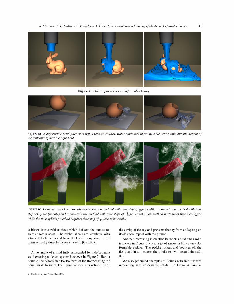
Figure 4: Paint is poured over a deformable bunny.

Figure 5: A deformable bowl filled with liquid falls on shallow water contained in an invisible water tank, hits the bottom ofthe tank and squirts the liquid out.

Figure 6: Comparisons of our simultaneous coupling method with time step of 130 sec (left), a time-splitting method with time

steps of 130 sec (middle) and a time-splitting method with time steps of 1

120 sec (right). Our method is stable at time step 130 sec

while the time splitting method requires time step of 1120 sec to be stable.

is blown into a rubber sheet which deflects the smoke to-wards another sheet. The rubber sheets are simulated withtetrahedral elements and have thickness as opposed to theinfinitesimally thin cloth sheets used in [GSLF05].

An example of a fluid fully surrounded by a deformablesolid creating a closed system is shown in Figure 2. Here aliquid-filled deformable toy bounces of the floor causing theliquid inside to swirl. The liquid conserves its volume inside

the cavity of the toy and prevents the toy from collapsing onitself upon impact with the ground.

Another interesting interaction between a fluid and a solidis shown in Figure 3 where a jet of smoke is blown on a de-formable paddle. The paddle rotates and bounces off thefloor, and in turn causes the smoke to swirl around the pad-dle.

We also generated examples of liquids with free surfacesinteracting with deformable solids. In Figure 4 paint is



poured over a bunny causing it to deform under it. Framesfrom an animation of a bowl filled with liquid falling ontoa shallow water contained in an invisible tank are shown inFigure 5. The impact causes the bowl to deform and squirtthe liquid out. Both of these examples are generated using aregular grid fluid simulator.

In Figure 6 we compare results obtained using a time-splitting method with our method of simultaneous coupling.The time-splitting method alternates between simulating thesolid, with forces exerted by the fluid pressure and simulat-ing the fluid with the boundary condition provided by thesolid. Using a time step of 1

30 the time-splitting methodquickly goes unstable while our simultaneous method re-mains stable. Only after reducing the time step to 1

120 (4×smaller) are we able to obtain a stable time-splitting solution.On a per-time step basis our method takes longer becausewe solve the larger non-symmetric linear system from Equa-tion (7), but this difference is more than compensated by thefact that we can take larger time steps. Additionally, we hadoriginally wanted to simulate a bar with less damping in or-der to get a more interesting motion of the bar, however ob-taining a stable solution for the time-splitting case requireda small enough time step to render our attempts impractical.

The collision detection and response module for our finiteelement based tetrahedral deformable solid simulator is inits early stages. Even though we respond to the collisionswith surrounding obstacles our current implementation doesnot account for self-collisions of a deformable body. Thisis apparent in our bunny example where the right ear of thebunny goes through the head and pokes through the noseof the bunny in our video. We also do not prevent inver-sion of solid tetrahedra which could lead into problems withaccuracy. Currently we are investigating methods that arerobust against element inversions such as the one proposedin [ITF04].

The main drawback of the method presented in this paperis that we need to solve a large non-symmetric linear systemthat is composed of all fluid and solid degrees of freedom inthe domain instead of solving smaller symmetric linear sys-tems for each separately. The main structure of the systemresembles a block diagonal matrix where each block repre-sents the individual solid body and fluid system. The onlyentries outside the block diagonal region are those used inthe coupling of the boundary values. Therefore the systemis still very sparse and efficient to solve with preconditionediterative methods, and by solving it our method does not in-cur an overhead large enough to offset the advantage of usinglarge time steps.

AcknowledgmentsWe thank the other members of the Berkeley Graphics Group fortheir helpful criticism and comments. This work was supported inpart by California MICRO 04-066 and 05-044, and by generous sup-port from Apple Computer, Pixar Animation Studios, Autodesk, In-tel Corporation, Sony Computer Entertainment America, and the

Alfred P. Sloan Foundation. Feldman were supported by NSF Grad-uate Fellowships.

References[BGOS06] BARGTEIL A. W., GOKTEKIN T. G., O’BRIEN J. F.,

STRAIN J. A.: A semi-Lagrangian contouring method for fluidsimulation. ACM Transactions on Graphics 25, 1 (2006).

[CMP89] COOK R. D., MALKUS D. S., PLESHA M. E.: Con-cepts and Applications of Finite Element Analysis, third ed. JohnWiley & Sons Inc., New York, 1989.

[CMT04] CARLSON M., MUCHA P. J., TURK G.: Rigid fluid:Animating the interplay between rigid bodies and fluid. In theProceedings of ACM SIGGRAPH 2004 (Aug. 2004), pp. 377–384.

[EMF02] ENRIGHT D., MARSCHNER S., FEDKIW R.: Anima-tion and rendering of complex water surfaces. In the Proceedingsof ACM SIGGRAPH 2002 (Aug. 2002), pp. 736–744.

[FF01] FOSTER N., FEDKIW R.: Practical animation of liq-uids. In the Proceedings of ACM SIGGRAPH 2001 (Aug. 2001),pp. 23–30.

[FM96] FOSTER N., METAXAS D.: Realistic animation of liq-uids. In Graphics Interface 1996 (May 1996), pp. 204–212.

[FOA03] FELDMAN B. E., O’BRIEN J. F., ARIKAN O.: Ani-mating suspended particle explosions. In Proceedings of ACMSIGGRAPH 2003 (Aug. 2003), pp. 708–715.

[FOK05] FELDMAN B. E., O’BRIEN J. F., KLINGNER B. M.:Animating gases with hybrid meshes. In Proceedings of ACMSIGGRAPH 2005 (Aug. 2005).

[FOKG05] FELDMAN B. E., O’BRIEN J. F., KLINGNER B. M.,GOKTEKIN T. G.: Fluids in deforming meshes. In ACM SIG-GRAPH/Eurographics Symposium on Computer Animation 2005(July 2005).

[FSJ01] FEDKIW R., STAM J., JENSEN H. W.: Visual simulationof smoke. In the Proceedings of ACM SIGGRAPH 2001 (Aug.2001), pp. 15–22.

[GAD03] GENEVAUX O., A H., DISCHLER J. M.: Simulatingfluid-solid interaction. In Graphics Interface (2003), pp. 31–38.

[GBO04] GOKTEKIN T. G., BARGTEIL A. W., O’BRIEN J. F.:A method for animating viscoelastic fluids. ACM Transactionson Graphics (Proc. of ACM SIGGRAPH 2004) 23, 3 (2004), 463–468.

[GSLF05] GUENDELMAN E., SELLE A., LOSASSO F., FEDKIW

R.: Coupling water and smoke to thin deformable and rigidshells. In Proceedings of ACM SIGGRAPH 2005 (Aug. 2005),pp. 457–462.

[ITF04] IRVING G., TERAN J., FEDKIW R.: Invertible finite el-ements for robust simulation of large deformation. In 2004 ACMSIGGRAPH / Eurographics Symposium on Computer Animation(July 2004), pp. 131–140.

[KFCO06] KLINGNER B. M., FELDMAN B. E., CHENTANEZ

N., O’BRIEN J. F.: Fluid animation with dynamic meshes. InProceedings of ACM SIGGRAPH 2006 (Aug. 2006).

[LGF04] LOSASSO F., GIBOU F., FEDKIW R.: Simulating waterand smoke with an octree data structure. In Proceedings of ACMSIGGRAPH 2004 (Aug. 2004), pp. 457–462.



[LL01] LI Z., LAI M.-C.: The immersed interface method forthe Navier−Stokes equations with singular forces. Journal ofComputational Physics 171 (2001), 822–842.

[MST∗04] MUELLER M., SCHIRM S., TESCHNER M., HEIDEL-BERGER B., GROSS M.: Interaction of fluids with deformablesolids. In Proceedings of Computer Animation & Social AgentsCASA’04 (July 2004), pp. 159–171.

[NFJ02] NGUYEN D., FEDKIW R., JENSEN H.: Physically basedmodeling and animation of fire. In Proceedings of ACM SIG-GRAPH 2002 (2002).

[NMK∗05] NEALAN A., MÜLLER M., KEISER R., BOXER-MANN E., CARLSON M.: Physically based deformable mod-els in computer graphics. In STAR Proceedings of Eurographics2005 (Sept. 2005), pp. 71–94.

[OH99] O’BRIEN J. F., HODGINS J. K.: Graphical modeling andanimation of brittle fracture. In Proceedings of ACM SIGGRAPH1999 (Aug. 1999), pp. 137–146.

[Pes02] PESKIN C.: The immersed boundary method. Acta Nu-merica 11 (2002), 479–517.

[Sta99] STAM J.: Stable fluids. In the Proceedings of ACM SIG-GRAPH 99 (Aug. 1999), pp. 121–128.

[TPBF87] TERZOPOULOS D., PLATT J., BARR A., FLEISCHER

K.: Elastically deformable models. International Conference onComputer Graphics and Interactive Techniques (1987), 205–214.

[YOH00] YNGVE G. D., O’BRIEN J. F., HODGINS J. K.: Ani-mating explosions. In the Proceedings of ACM SIGGRAPH 2000(July 2000), pp. 29–36.

AppendixThe time integration of Equation (3) using the general Newmarkscheme results in the following set of equations:

Man+1 + C(un+1,dn+1)+ K(dn+1)− f n+1p − f n+1

e = 0 (9)

dn+1 = dn + hun +(12−β)h2an + βh2an+1 (10)

un+1 = un +(1− γ)han + γhan+1 (11)

Choosing the integration parameters β = 12 and γ = 1, and substi-

tuting Equation (11) into Equation (10) we obtain the trapezoidalrule:

dn+1 = dn +h2(un + un+1) (12)

un+1 = un + han+1 (13)

According to Equation (13) the acceleration an+1 can be estimatedas:

an+1 =1h(un+1 −un) (14)

Substituting Equation (14) and Equation (12) into Equation (9), andassuming Rayleigh damping we obtain:

1h

M(un+1−un)+Cun+1+K(dn+h2(un + un+1))− f n+1

p − f n+1e = 0

(15)The first order approximation to the non-linear stiffness above canbe written as:

K(dn +h2(un + un+1)) = K(dn)+

h2

K′ (un + un+1) (16)

where K′ = ∂K∂d |d=dn . Substituting this into Equation (15) we obtain:

1h

M(un+1−un)+Cun+1+K(dn)+h2

K′(un+un+1)−f n+1p −f n+1

e =0

(17)Collecting the terms involving un+1 and un, and using the fact thatf n+1p = Jpn+1, we finally obtain:

(1h

M+C+h2

K′)un+1−Jpn+1 =(1h

M−h2

K′)un−K(dn)+ f n+1e

(18)which is same as Equation (4).


simultaneous coupling of fluids and deformable bodies

Documents