simultaneous cyclic scheduling and control of tubular...
TRANSCRIPT
Simultaneous Cyclic Scheduling and Control ofTubular Reactors: Parallel Production Lines
Antonio Flores-Tlacuahuac∗
Departamento de Ingenierıa y Ciencias Quımicas, Universidad Iberoamericana
Prolongacion Paseo de la Reforma 880, Mexico D.F., 01210, Mexico
Ignacio E. GrossmannDepartment of Chemical Engineering, Carnegie-Mellon University
5000 Forbes Av., Pittsburgh 15213, PA
December 20, 2010
∗Author to whom correspondence should be addressed. E-mail: [email protected], phone/fax: +52(55)59504074,http://200.13.98.241/∼antonio
1
Abstract
In this work we propose a simultaneous scheduling and control optimization formulation to ad-
dress both optimal steady-state production and dynamic product transitions in multiproduct tubular
reactors working in several parallel production lines. Because the problem involves integer and contin-
uous variables and the dynamic behavior of the underlying system the resulting optimization problem
is cast as a Mixed-Integer Dynamic Optimization (MIDO) problem. Moreover, because spatial and
temporal variations are considered when modeling the addressed systems, the dynamic systems give
rise to a system of one-dimensional partial differential equations. For solving the MIDO problems
we transform them into a mixed-integer nonlinear programs (MINLP). We use the method of lines
for spatial discretization, whereas orthogonal collocation on finite elements was used for temporal
discretization. The proposed simultaneous scheduling and control formulation is tested using three
multiproduct continuous tubular reactors featuring complex nonlinear behavior.
2
1 Introduction
We present an extension of previous work reported on the simultaneous scheduling and control (SC) of
tubular reactors in a single production line [1] to the case of parallel production lines. We refer to the
reader to previous publications of our research group [2] and others [3, 4] for a detailed description of SC
problems as well as for a recent literature review on this research topic.
Scheduling and control problems are examples of highly integrated production systems where improved
optimal solutions can be found by simultaneously solving SC problems in comparison to the case when both
problems are solved sequentially. However, the simultaneous solution of SC problems demands significant
computational effort. As the complexity of the addressed production system grows, so does the solution
of the underlying optimization problem. In previous works [2, 5] we have addressed the efficient solution
of SC problems by casting as Mixed-Integer Dynamic Optimization (MIDO) problem that upon proper
transformation can be transformed into Mixed-Integer Non-Linear Programs (MINLP).
In this work we use a previous SC formulation [1] aimed at tubular reactors in a single production line
and extend it to deal with tubular reactors in several parallel production lines. We have taken a SC
optimization formulation for several production lines in lumped systems [6] and extended it to distributed
parameters systems. We would like to highlight that the aforementioned extension is not trivial since it
involves a larger number of integer and continuous decision variables. Moreover, the nonlinear behavior
embedded in the mathematical models of the addressed systems are explicitly taken into account giving
rise to more complex and demanding MINLP problems whose solution demands the use of a decomposition
scheme for initialization as proposed in this work. The SC optimization formulation for tubular reactors in
parallel lines is illustrated trough the solution of three tubular reactors examples of increasing complexity.
2 Problem definition
Given are a number of products that are to be manufactured in a series of PFRs in a parallel production
lines arrangement. Steady-state operating conditions for manufacturing each product are also computed,
3

as well as the demand rate and price of each product and the inventory and raw materials costs. The
problem consists of the simultaneous determination of the optimal production wheel (i.e. cyclic time and
the sequence in which the products will be manufactured) as well as the transition times, production rates,
length of processing times, amounts manufactured of each product, leading to the maximization of the
economic profit and subject to meet a series of constraints representing scheduling and dynamic transition
decisions.
Similarly to work reported previously [2], in the following simultaneous scheduling and control (SSC)
formulation for parallel production plants, we assume that (1) each production line is composed of a
single plug flow tubular reactor (PFR), where desired products are manufactured, and (2) the products
follow a production wheel, meaning that all the required products are manufactured in an optimal cyclic
sequence (see Sahinidis and Grossmann [7] for a discussion on parallel line scheduling formulation). As
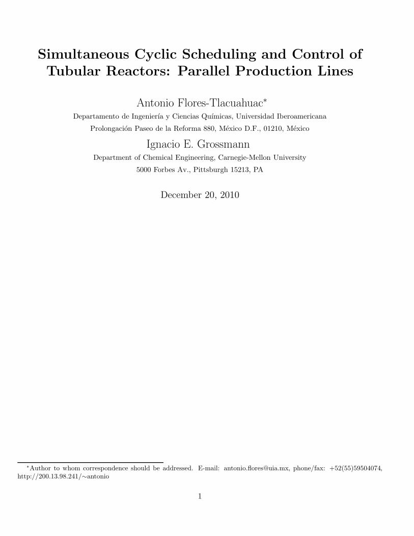
shown in Figure 1a, each production line is divided into a set of slots. We stress that the number of slots
is unknown since we do not know ahead of time how many products will be assigned in each production
line. We recall that two operations happen inside each slot: a transition period between the products
that are to be manufactured and a continuous production period. Figure 1b displays these two dynamic
generic responses conceptually. When the optimizer decides to switch to a new product, the optimization
formulation will try to develop the best dynamic transition policy featuring the minimum transition. After
the system reaches the processing conditions leading to the desired product, the system remains there until
the production specifications are met. In this work, we assume that, after a production wheel is completed,
new identical cycles are executed indefinitely. The detailed formulation of the MIDO involved is given in
the appendix.
3 MIDO solution strategy
The efficient solution of MIDO problem is a complex task. Presently, we can solve MIDO problems
mainly for small or medium size problems. However, as the number of binary variables tends to grow
so does the computational time. Moreover, the problem becomes more difficult to converge due to the
4
Slot 1 Slot 2 Slot Ns
Production Period
Transition period
Cyclic time(a)
Transition Period Production period
x
u
Sta
te, C
ontr
ol v
aria
bles
(b)
Figure 1: (a) The process consists of l parallel production lines. At each line l the cyclic time is dividedinto Ns slots. (b) When a change in the set-point of the system occurs there is a transition period followedby a continuous production period.
presence of nonlinear behavior such as multiple steady states, parametric sensitivity, oscillatory behavior,
etc. The optimization of distributed parameter systems (DPS) will only add complexity to the already
complex solution of MIDO problems because of the infinite dimensional nature of such systems. Presently
the MIDO solution of complex and large scale problems seems to be feasible only if special optimization
decomposition procedures are used [8], [9], [10], [11], [12]. In fact, the solution of MIDO problems normally
demands efficient initialization and solution procedures. Without them sometimes it is almost impossible
to compute an optimal solution.
In this work we take advantage of the structure embedded in scheduling and control problems such that a
5
solution strategy can be developed and that will allow us to compute optimal solutions of the addressed
MIDO problems. This means that the MIDO problem was decomposed into simpler parts. The solution of
the simpler parts was used to provide initial guesses to more complex versions of the MIDO problem until
the original problem to be solved was obtained. The decomposition and MIDO solution strategy involves
the following steps:
1. Solve the parallel lines scheduling problem to obtain an initial scheduling solution using guesses of
the transition times and production rates.
2. Compute steady-state processing conditions of the desired products.
3. Solve the dynamic optimization problem to obtain initial optimal transition times and production
rates.
4. Solve the entire MIDO problem for the simultaneous scheduling and control problem.
We have used the aforementioned solution strategy for computing MIDO optimal solutions with a reason-
able computational effort for all the problems addressed in the present work. We found that if a direct
solution approach is used (meaning the solution of the entire MIDO problem approached in a single step)
in most of the case studies it was impossible to compute an optimal solution. Even when a solution
could be found, an increase around 2-3 orders of magnitude in computation time was required. This is so
because very good initial values of the decision variables are normally required for the efficient solution of
dynamic optimization problems using the simultaneous approach as described in [13]. In all cases the opti-
mal solutions using either approach were the same with the computational load being the main difference
between both solution methods. For any solution method (decomposition or direct) only local solutions
were sought. The computation of global optimal solutions for the addressed MINLP problems requires
large computational times and was not addressed in the present work. Accordingly, all the simultaneous
scheduling and control problems were solved using the above solution strategy. For the numerical solution
of the MINLP problem arising from the discretization of the original MIDO problem, the SBB MINLP
solver in gams [14] was used.
6
Discretization of distributed parameter systems using finite difference techniques demands some care re-
garding the selection of both the number of discretization points and the kind of discretization equations.
For instance, it is well known that distributed parameter systems featuring convection and diffusion terms
require different discretization strategies for each one these terms [15]. Regarding the number of points
for discretization purposes we normally set this number after comparing results using different number of
discrete points. As a rule of thumb we keep reducing the number of points until from one iteration to
another the results are practically the same. Of course, at first sight, we can be tempted to use a large
number of discrete points aiming to get a small approximation errors. However, by increasing the number
of discrete points we also include the stiffness of the system. Therefore, a trade-off between approximation
error and stiffness ought to be observed. Hence, we came to the conclusion after some trials that 11 equal
sized points were enough for spatial discretization, whereas 20 finite elements and 3 internal collocation
points sufficed for time discretization. Moreover, all the problems were solved using 2 Ghz, 4 Gb computer.
4 Case studies
In this section several simultaneous scheduling and control problems taking place in tubular reactors
are addressed using the optimization formulation shown in the appendix. The examples were selected
to feature different degrees of steady-state and dynamic nonlinear behavior, such that the complexity
of solving scheduling and control problems is highlighted. We also did so hoping to justify the use of
advanced decomposition optimization techniques such as Lagrangian decomposition [8] to address the
scheduling and control of more complex reaction system such as polymerization reaction systems. We
stress that for all the case studies all the parallel lines are equipped with identical PFRs. Moreover, when
discussing results we define a productivity term for each product in a given production line as the ratio of
the amount manufactured of such product in the production line divided by the corresponding cyclic time
of the production line.
7
Isothermal tubular reactor
To test the proposed SSC optimization formulation we have selected as the first case study a problem
that is relatively easy to optimize but that will allow us to tackle more complex systems. The system in
question consists of an isothermal plug flow reactor with both convective and diffusive mass transfer and
where the 2X → Y second order reaction takes place. The distributed model is given as follows:
∂C
∂t= D
∂2C
∂x2− v
∂C
∂x−KC2 (1)
subject to the following initial,
C(x, 0) = Cf (2)
and boundary conditions,
@ x = 0 C = Cf +D
v
∂C
∂x(3)
@ x = L∂C
∂x= 0 (4)
where C stands for the concentration of the X component, x is the longitudinal coordinate, t is the time,
D is the mass diffusivity and v is the linear velocity, K is the reaction constant, Cf is the feed stream
composition of reactant X and L is the reactor length. To improve the chances of finding an optimal
solution the model is scaled as follows:
C′
=C
Cf
, x′
=x
L, θ =
tv
L
Hence, in terms of the dimensionless variables, the scaled model reads as follows,
∂C′
∂θ=
1
PeM
∂2C′
∂x′2
−∂C
′
∂x′−
α
PeMC
′2 (5)
8
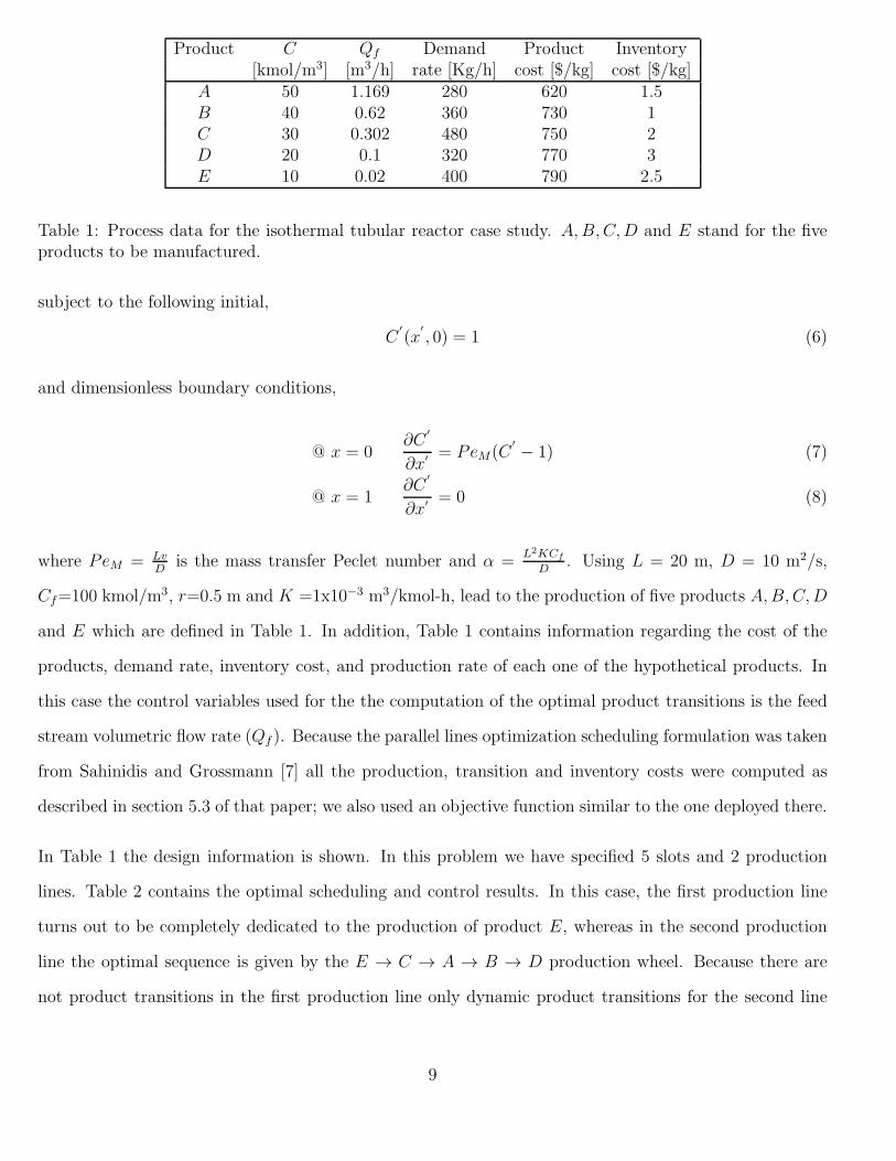
Product C Qf Demand Product Inventory[kmol/m3] [m3/h] rate [Kg/h] cost [$/kg] cost [$/kg]
A 50 1.169 280 620 1.5B 40 0.62 360 730 1C 30 0.302 480 750 2D 20 0.1 320 770 3E 10 0.02 400 790 2.5
Table 1: Process data for the isothermal tubular reactor case study. A,B,C,D and E stand for the fiveproducts to be manufactured.
subject to the following initial,
C′
(x′
, 0) = 1 (6)
and dimensionless boundary conditions,
@ x = 0∂C
′
∂x′= PeM(C
′
− 1) (7)
@ x = 1∂C
′
∂x′= 0 (8)
where PeM = LvD
is the mass transfer Peclet number and α =L2KCf
D. Using L = 20 m, D = 10 m2/s,
Cf=100 kmol/m3, r=0.5 m and K =1x10⁻³ m3/kmol-h, lead to the production of five products A,B,C,D
and E which are defined in Table 1. In addition, Table 1 contains information regarding the cost of the
products, demand rate, inventory cost, and production rate of each one of the hypothetical products. In
this case the control variables used for the the computation of the optimal product transitions is the feed
stream volumetric flow rate (Qf ). Because the parallel lines optimization scheduling formulation was taken
from Sahinidis and Grossmann [7] all the production, transition and inventory costs were computed as
described in section 5.3 of that paper; we also used an objective function similar to the one deployed there.
In Table 1 the design information is shown. In this problem we have specified 5 slots and 2 production
lines. Table 2 contains the optimal scheduling and control results. In this case, the first production line
turns out to be completely dedicated to the production of product E, whereas in the second production
line the optimal sequence is given by the E → C → A → B → D production wheel. Because there are
not product transitions in the first production line only dynamic product transitions for the second line
9
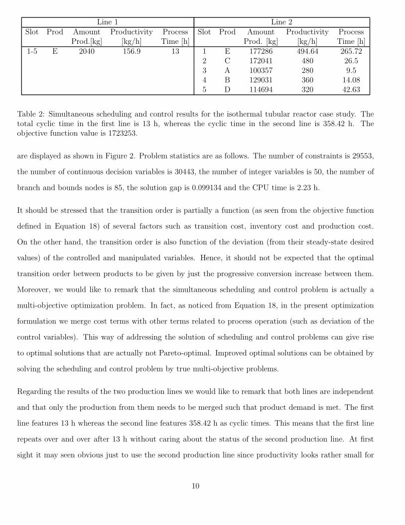
Line 1 Line 2Slot Prod Amount Productivity Process Slot Prod Amount Productivity Process
Prod.[kg] [kg/h] Time [h] Prod. [kg] [kg/h] Time [h]1-5 E 2040 156.9 13 1 E 177286 494.64 265.72
2 C 172041 480 26.53 A 100357 280 9.54 B 129031 360 14.085 D 114694 320 42.63
Table 2: Simultaneous scheduling and control results for the isothermal tubular reactor case study. Thetotal cyclic time in the first line is 13 h, whereas the cyclic time in the second line is 358.42 h. Theobjective function value is 1723253.
are displayed as shown in Figure 2. Problem statistics are as follows. The number of constraints is 29553,
the number of continuous decision variables is 30443, the number of integer variables is 50, the number of
branch and bounds nodes is 85, the solution gap is 0.099134 and the CPU time is 2.23 h.
It should be stressed that the transition order is partially a function (as seen from the objective function
defined in Equation 18) of several factors such as transition cost, inventory cost and production cost.
On the other hand, the transition order is also function of the deviation (from their steady-state desired
values) of the controlled and manipulated variables. Hence, it should not be expected that the optimal
transition order between products to be given by just the progressive conversion increase between them.
Moreover, we would like to remark that the simultaneous scheduling and control problem is actually a
multi-objective optimization problem. In fact, as noticed from Equation 18, in the present optimization
formulation we merge cost terms with other terms related to process operation (such as deviation of the
control variables). This way of addressing the solution of scheduling and control problems can give rise
to optimal solutions that are actually not Pareto-optimal. Improved optimal solutions can be obtained by
solving the scheduling and control problem by true multi-objective problems.
Regarding the results of the two production lines we would like to remark that both lines are independent
and that only the production from them needs to be merged such that product demand is met. The first
line features 13 h whereas the second line features 358.42 h as cyclic times. This means that the first line
repeats over and over after 13 h without caring about the status of the second production line. At first
sight it may seen obvious just to use the second production line since productivity looks rather small for
10
0 0.5 1 1.5 2 2.5 30
10
20
30
40
50
Co
nce
ntr
atio
n [km
ol/m
3]
Time [h]
Second Line
ECABD
0 0.5 1 1.5 2 2.5 30
0.2
0.4
0.6
0.8
1
1.2
1.4
Fe
ed
str
ea
m V
olu
me
tric
Flo
wra
te [m
3/h
]
Time [h]
ECABD
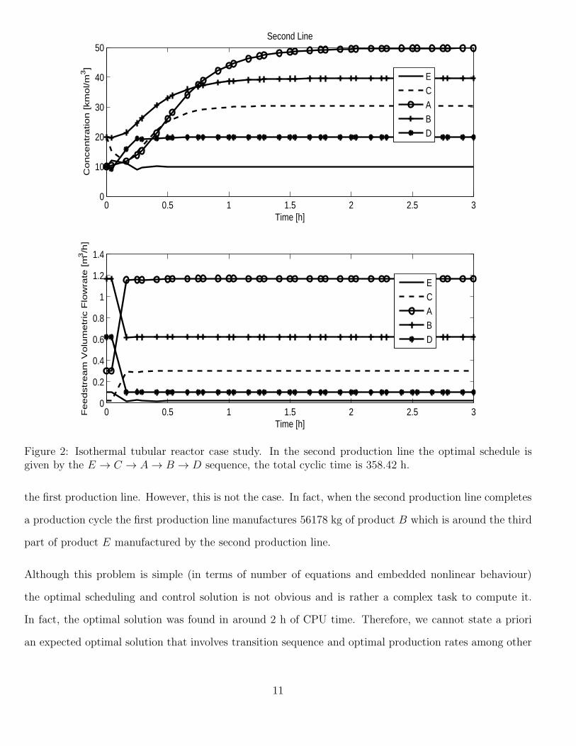
Figure 2: Isothermal tubular reactor case study. In the second production line the optimal schedule isgiven by the E → C → A → B → D sequence, the total cyclic time is 358.42 h.
the first production line. However, this is not the case. In fact, when the second production line completes
a production cycle the first production line manufactures 56178 kg of product B which is around the third
part of product E manufactured by the second production line.
Although this problem is simple (in terms of number of equations and embedded nonlinear behaviour)
the optimal scheduling and control solution is not obvious and is rather a complex task to compute it.
In fact, the optimal solution was found in around 2 h of CPU time. Therefore, we cannot state a priori
an expected optimal solution that involves transition sequence and optimal production rates among other
11
decision variables. Because of the size and complexity in dealing with the optimal solution of MINLPs
only local optimal solutions were sought.
Non-isothermal adiabatic tubular reactor
The second example refers to an irreversible first order reaction X → Y that takes place in an non-
isothermal plug flow reactor whose one-dimensional dynamic model reads as follows [16]:
∂C
∂t= −
∂C
∂z+R(C, T ) (9)
∂T
∂t= −
∂T
∂z−R(C, T )− U(Tw − T ) (10)
R(C, T ) = −1011Ce−75/t (11)
subject to the following initial,
C(z, 0) = Cf (12)
T (z, 0) = Tf (13)
and boundary conditions,
@z = 0 C = Cf +∂C∂z
(14)
@z = 0 T = Tf +∂T∂z
(15)
where C stands for the dimensionless concentration of component X , T is the dimensionless temperature,
z is the dimensionless axial coordinate, U is the dimensionless heat transfer coefficient and Tw is the di-
mensionless reactor wall temperature. Moreover, Cf = 0.85 is the dimensionless feed stream concentration
of reactant X and Tf = 2.713 is the dimensionless feed stream temperature. For modeling this system
we have assumed that mass and heat transport occur only along the axial reactor direction and that the
diffusive effects can be neglected.
12
2.62 2.64 2.66 2.68 2.7 2.72 2.74 2.76 2.78 2.8−0.1
0
0.1
0.2
0.3
0.4
0.5
0.6
0.7
0.8
0.9
Tf
C
A
B
C
(a)
2.62 2.64 2.66 2.68 2.7 2.72 2.74 2.76 2.78 2.82.6
2.8
3
3.2
3.4
3.6
3.8
4
Tf
T
A
B
C
(b)
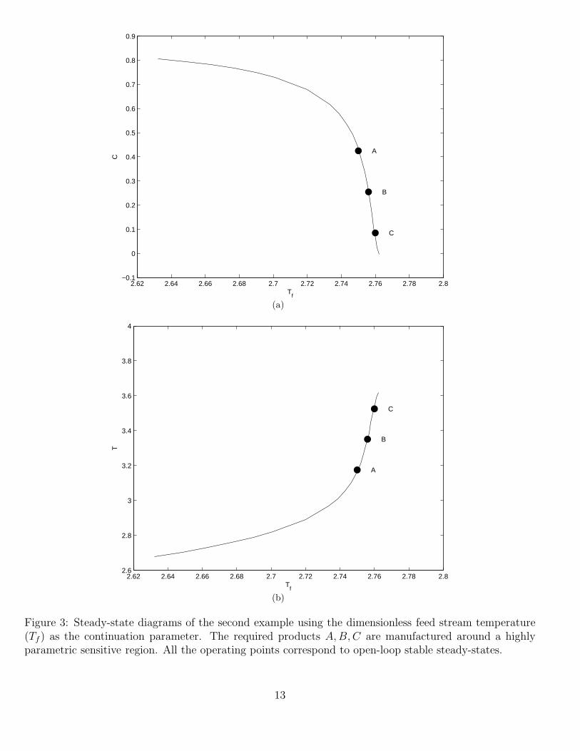
Figure 3: Steady-state diagrams of the second example using the dimensionless feed stream temperature(Tf ) as the continuation parameter. The required products A,B,C are manufactured around a highlyparametric sensitive region. All the operating points correspond to open-loop stable steady-states.
13
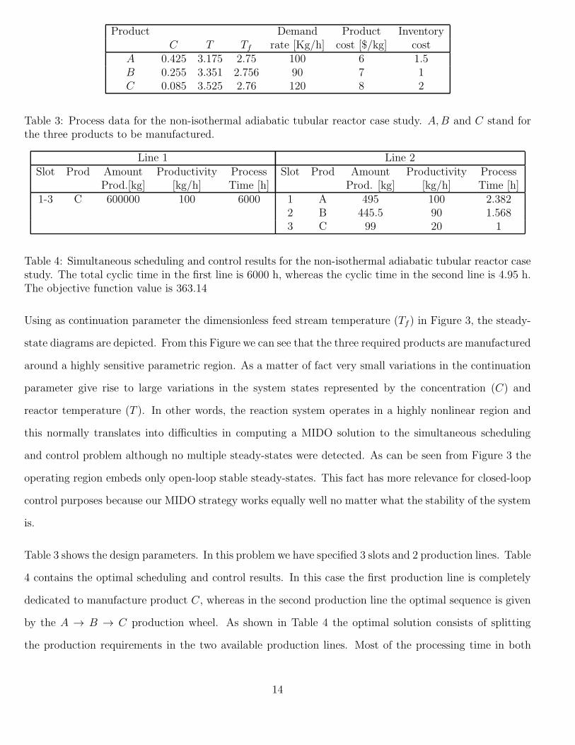
Product Demand Product InventoryC T Tf rate [Kg/h] cost [$/kg] cost
A 0.425 3.175 2.75 100 6 1.5B 0.255 3.351 2.756 90 7 1C 0.085 3.525 2.76 120 8 2
Table 3: Process data for the non-isothermal adiabatic tubular reactor case study. A,B and C stand forthe three products to be manufactured.
Line 1 Line 2Slot Prod Amount Productivity Process Slot Prod Amount Productivity Process
Prod.[kg] [kg/h] Time [h] Prod. [kg] [kg/h] Time [h]1-3 C 600000 100 6000 1 A 495 100 2.382
2 B 445.5 90 1.5683 C 99 20 1
Table 4: Simultaneous scheduling and control results for the non-isothermal adiabatic tubular reactor casestudy. The total cyclic time in the first line is 6000 h, whereas the cyclic time in the second line is 4.95 h.The objective function value is 363.14
Using as continuation parameter the dimensionless feed stream temperature (Tf ) in Figure 3, the steady-
state diagrams are depicted. From this Figure we can see that the three required products are manufactured
around a highly sensitive parametric region. As a matter of fact very small variations in the continuation
parameter give rise to large variations in the system states represented by the concentration (C) and
reactor temperature (T ). In other words, the reaction system operates in a highly nonlinear region and
this normally translates into difficulties in computing a MIDO solution to the simultaneous scheduling
and control problem although no multiple steady-states were detected. As can be seen from Figure 3 the
operating region embeds only open-loop stable steady-states. This fact has more relevance for closed-loop
control purposes because our MIDO strategy works equally well no matter what the stability of the system
is.
Table 3 shows the design parameters. In this problem we have specified 3 slots and 2 production lines. Table
4 contains the optimal scheduling and control results. In this case the first production line is completely
dedicated to manufacture product C, whereas in the second production line the optimal sequence is given
by the A → B → C production wheel. As shown in Table 4 the optimal solution consists of splitting
the production requirements in the two available production lines. Most of the processing time in both
14
production lines is dedicated to manufacture product C. Because the cost of the inventories is relatively
low, the optimal solution consists in manufacturing as much as possible of each one of the products. In fact,
the demand rate for each product is completely fullfiled and no product is overproduced. The objective
function value is $ 363.14. Regarding the optimal dynamic transition responses, because only one product
(C) is manufactured in the first line actually no product transitions take place in this line and so no
dynamic transitions are shown. However, optimal dynamic transitions occur for the second line and they
are shown in Figure 4. It is worth to mention that when changing the value of the controlled variable in a
step-like form between any couple of the products, the open-loop transition times turn out to be extremely
small. This is so because, as seen in Figure 3, the distributed parameter system operates around a highly
sensitivity region: very small changes in the value of Tf cause a transition from an initial to a final product.
In practical terms, we can consider that the tubular reactor operates in a quasi steady-state pattern. This
explains the shape of the optimal dynamic response displayed in Figure 4. Hence, we expected, as it
was the case, short optimal transition times between the steady-state processing conditions. Therefore,
when preparing Figure 4 the abscissa coordinate (i.e. processing time) was divided by the maximum
observed transition time among all optimal transition curves. A similar procedure was deployed to scale
the processing time of the third case study. From Figures 3(a) and 3(b) it is clear that the same kind of
process sensitivity is exhibited either in terms of concentration or temperature. For this reason we decided
not to include the reactor temperature response curves. As a matter of fact, the reactor temperature
curves are very similar (in shape) to the reactor concentration response curves (see top part of Figure 4):
the optimal response curve features fast transitions from one steady-state to another. Problem statistics
are as follows. The number of constraints is 50928, the number of continuous decision variables is 51468,
the number of integer variables is 18 and the CPU time is 2.50 min using GAMS/SBB.
15
0 0.1 0.2 0.3 0.4 0.5 0.6 0.7 0.8 0.9 10
0.1
0.2
0.3
0.4
0.5
Co
nce
ntr
atio
n [km
ol/m
3]
Time []
Second Line
ABC
0 0.1 0.2 0.3 0.4 0.5 0.6 0.7 0.8 0.9 12.748
2.75
2.752
2.754
2.756
2.758
2.76
2.762
Fe
ed
str
ea
m T
em
pe
ratu
re []
Time []
ABC
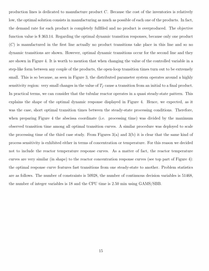
Figure 4: Non-isothermal adiabatic tubular reactor case study. The second line optimal production se-quence is A → B → C. The cyclic time is 4.95 h.
Non-isothermal adiabatic tubular reactor with recycle and mixing tank
The third example is a variation of the second case study where no recycle was allowed [16]. As depicted
in Figure 5, the modification consists in introducing a recycle stream and in mixing the main feed stream
with the recycle stream, the resulting stream is fed to the tubular reactor.
The dynamic mathematical model describing this case study is the same represented by Equations 9-
15. However, the concentration (Co) and temperature (To) of the main feed stream are described by the
16
C fT
f
C o
To
R
1−ReC
Te
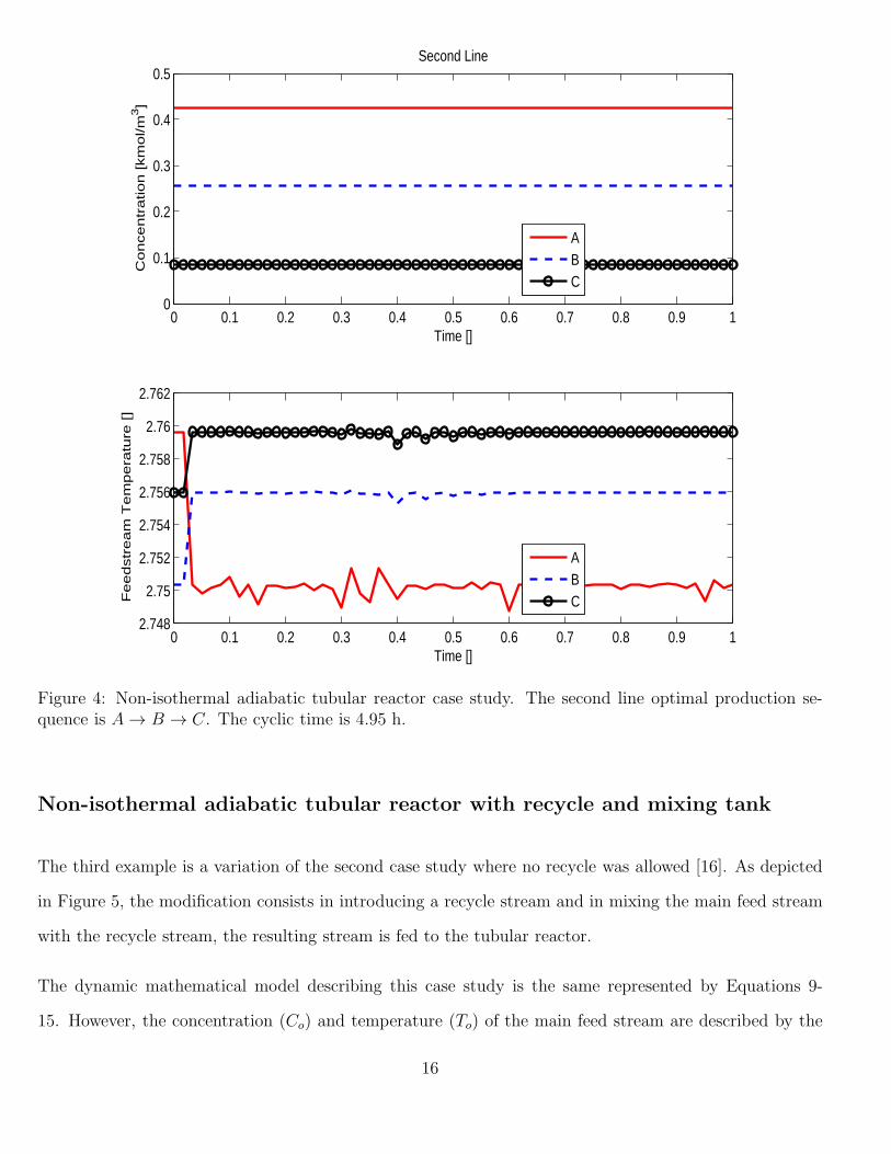
Figure 5: Nonisothermal, adiabatic plug flow tubular reactor with recycle stream and mixing tank.
following set of algebraic equations:
Co = (1−R)Cf +RCe (16)
To = (1−R)Tf +RTe (17)
where R = 0.5 is the recycle fraction, Ce, Te are the outlet dimensionless concentration and temperature,
respectively. Moreover, in this case study the values of the dimensionless feed stream concentration Cf
and temperature Tf are 1 and 2.3, respectively.
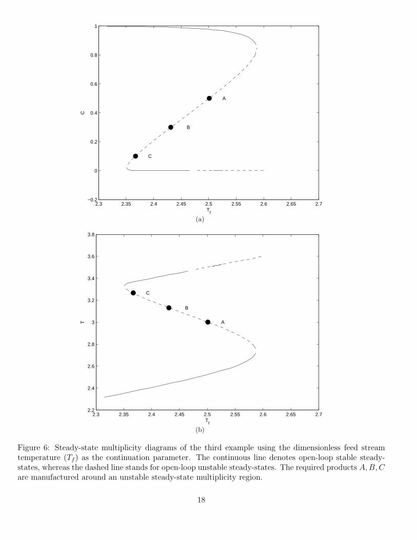
Figure 6 depicts the steady-state multiplicity diagram of the addressed system using the dimensionless feed
stream temperature (Tf) as continuation parameter. As noted, the three required products A,B,C are
manufactured around an open-loop steady-state unstable operating region where up to three steady-states
were found. The presence of multiple steady-state solutions might represent a computational difficulty for
computing a MIDO solution to the present case study. However, we do not expect additional computational
problems because of the unstable nature of the steady-states. This desired feature of our MIDO approach
has to do with using the simultaneous approach for solving dynamic optimization problems [13].
17
2.3 2.35 2.4 2.45 2.5 2.55 2.6 2.65 2.7−0.2
0
0.2
0.4
0.6
0.8
1
Tf
C
A
B
C
(a)
2.3 2.35 2.4 2.45 2.5 2.55 2.6 2.65 2.72.2
2.4
2.6
2.8
3
3.2
3.4
3.6
3.8
Tf
T A
B
C
(b)
Figure 6: Steady-state multiplicity diagrams of the third example using the dimensionless feed streamtemperature (Tf) as the continuation parameter. The continuous line denotes open-loop stable steady-states, whereas the dashed line stands for open-loop unstable steady-states. The required products A,B,C
are manufactured around an unstable steady-state multiplicity region.
18
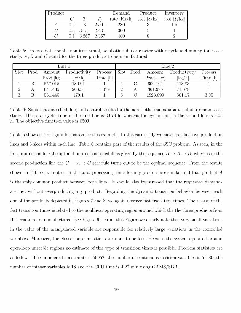
Product Demand Product InventoryC T Tf rate [Kg/h] cost [$/kg] cost [$/kg]
A 0.5 3 2.501 280 3 1.5B 0.3 3.131 2.431 360 5 1C 0.1 3.267 2.367 480 8 2
Table 5: Process data for the non-isothermal, adiabatic tubular reactor with recycle and mixing tank casestudy. A,B and C stand for the three products to be manufactured.
Line 1 Line 2Slot Prod Amount Productivity Process Slot Prod Amount Productivity Process
Prod.[kg] [kg/h] Time [h] Prod. [kg] [kg/h] Time [h]1 B 557.015 180.91 1 1 C 600.101 118.83 12 A 641.435 208.33 1.079 2 A 361.975 71.678 13 B 551.445 179.1 1 3 C 1823.899 361.17 3.05
Table 6: Simultaneous scheduling and control results for the non-isothermal adiabatic tubular reactor casestudy. The total cyclic time in the first line is 3.079 h, whereas the cyclic time in the second line is 5.05h. The objective function value is 6503.
Table 5 shows the design information for this example. In this case study we have specified two production
lines and 3 slots within each line. Table 6 contains part of the results of the SSC problem. As seen, in the
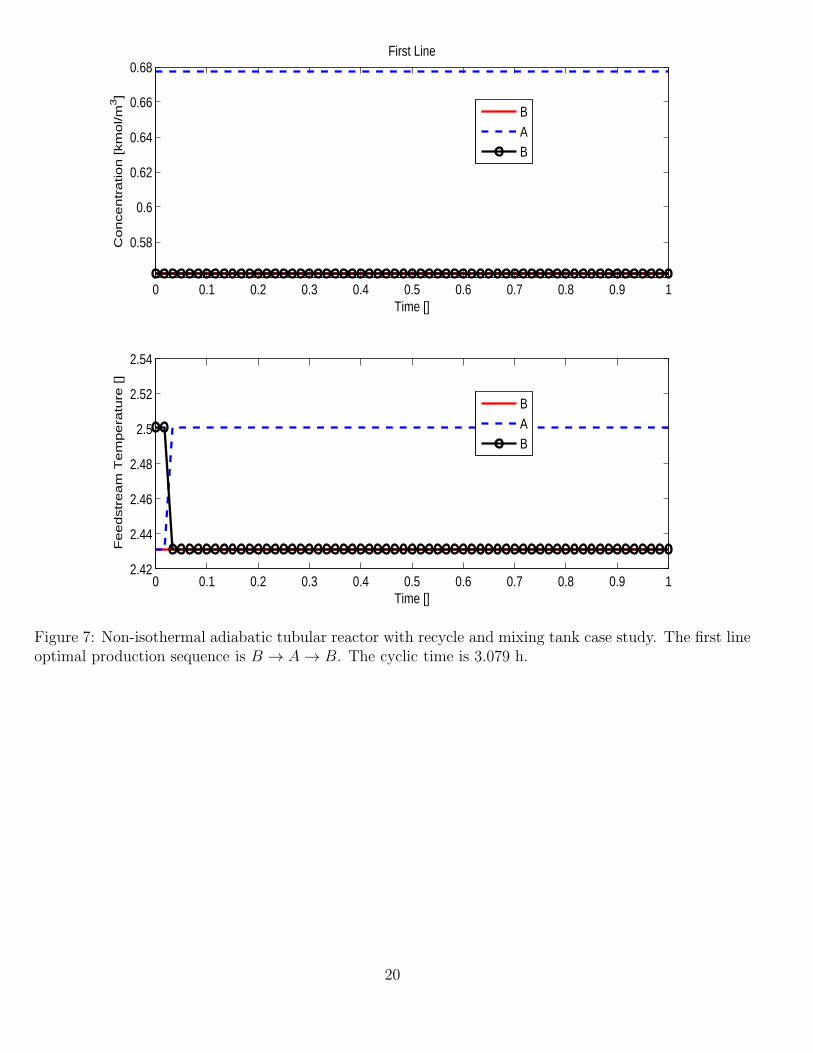
first production line the optimal production schedule is given by the sequence B → A → B, whereas in the
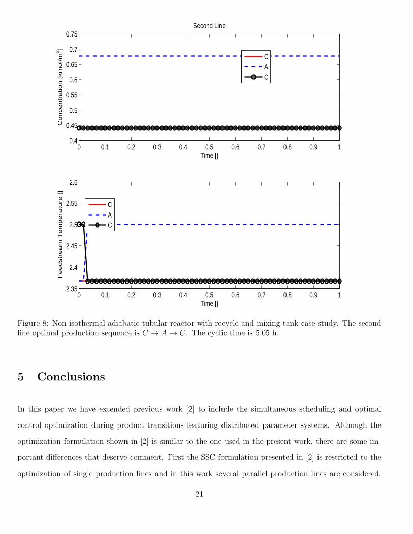
second production line the C → A → C schedule turns out to be the optimal sequence. From the results
shown in Table 6 we note that the total processing times for any product are similar and that product A
is the only common product between both lines. It should also bw stressed that the requested demands
are met without overproducing any product. Regarding the dynamic transition behavior between each
one of the products depicted in Figures 7 and 8, we again observe fast transition times. The reason of the
fast transition times is related to the nonlinear operating region around which the the three products from
this reactors are manufactured (see Figure 6). From this Figure we clearly note that very small variations
in the value of the manipulated variable are responsible for relatively large variations in the controlled
variables. Moreover, the closed-loop transitions turn out to be fast. Because the system operated around
open-loop unstable regions no estimate of this type of transition times is possible. Problem statistics are
as follows. The number of constraints is 50952, the number of continuous decision variables is 51480, the
number of integer variables is 18 and the CPU time is 4.20 min using GAMS/SBB.
19
0 0.1 0.2 0.3 0.4 0.5 0.6 0.7 0.8 0.9 1
0.58
0.6
0.62
0.64
0.66
0.68First Line
Co
nce
ntr
atio
n [
km
ol/m
3]
Time []
BAB
0 0.1 0.2 0.3 0.4 0.5 0.6 0.7 0.8 0.9 12.42
2.44
2.46
2.48
2.5
2.52
2.54
Fe
ed
str
ea
m T
em
pe
ratu
re [
]
Time []
BAB
Figure 7: Non-isothermal adiabatic tubular reactor with recycle and mixing tank case study. The first lineoptimal production sequence is B → A → B. The cyclic time is 3.079 h.
20
0 0.1 0.2 0.3 0.4 0.5 0.6 0.7 0.8 0.9 10.4
0.45
0.5
0.55
0.6
0.65
0.7
0.75
Co
nce
ntr
atio
n [
km
ol/m
3]
Time []
Second Line
CAC
0 0.1 0.2 0.3 0.4 0.5 0.6 0.7 0.8 0.9 12.35
2.4
2.45
2.5
2.55
2.6
Fe
ed
str
ea
m T
em
pe
ratu
re [
]
Time []
CAC
Figure 8: Non-isothermal adiabatic tubular reactor with recycle and mixing tank case study. The secondline optimal production sequence is C → A → C. The cyclic time is 5.05 h.
5 Conclusions
In this paper we have extended previous work [2] to include the simultaneous scheduling and optimal
control optimization during product transitions featuring distributed parameter systems. Although the
optimization formulation shown in [2] is similar to the one used in the present work, there are some im-
portant differences that deserve comment. First the SSC formulation presented in [2] is restricted to the
optimization of single production lines and in this work several parallel production lines are considered.
21

Second, such an optimization formulation assumes that the system dynamics is represented in terms of
lumped parameters systems. We have taken the scheduling optimization formulation from Sahinidis and
Grossmann [7]. However, we found that it is a no trivial task to merge it with an optimal control formula-
tion to get the SSC formulation. Regarding the system dynamics, in the present work we have addressed
the optimal control of distributed parameters systems. Intuitively, one would expect that the optimization
of distributed parameters systems to be harder than the corresponding optimization of lumped parame-
ters systems. This is so because discretized distributed parameters system give rise to a set of lumped
systems. As the dimensionality of the distributed system increases so does the complexity of solving these
kind of optimization problems. The dynamic and static optimization of distributed systems is presently
a challenging research area. Moreover, as far as we know the SSC optimization of distributed parameters
systems has not been reported in the open literature. In summary, the proposed SSC optimization formu-
lation for distributed systems operating in parallel lines has allowed us to tackle some practical problems
and compute local optimal solutions in reasonable computational time.
22
Appendix
Simultaneous Scheduling and Control Parallel Lines Optimization Formula-
tion
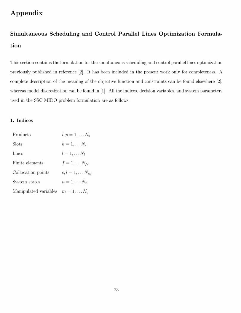
This section contains the formulation for the simultaneous scheduling and control parallel lines optimization
previously published in reference [2]. It has been included in the present work only for completeness. A
complete description of the meaning of the objective function and constraints can be found elsewhere [2],
whereas model discretization can be found in [1]. All the indices, decision variables, and system parameters
used in the SSC MIDO problem formulation are as follows.
1. Indices
Products i, p = 1, . . . Np
Slots k = 1, . . . Ns
Lines l = 1, . . .Nl
Finite elements f = 1, . . . Nfe
Collocation points c, l = 1, . . . Ncp
System states n = 1, . . .Nx
Manipulated variables m = 1, . . .Nu
23
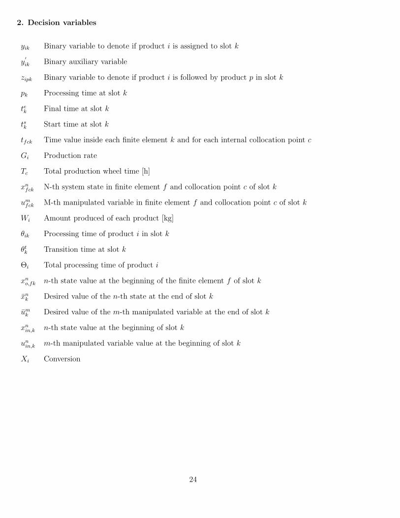
2. Decision variables
yik Binary variable to denote if product i is assigned to slot k
y′
ik Binary auxiliary variable
zipk Binary variable to denote if product i is followed by product p in slot k
pk Processing time at slot k
tek Final time at slot k
tsk Start time at slot k
tfck Time value inside each finite element k and for each internal collocation point c
Gi Production rate
Tc Total production wheel time [h]
xnfck N-th system state in finite element f and collocation point c of slot k
umfck M-th manipulated variable in finite element f and collocation point c of slot k
Wi Amount produced of each product [kg]
θik Processing time of product i in slot k
θtk Transition time at slot k
Θi Total processing time of product i
xno,fk n-th state value at the beginning of the finite element f of slot k
xnk Desired value of the n-th state at the end of slot k
umk Desired value of the m-th manipulated variable at the end of slot k
xnin,k n-th state value at the beginning of slot k
unin,k m-th manipulated variable value at the beginning of slot k
Xi Conversion
24

3. Parameters
Np Number of products
Ns Number of slots
Nl Number of lines
Nfe Number of finite elements
Ncp Number of collocation points
Nx Number of system states
Nu Number of manipulated variables
Di Demand rate [kg/h]
Cpi Price of products [$/kg]
Csi Cost of inventory [$]
Cr Cost of raw material [$]
hfk Length of finite element f in slot k
ΩNcp,NcpMatrix of Radau quadrature weights
θmax Upper bound on processing time
ttip Estimated value of the transition time between product i and p
xnss,i n-th state steady value of product i
umss,i m-th manipulated variable value of product i
F o Feed stream volumetric flow rate
Xi Conversion degree
xnmin, x
nmax Minimum and maximum value of the state xn
ummin, u
mmax Minimum and maximum value of the manipulated variable um
γNcpRoots of the Lagrange orthogonal polynomial
Objective Function
min φ =∑
i
∑
k
∑
l
cpil
t′
ikl
Tcl+∑
i
∑
j
∑
k
∑
l
ctijlZijkl
Tcl+∑
i
∑
k
∑
l
ciilWikl
+ω∑
i
δi + αx
∫ tf
0
(x− xs)2dt+ αu
∫ tf
0
(u− us)2dt (18)
25
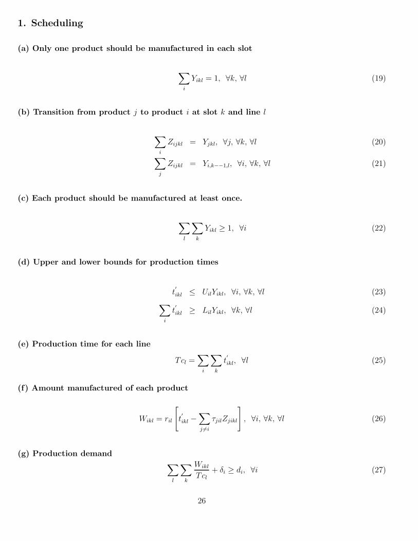
1. Scheduling
(a) Only one product should be manufactured in each slot
∑
i
Yikl = 1, ∀k, ∀l (19)
(b) Transition from product j to product i at slot k and line l
∑
i
Zijkl = Yjkl, ∀j, ∀k, ∀l (20)
∑
j
Zijkl = Yi,k−−1,l, ∀i, ∀k, ∀l (21)
(c) Each product should be manufactured at least once.
∑
l
∑
k
Yikl ≥ 1, ∀i (22)
(d) Upper and lower bounds for production times
t′
ikl ≤ UilYikl, ∀i, ∀k, ∀l (23)
∑
i
t′
ikl ≥ LilYikl, ∀k, ∀l (24)
(e) Production time for each line
Tcl =∑
i
∑
k
t′
ikl, ∀l (25)
(f) Amount manufactured of each product
Wikl = ril
[
t′
ikl −∑
j 6=i
τjilZjikl
]
, ∀i, ∀k, ∀l (26)
(g) Production demand∑
l
∑
k
Wikl
Tcl+ δi ≥ di, ∀i (27)
26
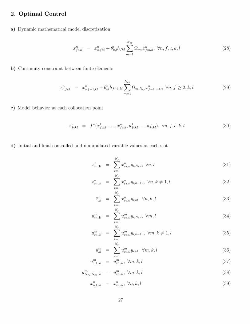
2. Optimal Control
a) Dynamic mathematical model discretization
xnfckl = xn
o,fkl + θtk,lhfkl
Ncp∑
m=1
Ωmcxnfmkl, ∀n, f, c, k, l (28)
b) Continuity constraint between finite elements
xno,fkl = xn
o,f−1,kl + θtklhf−1,kl
Ncp∑
m=1
Ωm,Ncpxnf−1,mkl, ∀n, f ≥ 2, k, l (29)
c) Model behavior at each collocation point
xnfckl = fn(x1
fckl, . . . , xnfckl, u
1
fckl, . . . umfckl), ∀n, f, c, k, l (30)
d) Initial and final controlled and manipulated variable values at each slot
xnin,1l =
Np∑
i=1
xnss,ilyi,Ns,l, ∀n, l (31)
xnin,kl =
Np∑
i=1
xnss,ilyi,k−1,l, ∀n, k 6= 1, l (32)
xnkl =
Np∑
i=1
xnss,ilyi,kl, ∀n, k, l (33)
umin,1l =
Np∑
i=1
umss,ilyi,Ns,l, ∀m, l (34)
umin,kl =
Np∑
i=1
umss,ilyi,k−1,l, ∀m, k 6= 1, l (35)
umkl =
Np∑
i=1
umss,ilyi,kl, ∀m, k, l (36)
um1,1,kl = um
in,kl, ∀m, k, l (37)
umNfe,Ncp,kl = um
in,kl, ∀m, k, l (38)
xno,1,kl = xn
in,kl, ∀n, k, l (39)
27

e) Lower and upper bounds of the decision variables
xnmin ≤ xn
fckl ≤ xnmax, ∀n, f, c, k, l (40a)
ummin ≤ um
fckl ≤ ummax, ∀m, f, c, k, l (40b)
28
References
[1] A. Flores-Tlacuahuac and I.E. Grossmann. Simultaneous cyclic scheduling and control of tubular reac-
tors: Single production lines. Accepted for publication: Ind. Eng. Chem. Res., doi:10.1021/ie1008629.
[2] A. Flores-Tlacuahuac and I.E. Grossmann. Simultaneous Cyclic Scheduling and Control of a Multi-
product CSTR. Ind. Eng. Chem. Res., 45(20):6175–6189, 2006.
[3] A. Prata, J. Oldenburg, A. Kroll, and W. Marquardt. Integrated scheduling and dynamic optimization
of grade transitions for a continuous polymerization reactor. Comput. Chem. Eng., 32(3):463–476,
2008.
[4] I. Harjunkoski, R. Nystrom, and A. Horch. Integration of Scheduling and Control: Theory or Practice?
Comput. Chem. Eng., 33(12):1909–1918, 2009.
[5] S. Terrazas-Moreno, A. Flores-Tlacuauhuac, and I.E. Grossmann. Simultaneous scheduling and con-
trol in polymerization reactors. AIChE J., 53(9), 2007.
[6] A. Flores-Tlacuahuac and I.E. Grossmann. Simultaneous scheduling and control of multiproduct
continuous parallel lines. Ind. Eng. Chem. Res., doi:10.1021/ie100024p, 2010.
[7] N. Sahinidis and I.E. Grossmann. MINLP Model for Cyclic Multiproduct Scheduling on Continuous
Parallel Lines. Comput. Chem. Eng., 15(2):85–103, 1991.
[8] M. Guinard and S.Kim. Lagrangean Decomposition: A model yielding Stronger Lagrangean Bounds.
Mathematical Programming, 39:215–228, 1987.
[9] M.L Fisher. The Lagrangian Relaxation Method for Solving Integer Programming Problems. Man-
agament Science, 27(1):2–18, 1981.
[10] A.M. Geoffrion. Lagrangean Relaxation for Integer Programming. Mathematical Programming Study,
2:82–114, 1974.
[11] M.Guignard. Lagrangean relaxation: A short course. J.OR:Special Issue Francoro, 35:3, 1995.
29
[12] S.Vasantharajan K.Edwards S.A. van den Heever, I.E. Grossmann. A Lagrangean Decomposition
Heuristic for the Design and Planning of Offshore Hydrocarbon Field Infrastructure with Complex
Economic Objectives. Ind. Eng. Chem. Res., 40:2857–2875, 2001.
[13] L.T. Biegler. An overview of simultaneous strategies for dynamic optimization. Chemical Engineering
and Processing, 46(11):1043–1053, 2007.
[14] A. Brooke, D. Kendrick, Meeraus, and R. A. Raman. GAMS: A User’s Guide. GAMS Development
Corporation, 1998, http://www.gams.com.
[15] W. E. Schiesser. The Numerical Method of Lines. Integration of Partial Differential Equations. Aca-
demic Press, Inc., 1991.
[16] G. Pareja and M.J Reilly. Dynamic Effects of Recycle Elements in Tubular Reactor Systems. Ind.
Eng. Chem. Fund., 8(3):442–448, 1969.
30