Simultaneous Planning and Scheduling of Single-Stage

Multiproduct Continuous Plants with Parallel Lines

Muge Erdirik-Dogan, Ignacio E. Grossmann∗

July 18, 2007

Department of Chemical Engineering, Carnegie Mellon University, Pittsburgh, Pennsylvania 15213

Key words: Planning; Scheduling; Multi-product continuous plants; MILP; Slot based formulation

Abstract

In this paper we present a multi-period mixed integer linear programming model for the simultaneous

planning and scheduling of single stage multi-product continuous plants with parallel units. While

e�ective for short time horizons, the proposed scheduling model becomes computationally expensive to

solve for long time horizons. In order to address this problem, we propose a bi-level decomposition

algorithm in which the original problem is decomposed into an upper level planning and a lower level

scheduling problem. For the representation of the upper level, we propose an MILP model which is

based on a relaxation of the original model, but accounts for the e�ects of scheduling by incorporating

sequencing constraints, which results in very tight upper bounds. In the lower level the simultaneous

planning and scheduling model is solved for a subset of products predicted by the upper level. These

sub-problems are solved iteratively until the upper and lower bounds converge. A number of examples

are presented that show that the planning model can often obtain the optimal schedule in one single

iteration.

1 Introduction

Despite the importance of the short-term scheduling of multi-product facilities involving continuous processes,

relatively few articles have been published in this area. Sahinidis and Grossmann [1991] considered the

problem of cyclic scheduling of multi-product plants for single stage plants with parallel units. This work

was extended by Pinto and Grossmann [1994] who considered the case of multi-stage continuous plants

with one unit per stage and with intermediate storage. Alle et al. [2004] extended this work to include

cleaning considerations. Jain and Grossmann [1998] addressed the scheduling of multiple feeds on parallel

continuous units where process performance models are also incorporated. Mendez and Cerda [2002] studied

resource constrained multi-product plants involving parallel mixers operating in a continuous mode. Even

fewer papers have appeared to address the short term scheduling of re�nery operations. Examples include

the works by Lee et al. [1996] and by Shah [1996] who addressed the problem of crude-oil unloading with

inventory control using MILP models. Another example is the work of Jia and Ierapetritou [2004] who

addressed this problem with an MINLP model.

∗Corresponding author. Tel:+1 412 268 3642; fax: +1 412 268 7139; E-mail address: grossmann@cmu.edu (I.E. Grossmann).

1

The integration of planning and scheduling has received increasing attention in recent years. This is due

to chemical process industry's interest in improving the overall competitiveness in the global market place by

reducing costs and inventories while meeting due dates. While there has been progress towards integrating

planning and scheduling, performing simultaneously these tasks still remains elusive. This is due to the fact

that simultaneous planning and scheduling involves in principle solving the scheduling problem for the entire

planning horizon. This, however, results in a very large scale optimization problem since the problem is

de�ned over long time horizons.

In order to address these computational di�culties, strategies based on aggregation, decomposition and

heuristics have been considered in literature. A good example for the aggregation approach is the work by

Wilkinson et al. [1996] who used a constraint aggregation approach to obtain approximate solutions to the

large scale production and distribution planning problems for multi-site production sites that are represented

with Resource Task Network (Pantelides [1994]). Another example is the work by Birewar and Grossmann

[1990] for batch plants with multiple stages and zero-wait policy, where the batches that belong to the same

products are aggregated and sequencing considerations for scheduling are accounted at the planning level.

Decomposition techniques on the other hand are generally based on two-level decomposition schemes,

where an aggregate planning problem is solved in the upper level to de�ne production targets and a detailed

scheduling problem is solved in the lower level with �xed binary variables as determined by the upper level so

as to meet these targets. The major challenge lies in developing an aggregate planning model that not only

yields tight upper bounds so as to reduce the number of total iterations, but also predicting the production

as accurately as possible in order to reduce infeasibilities and mismatches that may occur between the upper

and lower levels otherwise. Bassett et al. [1996] follow such a decomposition scheme for batch processes where

an aggregate planning model is solved and separate detailed scheduling problems are subsequently solved for

each planning period. Papageorgiou and Pantelides [1996b] also follow a similar scheme where in the upper

level an aggregate planning model that is based on State Task Network representation (Kondili et al. [1993])

is solved and in the lower level the detailed scheduling model is solved for �xed values of binary variables such

as active campaigns and active tasks as predicted by the upper level. Erdirik-Dogan and Grossmann [2006]

propose a bi-level decomposition scheme for single unit multiproduct continuous plants where the higher

level consists of an aggregate model where sequence dependent changeovers are underestimated, while the

lower level corresponds to a slot based MILP scheduling model. However, instead of solving the lower level

by �xing all product assignments for each period as determined by the upper level, only the assignments that

were not selected by the upper level are excluded leaving the other assignments as free decision variables.

Furthermore, the computational e�ciency of the algorithm is improved by introducing superset, subset and

capacity cuts which make it possible to eliminate many solutions from the upper level model. Another

method for dealing with di�erent time scales is to use a rolling horizon approach where only a subset of the

planning periods include the detailed scheduling decisions. Dimitriadis et al. [1997] presented RTN-based

rolling horizon algorithms for medium term scheduling of multipurpose plants. A recent approach proposed

by Sung and Maravelias [2007] relies on the idea of �nding a projection of the STN scheduling model into

a lower dimensional space using computational techniques for �nding the convex hull. While this approach

appears to be promising, it has some di�culties when dealing with sequence-dependent changeovers.

In this work, we consider the extension of the work by Erdirik-Dogan and Grossmann [2006] for the

simultaneous planning and scheduling of single unit continuous plants to the case of single stage with par-

allel units. A slot-based MILP scheduling model is proposed that readily accounts for sequence dependent

transition times, transition costs and inventory costs. Since the proposed model becomes intractable for

2

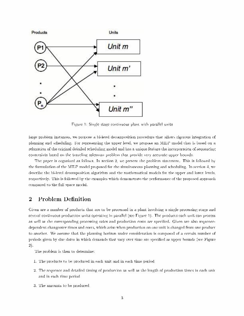
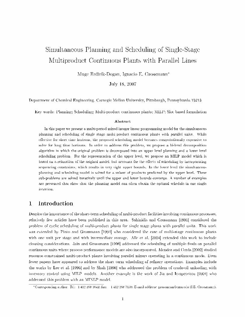
Figure 1: Single stage continuous plant with parallel units

large problem instances, we propose a bi-level decomposition procedure that allows rigorous integration of

planning and scheduling. For representing the upper level, we propose an MILP model that is based on a

relaxation of the original detailed scheduling model and has a unique feature the incorporation of sequencing

constraints based on the traveling salesman problem that provide very accurate upper bounds.

The paper is organized as follows. In section 2, we present the problem statement. This is followed by

the formulation of the MILP model proposed for the simultaneous planning and scheduling. In section 4, we

describe the bi-level decomposition algorithm and the mathematical models for the upper and lower levels,

respectively. This is followed by the examples which demonstrate the performance of the proposed approach

compared to the full space model.

2 Problem De�nition

Given are a number of products that are to be processed in a plant involving a single processing stage and

several continuous production units operating in parallel (see Figure 1). The products each unit can process

as well as the corresponding processing rates and production costs are speci�ed. Given are also sequence-

dependent changeover times and costs, which arise when production on one unit is changed from one product

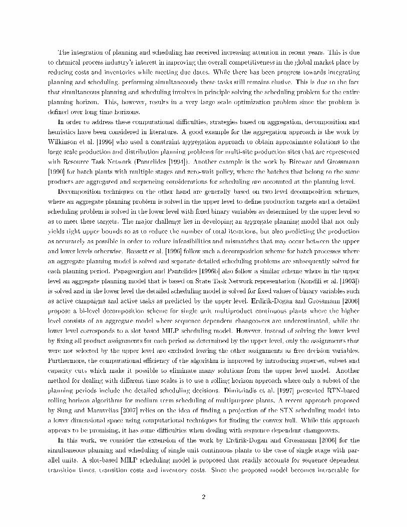
to another. We assume that the planning horizon under consideration is composed of a certain number of

periods given by due dates in which demands that vary over time are speci�ed as upper bounds (see Figure

2).

The problem is then to determine:

1. The products to be produced in each unit and in each time period

2. The sequence and detailed timing of production as well as the length of production times in each unit

and in each time period

3. The amounts to be produced

3

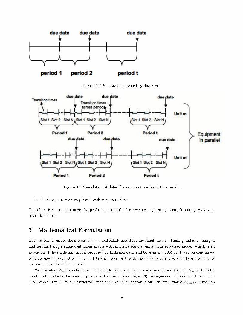
Figure 2: Time periods de�ned by due dates

Figure 3: Time slots postulated for each unit and each time period

4. The change in inventory levels with respect to time

The objective is to maximize the pro�t in terms of sales revenues, operating costs, inventory costs and

transition costs.

3 Mathematical Formulation

This section describes the proposed slot-based MILP model for the simultaneous planning and scheduling of

multiproduct single stage continuous plants with multiple parallel units. The proposed model, which is an

extension of the single unit model proposed by Erdirik-Dogan and Grossmann [2006], is based on continuous

time domain representation. The model parameters, such as demands, due dates, prices, and cost coe�cients

are assumed to be deterministic.

We postulate Nm asynchronous time slots for each unit m for each time period t where Nm is the total

number of products that can be processed by unit m (see Figure 3). Assignments of products to the slots

is to be determined by the model to de�ne the sequence of production. Binary variable Wi,m,l,t is used to

4

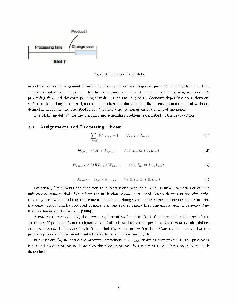
Figure 4: Length of time slots

model the potential assignment of product i to slot l of unit m during time period t. The length of each time

slot is a variable to be determined by the model, and is equal to the summation of the assigned product's

processing time and the corresponding transition time (see Figure 4). Sequence dependent transitions are

activated depending on the assignments of products to slots. The indices, sets, parameters, and variables

de�ned in the model are described in the Nomenclature section given at the end of the paper.

The MILP model (P ) for the planning and scheduling problem is described in the next section.

3.1 Assignments and Processing Times:∑i∈I(m)

Wi,m,l,t = 1 ∀m, l ∈ Lm, t (1)

Θi,m,l,t ≤ Ht ∗Wi,m,l,t ∀ i ∈ Im,m, l ∈, Lm, t (2)

Θi,m,l,t ≥MRTi,m ∗Wi,m,l,t ∀ i ∈ Im,m, l ∈, Lm, t (3)

Xi,m,l,t = ri,m ∗Θi,m,l,t ∀ i ∈, Im,m, l ∈, Lm, t (4)

Equation (1) represents the condition that exactly one product must be assigned to each slot of each

unit at each time period. We enforce the utilization of each postulated slot to circumvent the di�culties

that may arise when modeling the sequence-dependent changeovers across adjacent time periods. Note that

the same product can be produced in more than one slot and more than one unit at each time period (see

Erdirik-Dogan and Grossmann [2006]).

According to constraint (2) the processing time of product i in slot l of unit m during time period t is

set to zero if product i is not assigned to slot l of unit m during time period t. Constraint (2) also de�nes

an upper bound, the length of each time period Ht, on the processing time. Constraint 3 ensures that the

processing time of an assigned product exceeds its minimum run length.

In constraint (4) we de�ne the amount of production Xi,m,l,t, which is proportional to the processing

times and production rates. Note that the production rate is a constant that is both product and unit

dependent.

5

3.2 Transitions:

Transitions arise when production on one unit is changed from one product to another. These transitions

may be associated to a change in the operating conditions or to the cleaning of units.

3.2.1 Transitions within each time period:

In order to take into account sequence-dependent transitions within each time period, we introduce the

transition variable Zi,k,m,l,t.

Zi,k,m,l,t

1 if product i assigned to slot l of unitm is followed by

product k assigned to slot l + 1 of unitmduring time t,

0 otherwise

Wi,m,l,t ∧Wk,m,l+1,t ⇔ Zi,k,m,l,t ∀i, kεI(m), i 6= k, ∀lεLm − {l̄m}, ∀m, ∀t (5)

The proposition in (5) links these transitions variables (Zi,k,m,l,t) with the assignment variables (Wi,m,l,t).

That is, Zi,k,m,l,t should become 1 if and only if product i is assigned to slot l of unit m and product k is

assigned to the consecutive slot (l + 1) of unit m during the same time period. The above logical condition

can be represented by the following inequalities:

Zi,k,m,l,t ≥Wi,m,l,t +Wk,m,l+1,t − 1 ∀i, kεI(m), i 6= k, ∀lεLm − {lm}, ∀m, ∀t (6)

Wi,m,l,t ≥ Zi,k,m,l,t ∀i, k εI(m), i 6= k, ∀m, ∀l ∈, Lm ∀t (7)

Wk,m,l+1,t ≥ Zi,k,m,l,t ∀i, k εI(m), i 6= k, ∀m, ∀εLm − {l̄m}, ∀t (8)

where l̄m is the last slot of unit m for each time period.

Inequalities (7) and (8) can be easily shown to be redundant since the transition variable Zi,k,m,l,t is a

cost item in the objective function and will tend to be zero. Furthermore, using a similar reasoning, the

transition variables Zi,k,m,l,t need not be declared as binaries but may be relaxed in the interval [0,1].

Another way of enforcing the same condition in (5) is to use the following set of propositions :

Wi,m,l,t ⇔∨k∈Im

Zi,k,m,l,t ∀iεI(m),m, l ∈, Lm, t (9)

Wk,m,l+1,t ⇔∨i∈Im

Zi,k,m,l,t ∀kεI(m), m, lεLm − {lm}, t (10)

According to proposition (9), there is exactly one transition from product i in unit m at time period t if and

only if product i is assigned to unit m during time period t. Similarly, according to proposition (10), there

is exactly one transition to product k in unit m during time period t if and only if product k is assigned to

unit m of time period t.

Mathematically, these propositions can be written as follows (see also Sahinidis and Grossmann [1991])

6

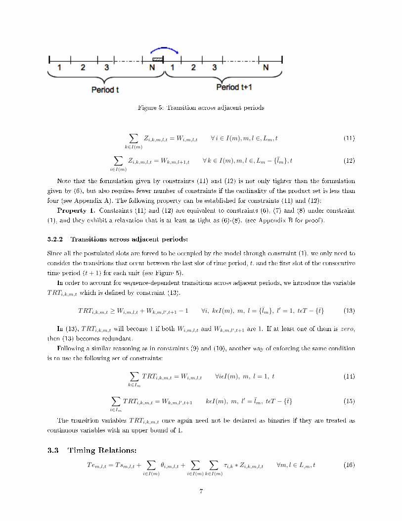
Figure 5: Transition across adjacent periods

∑k∈I(m)

Zi,k,m,l,t = Wi,m,l,t ∀ i ∈ I(m),m, l ∈, Lm, t (11)

∑i∈I(m)

Zi,k,m,l,t = Wk,m,l+1,t ∀ k ∈ I(m),m, l ∈, Lm − {l̄m}, t (12)

Note that the formulation given by constraints (11) and (12) is not only tighter than the formulation

given by (6), but also requires fewer number of constraints if the cardinality of the product set is less than

four (see Appendix A). The following property can be established for constraints (11) and (12):

Property 1. Constraints (11) and (12) are equivalent to constraints (6), (7) and (8) under constraint

(1), and they exhibit a relaxation that is at least as tight as (6)-(8). (see Appendix B for proof).

3.2.2 Transitions across adjacent periods:

Since all the postulated slots are forced to be occupied by the model through constraint (1), we only need to

consider the transitions that occur between the last slot of time period, t, and the �rst slot of the consecutive

time period (t+ 1) for each unit (see Figure 5).

In order to account for sequence-dependent transitions across adjacent periods, we introduce the variable

TRTi,k,m,t which is de�ned by constraint (13).

TRTi,k,m,t ≥Wi,m,l,t +Wk,m,l′,t+1 − 1 ∀i, kεI(m), m, l = {l̄m}, l′ = 1, tεT − {t̄} (13)

In (13), TRTi,k,m,t will become 1 if both Wi,m,l,t and Wk,m,l′,t+1 are 1. If at least one of them is zero,

then (13) becomes redundant.

Following a similar reasoning as in constraints (9) and (10), another way of enforcing the same condition

is to use the following set of constraints:∑k∈Im

TRTi,k,m,t = Wi,m,l,t ∀iεI(m), m, l = 1, t (14)

∑i∈Im

TRTi,k,m,t = Wk,m,l′,t+1 kεI(m), m, l′ = l̄m, tεT − {t̄} (15)

The transition variables TRTi,k,m,t once again need not be declared as binaries if they are treated as

continuous variables with an upper bound of 1.

3.3 Timing Relations:

Tem,l,t = Tsm,l,t +∑

i∈I(m)

θi,m,l,t +∑

i∈I(m)

∑k∈I(m)

τi,k ∗ Zi,k,m,l,t ∀m, l ∈ L,m, t (16)

7

Tsm,l,t+1 ≥ Tem,l′,t +∑

i∈I(m)

∑k∈I(m)

τi,k ∗ TRTi,k,m,t ∀m, l = l̄m, l′ = 1, t ∈ T − {t̄} (17)

Tem,l,t = Tsm,l+1,t ∀m, l ∈ Lm − {l̄m}, t (18)

Tem,l,t ≤ HTt ∀l = l̄m, t (19)

In (16), the end time slot l of unit m during time t is equal to the start time of slot l plus the processing

time of the product assigned to slot l plus the corresponding transition times. Note that according to (1)

and (2), exactly one processing time in the∑iεI(m) θi,m,l,t term is nonzero.

Constraint (17) accounts for the transitions across adjacent time periods. The start time of the �rst slot

of unit m of time period t must be greater than the end time of the last slot of the previous time period

(t − 1) summed with the corresponding transition time between the time periods. According to (18), the

end time of each slot must be equal to the start time of the consecutive slot. Constraint (19) ensures that

the end time of the last slot of period t is less than or equal to the end time of time period t.

3.4 Inventory Balances and Costs:

INVi,t = INV Ii +∑m∈Mi

ri,m ∗∑l∈Lm

θi,m,l,t ∀i, t = 1 (20)

INVi,t = INV Oi,t−1 +∑m∈Mi

ri,m ∗∑l∈Lm

θi,m,l,t ∀i, t 6= 1 (21)

INV Oi,t = INVi,t − Si,t ∀i, t (22)

Areai,t ≥ INV Oi,,t−1 ∗Ht + (∑mεMi

ri,m ∗∑l∈Lm

θi,m,l,t) ∗Ht ∀i, t (23)

Equation (20) de�nes the inventory level of product i at the end of the �rst time period as the summation

of the initial inventory for product i and the amount of product i produced in the �rst time period. In

equation (21), the inventory level of product i at the end of time t is equal to the sum of the �nal inventory

level of product i at the end of time period t− 1, and the amount of product i produced during time period

t. In constraint (22) the �nal inventory level of product i at the end of time period t is de�ned as the

inventory level after the demands are satis�ed at the end of each time period. As for the inventory cost, we

use constraint(23), which is a linear overestimation as discussed in Erdirik-Dogan and Grossmann (2006).

3.5 Demand:

Si,t ≥ di,t ∀i, t (24)

Constraint (24) states that the demands must be satis�ed or exceeded for all products in the plant at the

due dates, which correspond to the end time of each period. Note that demands to be satis�ed are de�ned

as lower bounds. If the demands are too high this might lead to infeasible solutions. To guard against such

a case, one can add a slack variable,∆i,t, to constraint (24) to yield constraint (25) and subtract the term

8

∑i

∑t Peni,t ∗ ∆i,tfrom the objective function (26) wherePeni,t is a penalty cost. In this way the model

would yield a solution that minimizes violations of demand constraints. The application of these constraints

and derivation of a schedule with tardy delivery of orders are given in Example 5.

Si,t + ∆i,t ≥ di,t ∀i, t (25)

3.6 Objective Function:

ZP =∑i

∑t

CPi,t ∗ Si,t −∑i

∑t

CINVi,t ∗Areai,t −∑t

∑m

∑iεI(m)

COPi,t ∗ X̃i,t −

∑i

∑k

∑m

∑t

∑l

[TRANSi,k ∗ Zi,k,m,l,t − CTRANSi,k ∗ TRTi,k,m,t

](26)

The objective is to maximize the pro�t (26), which is given by the sum of sales revenues, the inventory costs,

operating costs, the transition costs within each week and transition costs across adjacent weeks.

We should note that for the case when the same product is assigned to more than one slot of the same

unit in the same time period, the consecutive utilization of the slots is ensured by optimality. Since the

inventory costs have been overestimated, assigning the same product to non-consecutive slots will yield the

same inventory cost as assigning the same product to consecutive slots. Furthermore, since assignment of

the same product to non-consecutive slots will result in an increase in the transition costs, we do not need

to enforce the consecutive utilization of slots by the same product. As an example, see Figure 6, where both

solutions result in the same total inventory costs shown by the shaded area. However, the solution shown in

Figure 6a results in higher transition costs as it has two more transitions than the solution shown in Figure

6b.

We should also note that allowing the assignment of the same product to more than one slot of the

same unit in the same time period, combined with the fact that slots have variable lengths, increases the

degeneracy of the problem (Figure 7). This is due to the fact that allocation of the total processing times of

the assigned products to slots in any feasible way within a time period, while preserving the original sequence,

will result in several alternative optima. In order to avoid this degeneracy, we introduce symmetry breaking

constraints as proposed by Erdirik-Dogan and Grossmann [2006]. Note that degeneracy in a time period

occurs if the total number of available slots (Nm) is greater than the total number of products assigned to

that time period (∑i Y OPi,t). In other words degeneracy occurs if the number of �exible slots is greater

than zero (FS = N −∑i Y OPi,t). The idea of the symmetry breaking constraints is to enforce the product

that is assigned to the �rst slot to be allocated to FS number of additional slots, hence leaving just one

available slot for the rest of the assigned products. For the example shown in Figure 7, introducing symmetry

breaking constraints reduces the feasible solutions only to the solution presented in Figure 7a.

As shown by Erdirik-Dogan and Grossmann [2006], the symmetry-breaking constraints can be written

as,

Y OPi,m,t ≥Wi,m,l,t ∀iεI(m), ∀m, ∀l ∈ Lm, ∀t (27)

Y OPi,m,t ≤ NYi,m,t ≤ Nm ∗ Y OPi,m,t ∀iεI(m), ∀m, ∀t (28)

9

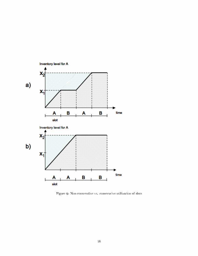
Figure 6: Non-consecutive vs. consecutive utilization of slots

10

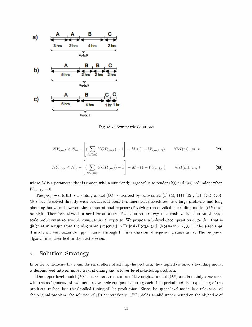
Figure 7: Symmetric Solutions

NYi,m,t ≥ Nm −

(∑iεI(m)

Y OPi,m,t)− 1

−M ∗ (1−Wi,m,1,t)) ∀iεI(m), m, t (29)

NYi,m,t ≤ Nm −

(∑

kεI(m)

Y OPk,m,t)− 1

−M ∗ (1−Wi,m,1,t)) ∀iεI(m), m, t (30)

whereM is a parameter that is chosen with a su�ciently large value to render (29) and (30) redundant when

Wi,m,1,t = 0.The proposed MILP scheduling model (OP ) described by constraints (1)-(4), (11)-(12), (14)-(24), (26)-

(30) can be solved directly with branch and bound enumeration procedures. For large problems and long

planning horizons, however, the computational expense of solving the detailed scheduling model (OP ) can

be high. Therefore, there is a need for an alternative solution strategy that enables the solution of large-

scale problems at reasonable computational expense. We propose a bi-level decomposition algorithm that is

di�erent in nature from the algorithm presented in Erdirik-Dogan and Grossmann [2006] in the sense that

it involves a very accurate upper bound through the introduction of sequencing constraints. The proposed

algorithm is described in the next section.

4 Solution Strategy

In order to decrease the computational e�ort of solving the problem, the original detailed scheduling model

is decomposed into an upper level planning and a lower level scheduling problem.

The upper level model (P ) is based on a relaxation of the original model (OP ) and is mainly concerned

with the assignments of products to available equipment during each time period and the sequencing of the

products, rather than the detailed timing of the production. Since the upper level model is a relaxation of

the original problem, the solution of (P ) at iteration r, (P r), yields a valid upper bound on the objective of

11

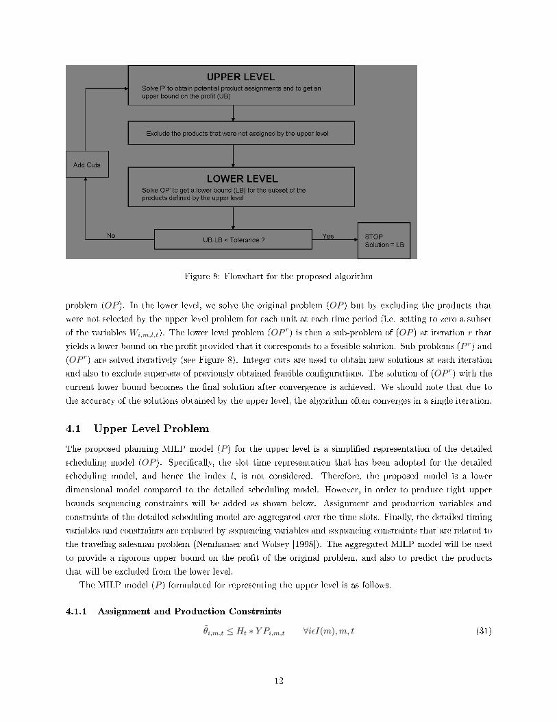
Figure 8: Flowchart for the proposed algorithm

problem (OP ). In the lower level, we solve the original problem (OP ) but by excluding the products that

were not selected by the upper level problem for each unit at each time period (i.e. setting to zero a subset

of the variables Wi,m,l,t). The lower level problem (OP r) is then a sub-problem of (OP ) at iteration r that

yields a lower bound on the pro�t provided that it corresponds to a feasible solution. Sub-problems (P r) and

(OP r) are solved iteratively (see Figure 8). Integer cuts are used to obtain new solutions at each iteration

and also to exclude supersets of previously obtained feasible con�gurations. The solution of (OP r) with the

current lower bound becomes the �nal solution after convergence is achieved. We should note that due to

the accuracy of the solutions obtained by the upper level, the algorithm often converges in a single iteration.

4.1 Upper Level Problem

The proposed planning MILP model (P ) for the upper level is a simpli�ed representation of the detailed

scheduling model (OP ). Speci�cally, the slot time representation that has been adopted for the detailed

scheduling model, and hence the index l, is not considered. Therefore, the proposed model is a lower

dimensional model compared to the detailed scheduling model. However, in order to produce tight upper

bounds sequencing constraints will be added as shown below. Assignment and production variables and

constraints of the detailed scheduling model are aggregated over the time slots. Finally, the detailed timing

variables and constraints are replaced by sequencing variables and sequencing constraints that are related to

the traveling salesman problem (Nemhauser and Wolsey [1998]). The aggregated MILP model will be used

to provide a rigorous upper bound on the pro�t of the original problem, and also to predict the products

that will be excluded from the lower level.

The MILP model (P ) formulated for representing the upper level is as follows.

4.1.1 Assignment and Production Constraints

θ̃i,m,t ≤ Ht ∗ Y Pi,m,t ∀iεI(m),m, t (31)

12

X̃i,m,t = ri,m ∗ θ̃i,m,t ∀iεI(m),m, t (32)

Since the sequencing of the products is no longer de�ned through slots, we introduce the binary variable,

Y Pi,m,t, which represents the assignment of product i to unit m during time period t. We also introduce

aggregate variables, θ̃i,m,t =∑l θi,m,l,t, and X̃i,m,t =

∑lXi,m,l,t. Constraint (31) is obtained by summing

constraint (2) over l and replacing θi,m,l,t by θ̃i,m,t and∑lWi,m,l,t by Y Pi,m,t (see Erdirik-Dogan and

Grossmann [2006]). Constraint (32) is obtained by summing constraint (4) over l and replacing Xi,m,l,t by

X̃i,m,t and θi,m,l,t by θ̃i,m,t.

4.1.2 Inventory Balances and Costs

INVi,t = INV Ii,t−1 +∑mεMi

ri,m ∗ θ̃i,m,t ∀i, t (33)

INVi,t = INV Oi,t−1 +∑mεMi

ri,m ∗ θ̃i,m,t ∀i, t (34)

INV Oi,t = INVi,t − Si,t ∀i, t (35)

Areai,t ≥ (INV Oi,t−1) ∗Ht + (∑mεMi

ri,m ∗ θ̃i,m,t) ∗Ht ∀i, t (36)

Constraints (33), (34), (35) and (36) are in essence the same as (20), (21), (22) and (23) except that∑l θi,m,l,tis replaced by the aggregate variable θ̃i,m,t.

4.1.3 Demand

Si,t ≥ Di,t ∀i, t (37)

Constraint (37) is the same as (24).

4.1.4 Sequencing Constraints

As stated before, the proposed upper level model is based on ignoring the detailed timing constraints and is

only concerned with determining the sequence of production on each unit during each time period. Hence, we

ignore the detailed timing constraints (6 - 19) and determine the optimal sequence via sequencing constraints

which have been proposed by Erdirik-Dogan and Grossmann [submitted 2007] for the case of parallel batch

reactors. The extension of these constraints to the case of continuous plants is direct. We include a brief

explanation of these constraints, although the equations are similar as in Erdirik-Dogan and Grossmann

[submitted 2007].

The basic idea is �rst to generate a cyclic schedule for each unit within each time period, where the

transition times amongst the assigned products are minimized. Then, to determine the optimal sequence

for each unit in each time period one of the links in the cycle is broken (see example in Figure 9). Since

the transition times are assumed to be directly proportional to the transition costs, the link to be broken

will correspond to the pair with the highest transition time, thus resulting in the minimum transition time

sequence in each time period.

13

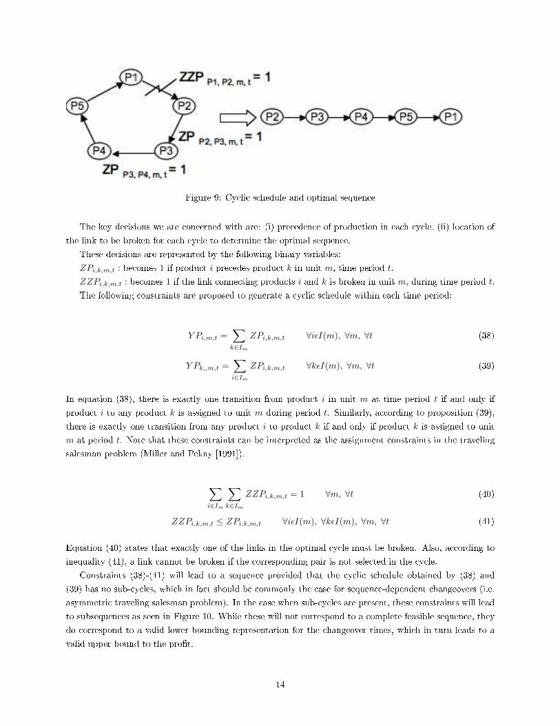
Figure 9: Cyclic schedule and optimal sequence

The key decisions we are concerned with are: (i) precedence of production in each cycle, (ii) location of

the link to be broken for each cycle to determine the optimal sequence.

These decisions are represented by the following binary variables:

ZPi,k,m,t : becomes 1 if product i precedes product k in unit m, time period t.

ZZPi,k,m,t : becomes 1 if the link connecting products i and k is broken in unit m, during time period t.

The following constraints are proposed to generate a cyclic schedule within each time period:

Y Pi,m,t =∑k∈Im

ZPi,k,m,t ∀iεI(m), ∀m, ∀t (38)

Y Pk,,m,t =∑i∈Im

ZPi,k,m,t ∀kεI(m), ∀m, ∀t (39)

In equation (38), there is exactly one transition from product i in unit m at time period t if and only if

product i to any product k is assigned to unit m during period t. Similarly, according to proposition (39),

there is exactly one transition from any product i to product k if and only if product k is assigned to unit

m at period t. Note that these constraints can be interpreted as the assignment constraints in the traveling

salesman problem (Miller and Pekny [1991]).

∑i∈Im

∑k∈Im

ZZPi,k,m,t = 1 ∀m, ∀t (40)

ZZPi,k,m,t ≤ ZPi,k,m,t ∀iεI(m), ∀kεI(m), ∀m, ∀t (41)

Equation (40) states that exactly one of the links in the optimal cycle must be broken. Also, according to

inequality (41), a link cannot be broken if the corresponding pair is not selected in the cycle.

Constraints (38)-(41) will lead to a sequence provided that the cyclic schedule obtained by (38) and

(39) has no sub-cycles, which in fact should be commonly the case for sequence-dependent changeovers (i.e.

asymmetric traveling salesman problem). In the case when sub-cycles are present, these constraints will lead

to subsequences as seen in Figure 10. While these will not correspond to a complete feasible sequence, they

do correspond to a valid lower bounding representation for the changeover times, which in turn leads to a

valid upper bound to the pro�t.

14

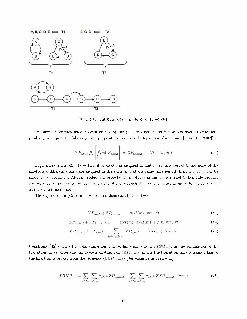
Figure 10: Subsequences in presence of sub-cycles

We should note that since in constraints (38) and (39), products i and k may correspond to the same

product, we impose the following logic proposition (see Erdirik-Dogan and Grossmann [submitted 2007]):

Y Pi,m,t∧∧

k 6=i

¬Y Pk,m,t

⇔ ZPi,i,m,t ∀i ∈ Im,m, t (42)

Logic proposition (42) states that if product i is assigned in unit m at time period t, and none of the

products k di�erent than i are assigned in the same unit at the same time period, then product i can be

preceded by product i. Also, if product i is preceded by product i in unit m at period t, then only product

i is assigned in unit m for period t, and none of the products k other than i are assigned to the same unit

at the same time period.

The expression in (42) can be written mathematically as follows:

Y Pim,t ≥ ZPi,i,m,t ∀iεI(m), ∀m, ∀t (43)

ZPi,i,m,t + Y Pk,m,t ≤ 1 ∀iεI(m), ∀kεI(m), i 6= k, ∀m, ∀t (44)

ZPi,i,m,t ≥ Y Pi,m,t −∑

k 6=i,kεI(m)

Y Pk,m,t ∀iεI(m), ∀m, ∀t (45)

Constraint (46) de�nes the total transition time within each period, TRNPm,t, as the summation of the

transition times corresponding to each existing pair (ZPi,k,m,t) minus the transition time corresponding to

the link that is broken from the sequence (ZZPi,k,m,t) (See example in Figure 11).

TRNPm,t =∑i∈Im

∑k∈Im

τi,k ∗ ZPi,k,m,t −∑i∈Im

∑k∈Im

τi,k ∗ ZZPi,k,m,t ∀m, t (46)

15

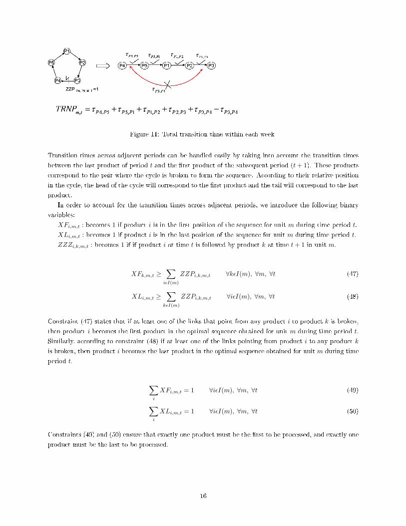
Figure 11: Total transition time within each week

Transition times across adjacent periods can be handled easily by taking into account the transition times

between the last product of period t and the �rst product of the subsequent period (t+ 1). These productscorrespond to the pair where the cycle is broken to form the sequence. According to their relative position

in the cycle, the head of the cycle will correspond to the �rst product and the tail will correspond to the last

product.

In order to account for the transition times across adjacent periods, we introduce the following binary

variables:

XFi,m,t : becomes 1 if product i is in the �rst position of the sequence for unit m during time period t.

XLi,m,t : becomes 1 if product i is in the last position of the sequence for unit m during time period t.

ZZZi,k,m,t : becomes 1 if if product i at time t is followed by product k at time t+ 1 in unit m.

XFk,m,t ≥∑iεI(m)

ZZPi,k,m,t ∀kεI(m), ∀m, ∀t (47)

XLi,m,t ≥∑

kεI(m)

ZZPi,k,m,t ∀iεI(m), ∀m, ∀t (48)

Constraint (47) states that if at least one of the links that point from any product i to product k is broken,

then product i becomes the �rst product in the optimal sequence obtained for unit m during time period t.

Similarly, according to constraint (48) if at least one of the links pointing from product i to any product k

is broken, then product i becomes the last product in the optimal sequence obtained for unit m during time

period t.

∑i

XFi,m,t = 1 ∀iεI(m), ∀m, ∀t (49)

∑i

XLi,m,t = 1 ∀iεI(m), ∀m, ∀t (50)

Constraints (49) and (50) ensure that exactly one product must be the �rst to be processed, and exactly one

product must be the last to be processed.

16

∑kεI(m)

ZZZi,k,m,t = XLi,m,t ∀iεI(m), ∀m, ∀t (51)

∑iεI(m)

ZZZi,k,m,t = XFk,m,t+1 ∀kεI(m), ∀m, ∀tεT − {t̄} (52)

Constraints (51) and (52) de�ne the transition variable that accounts for transitions across adjacent weeks,

ZZZi,k,m,t. In (51) , exactly one transition occurs from product i at the end of time period t in unit m, if

and only if i is the last produced last at time period t. Similarly, according to (52), exactly one transition

to product i′ occurs at the beginning of time period t+ 1 in unit m if and only if product i′ is produced the

�rst at time period t+ 1 in unit m.

4.1.5 Time Balance

∑iεI(m)

θ̃i,m,t + TRNPm,t +

∑iεI(m)

∑kεI(m)

τi,k ∗ ZZZi,k,m,t

≤ Ht ∀t (53)

In constraint (53), summation of the processing times of the products assigned to unit m during time period

t, plus the total transition time within that time period, plus the transition time to the adjacent time period,

cannot exceed the length of that time period.

4.1.6 Objective function

Profit =∑i

∑t

CPi,t ∗ Si,t −∑i

∑t

CINVi,t ∗Areai,t −∑t

∑i

COPi,t ∗ X̃i,t

−∑t

∑m

∑iεI(m)

∑kεI(m)

CTRANSi,k ∗ (ZPi,k,m,t)

−∑t

∑m

∑iεI(m)

∑kεI(m)

CTRANSi,k ∗ (ZZZi,k,m,t − ZZPi,k,mt) (54)

The objective is to maximize pro�t in terms of sales minus inventory costs, operating costs and transition

costs. The last three terms of the objective function stand for the transition costs: third to last accounts

for the transition costs within each cycle, the second to last stands for the transition cost of the link that

was broken, and the last term stands for the transition costs of the changeovers that occur across adjacent

weeks.

The upper level planning problem (P ) is then given by constraints (31)-(54).

4.2 Lower-Level Problem

In the lower level, the original detailed scheduling model (OP ) is solved for a subset of products as determined

by the upper level. Speci�cally, products that are predicted to be produced by the upper level, may or may

not be produced by the lower level. However, those products which were predicted as not to be produced

by the upper level, are excluded from the lower level in each unit during each time period by setting the

17

corresponding binary variables to zero. Solving the original detailed model (OP ) in a reduced space makes

it possible to greatly expedite the solution of the corresponding MILP model.

Y OPi,m,t ≤ Y P ri,m,t ∀i ∈ Im,m, t (55)

The above condition is enforced by the inequality in (55). The lower level problem (OP r) is then described

by constraints (1)-(4), (11)-(12), (14)-(30) and (55).

4.3 Integer Cuts

After each iteration, if the bounds obtained from the upper level model and the lower level model do not lie

within a speci�ed tolerance, we must obtain a new solution from the upper level model. We incorporate into

the upper level model integer cuts to generate new solutions in terms of the assignment variable Y Pi,m,t.

The simplest and weakest cut that excludes the previously obtained feasible solutions from the upper level

model is as follows (Balas and Jeroslow [1972]),

∑(i,t)εZr

1

Y Pi,m,t −∑

(i,t)εZr0

Y Pi,m,t ≤ |Zr1 | − 1 (56)

where Zr0 ={i, t∣∣Y P ri,m,t = 0

}and Zr1 =

{i, t∣∣Y P ri,m,t = 1

}Note that Zr0 and Zr1 are obtained from the optimal solution at the upper level in terms of the assignment

variable in iteration r.

Instead of using the integer cut in (56), we can use the cover cut which is stronger in the sense that it does

not only exclude the current assignment r but also any other assignment that is a superset of assignment r.

The general form of the cover cuts is as follows,

∑(i,t)εZr

1

Y Pi,m,t ≤ |Zr1 | − 1 (57)

The justi�cation of excluding supersets is due to the fact that any superset implies adding an additional

product which as a consequence results in an increase in transition times and costs thereby decrease in the

pro�t. We should also note that the extension of superset and subset cuts presented in Erdirik-Dogan and

Grossmann [2006] to the parallel units case is direct. However, we did not include them in this paper since

the algorithm often converges in one single iteration as shown in the results section.

5 Remarks

1. The proposed decomposition scheme is rigorous and guarantees the global optimal solution in a �nite

number of iterations.

2. For the case when there are no sub-cycles, the solution obtained by the upper level planning model

(P ) is identical to the one obtained by the original detailed model (OP ) since the upper level model

(P ) rigorously accounts for the sequence-dependent changeover times and costs. Hence, in this case

the algorithm converges in one single iteration.

3. When the upper level model (P ) exhibits sub-cycles, a valid upper bound on the pro�t is obtained

since constraints (38) -(41) represent a relaxation to the traveling salesman problem.

18

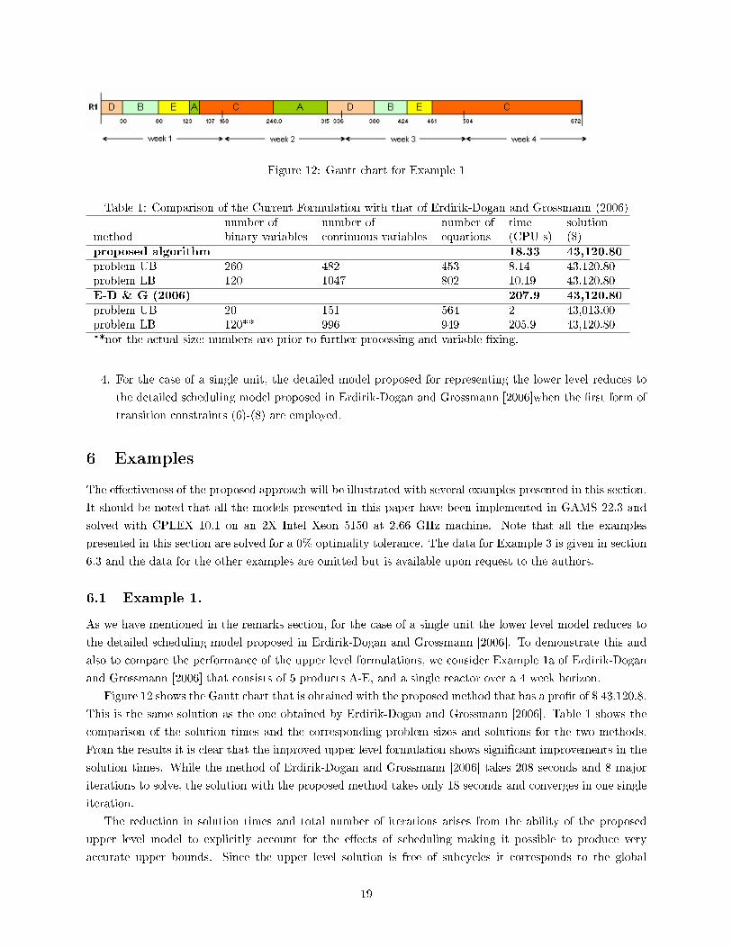
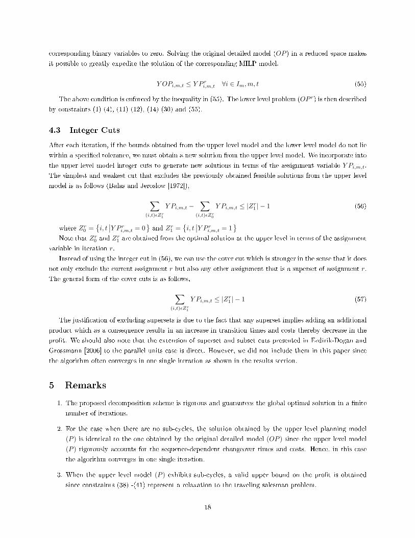
Figure 12: Gantt chart for Example 1

Table 1: Comparison of the Current Formulation with that of Erdirik-Dogan and Grossmann (2006)number of number of number of time solution

method binary variables continuous variables equations (CPU s) ($)proposed algorithm 18.33 43,120.80problem UB 260 482 453 8.14 43,120.80problem LB 120 1047 802 10.19 43,120.80E-D & G (2006) 207.9 43,120.80problem UB 20 151 564 2 43,013.00problem LB 120** 996 949 205.9 43,120.80**not the actual size; numbers are prior to further processing and variable �xing.

4. For the case of a single unit, the detailed model proposed for representing the lower level reduces to

the detailed scheduling model proposed in Erdirik-Dogan and Grossmann [2006]when the �rst form of

transition constraints (6)-(8) are employed.

6 Examples

The e�ectiveness of the proposed approach will be illustrated with several examples presented in this section.

It should be noted that all the models presented in this paper have been implemented in GAMS 22.3 and

solved with CPLEX 10.1 on an 2X Intel Xeon 5150 at 2.66 GHz machine. Note that all the examples

presented in this section are solved for a 0% optimality tolerance. The data for Example 3 is given in section

6.3 and the data for the other examples are omitted but is available upon request to the authors.

6.1 Example 1.

As we have mentioned in the remarks section, for the case of a single unit the lower level model reduces to

the detailed scheduling model proposed in Erdirik-Dogan and Grossmann [2006]. To demonstrate this and

also to compare the performance of the upper level formulations, we consider Example 1a of Erdirik-Dogan

and Grossmann [2006] that consists of 5 products A-E, and a single reactor over a 4 week horizon.

Figure 12 shows the Gantt chart that is obtained with the proposed method that has a pro�t of $ 43,120.8.

This is the same solution as the one obtained by Erdirik-Dogan and Grossmann [2006]. Table 1 shows the

comparison of the solution times and the corresponding problem sizes and solutions for the two methods.

From the results it is clear that the improved upper level formulation shows signi�cant improvements in the

solution times. While the method of Erdirik-Dogan and Grossmann [2006] takes 208 seconds and 8 major

iterations to solve, the solution with the proposed method takes only 18 seconds and converges in one single

iteration.

The reduction in solution times and total number of iterations arises from the ability of the proposed

upper level model to explicitly account for the e�ects of scheduling making it possible to produce very

accurate upper bounds. Since the upper level solution is free of subcycles it corresponds to the global

19

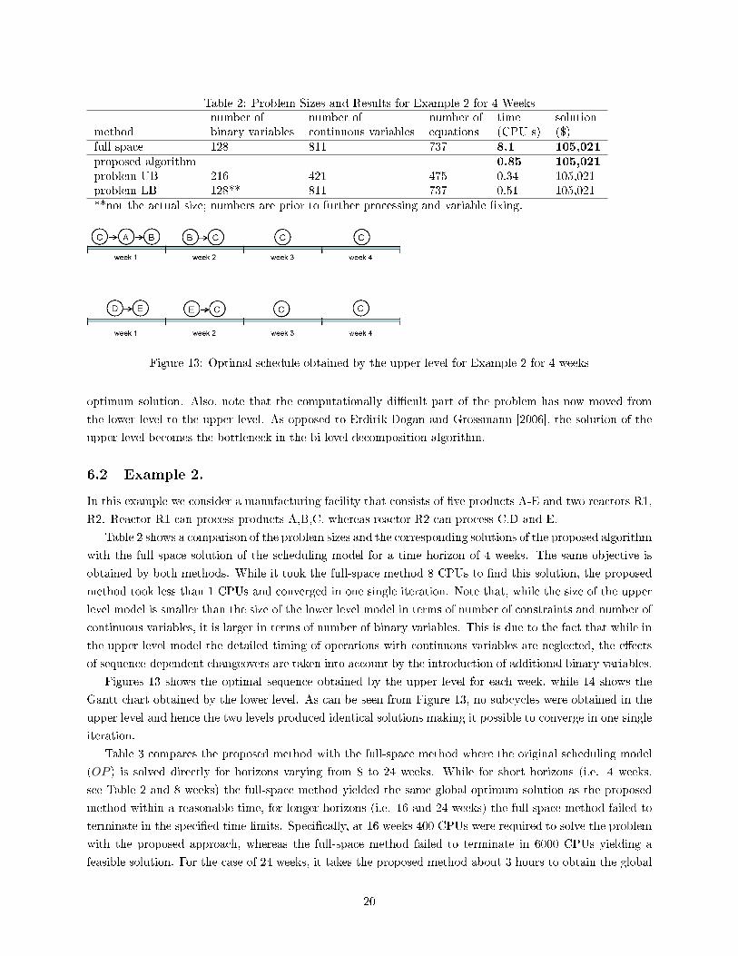
Table 2: Problem Sizes and Results for Example 2 for 4 Weeksnumber of number of number of time solution

method binary variables continuous variables equations (CPU s) ($)full space 128 811 737 8.1 105,021proposed algorithm 0.85 105,021problem UB 216 421 475 0.34 105,021problem LB 128** 811 737 0.51 105,021**not the actual size; numbers are prior to further processing and variable �xing.

Figure 13: Optimal schedule obtained by the upper level for Example 2 for 4 weeks

optimum solution. Also, note that the computationally di�cult part of the problem has now moved from

the lower level to the upper level. As opposed to Erdirik-Dogan and Grossmann [2006], the solution of the

upper level becomes the bottleneck in the bi-level decomposition algorithm.

6.2 Example 2.

In this example we consider a manufacturing facility that consists of �ve products A-E and two reactors R1,

R2. Reactor R1 can process products A,B,C, whereas reactor R2 can process C,D and E.

Table 2 shows a comparison of the problem sizes and the corresponding solutions of the proposed algorithm

with the full space solution of the scheduling model for a time horizon of 4 weeks. The same objective is

obtained by both methods. While it took the full-space method 8 CPUs to �nd this solution, the proposed

method took less than 1 CPUs and converged in one single iteration. Note that, while the size of the upper

level model is smaller than the size of the lower level model in terms of number of constraints and number of

continuous variables, it is larger in terms of number of binary variables. This is due to the fact that while in

the upper level model the detailed timing of operations with continuous variables are neglected, the e�ects

of sequence-dependent changeovers are taken into account by the introduction of additional binary variables.

Figures 13 shows the optimal sequence obtained by the upper level for each week, while 14 shows the

Gantt chart obtained by the lower level. As can be seen from Figure 13, no subcycles were obtained in the

upper level and hence the two levels produced identical solutions making it possible to converge in one single

iteration.

Table 3 compares the proposed method with the full-space method where the original scheduling model

(OP ) is solved directly for horizons varying from 8 to 24 weeks. While for short horizons (i.e. 4 weeks,

see Table 2 and 8 weeks) the full-space method yielded the same global optimum solution as the proposed

method within a reasonable time, for longer horizons (i.e. 16 and 24 weeks) the full-space method failed to

terminate in the speci�ed time limits. Speci�cally, at 16 weeks 400 CPUs were required to solve the problem

with the proposed approach, whereas the full-space method failed to terminate in 6000 CPUs yielding a

feasible solution. For the case of 24 weeks, it takes the proposed method about 3 hours to obtain the global

20

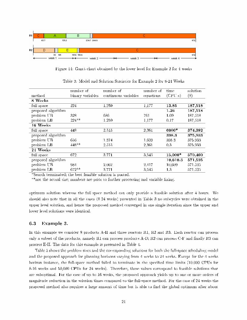
Figure 14: Gantt chart obtained by the lower level for Example 2 for 4 weeks

Table 3: Model and Solution Statistics for Example 2 for 8-24 Weeks

number of number of number of time solutionmethod binary variables continuous variables equations (CPU s) ($)8 Weeksfull space 224 1,259 1,177 13.85 187,518proposed algorithm 1.26 187,518problem UB 328 686 761 1.09 187,518problem LB 224** 1,259 1,177 0.17 187,51816 Weeksfull space 448 2,515 2,361 6000* 374,392proposed algorithm 398.3 375,933problem UB 656 1,374 1,609 398.3 375,933problem LB 448** 2,515 2,361 0.3 375,93324 Weeksfull space 672 3,771 3,545 15,000* 570,400proposed algorithm 10,610.3 571,525problem UB 984 2,062 2,417 10,609 571,525problem LB 672** 3,771 3,545 1.3 571,525*Search terminated; the best feasible solution is posted.**not the actual size; numbers are prior to further processing and variable �xing.

optimum solution whereas the full-space method can only provide a feasible solution after 4 hours. We

should also note that in all the cases (8-24 weeks) presented in Table 3 no subcycles were obtained in the

upper level solution, and hence the proposed method converged in one single iteration since the upper and

lower level solutions were identical.

6.3 Example 3.

In this example we consider 8 products A-H and three reactors R1, R2 and R3. Each reactor can process

only a subset of the products, namely R1 can process products A-D; R2 can process C-F and �nally R3 can

process E-H. The data for this example is presented in Table 4.

Table 5 shows the problem sizes and the corresponding solutions for both the full-space scheduling model

and the proposed approach for planning horizons varying from 4 weeks to 24 weeks. Except for the 4 weeks

horizon instance, the full-space method failed to terminate in the speci�ed time limits (10,000 CPUs for

8-16 weeks and 50,000 CPUs for 24 weeks). Therefore, these values correspond to feasible solutions that

are suboptimal. For the case of up to 16 weeks, the proposed approach yields up to one or more orders of

magnitude reduction in the solution times compared to the full-space method. For the case of 24 weeks the

proposed method also requires a large amount of time but is able to �nd the global optimum after about

21

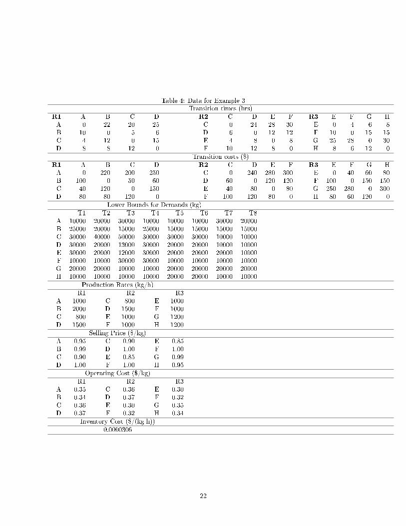
Table 4: Data for Example 3Transition times (hrs)

R1 A B C D R2 C D E F R3 E F G HA 0 22 20 25 C 0 24 28 30 E 0 4 6 8B 10 0 5 6 D 6 0 12 12 F 10 0 15 15C 4 12 0 15 E 4 8 0 8 G 25 28 0 30D 8 8 12 0 F 10 12 8 0 H 8 6 12 0

Transition costs ($)R1 A B C D R2 C D E F R3 E F G HA 0 220 200 250 C 0 240 280 300 E 0 40 60 80B 100 0 50 60 D 60 0 120 120 F 100 0 150 150C 40 120 0 150 E 40 80 0 80 G 250 280 0 300D 80 80 120 0 F 100 120 80 0 H 80 60 120 0

Lower Bounds for Demands (kg)T1 T2 T3 T4 T5 T6 T7 T8

A 10000 20000 30000 10000 10000 10000 30000 20000B 25000 20000 15000 25000 15000 15000 15000 15000C 30000 40000 50000 30000 30000 30000 10000 10000D 30000 20000 13000 30000 20000 20000 10000 10000E 30000 20000 12000 30000 20000 20000 20000 10000F 10000 10000 30000 30000 10000 10000 10000 10000G 20000 20000 10000 10000 20000 20000 20000 20000H 10000 10000 10000 10000 20000 20000 10000 10000

Production Rates (kg/h)R1 R2 R3

A 1000 C 800 E 1000B 2000 D 1500 F 1000C 800 E 1000 G 1200D 1500 F 1000 H 1200

Selling Price ($/kg)A 0.95 C 0.90 E 0.85B 0.99 D 1.00 F 1.00C 0.90 E 0.85 G 0.99D 1.00 F 1.00 H 0.95

Operating Cost ($/kg)R1 R2 R3

A 0.35 C 0.36 E 0.30B 0.34 D 0.37 F 0.32C 0.36 E 0.30 G 0.35D 0.37 F 0.32 H 0.34

Inventory Cost ($/(kg h))0.0000306

22

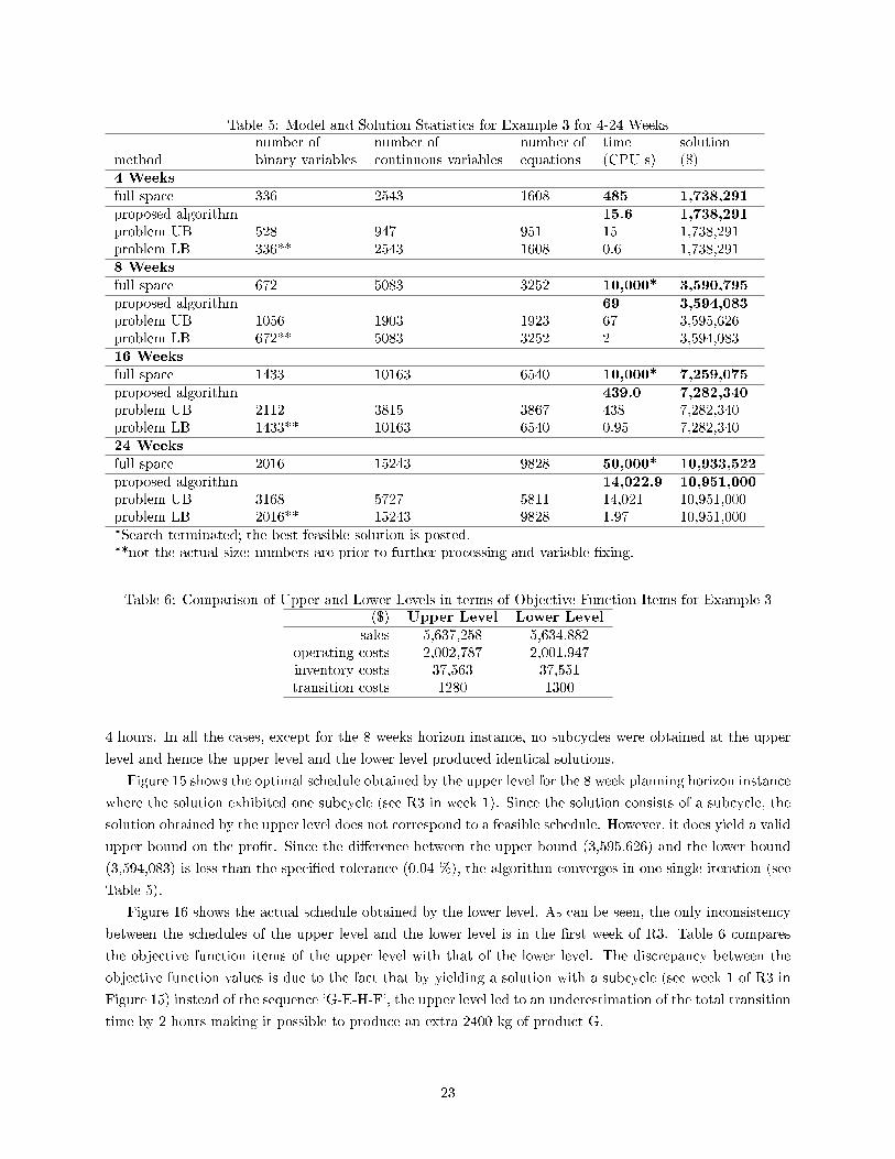
Table 5: Model and Solution Statistics for Example 3 for 4-24 Weeksnumber of number of number of time solution

method binary variables continuous variables equations (CPU s) ($)4 Weeksfull space 336 2543 1608 485 1,738,291proposed algorithm 15.6 1,738,291problem UB 528 947 951 15 1,738,291problem LB 336** 2543 1608 0.6 1,738,2918 Weeksfull space 672 5083 3252 10,000* 3,590,795proposed algorithm 69 3,594,083problem UB 1056 1903 1923 67 3,595,626problem LB 672** 5083 3252 2 3,594,08316 Weeksfull space 1433 10163 6540 10,000* 7,259,075proposed algorithm 439.0 7,282,340problem UB 2112 3815 3867 438 7,282,340problem LB 1433** 10163 6540 0.95 7,282,34024 Weeksfull space 2016 15243 9828 50,000* 10,933,522proposed algorithm 14,022.9 10,951,000problem UB 3168 5727 5811 14,021 10,951,000problem LB 2016** 15243 9828 1.97 10,951,000*Search terminated; the best feasible solution is posted.**not the actual size; numbers are prior to further processing and variable �xing.

Table 6: Comparison of Upper and Lower Levels in terms of Objective Function Items for Example 3($) Upper Level Lower Level

sales 5,637,258 5,634,882operating costs 2,002,787 2,001,947inventory costs 37,563 37,551transition costs 1280 1300

4 hours. In all the cases, except for the 8 weeks horizon instance, no subcycles were obtained at the upper

level and hence the upper level and the lower level produced identical solutions.

Figure 15 shows the optimal schedule obtained by the upper level for the 8 week planning horizon instance

where the solution exhibited one subcycle (see R3 in week 1). Since the solution consists of a subcycle, the

solution obtained by the upper level does not correspond to a feasible schedule. However, it does yield a valid

upper bound on the pro�t. Since the di�erence between the upper bound (3,595,626) and the lower bound

(3,594,083) is less than the speci�ed tolerance (0.04 %), the algorithm converges in one single iteration (see

Table 5).

Figure 16 shows the actual schedule obtained by the lower level. As can be seen, the only inconsistency

between the schedules of the upper level and the lower level is in the �rst week of R3. Table 6 compares

the objective function items of the upper level with that of the lower level. The discrepancy between the

objective function values is due to the fact that by yielding a solution with a subcycle (see week 1 of R3 in

Figure 15) instead of the sequence 'G-E-H-F', the upper level led to an underestimation of the total transition

time by 2 hours making it possible to produce an extra 2400 kg of product G.

23

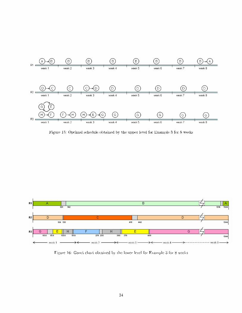
Figure 15: Optimal schedule obtained by the upper level for Example 3 for 8 weeks

Figure 16: Gantt chart obtained by the lower level for Example 3 for 8 weeks

24

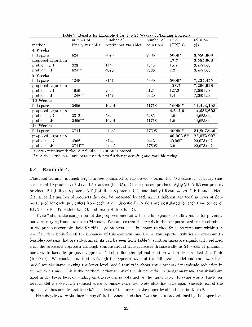
Table 7: Results for Example 4 for 4 to 24 Weeks of Planning Horizonsnumber of number of number of time solution

method binary variables continuous variables equations (CPU s) ($)4 Weeksfull space 624 4075 2886 5000* 3,550,009proposed algorithm 17.7 3,555,060problem UB 828 1444 1545 15.5 3,555,060problem LB 624** 4075 2886 2.2 3,555,0608 Weeksfull space 1248 8147 5830 5000* 7,235,455proposed algorithm 128.7 7,266,038problem UB 1656 2904 3125 127.3 7,266,038problem LB 1248** 8147 5830 1.4 7,266,03816 Weeksfull space 2496 16291 11718 10000* 14,443,198proposed algorithm 4,612.6 14,685,603problem UB 3312 5824 6285 4,611 14,685,603problem LB 2496** 16291 11718 1.6 14,685,60324 Weeksfull space 3744 24435 17606 40000* 21,897,639proposed algorithm 40,003.6* 22,073,007problem UB 4968 8744 9445 40,000* 22,073,007problem LB 3744** 24435 17606 3.6 22,073,007*Search terminated; the best feasible solution is posted**not the actual size; numbers are prior to further processing and variable �xing.

6.4 Example 4.

This �nal example is much larger in size compared to the previous examples. We consider a facility that

consists of 10 products (A-J) and 5 reactors (R1-R5). R1 can process products A,B,C,D,F; R2 can process

products B,H,I; R3 can process A,D,G,J; R4 can process B,E,I and �nally R5 can process C,E,H and J. Note

that since the number of products that can be processed by each unit is di�erent, the total number of slots

postulated for each unit di�ers from each other. Speci�cally, 5 slots are postulated for each time period of

R1, 3 slots for R2, 4 slots for R4, and �nally 4 slots for R5.

Table 7 shows the comparison of the proposed method with the full-space scheduling model for planning

horizons varying from 4 weeks to 24 weeks. We can see that the trends in the computational results obtained

in the previous examples hold for this large problem. The full-space method failed to terminate within the

speci�ed time limit for all the instances of this example, and hence, the reported solutions correspond to

feasible solutions that are suboptimal. As can be seen from Table 7, solution times are signi�cantly reduced

with the proposed approach although computational time increases dramatically at 24 weeks of planning

horizon. In fact, the proposed approach failed to �nd the optimal solution within the speci�ed time limit

(40,000 s). We should note that, although the reported sizes of the full space model and the lower level

model are the same, solving the lower level model results in about three orders of magnitude reduction in

the solution times. This is due to the fact that many of the binary variables (assignment and transition) are

�xed in the lower level depending on the results as obtained by the upper level. In other words, the lower

level model is solved in a reduced space of binary variables. Note also that once again the solution of the

upper level became the bottleneck.The e�ects of tolerance on the upper level is shown in Table 8.

No subcycles were obtained in any of the instances, and therefore the solutions obtained by the upper level

25

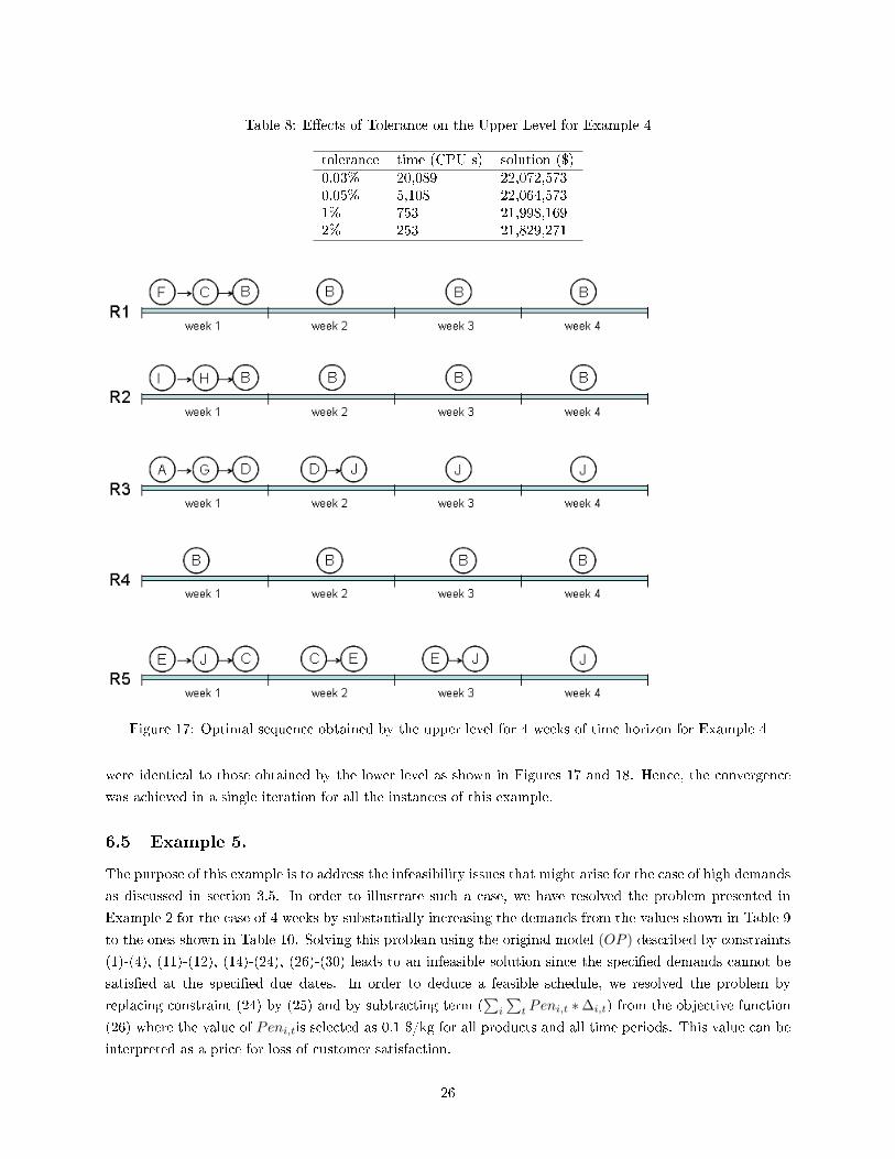
Table 8: E�ects of Tolerance on the Upper Level for Example 4

tolerance time (CPU s) solution ($)0.03% 20,089 22,072,5730.05% 5,108 22,064,5731% 753 21,998,1692% 253 21,829,271

Figure 17: Optimal sequence obtained by the upper level for 4 weeks of time horizon for Example 4

were identical to those obtained by the lower level as shown in Figures 17 and 18. Hence, the convergence

was achieved in a single iteration for all the instances of this example.

6.5 Example 5.

The purpose of this example is to address the infeasibility issues that might arise for the case of high demands

as discussed in section 3.5. In order to illustrate such a case, we have resolved the problem presented in

Example 2 for the case of 4 weeks by substantially increasing the demands from the values shown in Table 9

to the ones shown in Table 10. Solving this problem using the original model (OP ) described by constraints

(1)-(4), (11)-(12), (14)-(24), (26)-(30) leads to an infeasible solution since the speci�ed demands cannot be

satis�ed at the speci�ed due dates. In order to deduce a feasible schedule, we resolved the problem by

replacing constraint (24) by (25) and by subtracting term (∑i

∑t Peni,t ∗∆i,t) from the objective function

(26) where the value of Peni,tis selected as 0.1 $/kg for all products and all time periods. This value can be

interpreted as a price for loss of customer satisfaction.

26

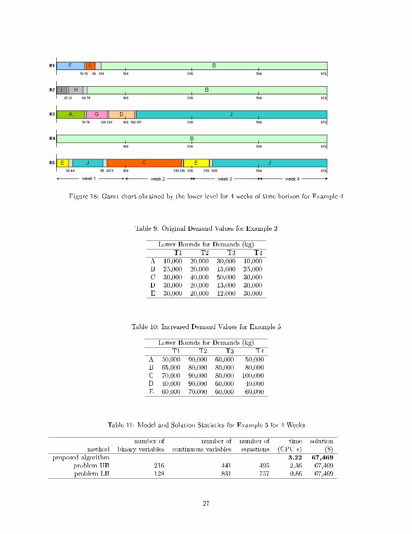
Figure 18: Gantt chart obtained by the lower level for 4 weeks of time horizon for Example 4

Table 9: Original Demand Values for Example 2

Lower Bounds for Demands (kg)T1 T2 T3 T4

A 10,000 20,000 30,000 10,000B 25,000 20,000 15,000 25,000C 30,000 40,000 50,000 30,000D 30,000 20,000 13,000 30,000E 30,000 20,000 12,000 30,000

Table 10: Increased Demand Values for Example 5

Lower Bounds for Demands (kg)T1 T2 T3 T4

A 50,000 90,000 60,000 50,000B 65,000 80,000 80,000 80,000C 70,000 90,000 80,000 100,000D 40,000 90,000 60,000 40,000E 60,000 70,000 60,000 60,000

Table 11: Model and Solution Statistics for Example 5 for 4 Weeks

number of number of number of time solutionmethod binary variables continuous variables equations (CPU s) ($)

proposed algorithm 3.22 67,469problem UB 216 441 495 2.36 67,469problem LB 128 831 757 0.86 67,469

27

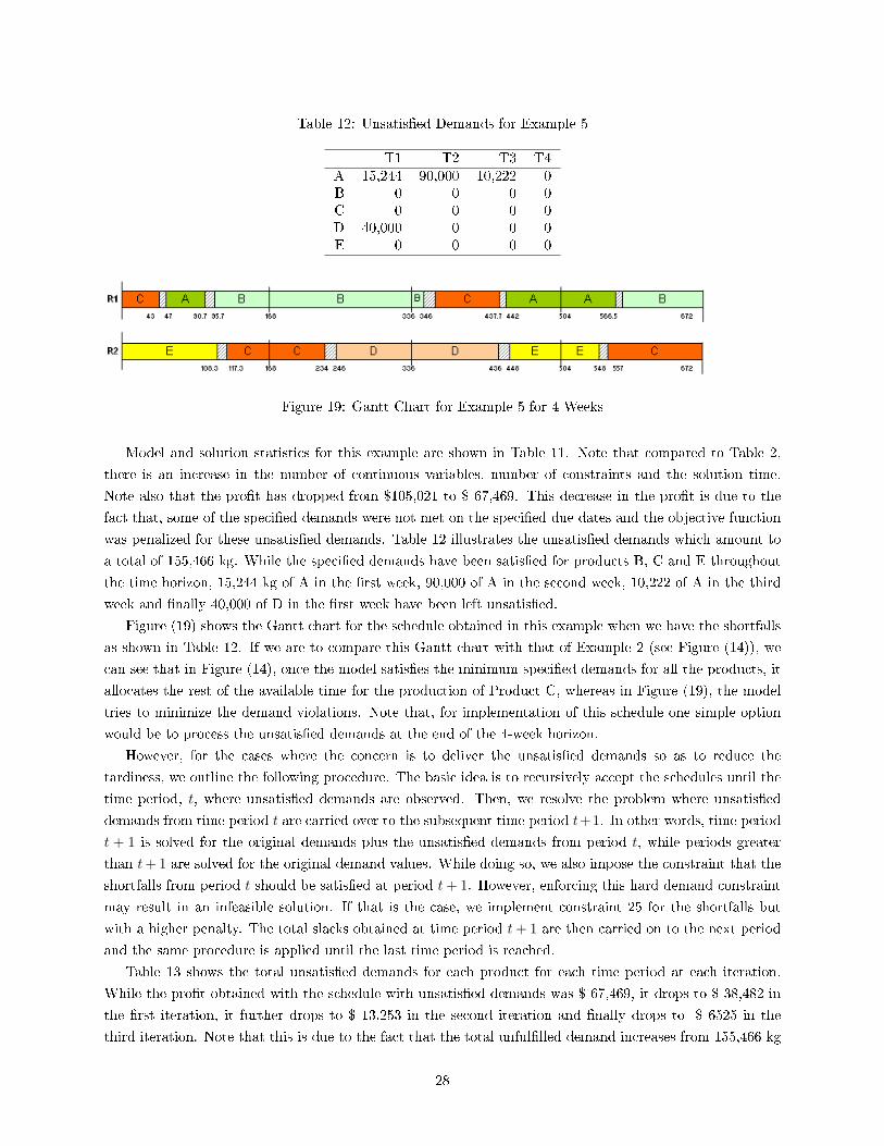
Table 12: Unsatis�ed Demands for Example 5

T1 T2 T3 T4A 15,244 90,000 10,222 0B 0 0 0 0C 0 0 0 0D 40,000 0 0 0E 0 0 0 0

Figure 19: Gantt Chart for Example 5 for 4 Weeks

Model and solution statistics for this example are shown in Table 11. Note that compared to Table 2,

there is an increase in the number of continuous variables, number of constraints and the solution time.

Note also that the pro�t has dropped from $105,021 to $ 67,469. This decrease in the pro�t is due to the

fact that, some of the speci�ed demands were not met on the speci�ed due dates and the objective function

was penalized for these unsatis�ed demands. Table 12 illustrates the unsatis�ed demands which amount to

a total of 155,466 kg. While the speci�ed demands have been satis�ed for products B, C and E throughout

the time horizon, 15,244 kg of A in the �rst week, 90,000 of A in the second week, 10,222 of A in the third

week and �nally 40,000 of D in the �rst week have been left unsatis�ed.

Figure (19) shows the Gantt chart for the schedule obtained in this example when we have the shortfalls

as shown in Table 12. If we are to compare this Gantt chart with that of Example 2 (see Figure (14)), we

can see that in Figure (14), once the model satis�es the minimum speci�ed demands for all the products, it

allocates the rest of the available time for the production of Product C, whereas in Figure (19), the model

tries to minimize the demand violations. Note that, for implementation of this schedule one simple option

would be to process the unsatis�ed demands at the end of the 4-week horizon.

However, for the cases where the concern is to deliver the unsatis�ed demands so as to reduce the

tardiness, we outline the following procedure. The basic idea is to recursively accept the schedules until the

time period, t, where unsatis�ed demands are observed. Then, we resolve the problem where unsatis�ed

demands from time period t are carried over to the subsequent time period t+1. In other words, time period

t + 1 is solved for the original demands plus the unsatis�ed demands from period t, while periods greater

than t+ 1 are solved for the original demand values. While doing so, we also impose the constraint that the

shortfalls from period t should be satis�ed at period t+ 1. However, enforcing this hard demand constraint

may result in an infeasible solution. If that is the case, we implement constraint 25 for the shortfalls but

with a higher penalty. The total slacks obtained at time period t+ 1 are then carried on to the next period

and the same procedure is applied until the last time period is reached.

Table 13 shows the total unsatis�ed demands for each product for each time period at each iteration.

While the pro�t obtained with the schedule with unsatis�ed demands was $ 67,469, it drops to $ 38,482 in

the �rst iteration, it further drops to $ 13,253 in the second iteration and �nally drops to -$ 6525 in the

third iteration. Note that this is due to the fact that the total unful�lled demand increases from 155,466 kg

28

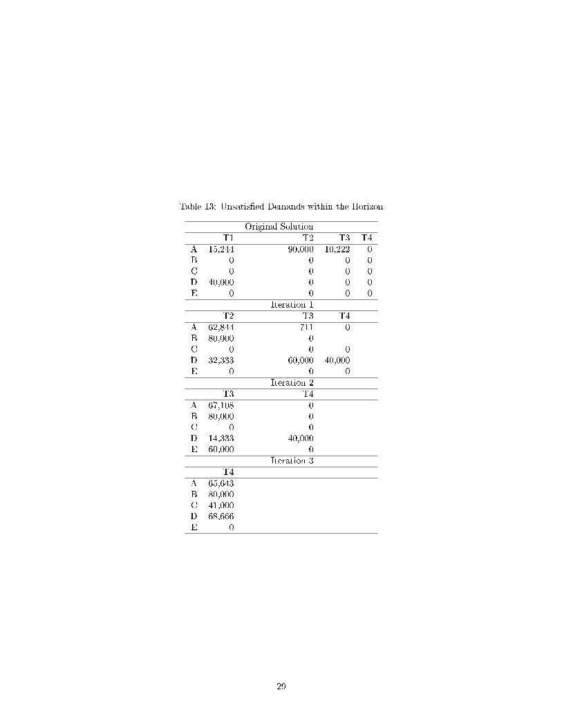
Table 13: Unsatis�ed Demands within the Horizon

Original SolutionT1 T2 T3 T4

A 15,244 90,000 10,222 0B 0 0 0 0C 0 0 0 0D 40,000 0 0 0E 0 0 0 0

Iteration 1T2 T3 T4

A 62,844 711 0B 80,000 0C 0 0 0D 32,333 60,000 40,000E 0 0 0

Iteration 2T3 T4

A 67,108 0B 80,000 0C 0 0D 14,333 40,000E 60,000 0

Iteration 3T4

A 65,643B 80,000C 41,000D 68,666E 0

29

(Table 12) where we minimize total violation, to 255,309 kg (Table 13) where we try to minimize tardiness.

7 Conclusions

We have addressed the simultaneous planning and scheduling of single stage continuous plants with parallel

units. We have presented a slot based MILP model, which is the extension of the work by Erdirik-Dogan

and Grossmann [2006] for single units to the case of multiple parallel units. While this model is e�ective

for small sized problems and short time horizons, the MILP model becomes computationally expensive to

solve for large problems with long time horizons. In order to address this problem we propose a bi-level

decomposition scheme. While the proposed decomposition approach is an extension of the work of Erdirik-

Dogan and Grossmann [2006], the di�erence lies on how the upper level model is de�ned. This model is

not only concerned with the assignments of products to units and time periods, but also with the e�ects

of sequencing. Accounting for the scheduling explicitly at the upper level made it possible to successfully

integrate planning and scheduling by obtaining very tight upper bounds.

The results show that the proposed upper level model yields signi�cant improvements over the previous

upper level model. Global optimal solutions are obtained by the upper level when there are no subcycles.

It is important to note that among all the instances we have solved so far, only one instance exhibited a

subcycle. Application of the proposed decomposition approach has proved to be very e�ective requiring

only a single iteration between the master and the subproblem for all the instances we have solved so far.

Therefore, compared to the full-space method, the proposed approach decreased the solution times by more

than an order of magnitude. However, we should point out that the upper level model is now the bottleneck

in computation due to the sequencing decisions incorporated at that level, which results in a rapid increase

in the computational time as increasing number of time periods. Therefore, the trade-o� between decreasing

the number of iterations by obtaining tight upper bounds and increasing the computational e�ort of solving

the problem should be investigated in future work.

Acknowledgments

The authors would like to acknowledge �nancial support from the Pennsylvania Infrastructure Technology

Alliance, Institute of Complex Engineered Systems, and from the National Science Foundation under Grant

No. DMI-0556090. We would like to thank Dr. Je�rey Kelly from Honeywell for bringing constraints (11)

and (12) to our attention.

8 Appendix

Appendix A:

Constraint (6) has |I|∗|I|∗|M |∗|L− 1|∗|T |−|I|∗|M |∗|L− 1|∗|T |number of constraints. Constraints (11) and(12) on the other hand lead to |I|∗|M |∗|L|∗|T |+|I|∗|M |∗|L− 1|∗|T |constraints. The di�erence between thesize of constraint (6) and constraints (11) and (12) is equal to |I| ∗ |M | ∗ |T | ∗ [|I| ∗ |L− 1| − 2 ∗ |L− 1| − |L|].If the number of postulated slots are set equal to the number of products, |I| = |L|, than we can replace

|L| with |I| which leads to |I| ∗ |M | ∗ |T | ∗ [|I| ∗ |I − 1| − 2 ∗ |I − 1| − |I|] which is equal to |I| ∗ |M | ∗ |T | ∗[|I|2 − 4 ∗ |I|+ 2

]. Therefore, constraint (6) will lead to larger number of constraints provided that the

cardinality of the product set, |I| is greater than or equal to 4.

30

Appendix B:

Sum constraint (6) over i to obtain∑i Zi,k,m,l,t ≥

∑iWi,m,l,t +

∑iWk,m,l+1,t −

∑i 1. By substituting (1),

this becomes:

∑i

Zi,k,m,l,t ≥ 1 +∑i

Wk,m,l+1,t −Nm (58)

Similarly, sum constraint (6) over k and replace∑kWk,m,l+1,t by 1 using constraint (1) to obtain

∑k

Zi,k,m,l,t ≥ 1 +∑k

Wi,m,l,t −Nm (59)

Since∑iWk,m,l+1,tin (58) is independent of i, it can be replaced by Nm ∗Wk,m,l+1,t, and similarly in

(59) we can replace∑kWi,m,l,t by Nm ∗Wi,m,l,t to obtain,

∑i

Zi,k,m,l,t ≥ Nm.(Wk,m,l+1,t − 1) + 1 (60)

∑k

Zi,k,m,l,t ≥ Nm.(Wi,m,l,t − 1) + 1 (61)

If Wk,m,l+1,t = 1 then the right hand side of (60) becomes 1. If Wk,m,l+1,t = 0 then the right hand

side of (60) becomes 1 −Nm. However, since Zi,k,m,l,t ≥ 0, the right hand side of (60) cannot be negative.

Therefore, (60) does not depend on Nm, and hence Nm can be reduced to 1.Same argument follows for (61).

Hence, (60) and (61) become;

∑i

Zi,k,m,l,t ≥Wk,m,l+1,t (62)

and

∑k

Zi,k,m,l,t ≥Wk,m,l,t (63)

By constraint (8), if Wk,m,l+1,t is zero then Zi,k,m,l,t must be zero. Also, by (62) and (8), if Wk,m,l+1,t

is 1, then Zi,k,m,l,t must be 1 since its upper bound is 1. Hence, the inequality in (62) can be replaced by

equality in (12). Following the same argument, we can replace the inequality in (63) by the equality in (11).

Thus, it follows that (6)-(8) and (11)-(12) are equivalent since the latter can be derived from (6)-(8) as

has been proved. To prove that (11)-(12) are at least as tight, we set Wi,m,l,t = 1/ |I(m)| and Wk,m,l,t =1/ |I(m)|so that (1) is satis�ed provided |I(m)| ≥ 2. Setting Zi,k,m,l,t = 0, (6)-(8) are satis�ed. However,

(11)-(12) are violated. Thus, the feasible space of (11)-(12) is contained in the feasible space of (6)-(8). Also,

since every point satis�ed by (11)-(12) must be feasible for (6)-(8) by the above derivation from (58) to (63),

it follows that (11)-(12) is at least as tight as (6)-(8).

9 Nomenclature

Indices

i, k products

31

l slots

m units

t time periods

t̄ last time period

l̄m last slot of unit m

Sets

I set of products

Im set of products that can be processed on unit m

L set of slots

Lm set of slots that belong to unit m

M set of units

Mi set of units that can process product i

Parameters

Ht duration of the tth time period

HTt time in terms of hours at the end of the tthtime period

Nm number of slots postulated for unit m

MRTi,mminimum run lengths

ri,m production rate of product i in unit m

τi,k,m transition time from product i to product k in unit m

INV Ii initial inventory of product i

di,t demand of product i at the end of period t

CPi,t selling price of product i in period t

CINVi,t inventory cost of product i in period t

COPi,t operating cost of product i in period t

CTRANSi,k,m transition cost of changing the production from product i to k in unit m

Peni,tpenalty cost for unsatis�ed demands

V ariables

Wi,m,l,t 0-1 variable to denote the assignment of product i to slot l of unit m during period t

Y OPi,m,t 0-1 variable to denote if product i is assigned unit m during period t

Y Pi,m,t 0-1 variable to denote the assignment of product i to unit m during period t

ZPi,k,m,t 0-1 variable to denote if product i precedes product k in unit m during time period t

ZZPi,k,m,t 0-1 variable to denote if the link between products i and k are broken

XFi,m,t 0-1 variable to denote if product i is the �rst product in unit m during period t

XLi,m,t 0-1 variable to denote if product i is the last product in unit m during period t

Θi,m,l,t production time of product i in slot l of unit m during period t

θ̃i,m,t production time of product i in unit m during period t

Xi,m,l,t amount of product i produced in slot l of unit m during period t

X̃i,m,t amount of product i produced in unit m during period t

∆i,t slack variable

Zi,k,m,l,t to denote if product i is followed by product k in slot l of unit m during period t

TRTi,k,m,t to denote if product i is followed by product k at the end of period t

Tem,l,t end time of slot l of unit m during period t

Tsm,l,t start time of slot l of unit m during time period t

32

INVi,t inventory level of product i at the end of time period t

INV Oi,t inventory level of product i at the end of period t after the demands are satis�ed

Areai,t over estimation of the area below the inventory time graph for product i at the end of period t

Si,t sales of product i at the end of period t

NYi,m,t total number of slots that are allocated for product i in unit m during period t

TRNPm,t total transition time for unit m within each time period

ZZZi,k,m,t transition variable denoting the changeovers across adjacent periods

References

A. Alle, L.G. Papageorgiou, and J..M. Pinto. A mathematical programming approach for cyclic production

and cleaning scheduling of multistage continuous plants. Computers and Chemical Engineering, 28(3):15,

2004.

E. Balas and R. Jeroslow. Canonical cuts on the unit hypercube. SIAM J. Appl. Math., 23(61):79, 1972.

M. H. Bassett, J. F. Pekny, and G. V. Reklaitis. Decomposition techniques for the solution of large-scale

scheduling problems. American Institute of Chemical Engineering Journal, 42(3373):3384, 1996.

D. B. Birewar and I. E. Grossmann. Simultaneous production planning and scheduling in multiproduct batch

plants. Industrial Engineering and Chemical Research, 29(570):580, 1990.

A. D. Dimitriadis, N. Shah, and C. C. Pantelides. Rtn-based rolling horizon algorithms for medium term

scheduling of multipurpose plants. Computers and Chemical Engineering, 21(1061):1066, 1997.

M. Erdirik-Dogan and I. E. Grossmann. Optimal production planning models for parallel batch reactors

with sequence-dependent changeovers. to appear in American Institute of Chemical Engineering Journal,

submitted 2007.

M. Erdirik-Dogan and I.E. Grossmann. A decomposition method for the simultaneous planning and schedul-

ing of single-stage continuous multiproduct plants. Industrial Engineering and Chemical Research, 45(299),

2006.

V. Jain and I. E. Grossmann. Cyclic scheduling of continuous parallel process units with decaying perfor-

mance. American Institute of Chemical Engineering Journal, 44(1623):1636, 1998.

Z. Jia and M. Ierapetritou. E�cient short-term scheduling of re�nery operations based on a continuous time

formulation. Computers and Chemical Engineering, 20(1001):1019, 2004.

E. Kondili, C. C. Pantelides, and R. W. H. Sargent. A general algorihm for short term scheduling of batch

operations 1. milp formulation. Computers and Chemical Engineering, 17(211):227, 1993.

H. Lee, Pinto J. M., I. E. Grossmann, and S. Park. Mixed-integer linear programming model for re�nery

short-term scheduling of crude-oil unloading with inventory management. Industrial Engineering and

Chemical Research, 35(1639), 1996.

C.A. Mendez and J. Cerda. An e�cient milp continuous-time formulation for short-term scheduling of

multiproduct continuous facilities. Computers and Chemical Engineering, 26(687):695, 2002.

33

D. L. Miller and J. F. Pekny. Exact solution of large asymmetric traveling salesman problems. Science, 251

(754):761, 1991.

G. Nemhauser and L. Wolsey. Integer and Combinatorial Optimization. John Wiley and Sons, 1998.

C. C. Pantelides. Uni�ed frameworks for the optimal process planning and scheduling. In Proceedings of the

Second Conference on Foundations of Computer-Aided Process Operations, Vol. 1 CACHE: Austin, TX

(253):274, 1994.

L. G. Papageorgiou and C. C. Pantelides. Optimal campaign planning/scheduling of multipurpose

batch/semi-continuous plants, 2. a mathematical decomposition approach. Industrial Engineering and

Chemical Research, 35(510), 1996b.

J. M. Pinto and I. E. Grossmann. Optimal cyclic scheduling of multistage continuous multiproduct plants.

Computers and Chemical Engineering, 18(797):816, 1994.

N. V. Sahinidis and I. E. Grossmann. Minlp model for cyclic multiproduct scheduling on continuous parallel

lines. Computers and Chemical Engineering, 15(85):1036, 1991.

N. Shah. Mathematical programming techinques for crude-oil scheduling. Computers and Chemical Engi-

neering, 20(S1227), 1996.

C. Sung and C.T. Maravelias. An attainable region approach for production planning of multiproduct

processes. American Institute of Chemical Engineering Journal, 53(1298):1315, 2007.

S. J. Wilkinson, N. Shah, and C. C. Pantelides. Aggregate modeling of multipurpose plant operation.

Computers and Chemical Engineering, 19 (Supplement 1,11)(583):588, 1996.

34