simultaneously high gravimetric and volumetric gas · pdf files1 simultaneously high...

S1

Simultaneously High Gravimetric and Volumetric Gas Uptake

Characteristics of the Metal–Organic Framework NU-111

Yang Peng,

a,b Gadipelli Srinivas

a,b, Christopher E. Wilmer,

c Ibrahim Eryazici,

d Randall Q. Snurr,

c

Joseph T. Huppd, Taner Yildirim,

a,b,* and Omar K. Farha

d,*

Institutions:

aNIST Center for Neutron Research, National Institute of Standards and Technology, Gaithersburg,

Maryland, 20899-6102 (USA). bDepartment of Materials Science and Engineering, University of Pennsylvania, Philadelphia,

Pennsylvania, 19104-6272 (USA). cDepartment of Chemical and Biological Engineering, Northwestern University, 2145 Sheridan Road,

Evanston, Illinois 60208 (USA). dDepartment of Chemistry and International Institute for Nanotechnology, Northwestern University,

2145 Sheridan Road, Evanston, Illinois 60208 (USA).

* Corresponding authors: [email protected] and [email protected]

Table of Contents

Section S1. Linkers Used in 2nd

Generation MOFs with Very Large Surface Area S2

Section S2. Nitrogen Isotherms S3

Section S3. Volumetric High-Pressure Adsorption Measurements and Excess Isotherms on NU-111 S4-S7

Section S4. Measured Isosteric Heat of Adsorption Qst S8-S10

Section S5. Simulated High-Pressure Adsorption of NU-111 S11–S13

Section S6. X-ray pattern and crystal structure of NU-111 S13-15

Section S7. References S15

Electronic Supplementary Material (ESI) for Chemical CommunicationsThis journal is © The Royal Society of Chemistry 2013

mailto:[email protected]

S2

Section S1. Linkers Used in 2nd

Generation MOFs with Very Large Surface Area

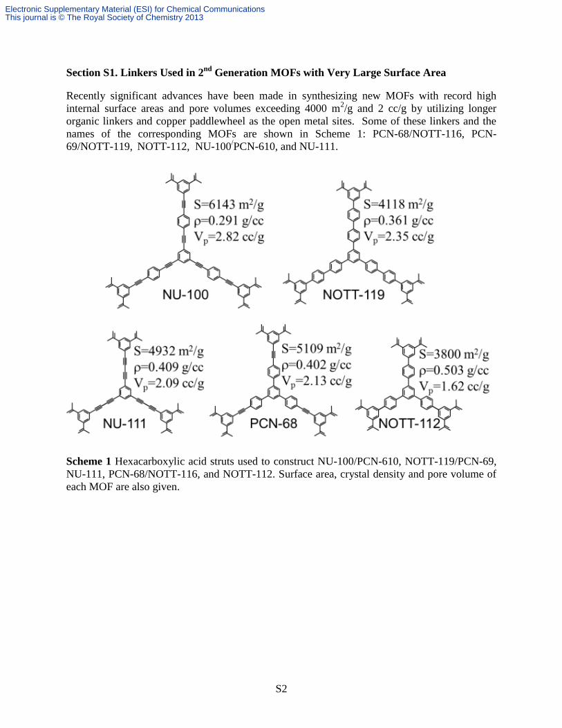
Recently significant advances have been made in synthesizing new MOFs with record high

internal surface areas and pore volumes exceeding 4000 m2/g and 2 cc/g by utilizing longer

organic linkers and copper paddlewheel as the open metal sites. Some of these linkers and the

names of the corresponding MOFs are shown in Scheme 1: PCN-68/NOTT-116, PCN-

69/NOTT-119, NOTT-112, NU-100

/PCN-610, and NU-111.

Scheme 1 Hexacarboxylic acid struts used to construct NU-100/PCN-610, NOTT-119/PCN-69,

NU-111, PCN-68/NOTT-116, and NOTT-112. Surface area, crystal density and pore volume of

each MOF are also given.


S3

Section S2. Nitrogen Isotherms

First, we studied the permanent porosity of activated NU-111 by N2 adsorption measurements at

77 K (Figure S1). By applying the Brunauer-Emmett-Teller (BET) model in the pressure range

P/P0 = 0.02 ~ 0.14, the specific surface area of NU-111 was calculated to be 4930 m2/g (see inset

in Figure S1), which agrees well with the value obtained from a simulated N2 isotherm of 4915

m2/g. This is one of the few MOFs with a BET surface area exceeding 3800 m

2/g. NU-111

exhibits exceptionally high N2 uptake of 1350 cc/g at saturation and a pore volume based on the

maximum of N2 adsorption of 2.09 cc/g. The experimental pore volume is in excellent agreement

with the value calculated from PLATON (2.03 cc/g).

Figure S1. N2 adsorption isotherm at 77 K. The inset on the left shows the consistency plot to

determine the pressure range for BET fitting2, which is shown in the right inset.


S4

Section S3. Volumetric High-Pressure Adsorption Measurements and Excess Isotherms on

NU-111.

Based on the widely used volumetric method, we developed a fully computer-controlled Sieverts

apparatus as discussed in detail in Ref. 1. Briefly, our fully computer controlled Sievert

apparatus operates in a sample temperature range of 20 K to 500 K and a pressure range of 0 to

100 bar. In the volumetric method, gas is admitted from a dosing cell with known volume to the

sample cell in a controlled manner; the gas pressure and temperature are controlled and recorded.

Some unique features of our setup are as follows. We have five gas inlets including He, N2, CO2,

CH4, and H2, enabling us to perform first nitrogen pore volume and surface measurements and

then He-cold volume determination and then the gas adsorption measurements without moving

the sample from the cell and using the same protocol. We use four pressure gauges with four

different pressure ranges (20, 100, 500 and 3000 psi respectively) to precisely measure the

pressure. For isotherm measurement below room temperature, the sample temperature is

controlled using a closed cycle refrigerator (CCR). The difference between the real sample

temperature and the control set-point is within 1 K in the whole operating temperature range. The

connection between the sample cell and the dose cell is through 1/8’’ capillary tubing, which

provides a sharp temperature interface between the sample temperature and the dose temperature

(i.e., room temperature).

The cold volumes for the empty cell were determined using He as a function of pressure at every

temperature before the real sample measurement and were used to calculate the sample

adsorption. In parallel to these empty cell based isotherms, we also measured isotherms using

He gas and sample in the cell. Assuming He-adsorption is small, this method is more accurate.

As shown in the Figure below, the isotherms from both methods (i.e. empty cell cold volume,

and He-cold volume with the sample) agree with each other reasonably well. As a third cross

check of our measurements, we repeated all the isotherms on an empty cell with the same gas

and temperatures. Using previously measured cold volumes, we verify that the empty cell does

not appear to show any adsorption. Based on this empty cell absorption measurement, the error

bars in our isotherms are around 1% at 35 bar and at most 2-3 % at 60 bar.

In the paper (and below), we compare the absolute (and excess) isotherms obtained from He-runs

(orange color) and the blank empty cell runs (black). For practical purposes, the two methods

result in basically very similar isotherms, giving us confidence about the measurements and

some idea about the error bars. The biggest difference is at 200 and 240 K where He-runs give

lower isotherms. This is what we expect. At these temperatures and at high pressures, some He

will be adsorbed in the sample, which results in a slightly larger cold-volume and therefore lower

adsorption. At high temperatures, He-runs seem to give slightly higher isotherms than empty

cell runs. The difference is about 1-3 percent.

Since the adsorbed amount is deducted from the raw P-V-T data using a real gas equation of

state, a critically important issue is the accuracy of the chosen equation of state (EOS) in terms of

describing the real gas behavior within the desired temperature and pressure range. We found

that the simple EOS such as van der Waals (vdW) EOS works well at only ambient pressure and

temperature, while it cannot describe the real gas behavior at low temperature and high pressure.

Alternatively, for small gas molecules, the modified Benedict-Webb-Rubin (MBWR) EOS


S5

seems to work well over a wide temperature and pressure range. Using an empty cell as a

reference, we found that the MBWR EOS best describes the real gas behavior of He, H2 and

CH4. Therefore, in all our isotherm data reduction, the NIST MBWR EOS is used. [NIST

Standard Reference Database 23: NIST Reference Fluid Thermodynamic and Transport

Properties Database].

Finally, we note that we repeated both CH4 and CO2 isotherms at room temperature several

times over a period of six months and did not see any evidence of sample degradation. We

believe that as long as the sample is kept in an inert atmosphere such as in He-glove box, it is

very stable and many cycles of adsorption of CO2/CH4 do not seem to have any effect on the

adsorption uptake capacity.

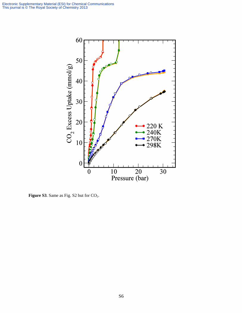
Figure S2. The excess isotherms for CH4 at various temperatures. The corresponding total isotherms are

shown and discussed in the text. The total (i.e. absolute) isotherms were obtained from excess isotherms

by adding the amount of gas in the pore volume at the measured pressure and temperature (using the

NIST MBWR real gas equation). We used the measured pore volume from the nitrogen isotherm. The

orange color lines represent isotherms obtained from He-cold volume with sample in while the other

isotherms are using empty-cell vold volumes. The difference is due to adsorption of He by the sample.

Open symbols indicate desorption isotherms.


S6

Figure S3. Same as Fig. S2 but for CO2.


S7

Figure S4. Excess isotherms for H2 at various temperatures.


S8

Section S4. Measured Isosteric Heat of Adsorption Qst

Our isotherm data at a series of temperatures (Fig. 2 of the main text) enable us to extract the

heat of adsorption Qst as a function of the adsorbed amount. Qst is calculated using the “isosteric

method” where a series of isotherms are measured at a wide range of temperatures. These

isotherms are then parameterized by cubic-spline which does not require any fitting and allows

us to interpolate the isotherm at a constant loading. Then, the Qst is obtained from the ln(P)

versus 1/T plots. As an alternative to cubic-spline interpolation, we also obtain Qst by fitting the

isotherm data using the following form of a virial equation:

( ) ( )

∑

∑

where v, p, and T are the amount adsorbed, pressure, and temperature, respectively and ai and bi

are empirical parameters. The first four constants (i.e. a0, b0, a1, and b1) are obtained by

linearizing the isotherms (1/n versus ln p) and then we increase the number of parameters

gradually (two at a time) until the improvement in the fit is not significant. Usually 10 or 12

parameters are found to be enough to obtain a good fit to the isotherms. After the isotherms are

fitted, by applying Clausius-Clapeyron equation, the heat of adsorption is obtained as

∑

where R is the universal gas constant. The details can be found in [Jagiello et al, J. Chem. Eng.

Data, 1995; 40; 1288-92 and Jagiello J at al, Langmuir 1996, 12,2837-42].

Figure S5. Isosteric heats of adsorption for H2, CH4 and CO2. The red and black lines are from

experimental data using spline and virial fitting, respectively. The blue dashed lines represent Qst

values determined from the simulated isotherms.


S9

As an example, below we show the isotherm data (points), cubic-spline interpolation (solid lines)

and the virial-fit (dotted lines) as well as the corresponding ln(P) versus 1/T plots and the Qst

from both methods along with the fit parameters ai and bi.

Figure S6. The H2 adsorption isotherms (dots) and the virial fit (red-lines) along with the fit parameters as well as

the Qst and the lnP-1/T plots. The black line in the Qst plot is obtained from the raw-data without any virial fitting

(using spline method).


S10

Figure S7. Same as Fig. S6 but for CH4 adsorption.

Figure S8. Same as Fig. S6 but for CO2 adsorption.


S11

Section S5. Simulated High-Pressure Adsorption of NU-111

Atomistic grand canonical Monte Carlo (GCMC) simulations were performed to estimate the

adsorption isotherms of N2, CH4, CO2 and H2 in NU-111.

Interaction potential. For simulations of N2, CH4, and CO2 adsorption, interaction energies

between non-bonded atoms were computed through a Lennard-Jones (LJ) + Coulomb potential:

((

)

(

)

)

where i and j are interacting atoms, and is the distance between atoms i and j, and are

the LJ well depth and diameter, respectively, and are the partial charges of the interacting

atoms, and is the dielectric constant. LJ parameters between different types of sites were

calculated using the Lorentz-Berthelot mixing rules.

For simulations of H2 adsorption at 77 K, quantum diffraction effects become important, which

can be accounted for using the quasiclassical Feynman-Hibbs (FH) potential.3,4

We modeled

hydrogen at this temperature as follows:

((

)

(

)

)

( (

)

(

)

)

⏞ orrection

where is the reduced mass, ( ) of the two interacting atoms having atomic

masses and , is the temperature, and and are Boltzmann’s constant and Planck’s

constant, respectively. For comparison, we also ran simulations without the middle Feynman-

ibbs “correction” term.

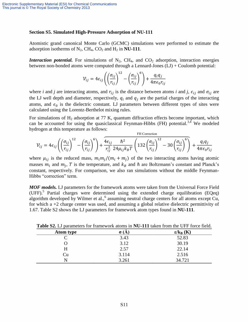
MOF models. LJ parameters for the framework atoms were taken from the Universal Force Field

(UFF).5 Partial charges were determined using the extended charge equilibration (EQeq)

algorithm developed by Wilmer et al.,6 assuming neutral charge centers for all atoms except Cu,

for which a +2 charge center was used, and assuming a global relative dielectric permittivity of

1.67. Table S2 shows the LJ parameters for framework atom types found in NU-111.

Table S2. LJ parameters for framework atoms in NU-111 taken from the UFF force field.

Atom type σ (Å) ε/kB (K)

C 3.43 52.83

O 3.12 30.19

H 2.57 22.14

Cu 3.114 2.516

N 3.261 34.721


S12

Nitrogen Model. Nitrogen molecules were modeled using the TraPPE force field,7 which was

originally fit to reproduce the vapor-liquid coexistence curve of nitrogen. In this force field, the

nitrogen molecule is a rigid structure where the N-N bond length is fixed at its experimental

value of 1.10 Å. This model reproduces the experimental gas-phase quadrupole moment of

nitrogen by placing partial charges on N atoms and on a point located at the center of mass

(COM) of the molecule. Table S3 shows the LJ parameters and partial charges for nitrogen.

Table S3. LJ parameters and partial charges for the sites in the nitrogen molecule.

Atom type σ (Å) ε/kB (K) q (e)

N 3.31 36.0 -0.482

N2 COM 0 0 0.964

Methane model. The methane molecules were modeled using the TraPPE force field,8 which

was originally fit to reproduce the vapor-liquid coexistence curve of methane. In this force field,

methane is modeled as a single sphere with the parameters shown in Table S5.

Table S4. LJ parameters for methane molecules.


CH4 (united) 3.75 148.0 ---

Carbon dioxide model. Partial charges and LJ parameters for CO2 were taken from the TraPPE

force field.7 This force field has been fit to reproduce the vapor-liquid coexistence curves by

Siepmann and co-workers. The CO2 molecule is modeled as a rigid and linear structure. Table S5

shows the LJ parameters and partial charges for CO2.

Table S5. LJ parameters and partial charges for the sites in the carbon dioxide molecule.


C 2.80 27.0 0.70

O 3.05 79.0 -0.35

Hydrogen Model. For the hydrogen molecules, we used the model of Levesque et al.9 and ran

simulations with the FH correction. In this model, the hydrogen molecule is a rigid structure

where the H-H bond length is fixed at 0.74 Å. This model reproduces the experimental gas-phase

quadrupole moment of hydrogen by placing partial charges on H atoms and on a point located at

the center of mass (COM) of the hydrogen molecule. Table S6 shows the LJ parameters and

partial charges for hydrogen.

Table S6. LJ parameters and partial charges for the sites in the hydrogen molecule.


H 0 0 0.468

H2 COM 2.958 36.7 -0.936

General GCMC simulation settings. All GCMC simulations included a 2500-cycle equilibration

period followed by a 2500-cycle production run. A cycle consists of n Monte Carlo steps, where

n is equal to the number of molecules (which fluctuates during a GCMC simulation). All


S13

simulations included random insertion/deletion, translation and rotation moves (except methane,

where no rotation moves were used) of molecules with equal probabilities. Atoms in the MOF

were held fixed at their crystallographic positions. An LJ cutoff distance of 12.0 Å was used for

all simulations. The Ewald sum technique was used to compute the electrostatic interactions.

One unit cell of NU-111 was used for the simulations. N2 isotherms were simulated at 77 K up to

0.398 bar. Fugacities needed to run the GCMC simulations were calculated using the Peng-

Robinson equation of state.

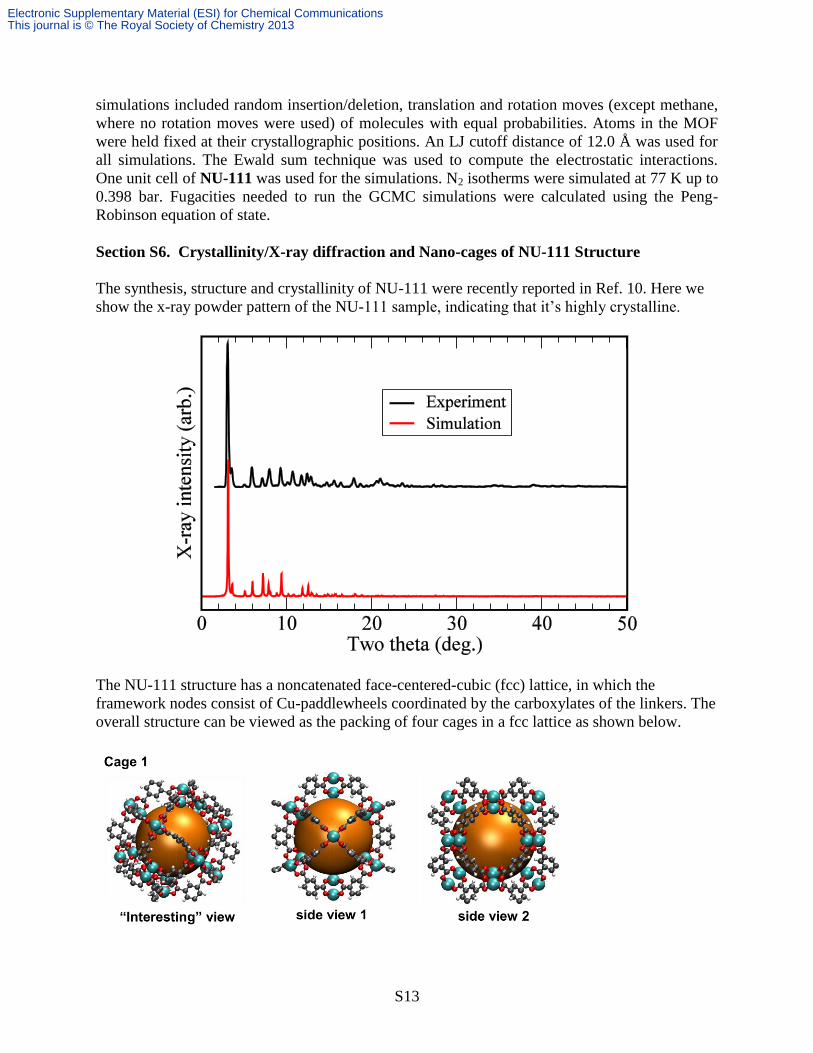
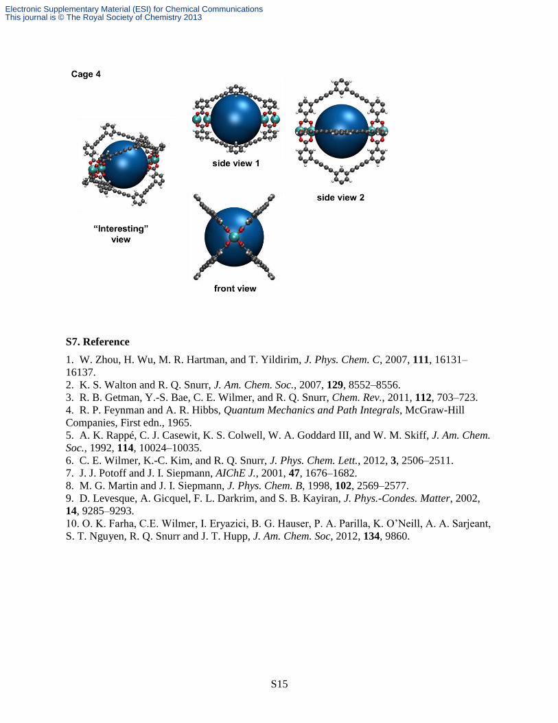
Section S6. Crystallinity/X-ray diffraction and Nano-cages of NU-111 Structure

The synthesis, structure and crystallinity of NU-111 were recently reported in Ref. 10. Here we

show the x-ray powder pattern of the NU-111 sample, indicating that it’s highly crystalline.

The NU-111 structure has a noncatenated face-centered-cubic (fcc) lattice, in which the

framework nodes consist of Cu-paddlewheels coordinated by the carboxylates of the linkers. The

overall structure can be viewed as the packing of four cages in a fcc lattice as shown below.


S14


S15

S7. Reference

1. W. Zhou, H. Wu, M. R. Hartman, and T. Yildirim, J. Phys. Chem. C, 2007, 111, 16131–

16137.

2. K. S. Walton and R. Q. Snurr, J. Am. Chem. Soc., 2007, 129, 8552–8556.

3. R. B. Getman, Y.-S. Bae, C. E. Wilmer, and R. Q. Snurr, Chem. Rev., 2011, 112, 703–723.

4. R. P. Feynman and A. R. Hibbs, Quantum Mechanics and Path Integrals, McGraw-Hill

Companies, First edn., 1965.

5. A. K. Rappé, C. J. Casewit, K. S. Colwell, W. A. Goddard III, and W. M. Skiff, J. Am. Chem.

Soc., 1992, 114, 10024–10035.

6. C. E. Wilmer, K.-C. Kim, and R. Q. Snurr, J. Phys. Chem. Lett., 2012, 3, 2506–2511.

7. J. J. Potoff and J. I. Siepmann, AIChE J., 2001, 47, 1676–1682.

8. M. G. Martin and J. I. Siepmann, J. Phys. Chem. B, 1998, 102, 2569–2577.

9. D. Levesque, A. Gicquel, F. L. Darkrim, and S. B. Kayiran, J. Phys.-Condes. Matter, 2002,

14, 9285–9293.

10. O. K. arha, .E. Wilmer, I. Eryazici, B. G. auser, P. A. Parilla, K. O’Neill, A. A. Sarjeant,

S. T. Nguyen, R. Q. Snurr and J. T. Hupp, J. Am. Chem. Soc, 2012, 134, 9860.


simultaneously high gravimetric and volumetric gas · pdf files1 simultaneously high...

Documents