single-cell rna-seq data analysis using chipster
TRANSCRIPT

CSC – Suomalainen tutkimuksen, koulutuksen, kulttuurin ja julkishallinnon ICT-osaamiskeskus
Single-cell RNA-seq data analysisusing Chipster
9.2.2018
Understanding data analysis - why?
• Bioinformaticians might not always be available when needed
• Biologists know their own experiments best
oBiology involved (e.g. genes, pathways, etc)
oPotential batch effects etc
• Allows you to design experiments better less money wasted
• Allows you to discuss more easily with bioinformaticians
8.2.20182

What will I learn?
• How to operate the Chipster software
• Analysis of single cell RNA-seq data
o Central concepts
o Analysis steps
o File formats
• Exercises
o DropSeq data preprocessing (from raw reads to expression values)
o Clustering analysis of 10X Genomics data with Seurat tools
8.2.20183

Introduction to Chipster

• Provides an easy access to over 360 analysis tools
o Command line tools
o R/Bioconductor packages
• Free, open source software
• What can I do with Chipster?
o analyze and integrate high-throughput data
o visualize data efficiently
o share analysis sessions
o save and share automatic workflows
Chipster

Technical aspects
• Client-server system
o Enough CPU and memory for large analysis jobsoCentralized maintenance
• Easy to install
oClient uses Java Web Starto Server available as a virtual machine


Mode of operationSelect: data tool category tool run visualize

Job manager
• You can run many analysis jobs at the same time
• Use Job manager to:
o view status
o cancel jobs
o view time
o view parameters

Analysis history is saved automatically -you can add tool source code to reports if needed

Analysis sessions
• Remember to save the analysis session.
oSession includes all the files, their relationships and metadata (what tool and parameters were used to produce each file).
oSession is a single .zip file.
• You can save a session locally (on your computer)
• and in the cloud
obut note that the cloud sessions are not stored forever!
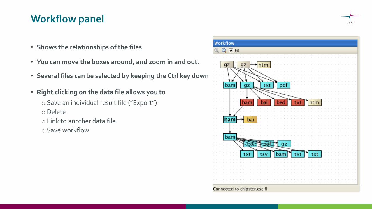
Workflow panel
• Shows the relationships of the files
• You can move the boxes around, and zoom in and out.
• Several files can be selected by keeping the Ctrl key down
• Right clicking on the data file allows you to
o Save an individual result file (”Export”)
oDelete
o Link to another data file
o Save workflow

Workflow – reusing and sharing your analysis pipeline
• You can save your analysis steps as a reusable automatic ”macro”
oall the analysis steps and their parameters are saved as a script file
oyou can apply workflow to another dataset
oyou can share workflows with other users

Saving and using workflows
• Select the starting point for your workflow
• Select ”Workflow / Save starting from selected”
• Save the workflow file on your computer with a
meaningful name
oDon’t change the ending (.bsh)!
• To run a workflow, select
oWorkflow -> Open and run
oWorkflow -> Run recent (if you saved the workflow recently).

Analysis tool overview
• 160 NGS tools for
RNA-seq
single cell RNA-seq
small RNA-seq
exome/genome-seq
ChIP-seq
FAIRE/DNase-seq
CNA-seq
Metagenomics (16S rRNA)
• 140 microarray tools for
gene expression
miRNA expression
protein expression
aCGH
SNP
integration of different data
• 60 tools for sequence analysis
BLAST, EMBOSS, MAFFT
Phylip

Visualizing the data
• Data visualization panel
o Maximize and redraw for better viewing
o Detach = open in a separate window, allows you to view several images at the same time
• Two types of visualizations
1. Interactive visualizations produced by the client program
o Select the visualization method from the pulldown menu
o Save by right clicking on the image
2. Static images produced by analysis tools
o Select from Analysis tools / Visualisation
o View by double clicking on the image file
o Save by right clicking on the file name and choosing ”Export”

Interactive visualizations by the client• Genome browser
• Spreadsheet
• Histogram
• Venn diagram
• Scatterplot
• 3D scatterplot
• Volcano plot
• Expression profiles
• Clustered profiles
• Hierarchical clustering
• SOM clustering
Available actions:
• Select genes and create a gene list
• Change titles, colors etc
• Zoom in/out

Static images produced by R/Bioconductor
• Dispersion plot
• MA plot
• MDS plot
• Box plot
• Histogram
• Heatmap
• tSNE plot
• Violin plot
• PCA plot
• Dendrogram
• K-means clustering
• SOM-clustering
• Etc…

Options for importing data to Chipster
• Import files/ Import folder
• Import from URL
oUtilities / Download file from URL directly to server
• Open an analysis session
oFiles / Open session
• Import from SRA database
oUtilities / Retrieve FASTQ or BAM files from SRA
• Import from Ensembl database
oUtilities / Retrieve data for a given organism in Ensembl
• What kind of RNA-seq data files can I use in Chipster?
oCompressed files (.gz) and tar packages (.tar) are ok
oFASTQ, BAM, read count files (.tsv), GTF
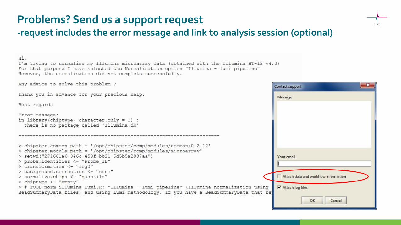
Problems? Send us a support request -request includes the error message and link to analysis session (optional)

Chipster Web version


Acknowledgements to Chipster users and contibutors

Introduction to single cell RNA-seq

Single cell RNA-seq
• New technology, data analysis methods are actively developed
• Measures distribution of expression levels for each gene across a population of cells
• Allows to study cell-specific changes in transciptome
• Applications
o Identifying cell sub-populations within a biological condition
oStudying dynamic processes like differentiation using pseudotime ordering
o Swithces
oBranch points
oTranscriptional regulatory networks
• Datasets range from 102 to 105 cells
8.2.201827

Single cell RNA-seq technology
• Protocols:
oDropSeq
o InDrop
oCELL-seq
oSMART-seq
oSMARTer
oMARS-seq
oSCRB-seq
oSeq-well
oSTRT-seq
• Commercial platforms:
oFluidigm C1 (FuGU)
o10x Genomics Chromium (FIMM, BTK)
8.2.201828

8.2.201829 https://hemberg-lab.github.io/scRNA.seq.course/introduction-to-single-cell-rna-seq.html


DropSeq data preprocessing overview
8.2.201831
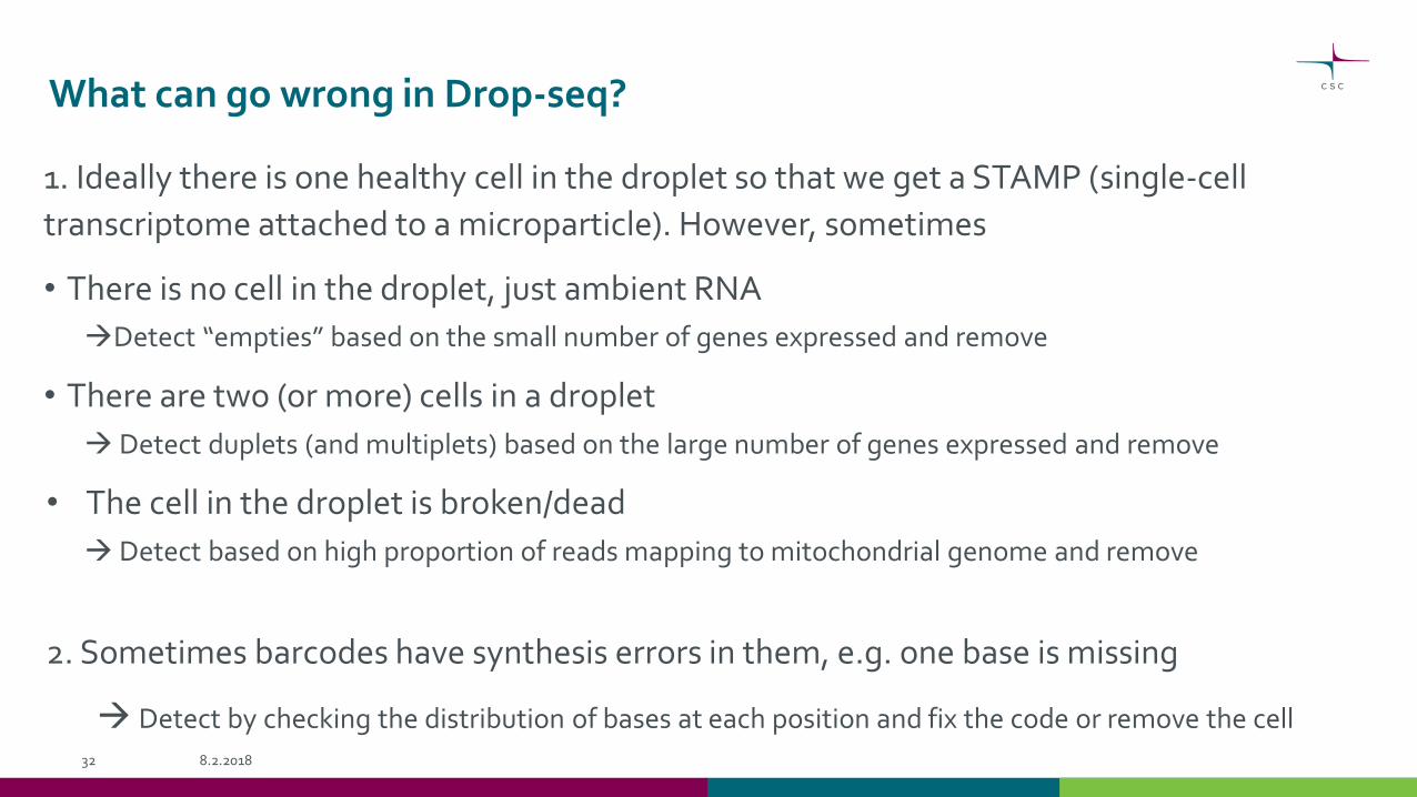
What can go wrong in Drop-seq?
1. Ideally there is one healthy cell in the droplet so that we get a STAMP (single-cell
transcriptome attached to a microparticle). However, sometimes
• There is no cell in the droplet, just ambient RNA
Detect “empties” based on the small number of genes expressed and remove
• There are two (or more) cells in a droplet
Detect duplets (and multiplets) based on the large number of genes expressed and remove
• The cell in the droplet is broken/dead
Detect based on high proportion of reads mapping to mitochondrial genome and remove
2. Sometimes barcodes have synthesis errors in them, e.g. one base is missing
Detect by checking the distribution of bases at each position and fix the code or remove the cell
8.2.201832

Single cell RNA-seq data analysis

Single cell RNA-seq data is challenging
• The detected expression level for many genes is zero
• Data is noisy. High level of variation due to
oCapture efficiency (percentage of mRNAs captured)
oAmplification bias (non-uniform amplification of transcripts)
oCells differ in terms of cell-cycle stage and size
• Complex distribution of expression values
oCell heterogeneity and the abundance of zeros give rise to multimodal distributions
Many methods used for bulk RNA-seq data won’t work
8.2.201834

scRNA-seq data analysis steps
8.2.201836
QC of raw reads
Preprocessing
Alignment
Annotation
Read count (DGE matrix)
Differential expression
Clustering

DropSeq data preprocessing

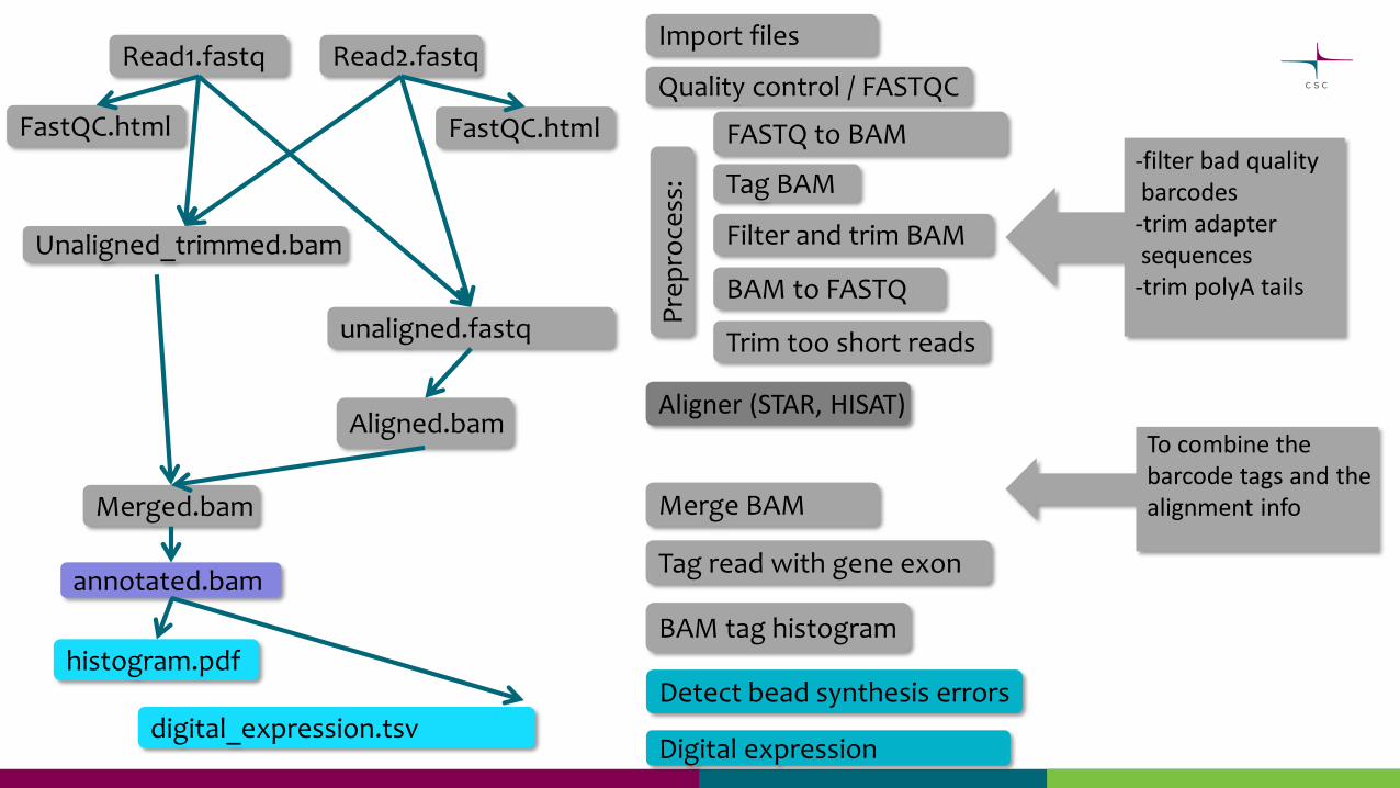
From FASTQ to expression matrix –preprocessing of DropSeq data
• Quality control of raw reads
• Preprocessing: tagging with barcodes & filtering
• Alignment to reference genome
• Merge BAM files
• Annotate with gene names
• Estimate the number of usable cells
• Detect bead synthesis errors
• Generate digital expression matrix
8.2.201838

Read1.fastq Read2.fastq
Unaligned_trimmed.bam
Import files
unaligned.fastq
Aligned.bam Aligner (STAR, HISAT)
Merged.bam Merge BAM
annotated.bamTag read with gene names
+ Detect bead synthesis errors
histogram.pdf
digital_expression.tsv
Estimate number of usable cells
Create digital expression matrix
-filter bad qualitybarcodes
-trim adapter sequences
-trim polyA tails
Combines thebarcode tags and the alignment info
Pre
pro
cess
:
FASTQ to BAM
Tag BAM
Filter and trim BAM
BAM to FASTQ
Filter too short reads
FastQC.html FastQC.html
Quality control / FASTQC

From FASTQ to expression matrix –preprocessing of DropSeq data
• Quality control of raw reads
• Preprocessing: tagging with barcodes & filtering
• Alignment to reference genome
• Merge BAM files
• Annotate with gene names
• Estimate the number of usable cells
• Detect bead synthesis errors
• Generate digital expression matrix
8.2.201840

What and why?
Potential problemso low confidence bases, Ns
osequence specific bias, GC bias
oadapters
osequence contamination
ounexpected length of reads
o…
Knowing about potential problems in your data allows you toocorrect for them before you spend a lot of time on analysis
otake them into account when interpreting results

Software packages for quality control
• FastQC
• FastX
• PRINSEQ
• TagCleaner
• ...

Raw reads: FASTQ file format
• Four lines per read:
@read name
GATTTGGGGTTCAAAGCAGTATCGATCAAATAGTAAATCCATTTGTTCAACTCACAGTTT
+ read name
!''*((((***+))%%%++)(%%%%).1***-+*''))**55CCF>>>>>>CCCCCCC65
• http://en.wikipedia.org/wiki/FASTQ_format
• Attention: Do not unzip FASTQ files!
oChipster’s analysis tools can cope with zipped files (.gz)
Base qualities
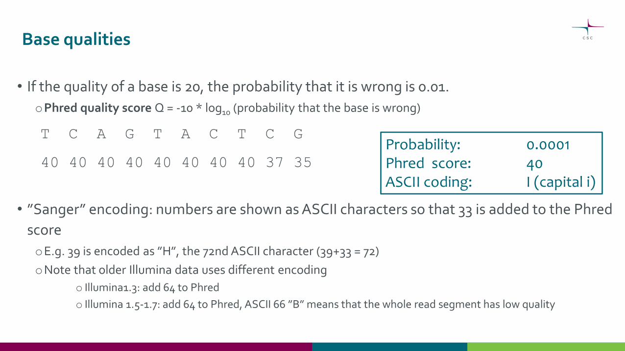
• If the quality of a base is 20, the probability that it is wrong is 0.01.
oPhred quality score Q = -10 * log10 (probability that the base is wrong)
T C A G T A C T C G
40 40 40 40 40 40 40 40 37 35
• ”Sanger” encoding: numbers are shown as ASCII characters so that 33 is added to the Phred
score
oE.g. 39 is encoded as ”H”, the 72nd ASCII character (39+33 = 72)
oNote that older Illumina data uses different encoding
o Illumina1.3: add 64 to Phred
o Illumina 1.5-1.7: add 64 to Phred, ASCII 66 ”B” means that the whole read segment has low quality
Probability: 0.0001 Phred score: 40 ASCII coding: I (capital i)

Base quality encoding systems
http://en.wikipedia.org/wiki/FASTQ_format

Per position base quality (FastQC)
good
ok
bad

Per position base quality (FastQC)

• Enrichment of k-mers at the 5’ end due to use of random hexamers or transposases in the library preparation
• Typical for RNA-seq data
• Can’t be corrected, doesn’t usually effect the analysis
• Now: the barcodes
Per position sequence content (FastQC)
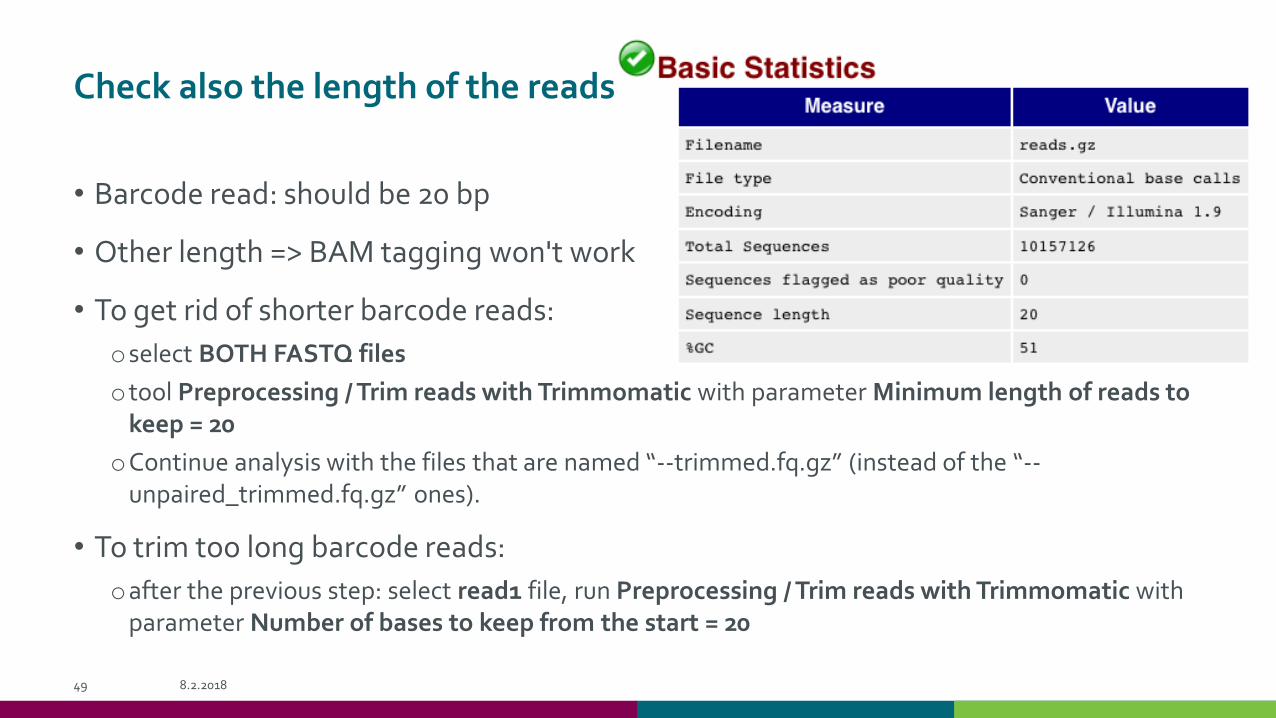
Check also the length of the reads
• Barcode read: should be 20 bp
• Other length => BAM tagging won't work
• To get rid of shorter barcode reads:
oselect BOTH FASTQ files
otool Preprocessing / Trim reads with Trimmomatic with parameter Minimum length of reads to keep = 20
oContinue analysis with the files that are named “--trimmed.fq.gz” (instead of the “--unpaired_trimmed.fq.gz” ones).
• To trim too long barcode reads:
oafter the previous step: select read1 file, run Preprocessing / Trim reads with Trimmomatic with parameter Number of bases to keep from the start = 20
8.2.201849

From FASTQ to expression matrix –preprocessing of DropSeq data
• Quality control of raw reads
• Preprocessing: tagging with barcodes & filtering
• Alignment to reference genome
• Merge BAM files
• Annotate with gene names
• Estimate the number of usable cells
• Detect bead synthesis errors
• Generate digital expression matrix
8.2.201850

Preprocessing single cell DropSeq FASTQ files
• This tool is a combination of several tools:
oDropSeq (TagBamWithReadSequenceExtended, FilterBam)
oPicard (FASTQ to BAM, BAM to FASTQ) and
o Trimmomatic (MINLEN)
• The steps are:
1. Convert the FASTQ files into an unaligned BAM file
2. Tag the reads in the BAM file with the cellular and molecular barcodes
3. Filter and trim the reads in the BAM file
4. Convert the tagged and trimmed BAM file back into a FASTQ file for the alignment
5. Filter out too short reads of the FASTQ file
8.2.201851
Why FASTQ-BAM-FASTQ-BAM?
-FASTQ format cannot hold the information about the cellular and molecular barcodes. BAM format has tag fields which can be used to hold this information
-In BAM format we can also do some trimming and filtering for the reads.
-However, the aligners take as input only FASTQ format, which is why we need to transform the trimmed & filtered BAM back to FASTQ format.
-Later on, after alignment, we merge the two!

Read1.fastq Read2.fastq
Unaligned_trimmed.bam
Import files
unaligned.fastq
Aligned.bam Aligner (STAR, HISAT)
Merged.bam Merge BAM
annotated.bamTag read with gene exon
Detect bead synthesis errorshistogram.pdf
digital_expression.tsv
BAM tag histogram
Digital expression
-filter bad qualitybarcodes
-trim adapter sequences
-trim polyA tails
Combines thebarcode tags and the alignment info
Pre
pro
cess
:
FASTQ to BAM
Tag BAM
Filter and trim BAM
BAM to FASTQ
Filter too short reads
FastQC.html FastQC.html
Quality control / FASTQC

Preprocessing single cell DropSeq FASTQ files, parameters
o Convert the FASTQ files into an unaligned BAM file
o Tag the reads in the BAM file with the cellular and molecular barcodes
o Filter and trim the reads in the BAM file
o Convert the tagged and trimmed BAM file back into a FASTQ file for the alignment
o Filter out too short reads of the FASTQ file
• Base range for cell barcode [1-12]
• Base range for molecule barcode [13-20]
• Base quality [10]
• Adapter sequence [AAGCAGTGGTATCAACGCAGAGTGAATGGG]
• Mismatches in adapter [0]
• Number of bases to check in adapter [5]
• Mismatches in polyA [0]
• Number of bases to check in polyA [6]
• Minimum length of reads to keep [50]8.2.201853

Preprocessing DropSeq FASTQ files –Tagging reads
• BAM tags
oXM = molecular barcode
oXC = cellular barcode
oXQ = number of bases that fall below quality threshold
• After this, we can forget the
barcode read
• You need to tell the tool which
bases correspond to which
barcode
8.2.201854

Preprocessing DropSeq FASTQ files –Trimming and filtering
• Quality: filter out reads where more
than 1 base have poor quality
• Adapters: Trim away any user
determined sequences
oSMART adapter as default
oHow many mismatches allowed (0)
oHow long stretch of the sequence there has to be at least (5 )
• polyA: hard-clip polyA tails
oHow many A’s need to be there before clipping happens (6 )
omismatches allowed (0)
• Minimum length: filter out short
reads from the FASTQ file55

From FASTQ to expression matrix –preprocessing of DropSeq data
• Quality control of raw reads
• Preprocessing: tagging with barcodes & filtering
• Alignment to reference genome
• Merge BAM files
• Annotate with gene names
• Estimate the number of usable cells
• Detect bead synthesis errors
• Generate digital expression matrix
8.2.201856

Alignment to reference genome
• Goal is to find out where a read originated fromoChallenge: variants, sequencing errors, repetitive sequence
• Many organisms have introns, so RNA-seq reads map to genome non-contiguously spliced alignments neededoBut sequence signals at splice sites are limited and introns can be thousands of bases long
• Splice-aware aligners
oHISAT2, TopHat
oSTAR

HISAT2
• HISAT = Hierarchical Indexing for Spliced Alignment of Transcripts
• Fast spliced aligner with low memory requirement
• Reference genome is indexed for fast searching
• Uses two types of indexes
oOne global index: used to anchor each alignment (28 bp is enough)
oThousands of small local indexes, each covering a genomic region of 56 Kbp: used for rapid extension of alignments (good for reads with short anchors over splice sites)
• Uses splice site information found during the alignment of earlier reads in
the same run
8.2.201858
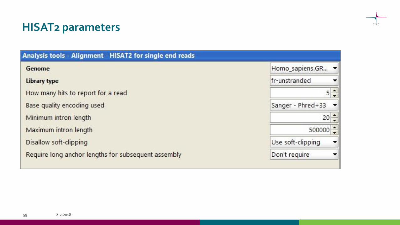
HISAT2 parameters
8.2.201859

STAR
STAR (Spliced Transcripts Alignment to a Reference) uses a 2-pass mapping process
• splice junctions found during the 1st pass are inserted into the genome index, and all reads are re-mapped in the 2nd mapping pass
• this doesn't increase the number of detected novel junctions, but it allows more spliced reads mapping to novel junctions.
Maximum alignments per read -parameter sets the maximum number of loci the read is allowed to map to
• Alignments (all of them) will be output only if the read maps to no more loci than this. Otherwise no alignments will be output.
Chipster offers an Ensembl GTF file to detect annotated splice junctions
• you can also give your own, for example GENCODE GTFs are recommended
Two log files
• Log_final.txt lists the percentage of uniquely mapped reads etc.
• Log_progress.txt contains process summary

• SAM (Sequence Alignment/Map) is a tab-delimited text file containing aligned reads. BAM is a binary (and hence more compact) form of SAM.
optional header section
alignment section: one line per read, containing 11 mandatory fields, followed by optional tags
BAM file format for aligned reads
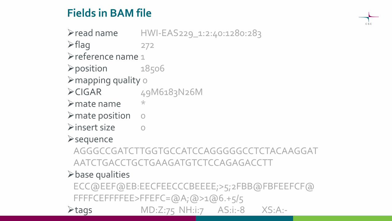
Fields in BAM file
read name HWI-EAS229_1:2:40:1280:283flag 272reference name 1position 18506mapping quality 0CIGAR 49M6183N26Mmate name *mate position 0insert size 0sequence
AGGGCCGATCTTGGTGCCATCCAGGGGGCCTCTACAAGGATAATCTGACCTGCTGAAGATGTCTCCAGAGACCTTbase qualities
ECC@EEF@EB:EECFEECCCBEEEE;>5;2FBB@FBFEEFCF@FFFFCEFFFFEE>FFEFC=@A;@>1@6.+5/5tags MD:Z:75 NH:i:7 AS:i:-8 XS:A:-

BAM index file (.bai)
• BAM files can be sorted by chromosomal coordinates and indexed for efficient
retrieval of reads for a given region.
• The index file must have a matching name. (e.g. reads.bam and reads.bam.bai)
• Genome browser requires both BAM and the index file.
• The alignment tools in Chipster automatically produce sorted and indexed BAMs.
• When you import BAM files, Chipster asks if you would like to preproces them
(convert SAM to BAM, sort and index BAM).
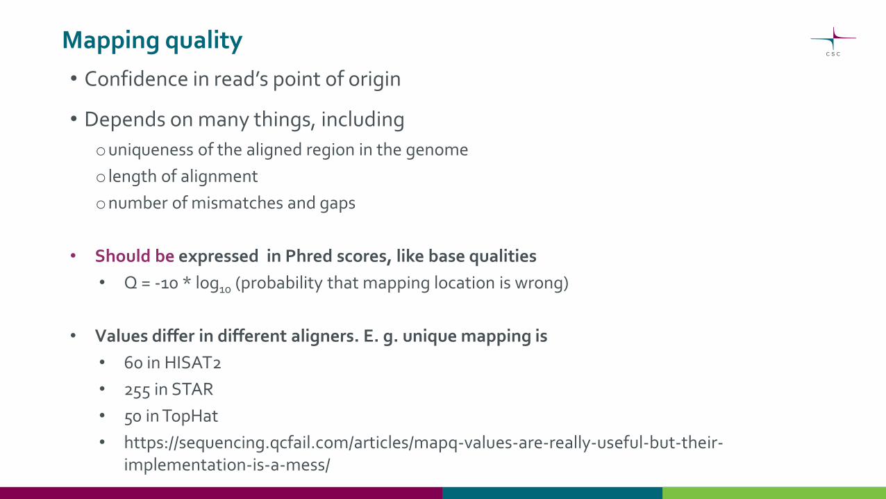
Mapping quality
• Confidence in read’s point of origin
• Depends on many things, including
ouniqueness of the aligned region in the genome
o length of alignment
onumber of mismatches and gaps
• Should be expressed in Phred scores, like base qualities
• Q = -10 * log10 (probability that mapping location is wrong)
• Values differ in different aligners. E. g. unique mapping is
• 60 in HISAT2
• 255 in STAR
• 50 in TopHat
• https://sequencing.qcfail.com/articles/mapq-values-are-really-useful-but-their-implementation-is-a-mess/

• Checks coverage uniformity, read distribution between different genomic
regions, novelty of splice junctions, etc.
• Takes a BAM file and a BED file
oChipster has BED files available for several organisms
oYou can also use your own BED if you prefer
Quality check after alignment with RseQC

Visualize alignments in genomic context: Chipster Genome Browser
• Integrated with Chipster analysis environment
• Automatic coverage calculation (total and strand-specific)
• Zoom in to nucleotide level
• Highlight variants
• Jump to locations using BED, GTF, VCF and tsv files
• View details of selected BED, GTF and VCF features
• Several views (reads, coverage profile, density graph)


From FASTQ to expression matrix –preprocessing of DropSeq data
• Quality control of raw reads
• Preprocessing: tagging with barcodes & filtering
• Alignment to reference genome
• Merge BAM files
• Annotate with gene names
• Estimate the number of usable cells
• Detect bead synthesis errors
• Generate digital expression matrix
8.2.201869

Read1.fastq Read2.fastq
Unaligned_trimmed.bam
Import files
unaligned.fastq
Aligned.bam Aligner (STAR, HISAT)
Merged.bam Merge BAM
annotated.bamTag read with gene exon
Detect bead synthesis errorshistogram.pdf
digital_expression.tsv
BAM tag histogram
Digital expression
-filter bad qualitybarcodes
-trim adapter sequences
-trim polyA tails
Combines thebarcode tags andthe alignment info
Pre
pro
cess
:
FASTQ to BAM
Tag BAM
Filter and trim BAM
BAM to FASTQ
Trim too short reads
FastQC.html FastQC.html
Quality control / FASTQC

Merge BAM files
• Why was this again…?
o In the alignment, we lost the molecular and cellular tag information (because aligners only eat FASTQ format). We have that info in the unaligned.BAM file, so now we combine the two.
• Before merging, the tool sorts the
files in queryname order
• Secondary alignments are ignored!
• Remember to…
oChoose the reference
oMake sure the files are correctly assigned!
8.2.201871

From FASTQ to expression matrix –preprocessing of DropSeq data
• Quality control of raw reads
• Preprocessing: tagging with barcodes & filtering
• Alignment to reference genome
• Merge BAM files
• Annotate with gene names
• Estimate the number of usable cells
• Detect bead synthesis errors
• Generate digital expression matrix
8.2.201872

Annotate
• GE-tag = name of the gene, if the read overlaps an exon
• XF-tag = location (intron, exon…)
• Choose the annotation file (GTF) OR use your own
8.2.201873

From FASTQ to expression matrix –preprocessing of DropSeq data
• Quality control of raw reads
• Preprocessing: tagging with barcodes & filtering
• Alignment to reference genome
• Merge BAM files
• Annotate with gene names
• Estimate the number of usable cells
• Detect bead synthesis errors
• Generate digital expression matrix
8.2.201874

Estimate the number of usable cells
• How many cells do you want to keep?
• To estimate this: the inflection point
1. extract the number of reads per cell (barcode)
2. plot the cumulative distribution of reads
3. select the “knee” of the distribution (knee = inflection point)
oThe number of STAMPs (=beads exposed to a cell in droplets): cell barcodes to the left of the inflection point
oEmpties (=beads only exposed to ambient RNA in droplets): to the right of the inflection point
8.2.201875
Inflection point
STAMPS
“empties”
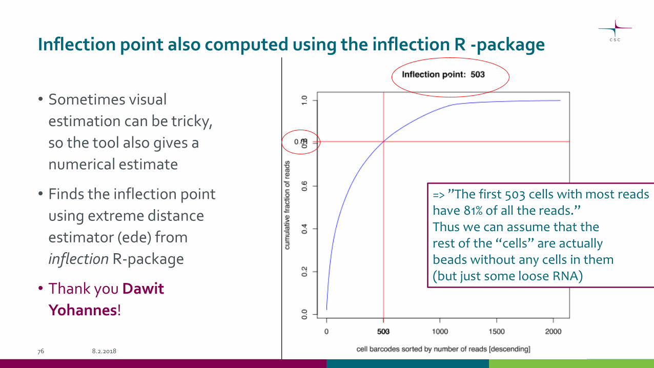
Inflection point also computed using the inflection R -package
• Sometimes visual
estimation can be tricky,
so the tool also gives a
numerical estimate
• Finds the inflection point
using extreme distance
estimator (ede) from
inflection R-package
• Thank you Dawit
Yohannes!
8.2.201876
=> ”The first 503 cells with most readshave 81% of all the reads.”Thus we can assume that the rest of the “cells” are actually beads without any cells in them (but just some loose RNA)
v
v

From FASTQ to expression matrix –preprocessing of DropSeq data
• Quality control of raw reads
• Preprocessing: tagging with barcodes & filtering
• Alignment to reference genome
• Merge BAM files
• Annotate with gene names
• Estimate the number of usable cells
• Detect bead synthesis errors
• Generate digital expression matrix
8.2.201877
Read1.fastq Read2.fastq
Unaligned_trimmed.bam
Import files
unaligned.fastq
Aligned.bam
Merged.bam Merge BAM
annotated.bamTag read with gene exon
Detect bead synthesis errorshistogram.pdf
digital_expression.tsv
BAM tag histogram
Digital expression
-filter bad qualitybarcodes
-trim adapter sequences
-trim polyA tails
To combine thebarcode tags and the alignment info
Pre
pro
cess
:
FASTQ to BAM
Tag BAM
Filter and trim BAM
BAM to FASTQ
Trim too short reads
FastQC.html FastQC.html
Quality control / FASTQC
Aligner (STAR, HISAT)
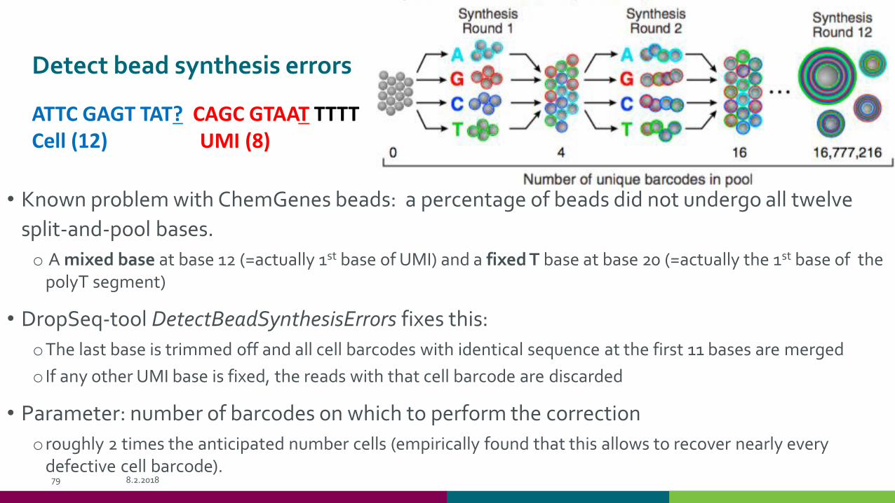
Detect bead synthesis errors
• Known problem with ChemGenes beads: a percentage of beads did not undergo all twelve
split-and-pool bases.
o A mixed base at base 12 (=actually 1st base of UMI) and a fixed T base at base 20 (=actually the 1st base of the polyT segment)
• DropSeq-tool DetectBeadSynthesisErrors fixes this:
oThe last base is trimmed off and all cell barcodes with identical sequence at the first 11 bases are merged
o If any other UMI base is fixed, the reads with that cell barcode are discarded
• Parameter: number of barcodes on which to perform the correction
oroughly 2 times the anticipated number cells (empirically found that this allows to recover nearly every defective cell barcode).
8.2.201879
ATTC GAGT TAT? CAGC GTAAT TTTTCell (12) UMI (8)

Error types
• SYNTHESIS_MISSING_BASE
o1 or more bases missing from cell barcode => T’s at the end of UMIs
oFix: insert an “N” (reading frame fixed) and merge. If more than 1 missing, discard these reads
• SINGLE_UMI_ERROR
oAt each position of the UMIs, single base appears in >80% of the UMIs for that cell.
oFix: cell barcodes with this property are dropped
• PRIMER_MATCH
oSame as with SINGLE_UMI_ERROR, + the UMI matches one of the PCR primers
oFix: these barcodes are dropped
• OTHER
oUMIs are extremely skewed towards at least one base, but not at all 8 positions
oFix: these barcodes are dropped
8.2.201880

Synthesis statistics
• synthesis_stats.txt contains a bunch of useful information:
1. CELL_BARCODE the 12 base cell barcode
2. NUM_UMI the number of total UMIs observed
3. FIRST_BIASED_BASE the first base position where any bias is observed (-1 for no detected bias)
4. SYNTH_MISSING_BASE as 3 but specific to runs of T’s at the end of the UMI
5. ERROR_TYPE
6. For bases 1-8 of the UMI, the observed base counts across all UMIs. This is a “|” delimited field, with counts of the A,C,G,T,N bases.
• synthesis_stats.summary.txt contains a histogram of the
SYNTHESIS_MISSING_BASE errors*, as well as the counts of all other errors,
the number of total barcodes evaluated, and the number of barcodes ignored. *1 or more bases missing from cell barcode => T’s at the end of UMIs
8.2.201881 A | C | G | T | N

From FASTQ to expression matrix –preprocessing of DropSeq data
• Quality control of raw reads
• Preprocessing: tagging with barcodes & filtering
• Alignment to reference genome
• Merge BAM files
• Annotate with gene names
• Estimate the number of usable cells
• Detect bead synthesis errors
• Generate digital expression matrix
8.2.201882

Digital expression matrix
• To digitally count gene transcripts:
1. a list of HQ UMIs in each gene, within each cell, is assembled
2. UMIs within edit distance = 1 are merged together
3. The total number of unique UMI sequences is counted
=> this number is reported as the number of transcripts of that gene for a given cell
8.2.201883

Filtering the data for DGE
• Why don’t we just take all the cells?
othe aligned BAM can contain hundreds of thousands of cell barcodes
oSome of them are “empties”
oSome cell (barcode)s contain just handful of reads
o It is painful to deal with a huge matrix.
• Filtering based on:
oNumber of core barcodes (top X cells with most reads)
oMinimum number of expressed genes per cell
8.2.201884
Inflection point
STAMPS
“empties”
NOTE: You can always also choose to have a bigger number of cells and use that for further analysis (Seurat has it’s own filtering tools)
NOTE: ”read” is a molecule here, which may or may not have the same/almost same UMI as another molecule

Filtering the data for DGE –huge number of reads
• What do you do if this happens?
oUse the “minimum number of expressed genes per cell” as a requirement
oDo you know how many cells to expect? Use that number!
oTake a large number of cells and filter in the Seurat tools
• Why this happens?
8.2.201885

Read1.fastq Read2.fastq
Unaligned_trimmed.bam
Import files
unaligned.fastq
Aligned.bam Aligner (STAR, HISAT)
Merged.bam Merge BAM
annotated.bamTag read with gene exon
Detect bead synthesis errorshistogram.pdf
digital_expression.tsv
BAM tag histogram
Digital expression
-filter bad qualitybarcodes
-trim adapter sequences
-trim polyA tails
Combines thebarcode tags andthe alignment info
Pre
pro
cess
:
FASTQ to BAM
Tag BAM
Filter and trim BAM
BAM to FASTQ
Trim too short reads
FastQC.html FastQC.html
Quality control / FASTQC
Clustering analysis with Seurat tools

Seurat http://satijalab.org/seurat
• Seurat combines dimensionality reduction and graph-based
partitioning algorithms for unsupervised clustering of single cells.
• The approach can be described briefly:
1. Identification of highly variable genes
2. Linear dimensionality reduction (PCA, principal component analysis) on variable genes
3. Determine significant principal components
4. Graph based clustering to classify distinct groups of cells
5. Non-linear dimensional reduction (t-SNE, t-Distributed Stochastic Neighbor Embedding) for cluster visualization
6. Marker gene discovery, visualization, and downstream analysis
8.2.201889

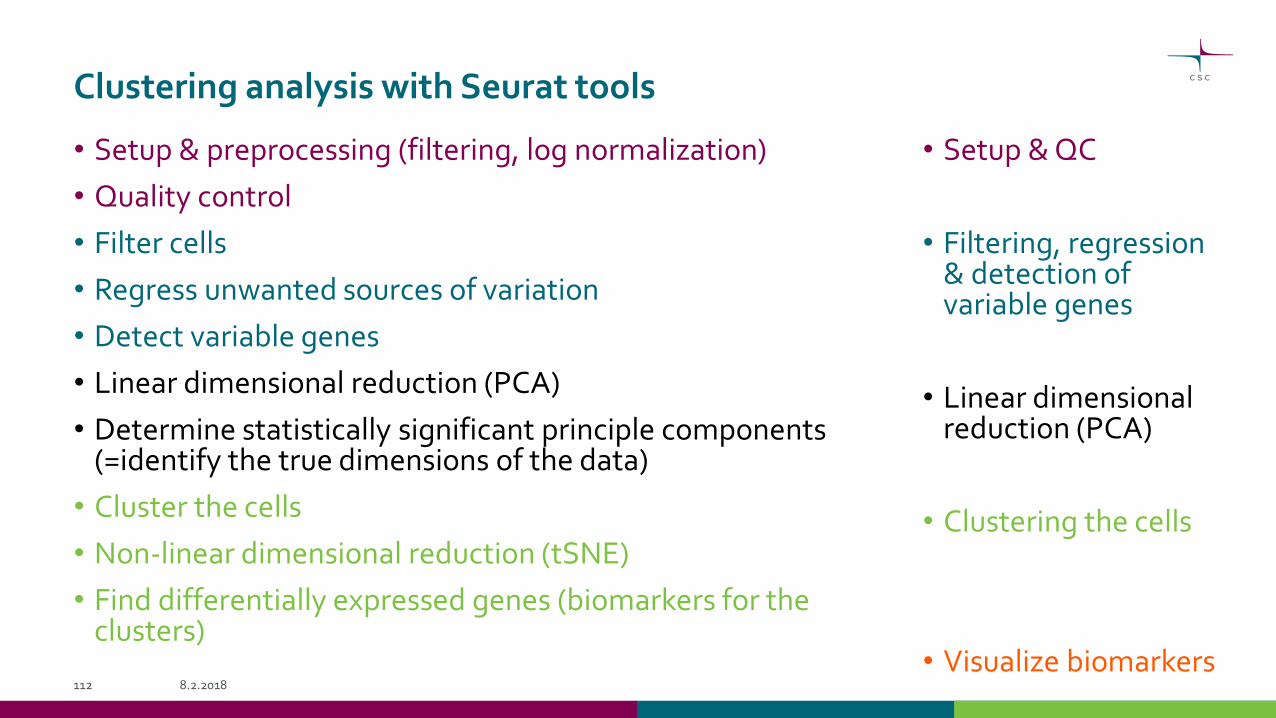
Clustering analysis with Seurat tools
• Setup & preprocessing (filtering, log normalization)
• Quality control
• Filter cells
• Regress unwanted sources of variation
• Detect variable genes
• Linear dimensional reduction (PCA)
• Determine statistically significant principle components (=identify the true dimensions of the data)
• Cluster the cells
• Non-linear dimensional reduction (tSNE)
• Find differentially expressed genes (biomarkers for the clusters)
8.2.201891
• Setup & QC
• Filtering, regression & detection of variable genes
• Linear dimensional reduction (PCA)
• Clustering the cells
• Visualize biomarkers

Setting up Seurat object
• In these tools, we are working with an R object (.Robj)
oCan’t be opened in Chipster, can be exported & imported to R
• Import one of the following
oTar package of three 10X Genomics output files
oDGE matrix from the DropSeq tools
oCheck that the input file is correctly assigned!
• Log normalization
onormalizes the gene expression measurements for each cell by the total expression, multiplies this by a scale factor (10,000 by default), and log transforms the result
• Filtering
oKeep genes which are detected at least in X cells
oKeep cells where at least Y genes are detected
• Give a name for the project (used in some plots)8.2.201892

Quality control & filtering for empties, multiplets and broken cells
• Empty (no cell in droplet)
low gene count (<200)
• Multiplet (more than one cell
in droplet) large gene
count (>2500)
• Broken cell in droplet
large percentage of
mitochondrial transcripts
(>5%)
8.2.201893

Clustering analysis with Seurat tools
• Setup & preprocessing (filtering, log normalization)
• Quality control
• Filter cells
• Regress unwanted sources of variation
• Detect variable genes
• Linear dimensional reduction (PCA)
• Determine statistically significant principle components (=identify the true dimensions of the data)
• Cluster the cells
• Non-linear dimensional reduction (tSNE)
• Find differentially expressed genes (biomarkers for the clusters)
8.2.201894
• Setup & QC
• Filtering, regression & detection of variable genes
• Linear dimensional reduction (PCA)
• Clustering the cells
• Visualize biomarkers

Remove unwanted sources of variation
• Single cell data typically contains 'uninteresting' variation
otechnical noise
obatch effects
ocell cycle stage, etc
• Removing this variation improves downstream analysis
• Seurat constructs linear models to predict gene expression based on user-defined
variables
obatch, cell alignment rate, no of detected molecules per cell, mitochondrial transcript percentage
oSeurat regresses the given variables individually against each gene, and the resulting residuals are scaled
oscaled z-scored residuals of these models are used for dimensionality reduction and clustering
oChipster currently uses the no of detected molecules per cell and mitochondrial transcript percentage
8.2.201895

Detection of variable genes
• Downstream analysis focuses on highly variable genes
• Seurat finds them in the following way
1. calculate the average expression and dispersion for each gene
2. place genes into bins based on expression
3. calculating a z-score for dispersion within each bin
• Set the parameters to mark visual outliers on the
dispersion plot
oexact parameter settings may vary based on the data type, heterogeneity in the sample, and normalization strategy
oThe default parameters are typical for UMI data that is normalized to a total of 10 000 molecules
8.2.201896

Clustering analysis with Seurat tools
• Setup & preprocessing (filtering, log normalization)
• Quality control
• Filter cells
• Regress unwanted sources of variation
• Detect variable genes
• Linear dimensional reduction (PCA)
• Determine statistically significant principle components (=identify the true dimensions of the data)
• Cluster the cells
• Non-linear dimensional reduction (tSNE)
• Find differentially expressed genes (biomarkers for the clusters)
8.2.201897
• Setup & QC
• Filtering, regression & detection of variable genes
• Linear dimensional reduction (PCA)
• Clustering the cells
• Visualize biomarkers

Linear dimensionality reduction (PCA) on variable genes
• Principal Component Analysis = PCA
• Reduce the numerous, possibly
correlating variables (=counts for
each gene) into a smaller number of
linearly uncorrelated dimensions
(=principal components)
• Essentially, each PC represents a
robust ‘metagene’ — a linear
combination of hundreds to
thousands of individual transcripts
8.2.201898
A dot = a cell

Determine significant principal components
• A key step to this clustering approach involves selecting a set of
principal components (PCs) for downstream clustering analysis
• However, estimating the true dimensionality of a dataset is a
challenging and common problem in machine learning.
• The tool provides a couple plots to aid in this:
oElbow plot
oPCHeatmap
8.2.201899

Determine significant principal components 1: Elbow plot
• The elbow in the plot tends to
reflect a transition from
informative PCs to those that
explain comparatively little
variance.
8.2.2018100
“How much variance each PC explains?”
Gaps?Plateau?

Determine significant principal components 2: PCHeatmap
• Displays the extremes across both
genes and cells, and can be useful
to help exclude PCs that may be
driven primarily by
ribosomal/mitochondrial or cell
cycle genes.
8.2.2018101
“Is there still a differencebetween the extremes?”

Clustering analysis of with Seurat tools
• Setup & preprocessing (filtering, log normalization)
• Quality control
• Filter cells
• Regress unwanted sources of variation
• Detect variable genes
• Linear dimensional reduction (PCA)
• Determine statistically significant principle components (=identify the true dimensions of the data)
• Cluster the cells
• Non-linear dimensional reduction (tSNE)
• Find differentially expressed genes (biomarkers for the clusters)
8.2.2018103
• Setup & QC
• Filtering, regression & detection of variable genes
• Linear dimensional reduction (PCA)
• Clustering the cells
• Visualize biomarkers

Clustering -why is it so tricky?
• Need to use unsupervised methods (we don’t
know beforehand, how many clusters there are)
• Our data is big and complex:
oLots of cells
oLots of dimensions (=genes)
oLots of noise (both technical and biological)
• …which is why:
o the algorithm is a bit tricky, and
oWe reduce and select the dimensions to use in clustering (= we do the PCA and select X components to use, instead of using all thoudans of genes)
8.2.2018105
KNN in 2D with know clusters –this would be nice and easy!

• Seurat clustering = similar to
oSNN-Cliq (C. Xu and Su, Bioinformatics 2015) and
oPhenoGraph (Levine et al. Cell 2015)
• ...which are graph based methods:
1. Identify k-nearest neighbours of each cell
oDistance measure: Euclidean + Jaccard distance
2. Calculate the number of Shared Nearest Neighbours (SNN) between each pair of cells
3. Build the graph: add an edge between cells, if they have at least one SNN
4. Clusters: group of cells with many edges between them
o Smart Local Moving algorithm (SLM, Blondel et al., Journal of Statistical Mechanics)
8.2.2018106
Graph based clustering to classify distinct groups of cells
KNN:
Graph:
cell
edge
cell

Clustering parameters
• Lots of parameters!
• Dims.use = number of principal components
• Resolution = “granularity”:
o increased values lead to a greater number of clusters.
oValues 0.6-1.2 typically returns good results for single cell datasets of around 3K cells
oOptimal resolution often increases for larger datasets
o (If you get very few or very many clusters, try adjusting)
8.2.2018107
FindClusters(object, genes.use = NULL, reduction.type = "pca", dims.use = NULL, k.param = 30, k.scale = 25, plot.SNN = FALSE, prune.SNN = 1/15, print.output = TRUE, distance.matrix = NULL, save.SNN = FALSE, reuse.SNN = FALSE, force.recalc = FALSE, modularity.fxn = 1, resolution = 0.8, algorithm = 1, n.start = 100, n.iter = 10, random.seed = 0, temp.file.location = NULL)

Non-linear dimensional reduction (t-SNE) for cluster visualization
8.2.2018108
• T-SNE = t-distributed Stochastic Neighbor
Embedding
oNon-linear algorithm, different transformations to different regions
• Why do we now use t-SNE, why not the good
old PCA?
oWe give the selected PCA “pseudo-genes” to t-SNE
oT-SNE also reduces dimensions, but it is “more faithful to the original data”
oPCA can find clusters too, but t-SNE does just that –it reduced the dimensions so that the clusters become visible
• Good text about readingT-SNE’s:
https://distill.pub/2016/misread-tsne/
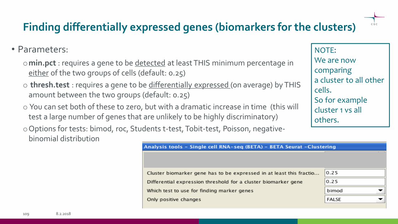
Finding differentially expressed genes (biomarkers for the clusters)
• Parameters:
omin.pct : requires a gene to be detected at least THIS minimum percentage in either of the two groups of cells (default: 0.25)
o thresh.test : requires a gene to be differentially expressed (on average) by THIS amount between the two groups (default: 0.25)
o You can set both of these to zero, but with a dramatic increase in time (this will test a large number of genes that are unlikely to be highly discriminatory)
oOptions for tests: bimod, roc, Students t-test, Tobit-test, Poisson, negative-binomial distribution
8.2.2018109
NOTE:We are now comparinga cluster to all other cells.So for example cluster 1 vs all others.

Markers for a particular cluster
• You can filter the resulting list to get only the biomarkers for a
certain cluster:
8.2.2018110

Visualize biomarkers
• Select a marker gene
from the lists
8.2.2018111
Clustering analysis with Seurat tools
• Setup & preprocessing (filtering, log normalization)
• Quality control
• Filter cells
• Regress unwanted sources of variation
• Detect variable genes
• Linear dimensional reduction (PCA)
• Determine statistically significant principle components (=identify the true dimensions of the data)
• Cluster the cells
• Non-linear dimensional reduction (tSNE)
• Find differentially expressed genes (biomarkers for the clusters)
8.2.2018112
• Setup & QC
• Filtering, regression & detection of variable genes
• Linear dimensional reduction (PCA)
• Clustering the cells
• Visualize biomarkers