Single-Element Characterization of the LS-DYNA MAT54 Material Model

Morgan Osborne

A thesis

submitted in partial fulfillment of the

requirements for the degree of

Master of Science

University of Washington

2012

Committee:

Paolo Feraboli

Uri Shumlak

Program Authorized to Offer Degree:

Aeronautics & Astronautics

Abstract Research was completed to characterize the root behavior of the LS-DYNA MAT54 composite orthotropic material model. This primarily involved investigating the constitutive relations, ply failure (damage onset), ply deletion, damage factors, and element deletion. A single shell element under uniaxial tensile and compressive loading was employed to isolate MAT54 behavior for three different idealized laminates. Simulation results were compared against expected behavior from published material properties and experimental testing. A parametric study was also conducted to confirm the behavior of all other MAT54 inputs. Overall the LS-DYNA MAT54 material model adequately predicted Unidirectional (UD), cross-ply, and fabric laminate behavior for the majority of cases. However, results showed pronounced plasticity when the strength-based Chang-Chang ply-failure criteria was reached prior to the strain-based ply-deletion parameters. This led to significant energy and failure strain errors in some cases.

i

Table of Contents

List of Figures ............................................................................................................................................... iii

List of Tables ................................................................................................................................................. v

Acknowledgements ...................................................................................................................................... vi

1. Introduction .......................................................................................................................................... 1

1.1 Methodology ................................................................................................................................. 3

1.2 Scope ............................................................................................................................................. 4

1.3 Selected Laminates ....................................................................................................................... 5

2. Experimental Baselines ......................................................................................................................... 6

2.1 Published Material Properties ...................................................................................................... 7

2.2 Expected Responses ...................................................................................................................... 8

2.2.1 UD.......................................................................................................................................... 8

2.2.2 Cross-Ply ................................................................................................................................ 8

2.2.3 Fabric ................................................................................................................................... 10

2.3 Experimental Setup ..................................................................................................................... 11

2.4 Experimental Results .................................................................................................................. 13

2.4.1 UD........................................................................................................................................ 13

2.4.2 Cross-Ply .............................................................................................................................. 15

2.4.3 Fabric ................................................................................................................................... 19

3. Numerical Simulations ........................................................................................................................ 24

3.1 LS-DYNA MAT54 Material Model ................................................................................................ 24

3.1.1 Overview ............................................................................................................................. 24

3.1.2 Constitutive ......................................................................................................................... 24

3.1.3 Ply Failure (Damage Onset) ................................................................................................. 25

3.1.4 Damage Factors .................................................................................................................. 27

3.1.5 Ply Deletion ......................................................................................................................... 28

3.1.6 Element Deletion ................................................................................................................ 28

3.2 LS-DYNA Single Element Simulation Setup ................................................................................. 29

3.2.1 Common Setup ................................................................................................................... 29

3.2.2 UD Setup ............................................................................................................................. 31

3.2.3 Cross-Ply Setup .................................................................................................................... 33

ii

3.2.4 Fabric Setup ........................................................................................................................ 35

3.3 Results ......................................................................................................................................... 36

3.3.1 UD Results ........................................................................................................................... 36

3.3.2 Cross-Ply Results ................................................................................................................. 55

3.3.3 Fabric Results ...................................................................................................................... 75

4. Research Summary and Conclusions .................................................................................................. 91

5. Bibliography ........................................................................................................................................ 93

Appendix A. MAT54 Input Parameter Definitions ................................................................................... 95

Appendix B. Baseline LS-DYNA Input Decks ............................................................................................ 97

B1. UD [0]12 Tension .......................................................................................................................... 97

B2. Cross-Ply [0/90]3S Tension ......................................................................................................... 100

B3. Fabric [0f]8 Tension .................................................................................................................... 103

iii

List of Figures Figure 1. Research Scope ............................................................................................................................. 4 Figure 2. Cross-Ply Springs-in-Parallel Analog .............................................................................................. 8 Figure 3. Representative Test Setup .......................................................................................................... 11 Figure 4. Baseline UD Stress vs. Strain – All Specimens ............................................................................. 13 Figure 5. Baseline Cross-Ply Stress vs. Strain – Strain Gage Specimens Only ............................................ 16 Figure 6. Baseline Cross-Ply Stress vs. Strain – All Specimens ................................................................... 17 Figure 7. Baseline Cross-Ply Energy vs. Strain – All Specimens .................................................................. 17 Figure 8. Baseline Cross-Ply Load vs. Displacement – All Specimens ........................................................ 18 Figure 9. Baseline [0f]8 Fabric Stress vs. Strain – All Specimens ................................................................. 20 Figure 10. Baseline [0f]8 Fabric Energy vs. Strain – All Specimens ............................................................. 21 Figure 11. Baseline [0f]8 Fabric Load vs. Displacement – All Specimens .................................................... 22 Figure 12. Baseline Fabric and Cross-Ply Stress vs. Strain – All Specimens ............................................... 23 Figure 13. MAT54 Input Card ..................................................................................................................... 24 Figure 14. Typical Ply Stress-Strain Behavior ............................................................................................. 26 Figure 15. Single Element Mesh, Boundary Conditions, & Loading ........................................................... 29 Figure 16. LS-DYNA Cross-Ply Simulations – Loading and Boundary Conditions ....................................... 33 Figure 17. Mapping of Fabric Properties to MAT54 Material System ....................................................... 35 Figure 18. Baseline UD [0]12 Stress vs. Strain – Expected & LS-DYNA MAT54 ........................................... 36 Figure 19. Baseline UD [0]12 Energy vs. Strain – Expected & LS-DYNA MAT54 .......................................... 37 Figure 20. Baseline UD [90]12 Stress vs. Strain – Expected & LS-DYNA MAT54 ......................................... 37 Figure 21. Baseline UD [90]12 Energy vs. Strain – Expected & LS-DYNA MAT54 ........................................ 38 Figure 22. UD [0]12 Parametric Study – Longitudinal/Fiber Modulus (EA) Stress vs. Strain ...................... 40 Figure 23. UD [0]12 Parametric Study – Longitudinal Strength – Stress vs. Strain ..................................... 41 Figure 24. UD [0]12 Parametric Study – Reduced Ply Strengths – Stress and Energy vs. Strain ................. 42 Figure 25. UD [0]12 Parametric Study – Longitudinal Failure Strains – Stress vs. Strain ............................ 43 Figure 26. UD [0]12 Parametric Study – Large Longitudinal Failure Strains – Stress vs. Strain .................. 44 Figure 27. UD [0]12 Parametric Study – DFAILT = 0 – Stress vs. Strain ....................................................... 45 Figure 28. UD [0]12 Parametric Study – EFS – Stress vs. Strain .................................................................. 46 Figure 29. UD [0]12 Parametric Study – Time Step Criteria TFAIL – Stress vs. Strain ................................. 47 Figure 30. UD [90]12 Parametric Study – Transverse/Matrix Modulus (EB) Stress vs. Strain .................... 48 Figure 31. UD [90]12 Parametric Study – Transverse Tensile Strength (YT) Stress vs. Strain ..................... 49 Figure 32. UD [90]12 Parametric Study – Transverse Compressive Strength (YC) Stress vs. Strain ........... 49 Figure 33. UD [90]12 Parametric Study – Transverse Failure Strain (DFAILM) Stress vs. Strain ................. 50 Figure 34. UD [90]12 Parametric Study – Transverse Failure Strain (DFAILM) Stress vs. Strain ................. 51 Figure 35. Ply Stress-Strain Behavior as Function of DFAIL Failure Strain ................................................. 53 Figure 36. Baseline Cross-Ply Stress vs. Strain – Test, Expected, & LS-DYNA MAT54 ................................ 55 Figure 37. MAT54 Fiber/1-Dir, Matrix/2-Dir, & Average Behavior ............................................................ 56 Figure 38. Baseline Cross-Ply Energy vs. Strain – Test, Expected, & LS-DYNA MAT54 .............................. 57 Figure 39. Baseline Cross-Ply Load vs. Displacement – Test, Expected, & LS-DYNA MAT54 ..................... 57 Figure 40. Baseline Cross-Ply Plots – Laminate and Ply Stresses ............................................................... 59

iv

Figure 41. Baseline Cross-Ply Plots – Ply Stresses and History Variables ................................................... 60 Figure 42. Cross-Ply Parametric Study – Fiber/1-Dir Modulus (EA) Plots .................................................. 61 Figure 43. Cross-Ply Parametric Study – Matrix/2-Dir Modulus (EB) Plots ................................................ 62 Figure 44. Cross-Ply Parametric Study – Fiber Tensile Strength (XT) Plots – Tensile Loading ................... 63 Figure 45. Cross-Ply Parametric Study – Fiber Tensile Strength (XT) Plots – Compressive Loading .......... 64 Figure 46. Cross-Ply Parametric Study – Fiber Compressive Strength (XC) Plots ...................................... 65 Figure 47. Cross-Ply Parametric Study – Matrix Tensile Strength (YT) Plots ............................................. 66 Figure 48. Cross-Ply Parametric Study – Matrix Compressive Strength (YC) Plots .................................... 67 Figure 49. Cross-Ply Parametric Study – Fiber Tensile Strain (DFAILT) Plots ............................................. 68 Figure 50. Cross-Ply Parametric Study – Fiber Compressive Strain (DFAILC) Plots .................................... 69 Figure 51. Cross-Ply Parametric Study – Matrix Strain (DFAILM) Plots ..................................................... 70 Figure 52. Cross-Ply Parametric Study – Matrix Strain (DFAILM) Plots & Theoretical Response .............. 71 Figure 53. Comparison of Theoretical (AGATE-Based) and LS-DYNA Fiber Stress vs. Strain ..................... 73 Figure 54. Baseline [0f]8 Fabric Stress vs. Strain – Expected & LS-DYNA MAT54 ....................................... 75 Figure 55. Baseline [0f]8 Fabric Stress vs. Strain – LS-DYNA MAT54 Plasticity ........................................... 76 Figure 56. Baseline [0f]8 Fabric Energy vs. Strain – Expected & LS-DYNA MAT54...................................... 77 Figure 57. Baseline [0f]8 Fabric History Variable vs. Strain – LS-DYNA MAT54 .......................................... 78 Figure 58. Baseline [90f]8 Fabric Stress vs. Strain – Expected & LS-DYNA MAT54 ..................................... 79 Figure 59. Baseline [90f]8 Fabric Energy vs. Strain – LS-DYNA MAT54 ....................................................... 80 Figure 60. Stress vs. Strain – Comparison of Baseline Fabric and Cross-Ply .............................................. 82 Figure 61. [0f]8 Fabric Parametric Study – Long. Modulus (EA) Plots ........................................................ 83 Figure 62. [90f]8 Fabric Parametric Study – Tran. Modulus (EB) Plots ....................................................... 84 Figure 63. [0f]8 Fabric Parametric Study – Long. Tensile Strength (XT) Plots ............................................. 85 Figure 64. [0f]8 Fabric Parametric Study – Long. Compressive Strength (XC) Plots ................................... 86 Figure 65. [0f]8 Fabric Parametric Study – Long. Tensile Failure Strain (DFAILT) Plots .............................. 87 Figure 66. [0f]8 Fabric Parametric Study – Long. Compressive Failure Strain (DFAILC) Plots ..................... 87 Figure 67. [90f]8 Fabric Parametric Study – Transverse Failure Strain (DFAILM) Plots .............................. 88 Figure 68. Comparison of Expected and MAT54 Transverse Behavior ...................................................... 88 Figure 69. [90f]8 Fabric Parametric Study – Transverse Failure Strain (DFAILM) Plots .............................. 89

v

List of Tables Table 1. Comparison of Result Quantities.................................................................................................... 6 Table 2. Toray T700GC-12K-31E/#2510 UD Tape Properties ....................................................................... 7 Table 3. Toray T700SC-12K-50C/#2510 Plain-Weave Fabric Properties ...................................................... 7 Table 4. UD Experimental Test Matrix ....................................................................................................... 12 Table 5. Cross-Ply Experimental Test Matrix ............................................................................................. 12 Table 6. Fabric Experimental Test Matrix .................................................................................................. 12 Table 7. [0]12 UD Baseline Results – Experimental & Theory ..................................................................... 13 Table 8. [90]12 UD Baseline Results – Experimental & Theory ................................................................... 14 Table 9. Cross-Ply Baseline Results – Experimental & Theory ................................................................... 15 Table 10. [0f]8 Fabric Baseline Results – Experimental & Expected ........................................................... 19 Table 11. Fabric Longitudinal (1-dir) and Transverse (2-dir) Expected Properties .................................... 20 Table 12. UD [0]12 Parametric Study – Simulation Matrix ......................................................................... 31 Table 13. UD [90]12 Parametric Study – Simulation Matrix........................................................................ 32 Table 14. Cross-Ply Parametric Study – Simulation Matrix ........................................................................ 34 Table 15. Fabric Parametric Study – Simulation Matrix ............................................................................. 35 Table 16. UD [0]12 Baseline Results – Expected & LS-DYNA MAT54 .......................................................... 39 Table 17. UD [90]12 Baseline Results – Expected & LS-DYNA MAT54 ........................................................ 39 Table 18. [90]12 Parametric Study – Matrix Strain (DFAILM) Error Summary ............................................ 52 Table 19. Cross-Ply Baseline Results – LS-DYNA MAT54 & Theory ............................................................ 58 Table 20. Cross-Ply Parametric Study – Matrix Strain (DFAILM) Error Summary ...................................... 72 Table 21. Baseline [0f]8 LS-DYNA MAT54 Error ........................................................................................... 81 Table 22. Baseline [90f]8 LS-DYNA MAT54 Error ........................................................................................ 81 Table 23. Fabric Parametric Study – Transverse Strain (DFAILM) Error Summary .................................... 89

vi

Acknowledgements The author would like to thank Bonnie Wade for penning the first iteration of the introduction and unidirectional sections. Further, her patience in answering my many questions was greatly appreciated. I’d also like to thank Professor Paolo Feraboli for his overall guidance through the research process and Professor Uri Shumlak for his inputs. Finally, this thesis could not have been completed without the support, understanding, and patience of my family and friends.

1

1. Introduction The numeric simulation of laminated composites beyond the elastic region in a crash simulation is a great challenge due to the complex combination of failure mechanisms that occur within the laminate. These include fiber fracture, matrix cracking, and inter-laminar damage, all of which can occur alone or in combination. In addition, the overall response of the composite structure is highly dependent on several parameters including geometry, material system, lay-up, and impact velocity [1][2].

It is well accepted in the composites community that existing failure criteria for composites have several shortcomings, making it a challenge to predict even the onset of damage [3][4]. The critical need for a predictive material model has driven international research efforts and produced an abundance of literature on dynamic simulations of composite structures in the last two decades [3][4][5][6][7][8].

The state-of-the-art finite element (FE) codes used to predict the dynamic damage of composite and metallic materials alike, such as LS-DYNA, ABAQUS Explicit, RADIOSS, and PAM-CRASH, implement internally-developed composite material models to define the elastic, failure, and post-failure behavior of the elements. These material models account for physical properties of the material that can be measured by experiment (such as strength, modulus, and strain-to-failure) but also include software-specific parameters, which either have no physical meaning or cannot be determined experimentally. Usage of non-physical parameters thus requires extensive calibration and tweaking of these material models in order to reach an agreement between experiment and simulation.

The FE codes utilize an explicit integration formulation that is computationally very expensive. As a consequence, shell (2D) elements are preferred over the more costly brick (3D) elements and composites are typically modeled as orthotropic shell elements with smeared material properties. The plies of the laminate are grouped into a single shell element, which reduces the level of computational effort but does not capture inter-laminar behavior. Current FE modeling strategies for composite materials are therefore not deemed to be predictive as demonstrated by efforts such as the Worldwide Failure Exercise [3] and the CMH-17 crashworthiness numerical round robin [4].

Although several other codes are available, LS-DYNA has traditionally been considered the benchmark for composite crash simulations and is extensively used in the automotive and aerospace industries to perform explicit dynamic post-failure simulations [9][10][11]. LS-DYNA has a handful of preexisting composite material models such as MAT22, MAT54, and MAT55, which are progressive failure models that use a ply discount method to degrade elastic material properties. MAT58, MAT158, and MAT162 are also available, which use continuum damage mechanics to degrade the elastic properties after failure.

2

The LS-DYNA MAT54 material model is of interest for large full-scale structural damage simulations because it is a relatively simple material model with minimal input parameters. Not only does this reduce the computational requirement of a simulation, it also reduces the difficulty and amount of material testing necessary to generate the input parameters.

The relative simplicity of MAT54, however, can create notable shortcomings as a consequence of over-simplifying the complex physical mechanics occurring during composite failure. For example, the MAT54 model exhibited unanticipated plasticity in composite crash simulations developed at the University of Washington; this plasticity was also seemingly inconsistent with LS-DYNA documentation.

Therefore, research was completed to characterize the LS-DYNA MAT54 material model and identify any shortcomings. The research included a review of the MAT54 documentation and a set of single element LS-DYNA simulations for three laminates amongst two carbon fiber/epoxy material systems. The research methodology is provided in the following section.

3

1.1 Methodology Prior to performing the LS-DYNA MAT54 single element simulations, LS-DYNA documentation [12] for the MAT54 material model was reviewed. The purpose was to catalog the key input parameters and understand the constitutive, ply-failure, and ply-deletion models. The review incorporated knowledge gained from this research and is provided to familiarize the reader with the material model.

After completing the LS-DYNA MAT54 material model review, an appropriate carbon fiber/epoxy material system and idealized laminates (lay-ups) were chosen for the simulations. Published material properties for Unidirectional (UD) tape and plain-weave fabric were obtained and were used to define baselines for simulation comparisons (i.e. they represented the expected simulation behavior).

Experimental testing of the same laminates was also completed to confirm the expected behavior and fill-in any missing information (for example, full-range stress versus strain curves). Experimental tests included uniaxial tension and compression specimens about the two material axes. Published data, experimental results, and applicable hand calculations are provided in the experimental section.

Next LS-DYNA single-element simulations were completed for the UD, cross-ply, and fabric laminates and compared against the expected baselines. The baseline simulations helped characterize the MAT54 material model for idealized laminates under simplified loading. The simulation results and LS-DYNA setup are provided in the numerical simulation section.

Parametric studies of MAT54 material model inputs were also completed for each of the three laminates to further explore the MAT54 stress-strain envelope and identify any trends that were not witnessed in the baseline simulations. Another goal of the studies was to determine if the baseline MAT54 parameters were optimally chosen to minimize simulation error.

4

1.2 Scope The purpose of this research was to understand the elementary behavior of the MAT54 material model. Simulations were thus limited to a single LS-DYNA shell element under uniaxial tension and compression; shear, bending, and mixed loading conditions were considered beyond the scope of this research due to the complexity of failure modes, testing, and post-processing. Restricting the mesh to a single element allowed all element/material outputs to be reviewed, including integration point history variables that reported ply- and element-failure. Using a single element also eliminated any complications with stress concentrations, mesh sensitivity, etc.

Figure 1. Research Scope

As shown in Figure 1, restricting the scope to a single element under uniaxial tension/compression yielded two intended outcomes; first, material inputs only depended on experimentally derived quantities (for example, material strengths, moduli, and failure strains). Second, simulation results had the potential to be predictive as the MAT54 non-physical parameters (e.g. crush-specific factors, fiber damage factors, shear weighting factors) were expected to be inactive.

5

1.3 Selected Laminates Three different laminates based on carbon-epoxy material systems were explored in the research. The first was a [0]12 lay-up of UD tape. This laminate simplified the task of exploring the underlying MAT54 material behavior as laminate- and ply-stresses were identical. Laminate behavior about the longitudinal and transverse material axes were explored with [0]12 and [90]12 lay-ups respectively.

The second laminate was a [0/90]3S cross-ply lay-up of the same UD tape. Unlike single orientation layups, laminate stiffness was dependent on the lay-up and both progressive ply failure and off-axis stresses were present. Cross-ply layups offered a manageable increase in complexity and were desired for being more representative of an actual quasi-isotropic layup. They also presented an opportunity to verify if the laminate response could be predicted solely based on lamina properties and a known lay-up. Cross-ply laminates were also desired for eliminating any internal ply coupling between axial, bending, and shear (per Classical Lamination Theory (CLT)) under axial loading.

The last laminate used the same carbon fiber and matrix constituents as the UD tape except in fabric form. The [0f]8 fabric lay-up was loaded about both material axes and was desired for drawing a comparison between UD tape and fabric responses.

6

2. Experimental Baselines The purpose of this section was to develop experimental baselines for later comparison with LS-DYNA MAT54 numerical simulations of the UD [0]12, cross-ply [0/90]3S, and fabric [0f]8 laminates. “Actual” and “expected” experimental baselines were established from experimental test data and published material properties respectively. The former was the benchmark of real-world behavior but did come with a disadvantage; namely the scatter associated with small sample sizes that made comparisons difficult. Comparing experimental and simulated results also internalized two sources of error: experimental (testing, manufacturing, etc.) and numerical (deviations from theory/expected).

In contrast the expected results, calculated from published material properties and actual specimen geometry, eliminated the experimental scatter and represented the anticipated response of a large sample size. Simulation errors were ultimately considered against these “expected” baselines.

The following laminate-level or macroscopic results were compared: elastic moduli, tensile and compressive strengths, full-range stress vs. strain curves, load vs. displacement curves, and finally overall energy. Table 1 highlights the relative worth of the various laminate results.

Table 1. Comparison of Result Quantities

Property Pros Cons Failure Load Tight experimental grouping;

accurate/direct measurement Geometry-dependent (i.e. not a material property)

Modulus Characterizes laminate stiffness; easy to measure

Requires accurate strain readings

Laminate Strength

Fundamental property

Stress vs. Strain Curve

Captures full laminate response (linear/non-linear, brittle/ductile, etc.)

Requires accurate strain readings; destroys strain gages

Failure Strain

Key parameter in numerical simulations Requires accurate strain readings; destroys strain gages

Energy Useful output in crash simulations Compounds error due to integration

7

2.1 Published Material Properties The first composite material system used for this study was Toray T700GC-12K-31E/#2510 Unidirectional Tape. This material system was well documented as part of the FAA-sponsored Advanced General Aviation Transport Experiments (AGATE) Program [13]; the system was also documented in the Composites Material Handbook (MIL-HDBK-17 / CMH-17) [4]. Strength and moduli from both references are shown in Table 2 along with values used in the LS-DYNA simulations. Also included in the table (but not part of the published data) are estimated failure strains assuming brittle failure.

Table 2. Toray T700GC-12K-31E/#2510 UD Tape Properties

The second material system used was Toray T700SC-12K-50C/#2510 plain-weave fabric, which was also documented for the AGATE [14] Program and CMH-17 [4]. Table 3 lists strengths, moduli, and estimated failure strains for both references along with those in the LS-DYNA simulations.

Table 3. Toray T700SC-12K-50C/#2510 Plain-Weave Fabric Properties

It should be noted that the fiber and matrix constituents for the UD and fabric systems were the same. The LS-DYNA MAT54 values were derived from previous research conducted at the University of Washington and some differed from published due to restrictions in the MAT54 material model (e.g. single modulus for both tension and compression).

Matl. Dir. Property Units AGATE

MIL-HDBK-17 DYNA AGATE

MIL-HDBK-17 DYNA

Strength ksi 314 319 319 210 213 213Modulus Msi 18.1 18.4 18.4 16.3 16.5 18.4

Strain u in/in 17,366 17,337 17,400 12,846 12,909 11,600Strength ksi 7.09 7.09 7.09 28.8 28.8 28.8Modulus Msi 1.22 1.22 1.22 1.22 1.47 1.22

Strain u in/in 5,813 5,811 24,000 23,618 19,592 24,000

Tension Compression

1/Fiber

2/ Matrix

Matl. Dir. Property Units AGATE

MIL-HDBK-17 DYNA AGATE

MIL-HDBK-17 DYNA

Strength ksi 133 133 132 103 103 103Modulus Msi 8.16 8.05 8.11 8.09 7.99 8.11

Strain u in/in 16,306 16,522 16,400 12,717 12,891 13,000Strength ksi 112 112 112 102 102 102Modulus Msi 7.96 7.94 7.89 7.77 7.76 7.89

Strain u in/in 14,132 14,106 14,000 13,127 13,144 14,000

Tension Compression

1/Long.

2/Tran.

8

2.2 Expected Responses

2.2.1 UD Expected UD responses used the AGATE data from Table 2. Recognizing laminate- and ply-responses were identical for the single-orientation ply lay-up, the AGATE data represented the expected response.

However, the AGATE design allowables report for this UD material system did not include strain to failure values [13]. Instead, the report suggested using a simple linear stress-strain relationship to obtain corresponding failure strain values. While this would be a valid assumption for fiber-dominated laminates, matrix-dominated laminates (such as [90]12) exhibit a non-linear response. Regardless, failure strains were calculated per Equation (1) by dividing the material strength (Fu) by the appropriate modulus (E).

𝜀fail =𝐹u

𝐸 (1)

Finally, average specimen geometry from the University of Washington test data were used to calculate peak loads (P) and energy (U) per Equations (2) and (3) respectively.

𝑃 = 𝐹u ∙ 𝐴lam (2)

𝑈 = 12𝐸lam𝐴lam𝐿lam(𝜀fail)2 (3)

2.2.2 Cross-Ply The simple cross-ply lay-up allowed laminate response to be calculated solely with Strength of Materials calculations (i.e. CLT was not required) by treating the equal-area groupings of 0º and 90º plies as two springs in parallel. Relevant formulas ((4) through (7)) are provided following Figure 2. Note that the “0” and “90” subscripts refer to the associated ply groups, while “t” denotes tension.

Figure 2. Cross-Ply Springs-in-Parallel Analog

k0º

P

[0/90]3S

P

k90º

9

𝐸𝑡,lam =𝐸1𝑡𝐴0 + 𝐸2𝑡𝐴90

𝐴0 + 𝐴90=𝐸1𝑡 + 𝐸2𝑡

2 (4)

𝑘t,lam =𝐸𝑡,lam𝐴lam

𝐿lam (5)

𝑃 = ∆𝐿 ∙ 𝑘t,lam =∆𝐿 ∙ 𝐸𝑡,lam ∙ 𝐴lam

𝐿lam (6)

𝑈 = energy = �𝑃(𝑥)𝑑𝑥 = 12𝑘t,lam𝑥2 ≈�

𝑃𝑖+1 + 𝑃𝑖2

(𝑥𝑖+1 − 𝑥𝑖) (7)

The hand calculations used UD ply data from Table 2 for strength, failure strain, and modulus. Average specimen geometry from the experimental data was used to allow comparison of peak loads (Equation (6)) and energy (Equation (7)).

MAT54 simulation forces and energies were later scaled per Equations (11) and (12) to reflect the difference between test- and simulation-geometry.

𝑈2 = �𝑈2𝑈1�𝑈1 (8)

𝑈𝑖 = �𝑘𝑥𝑑𝑥 = �12(∆𝐿)𝑖

2�𝐸𝑖𝐴𝑖𝐿𝑖

(9)

𝜀 =(∆𝐿)1𝐿1

=(∆𝐿)2𝐿2

(10)

𝑈2 = �𝐸2𝐴2(∆𝐿)2

2𝐿1𝐸1𝐴1(∆𝐿)1

2𝐿2�𝑈1 = �

𝐸2𝑤2𝑡2(∆𝐿)22𝐿1

𝐸1𝑤1𝑡1 �(∆𝐿)2𝐿1𝐿2�2𝐿2�𝑈1 = �

𝐸2𝑤2𝑡2𝐿2𝐸1𝑤1𝑡1𝐿1

�𝑈1 (11)

𝑃2 = �𝐸2𝑤2𝑡2𝐸1𝑤1𝑡1

�𝑃1 (12)

10

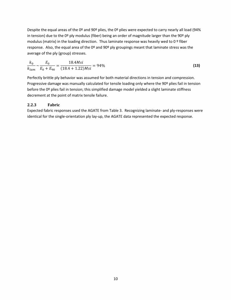
Despite the equal areas of the 0º and 90º plies, the 0º plies were expected to carry nearly all load (94% in tension) due to the 0º ply modulus (fiber) being an order of magnitude larger than the 90º ply modulus (matrix) in the loading direction. Thus laminate response was heavily wed to 0 º fiber response. Also, the equal area of the 0º and 90º ply groupings meant that laminate stress was the average of the ply (group) stresses.

𝑘0𝑘𝑙𝑎𝑚

~𝐸0

𝐸0 + 𝐸90=

18.4𝑀𝑠𝑖(18.4 + 1.22)𝑀𝑠𝑖

= 94% (13)

Perfectly brittle ply behavior was assumed for both material directions in tension and compression. Progressive damage was manually calculated for tensile loading only where the 90º plies fail in tension before the 0º plies fail in tension; this simplified damage model yielded a slight laminate stiffness decrement at the point of matrix tensile failure.

2.2.3 Fabric Expected fabric responses used the AGATE from Table 3. Recognizing laminate- and ply-responses were identical for the single-orientation ply lay-up, the AGATE data represented the expected response.

11

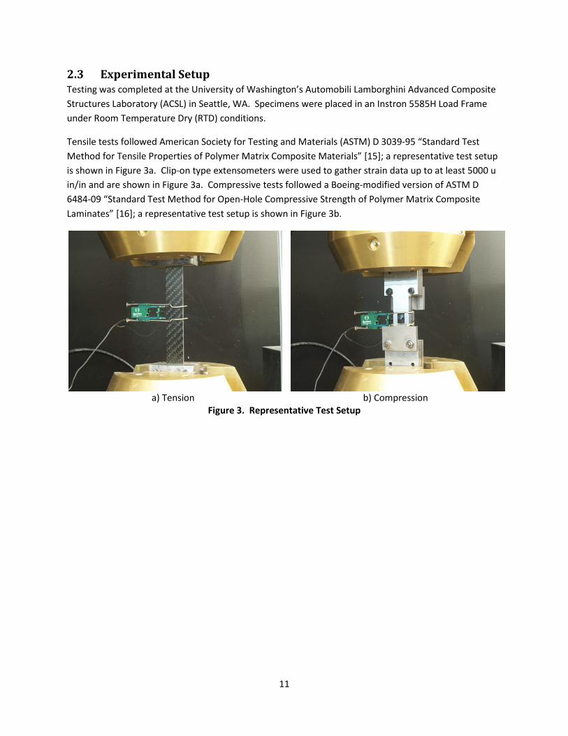
2.3 Experimental Setup Testing was completed at the University of Washington’s Automobili Lamborghini Advanced Composite Structures Laboratory (ACSL) in Seattle, WA. Specimens were placed in an Instron 5585H Load Frame under Room Temperature Dry (RTD) conditions.

Tensile tests followed American Society for Testing and Materials (ASTM) D 3039-95 “Standard Test Method for Tensile Properties of Polymer Matrix Composite Materials” [15]; a representative test setup is shown in Figure 3a. Clip-on type extensometers were used to gather strain data up to at least 5000 u in/in and are shown in Figure 3a. Compressive tests followed a Boeing-modified version of ASTM D 6484-09 “Standard Test Method for Open-Hole Compressive Strength of Polymer Matrix Composite Laminates” [16]; a representative test setup is shown in Figure 3b.

a) Tension

b) Compression

Figure 3. Representative Test Setup

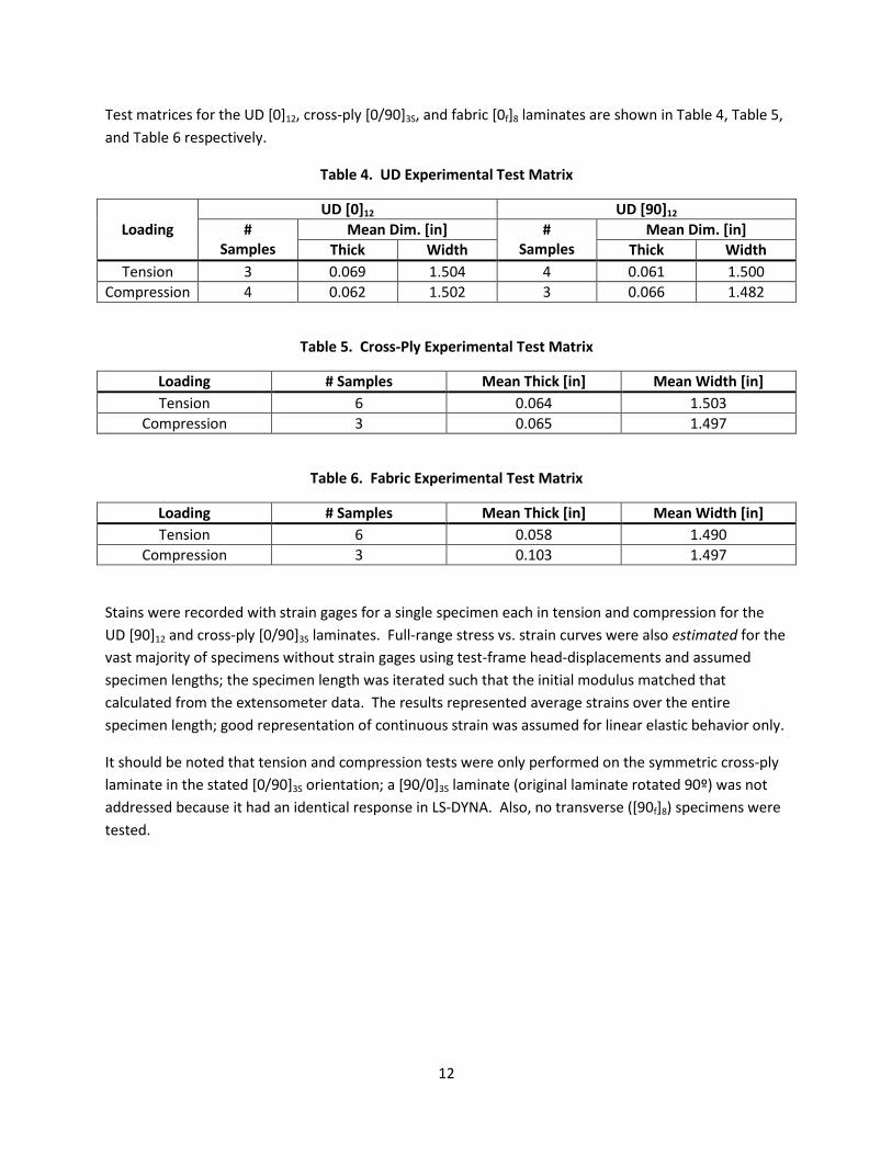
12

Test matrices for the UD [0]12, cross-ply [0/90]3S, and fabric [0f]8 laminates are shown in Table 4, Table 5, and Table 6 respectively.

Table 4. UD Experimental Test Matrix

UD [0]12 UD [90]12 Loading #

Samples Mean Dim. [in] #

Samples Mean Dim. [in]

Thick Width Thick Width Tension 3 0.069 1.504 4 0.061 1.500

Compression 4 0.062 1.502 3 0.066 1.482

Table 5. Cross-Ply Experimental Test Matrix

Loading # Samples Mean Thick [in] Mean Width [in] Tension 6 0.064 1.503

Compression 3 0.065 1.497

Table 6. Fabric Experimental Test Matrix

Loading # Samples Mean Thick [in] Mean Width [in] Tension 6 0.058 1.490

Compression 3 0.103 1.497

Stains were recorded with strain gages for a single specimen each in tension and compression for the UD [90]12 and cross-ply [0/90]3S laminates. Full-range stress vs. strain curves were also estimated for the vast majority of specimens without strain gages using test-frame head-displacements and assumed specimen lengths; the specimen length was iterated such that the initial modulus matched that calculated from the extensometer data. The results represented average strains over the entire specimen length; good representation of continuous strain was assumed for linear elastic behavior only.

It should be noted that tension and compression tests were only performed on the symmetric cross-ply laminate in the stated [0/90]3S orientation; a [90/0]3S laminate (original laminate rotated 90º) was not addressed because it had an identical response in LS-DYNA. Also, no transverse ([90f]8) specimens were tested.

13

2.4 Experimental Results

2.4.1 UD Results from the [0]12 coupon tests, Figure 4a, aligned well with the expected linear elastic results. The [90]12 experimental results, Figure 4b, deviated noticeably from the calculated linear stress-strain curve. Since nonlinear behavior is characteristic of matrix-dominated laminates, deviations from the linear-elastic assumption were anticipated.

a) Longitudinal b) Transverse

Figure 4. Baseline UD Stress vs. Strain – All Specimens

Results for the [0]12 (longitudinal) and [90]12 (transverse) laminates are provided in Table 7 and Table 8 respectively. Each table lists peak force, elastic modulus, strength, and peak energy for the experimental and expected results.

Table 7. [0]12 UD Baseline Results – Experimental & Theory

-300

-200

-100

0

100

200

300

400

-15,000 -10,000 -5,000 0 5,000 10,000 15,000 20,000

Lam

inat

e St

ress

[ksi

]

Strain [u in/in]

Expected [0]12Test-Avg. Strain

-40

-35

-30

-25

-20

-15

-10

-5

0

5

10

-40,000 -30,000 -20,000 -10,000 0 10,000

Lam

inat

e St

ress

[ksi

]Strain [u in/in]

Expected [90]12

Test-Avg. Strain

Loading Quantity Force Modulus Strength Energy[lbf] [Msi] [ksi] [lbf*in]

Tension Test Mean 32,025 18.84 309.8 2,664Test Coeff. Var. 9% 5% 11% 18%

Expected 33,016 18.40 319.0 2,929Error -3% 2% -3% -9%

Compression Test Mean -13,375 16.29 -143 492Test Coeff Var. -14% 6% -15% 30%

Expected -19,928 16.50 -213 834Error -33% -1% -33% -41%

14

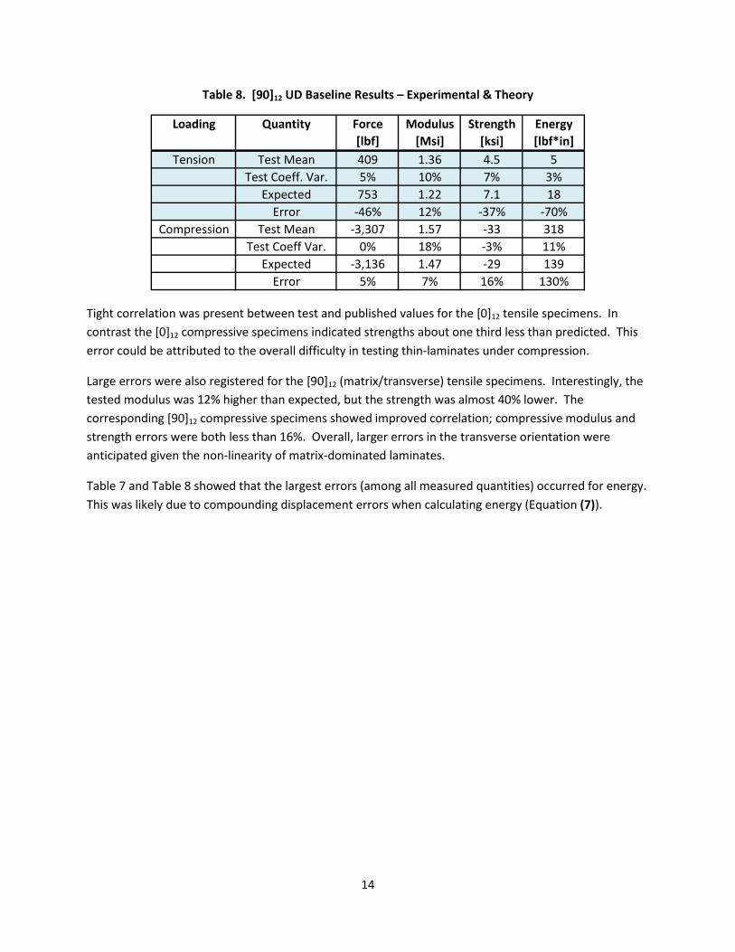
Table 8. [90]12 UD Baseline Results – Experimental & Theory

Tight correlation was present between test and published values for the [0]12 tensile specimens. In contrast the [0]12 compressive specimens indicated strengths about one third less than predicted. This error could be attributed to the overall difficulty in testing thin-laminates under compression.

Large errors were also registered for the [90]12 (matrix/transverse) tensile specimens. Interestingly, the tested modulus was 12% higher than expected, but the strength was almost 40% lower. The corresponding [90]12 compressive specimens showed improved correlation; compressive modulus and strength errors were both less than 16%. Overall, larger errors in the transverse orientation were anticipated given the non-linearity of matrix-dominated laminates.

Table 7 and Table 8 showed that the largest errors (among all measured quantities) occurred for energy. This was likely due to compounding displacement errors when calculating energy (Equation (7)).

Loading Quantity Force Modulus Strength Energy[lbf] [Msi] [ksi] [lbf*in]

Tension Test Mean 409 1.36 4.5 5Test Coeff. Var. 5% 10% 7% 3%

Expected 753 1.22 7.1 18Error -46% 12% -37% -70%

Compression Test Mean -3,307 1.57 -33 318Test Coeff Var. 0% 18% -3% 11%

Expected -3,136 1.47 -29 139Error 5% 7% 16% 130%

15

2.4.2 Cross-Ply Table 9. Cross-Ply Baseline Results – Experimental & Theory

Table 9 provides peak force, elastic modulus, failure strength, failure strain, and peak energy for the experimental and theoretical (expected) results.

The elastic modulus showed good correlation in both tension and compression between test and theory. This confirmed the prediction that laminate response was the average of the 0º (fiber/1-dir) and 90º (matrix/2-dir) ply moduli for this simple, symmetric, cross-ply lay-up (Equation (4)). Results also showed a tensile modulus higher than the compressive modulus.

Small laminate strength errors also supported the prediction that laminate stress was the average of the 0º and 90º ply groups. The small tensile strength error (-1%) was likely aided by the well-defined linear-elastic brittle response of fibers. Alternately, the difficulty in completing thin composite compression tests and the slight non-linearity in fiber compression likely explained the larger compressive strength error (-12%). At a macroscopic level, laminate tensile strength exceeded compressive strength as expected. Overall, the laminate response indicated a qualitatively linear-elastic response with brittle failure.

Reasonable correlation was also achieved for tensile and compressive energy. The 16% maximum error was higher than either the modulus or strength errors; however, this was due to the integration of displacement errors when calculating energy (Equation (7)).

Loading Quantity Force Modulus Strength Strain Energy[lbf] [Msi] [ksi] [u in/in] [lbf*in]

Tension Test Mean 15,096 10.58 157 15,208 1,008Test Coeff. Var. 11% 3% 7% Single S/G 29%

Expected 15,089 9.81 160 17,337 1,140Error 0% 8% -1% -12% -12%

Compression Test Mean -10,006 8.84 -102 -11,359 509Test Coeff Var. -15% 3% -11% Single S/G 19%

Expected -11,291 8.99 -116 -12,909 441Error -11% -2% -12% -12% 16%

16

Full range stress vs. strain curves are shown in Figure 5 for the cross-ply laminate. Test curves reflected strain gage data and indicated a laminate response qualitatively similar to theory/expectation. However, both the tensile and compressive experimental curves displayed some measure of non-linearity at strains in excess of 5000 u in/in and were alternatively stiffer and softer respectively than predicted.

Figure 5. Baseline Cross-Ply Stress vs. Strain – Strain Gage Specimens Only

-150

-100

-50

0

50

100

150

200

-15,000 -10,000 -5,000 0 5,000 10,000 15,000 20,000

Lam

inat

e St

ress

[ksi

]

Strain [u in/in]

Expected

Test-S/G

17

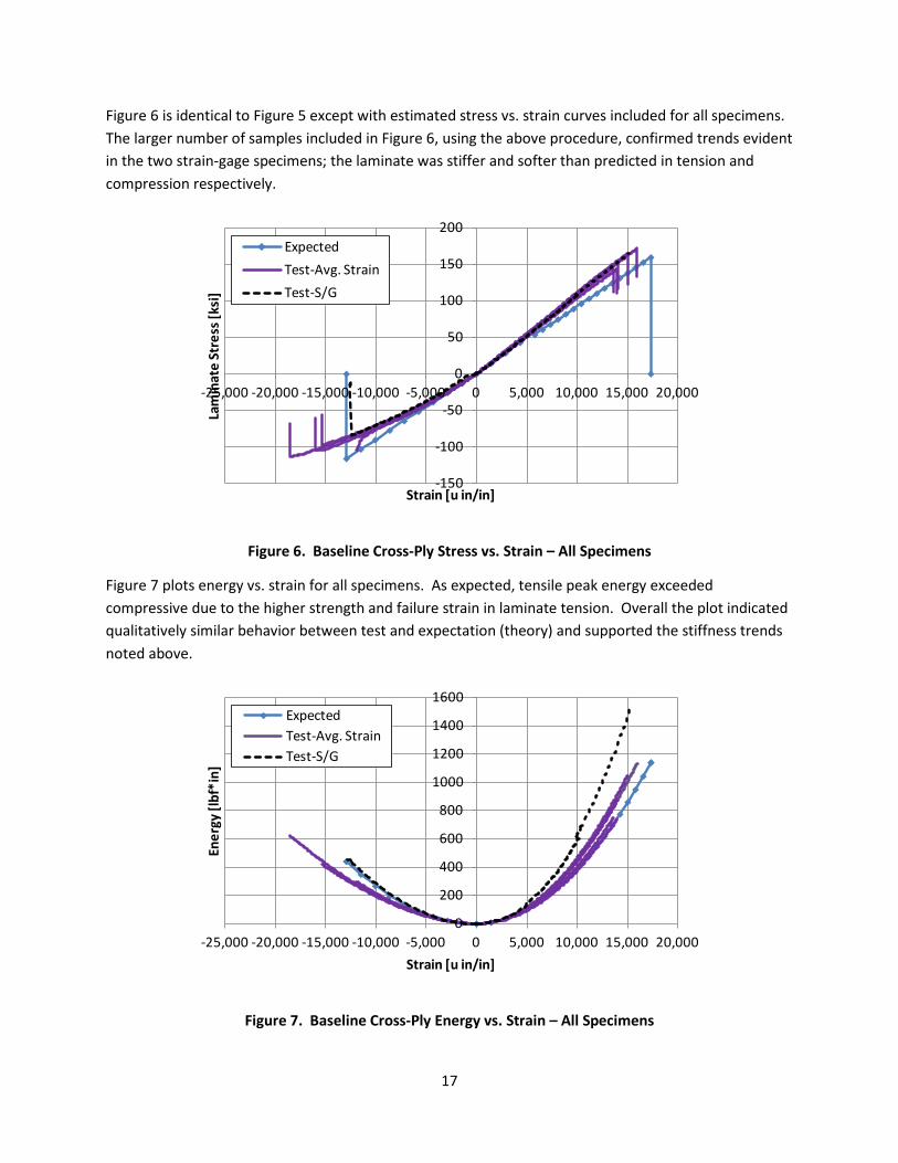
Figure 6 is identical to Figure 5 except with estimated stress vs. strain curves included for all specimens. The larger number of samples included in Figure 6, using the above procedure, confirmed trends evident in the two strain-gage specimens; the laminate was stiffer and softer than predicted in tension and compression respectively.

Figure 6. Baseline Cross-Ply Stress vs. Strain – All Specimens

Figure 7 plots energy vs. strain for all specimens. As expected, tensile peak energy exceeded compressive due to the higher strength and failure strain in laminate tension. Overall the plot indicated qualitatively similar behavior between test and expectation (theory) and supported the stiffness trends noted above.

Figure 7. Baseline Cross-Ply Energy vs. Strain – All Specimens

-150

-100

-50

0

50

100

150

200

-25,000 -20,000 -15,000 -10,000 -5,000 0 5,000 10,000 15,000 20,000

Lam

inat

e St

ress

[ksi

]

Strain [u in/in]

ExpectedTest-Avg. StrainTest-S/G

0

200

400

600

800

1000

1200

1400

1600

-25,000 -20,000 -15,000 -10,000 -5,000 0 5,000 10,000 15,000 20,000

Ener

gy [l

bf*i

n]

Strain [u in/in]

ExpectedTest-Avg. StrainTest-S/G

18

Finally, Figure 8 shows load vs. displacement curves for all specimens. As witnessed with the preceding plots, the laminate was stiffer in tension and softer in compression than predicted, tensile capability exceeded compressive, and non-linearity was most pronounced in the compressive specimens.

Figure 8. Baseline Cross-Ply Load vs. Displacement – All Specimens

Following is a summary of the baseline cross-ply behavior (tested and expected):

• Laminate moduli and stresses were the average of the ply moduli and stresses for this simple cross-ply lay-up.

• The 0º plies carried the vast majority of load and thus defined laminate failure points. • Laminate tensile strength and capability exceeded compressive. • Material response contained slight non-linearity in compression; failure was brittle in tension

and compression. • The laminate was slightly stiffer (larger modulus) in tension than in compression. • More energy was stored/absorbed in tension than compression.

-15000

-10000

-5000

0

5000

10000

15000

20000

-0.15 -0.10 -0.05 0.00 0.05 0.10 0.15 0.20

Forc

e [lb

f]

Displ. [in]

ExpectedTestTest-S/G

19

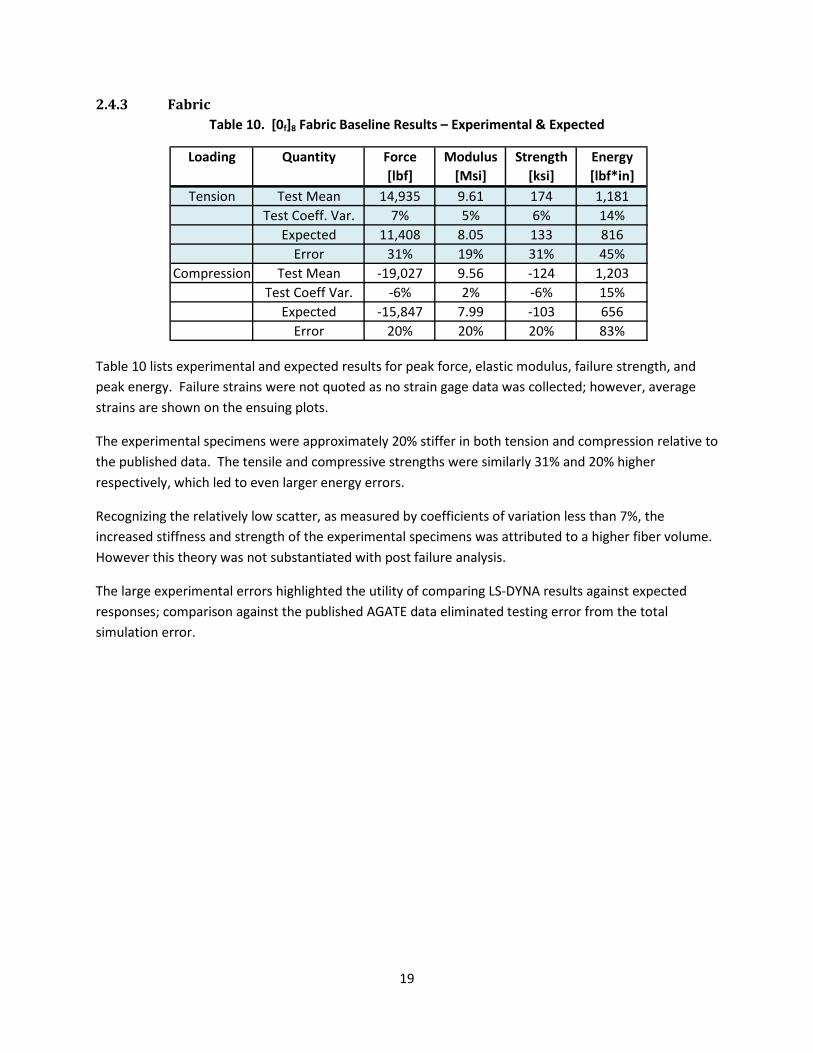
2.4.3 Fabric Table 10. [0f]8 Fabric Baseline Results – Experimental & Expected

Table 10 lists experimental and expected results for peak force, elastic modulus, failure strength, and peak energy. Failure strains were not quoted as no strain gage data was collected; however, average strains are shown on the ensuing plots.

The experimental specimens were approximately 20% stiffer in both tension and compression relative to the published data. The tensile and compressive strengths were similarly 31% and 20% higher respectively, which led to even larger energy errors.

Recognizing the relatively low scatter, as measured by coefficients of variation less than 7%, the increased stiffness and strength of the experimental specimens was attributed to a higher fiber volume. However this theory was not substantiated with post failure analysis.

The large experimental errors highlighted the utility of comparing LS-DYNA results against expected responses; comparison against the published AGATE data eliminated testing error from the total simulation error.

Loading Quantity Force Modulus Strength Energy[lbf] [Msi] [ksi] [lbf*in]

Tension Test Mean 14,935 9.61 174 1,181Test Coeff. Var. 7% 5% 6% 14%

Expected 11,408 8.05 133 816Error 31% 19% 31% 45%

Compression Test Mean -19,027 9.56 -124 1,203Test Coeff Var. -6% 2% -6% 15%

Expected -15,847 7.99 -103 656Error 20% 20% 20% 83%

20

Not addressed in Table 10 were the failure strains or transverse fabric properties; Table 11 lists expected results for both. Unlike the UD tape material system, fabric properties were of the same order for the two material directions and loading orientations. Similar fabric tensile and compressive failure strains were expected to minimize MAT54 simulation errors caused by the limitation (introduced later) of a single material 2-direction failure strain.

Table 11. Fabric Longitudinal (1-dir) and Transverse (2-dir) Expected Properties

Figure 9 shows full range stress vs. strain curves for the [0f]8 fabric laminate. In the absence of strain gage data, the curves were estimated from test frame head displacements and assumed specimen lengths (as was done for the other laminates). Consistent with Table 10 the test specimens were stiffer and stronger in both tension and compression.

Figure 9. Baseline [0f]8 Fabric Stress vs. Strain – All Specimens

Material Loading Modulus Strength StrainDirection [Msi] [ksi] [u in/in]

Tension 8.05 133 16,522Compression 7.99 -103 -12,891

Tension 7.94 112 14,106Compression 7.76 -102 -13,144

Long./1-dir

Tran./2-dir

-150

-100

-50

0

50

100

150

200

-20,000 -10,000 0 10,000 20,000

Lam

inat

e St

ress

[ksi

]

Strain [u in/in]

Expected-Long

Test-Avg. Strain

21

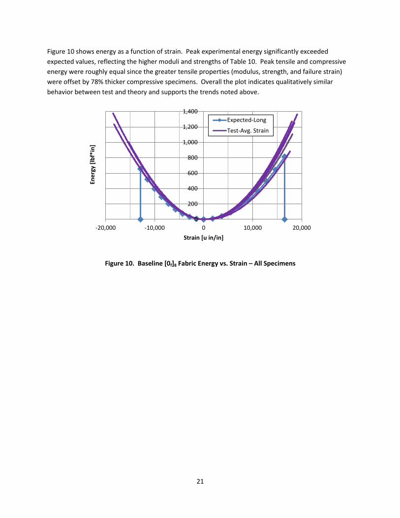
Figure 10 shows energy as a function of strain. Peak experimental energy significantly exceeded expected values, reflecting the higher moduli and strengths of Table 10. Peak tensile and compressive energy were roughly equal since the greater tensile properties (modulus, strength, and failure strain) were offset by 78% thicker compressive specimens. Overall the plot indicates qualitatively similar behavior between test and theory and supports the trends noted above.

Figure 10. Baseline [0f]8 Fabric Energy vs. Strain – All Specimens

0

200

400

600

800

1,000

1,200

1,400

-20,000 -10,000 0 10,000 20,000

Ener

gy [l

bf*i

n]

Strain [u in/in]

Expected-Long

Test-Avg. Strain

22

Figure 11 confirms the effect of specimen geometry (thickness) on both energy and force. Unlike stress and strain, the load-displacement curves in Figure 11 were dependent on geometry and showed the compressive stiffness (curve slope) far exceeding the tensile. This figure also showed a measure of non-linearity in all of the compressive specimens.

Figure 11. Baseline [0f]8 Fabric Load vs. Displacement – All Specimens

Baseline fabric behavior is summarized below:

• Laminate failure was brittle in tension and compression; slight non-linearity was present in compression.

• Experimental test specimens were significantly stiffer and stronger than expected from the published data.

• Tensile and compressive properties were of the same order for both fabric material directions; however, tensile properties generally exceeded compressive and longitudinal (fabric waft) slightly exceeded transverse (fabric weft).

-20,000

-15,000

-10,000

-5,000

0

5,000

10,000

15,000

20,000

-0.15 -0.10 -0.05 0.00 0.05 0.10 0.15 0.20Forc

e [lb

f]

Displ. [in]

Expected-LongTest

23

Figure 12 plots stress vs. strain for the (0/90)3S cross-ply and (0f)8 fabric specimens. The results were very similar recognizing similar fiber volumes between each laminate and identical fiber and matrix constituents between the UD and fabric material forms.

Figure 12. Baseline Fabric and Cross-Ply Stress vs. Strain – All Specimens

-150

-100

-50

0

50

100

150

200

-20000 -10000 0 10000 20000

Lam

inat

e St

ress

[ksi

]

Strain [u in/in]

Cross-PlyFabric

24

3. Numerical Simulations The purpose of this section was to develop single-element simulations with the LS-DYNA MAT54 material model. Prior to the numerical setup and results, a review of the MAT54 material model is provided to familiarize the reader with the material model.

3.1 LS-DYNA MAT54 Material Model

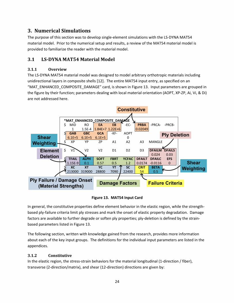
3.1.1 Overview The LS-DYNA MAT54 material model was designed to model arbitrary orthotropic materials including unidirectional layers in composite shells [12]. The entire MAT54 input entry, as specified on an “MAT_ENHANCED_COMPOSITE_DAMAGE” card, is shown in Figure 13. Input parameters are grouped in the figure by their function; parameters dealing with local material orientation (AOPT, XP-ZP, Ai, Vi, & Di) are not addressed here.

Figure 13. MAT54 Input Card

In general, the constitutive properties define element behavior in the elastic region, while the strength-based ply-failure criteria limit ply stresses and mark the onset of elastic property degradation. Damage factors are available to further degrade or soften ply properties; ply-deletion is defined by the strain-based parameters listed in Figure 13.

The following section, written with knowledge gained from the research, provides more information about each of the key input groups. The definitions for the individual input parameters are listed in the appendices.

3.1.2 Constitutive In the elastic region, the stress-strain behaviors for the material longitudinal (1-direction / fiber), transverse (2-direction/matrix), and shear (12-direction) directions are given by:

MID1

XP

V1

TFAIL1.15E-9

XC213000

$MAT_ENHANCED_COMPOSITE_DAMAGE*

$

$

$

$

$

YP

V2

ALPH0.1XT

319000

ZP

V2

SOFT0.57YC

28800

-KF-

A1

D1

FBRT0.5YT

7090

-EC-

AOPT0

A2

D2

YCFAC1.2SC

22400

PRBA0.02049

A3

D3

DFAILT0.0174

CRIT54

-PRCA-

MANGLE

DFAILM0.024

DFAILC-0.0116

BETA0.5

-PRCB-

DFAILS0.03EFS

0

Constitutive

Ply Deletion

Ply Failure / Damage Onset(Material Strengths) Failure CriteriaDamage Factors

ElementDeletion

GAB6.1E+5

RO1.5E-4GBC

6.1E+5

EA1.84E+7

GCA6.1E+5

EB1.22E+6

Shear Weighting

Shear Weighting

25

𝜀11 = 1𝐸1

(𝜎11 − 𝑣12𝜎22) where E1 = EA and 𝑣12 = 𝑃𝑅𝐵𝐴∙𝐸𝐴𝐸𝐵

(14)

𝜀22 = 1𝐸2

(𝜎22 − 𝑣21𝜎11) where E2 = EB and 𝑣21 = 𝑃𝑅𝐵𝐴 (15)

2𝜀12 = 1𝐺12

𝜎12 + 𝛼𝜎123 where G12 = GAB and α = ALPH (16)

In Equation (16), the α (ALPH) input parameter is a weighing factor for the nonlinear shear stress term. ALPH cannot be experimentally determined, but needs to be calibrated by trial and error whenever shear is present. GBC and GCA (not listed in the above equations) are the out-of-plane shear moduli.

3.1.3 Ply Failure (Damage Onset) MAT54 uses the Chang-Chang ply-failure criteria [17] to limit ply stresses and mark the onset of ply degradation. Equations (17) through (20) provide the MAT54 Chang-Chang implementation where XT is the ply longitudinal tensile strength, XC is the ply longitudinal compressive strength, YT is the ply transverse tensile strength, YC is the ply transverse compressive strength, and SC is the ply shear strength. These input parameters can be measured through testing of the lamina. Relevant to a unidirectional ply, the longitudinal and transverse strengths would represent fiber and matrix respectively.

𝑒𝑓2 = �𝜎11𝑋𝑡�2

+ 𝛽 �𝜎12𝑆𝑐�2− 1 �

𝑒𝑓2 ≥ 0 failed𝑒𝑓2 < 0 elastic

� (17)

𝑒𝑐2 = �𝜎11𝑋𝑐�2− 1 � 𝑒𝑐

2 ≥ 0 failed𝑒𝑐2 < 0 elastic

� (18)

𝑒𝑚2 = �𝜎22𝑌𝑡�2

+ �𝜎12𝑆𝑐�2− 1 � 𝑒𝑚

2 ≥ 0 failed𝑒𝑚2 < 0 elastic

� (19)

𝑒𝑑2 = �𝜎222𝑆𝑐

�2

+ ��𝑌𝑐

2𝑆𝑐�2− 1�

𝜎22𝑌𝑐

+ �𝜎12𝑆𝑐�2

− 1 �𝑒𝑑2 ≥ 0 𝑓𝑎𝑖𝑙𝑒𝑑

𝑒𝑑2 < 0 𝑒𝑙𝑎𝑠𝑡𝑖𝑐� (20)

ef, ec, em and ed in Equations (17)-(20) are called history variables and they are flags that represent the strength-based failure for each of the four failure modes (fiber tension ef, fiber compression ec, matrix tension em, and matrix compression ed).1

1 Contrary to the equations above the history variables, when written to integration point output variables, unity denotes elastic behavior and zero represents a failed or deleted ply.

26

The shear stress weighing factor β (BETA) allows the user to explicitly define the influence of shear in the tensile fiber mode. A BETA value of one implements the Hashin [18] failure criterion, while a value of zero reduces Equation (17) to the Maximum Stress failure criteria. Selecting the BETA value is a matter of preference, and otherwise can be done by trial and error.

When one of the above conditions is exceeded in a ply within the element, the specified elastic properties for that ply are reduced to zero. The mechanism by which MAT54 applies this elastic property reduction, however, only prevents the failed ply from carrying additional stress rather than reducing the stress to zero or a near zero value. The equation used by MAT54 to determine 1- and 2-direction element stresses in the ith time step provides insight into this mechanism:

�𝜎11𝜎22�𝑖

= �𝜎11𝜎22�𝑖−1

+ �𝐶11 𝐶12𝐶12 𝐶22

�𝑖�∆𝜀11∆𝜀22

�𝑖 (21)

When ply failure occurs in the ith time step, constitutive properties in the stiffness matrix C go to zero, but the stresses from the i-1 time step are non-zero. This leads the failed ply stresses to be constant and unchanged from the stress state just prior to failure. The resulting ‘plastic’ behavior, shown in Figure 14, occurs when the strength is reached before a failure strain (‘DFAIL’ in Figure 14). Elastic property degradation following failure in MAT54 works in this way rather than degrading properties in the elastic Equations (14)-(16), which would result in a reduced or zero stress state in a failed ply. Therefore the “failure criteria” label is slightly misleading as a ply does not truly fail (cease load carrying capability) until deleted by strain-based measures.

Figure 14. Typical Ply Stress-Strain Behavior

ε

σFu

FuE

DFA

IL

= Chang-Chang Strength-Based Ply Failure

= Strain-Based Ply Deletion (typical)

27

3.1.4 Damage Factors The MAT54 FBRT and YCFAC strength reduction parameters are used to degrade the pristine fiber strengths of a ply if compressive matrix failure takes place. This strength reduction simulates damage done to the fibers from the failed matrix and it is applied using the following equations:

𝑋𝑇reduced = 𝑋𝑇 ∙ 𝐹𝐵𝑅𝑇 (22)

𝑋𝐶reduced = 𝑌𝐶 ∙ 𝑌𝐶𝐹𝐴𝐶 (23)

The FBRT parameter defines the percentage of the pristine fiber strength that is left following compressive matrix failure, therefore its value should be in the range zero to one. The YCFAC parameter uses the pristine matrix strength YC to determine the damaged compressive fiber strength, which means that the upper limit of YCFAC is XC/YC. The input value for the two parameters FBRT and YCFAC cannot be measured experimentally and must be determined by trial and error.

The SOFT parameter is a strength reduction factor for crush simulations. This parameter reduces the strength of the elements immediately ahead of the crush front in order to simulate damage propagating from the crush front. The strength degradation is applied to four of the material strengths as follows:

{𝑋𝑇,𝑋𝐶,𝑌𝑇,𝑌𝐶}reduced = {𝑋𝑇,𝑋𝐶,𝑌𝑇,𝑌𝐶} ∙ 𝑆𝑂𝐹𝑇 (24)

Reducing material strengths using SOFT allows for greater stability to achieve stable crushing by softening the load transition from the active row of elements to the next. The SOFT parameter is active within the range [0,1], where a SOFT value of one indicates that the elements at the crush front retain their pristine strength and no softening occurs. Since this parameter cannot be measured experimentally, it must be calibrated by trial and error for crush simulations.

28

3.1.5 Ply Deletion The failure equations described in Equations (17)-(20) provide the maximum stress limit of a ply, and the damage mechanisms described in Equations (22)-(24) reduce the stress limit by a specified value given specific loading conditions. None of these mechanisms, however, cause the ply stress to go to zero.

Instead, there are five critical strain values that may delete a ply and reduce the ply stress to zero. These are the strain to failure values in fiber tension DFAILT, fiber compression DFAILC, the matrix direction DFAILM, ply shear DFAILS, and a combined failure strain parameter called Effective Failure Strain (EFS). It is important to note that in the matrix direction there is only a single failure strain value available for both tension and compression.

Four of the failure strains can be measured through coupon-level tests, but if they are not known, LS-DYNA gives the user the option to employ a generic failure strain parameter. The EFS immediately reduces the ply stresses to zero when the strain in any direction exceeds EFS, which is given by:

𝐸𝐹𝑆 = �43

(𝜀112 + 𝜀11𝜀22 + 𝜀222 + 𝜀122) (25)

A critical EFS value can be calculated for any simulation in advance by predicting 1-, 2-, and 12-strains at element failure and using Equation (25). The default value for EFS is zero, which is interpreted by MAT54 to be numerically infinite.

3.1.6 Element Deletion A MAT54 shell element is deleted once all integration points (plies) have exceeded one of the strain parameters (DFAIL or EFS). Element deletion can also occur when the element becomes highly distorted and requires a very small time step. A minimum time step parameter, TFAIL, removes distorted elements as follows:

TFAIL ≤ 0: No element deletion by time step

0 < TFAIL ≤ 0.1: Element is deleted when its time step is smaller than TFAIL

TFAIL > 0.1: Element is deleted when current time−steporiginal time−step

< TFAIL

Defining TFAIL to be very near or greater than the element time step will cause premature element deletion since the element will violate the TFAIL condition in its initial state.

Unlike the strength-based ply failure criterion in Eqs. (17)-(20), there are no history variables for ply failure due to maximum strains or element deletion due to TFAIL. Therefore it is not possible to distinguish the failure mode that causes element deletion from the simulation results.

29

3.2 LS-DYNA Single Element Simulation Setup

3.2.1 Common Setup LS-DYNA is developed by Livermore Software Technology Corporation (LSTC) and version 971 was used for all simulations. The double-precision solver was selected to avoid numerical instabilities when exploring the extremes of some parameters.

Two material systems were explored in this research; properties for the Toray T700GC-12K-31E/#2510 UD tape and T700SC-12K-50C/#2510 plain-weave fabric are provided in Table 2 and Table 3 respectively. Material properties were entered on the “*MAT_ENHANCED_COMPOSITE_DAMAGE” card. The input card for the UD material system is provided in Figure 13.

All laminates were defined using the “*PART_COMPOSITE” input card, which accepted material, thickness, and orientation (angle) on a ply-by-ply basis. The LS-DYNA Type 16 fully-integrated shell element was used for all simulations.

Figure 15. Single Element Mesh, Boundary Conditions, & Loading

The single four-node shell element was defined using the “*ELEMENT_SHELL” card. The 0.1-in square element and typical boundary conditions are shown in Figure 15. Each laminate was subjected to tension and compression about perpendicular loading axes (i.e. longitudinal and transverse). Rather than modifying either the element connectivity or applied loading, transverse loading was accomplished by rotating a laminate’s plies by 90 degrees. In addition to the longitudinal and transverse boundary conditions shown in Figure 15, all out-of-plane displacements were constrained (Z-axis in the global Coordinate System (CS)).

Tensile and compressive loads were created with enforced displacements at a constant loading rate of 2 in/s at nodes 1 and 4. The time step was chosen to be 50% of the critical time step, which was the maximum value determined by the Courant condition [19]. The baseline time step was therefore 2.846(10-7) seconds.

XY

dyN1

N2 N3

N4

Global CS

1

LaminateCS

dyN1

N2 N3

N4

Long.Tension

[0]12

Long. Compression

[0]12

2

1

2

dyN1

N2 N3

N4dyN1

N2 N3

N4

TransverseTension

[90]12

Transverse Compression

[90]12

2

1

2

LaminateCS

1

30

As a part of this study, loading velocities from 1 in/min to 300 in/s were simulated for the UD laminate only and results remained unchanged throughout the velocity range. Since MAT54 does not have any strain-rate sensitive parameters this result was expected, but will not be discussed further in the results section.

Simulation outputs were post-processed with LSTC LS-PRE/POST software. A batch script was used to identically extract results at three levels of scale for all simulations: element (laminate), integration-point (ply), and node. While the LS-DYNA binary output database (“d3plot” file) contained results in all directions, only relevant data in the loading direction was reported for this study. Data of interest at each integration point were the ply stresses and strains. Net reaction forces at the boundary conditions were recorded for comparison against experimental test results. Displacements and velocities were recorded on the free node 4 to monitor for unstable behavior. Finally, the total energy of the element was recorded. The Chang-Chang history variables (Equations (17)-(20)) were monitored at the ply and element levels.

Given the simplicity of the single element uniaxial loading conditions, many of the MAT54 parameters in Figure 13 were found to have insignificant or no influence on the simulation outcome. These included shear-specific parameters (ALPH, BETA, DFAILS, GAB, and SC), as well as parameters that required special loading conditions (SOFT, FBRT, and YCFAC). The Poisson’s ratio, PRBA, had a negligible effect on the results. Therefore the inactive parameters listed in this paragraph are not discussed again.

In contrast, MAT54 parameters that were capable of significantly changing the stress-strain behavior, energy, or stability of the simulation are discussed in the results section. These parameters typically included the constitutive, strength, and failure strain parameters; the UD section provides a more exhaustive look at the remaining ‘active’ parameters.

The parametric studies used the baseline input decks as the starting point for all simulations; therefore boundary conditions, loading, element definition, etc. were common between the baseline and parametric study simulations. Only a single parameter was varied from the baseline state for each new simulation. Results were not compared against the test data; therefore simulation energy and reaction force were not scaled to match average test specimen geometry as in the baseline section. As a consequence, baseline energy and force plots are different between the “Baseline Behavior” section and the following; however, element and ply stresses were consistent across both sections.

The parametric study encompassed the range of MAT54 parameters shown in Figure 13. Damage parameters (YCFAC, FBRT, & SOFT) were not explored, other than to confirm that these parameters played no role in the simplified model/loading.

Following is laminate-specific simulation setup information.

31

3.2.2 UD Setup The MAT54 entry for the baseline UD simulations was shown in Figure 13. As noted earlier, the failure strains (MAT54 “DFAIL” parameters) were calculated by dividing the material strength by the appropriate modulus (Equations (26)-(28)).

𝐷𝐹𝐴𝐼𝐿𝑇 = 𝑋𝑇𝐸𝐴

(26)

𝐷𝐹𝐴𝐼𝐿𝐶 = 𝑋𝐶𝐸𝐴

(27)

𝐷𝐹𝐴𝐼𝐿𝑀 ={𝑌𝑇,𝑌𝐶}𝐸𝐵

(28)

Unfortunately, the MAT54 material model only accepts a single failure strain to represent both tensile and compressive transverse (matrix) failures. Therefore, Equation (28) shows that DFAILM can be defined using either the tensile or compressive matrix strengths. The higher of the two values (matrix compression “YT”) was initially used to define DFAILM in this study.

The test matrix for the study of MAT54 parameters using the [0]12 UD laminate is given in Table 12. Parameters that exclusively influenced the matrix direction, such as EB, DFAILM, YC and YT, are omitted from this report since they were found to have no influence on the [0]12 simulations in the loading direction.

Table 12. UD [0]12 Parametric Study – Simulation Matrix

Parameter Tension Compression Units EA 0, 9.2, (18.4), 36.8 Msi XT 0, 200, (319), 400 - ksi XC - 0, -50, -100, -200, (-213), -300 ksi DFAILT 0, 0.01, (0.0174), 0.03 - in/in DFAILC - 0, -0.005, -0.01, (-0.0116), -

0.02, -0.03 in/in

EFS (0), 0.001, 0.01, 0.017821 - in/in TFAIL (1.153E-9), 2.835E-7, 2.840E-

7, 2.846E-7 - s

32

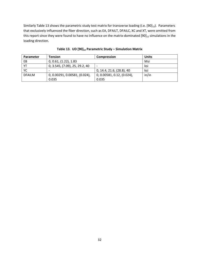
Similarly Table 13 shows the parametric study test matrix for transverse loading (i.e. [90]12). Parameters that exclusively influenced the fiber direction, such as EA, DFAILT, DFAILC, XC and XT, were omitted from this report since they were found to have no influence on the matrix-dominated [90]12 simulations in the loading direction.

Table 13. UD [90]12 Parametric Study – Simulation Matrix

Parameter Tension Compression Units EB 0, 0.61, (1.22), 1.83 Msi YT 0, 3.545, (7.09), 25, 29.2, 40 - ksi YC - 0, 14.4, 21.6, (28.8), 40 ksi DFAILM 0, 0.00291, 0.00581, (0.024),

0.035 0, 0.00581, 0.12, (0.024), 0.035

in/in

33

3.2.3 Cross-Ply Setup The baseline cross-ply simulations began with the LS-DYNA input deck from the UD simulations of the first section. This included the “*MAT_054” material model, loading, boundary conditions, and element geometry. The primary difference for the 12-ply cross-ply laminate was the individual ply-orientations as defined on the LS-DYNA “*PART_COMPOSITE” entry. The loading and boundary conditions are shown in Figure 16; compressive simulations required off-axis (lateral) supports to prevent unconstrained lateral displacement.

Figure 16. LS-DYNA Cross-Ply Simulations – Loading and Boundary Conditions

N2

N1 N4

N3

CompressionTension

XY

Global CS

12

Laminate CS

N2

N1 N4

N3

[0/90]3S [0/90]3S

34

The parametric study used the baseline [0/90]3S cross-ply input decks as the starting point for all simulations. Results were not compared against the test data; therefore simulation energy and reaction forces were not scaled to match average test specimen geometry as in the baseline section. As a consequence, baseline energy and force plots are different between the cross-ply baseline and parametric study sections; however, element and ply stresses were consistent across both sections. Table 14 is the simulation matrix.

Table 14. Cross-Ply Parametric Study – Simulation Matrix

Parameter Tension Compression Units EA 1.2, 9.2, (18.4), 36.8 Msi EB 0.61, (1.22), 18.4 Msi XT 7,160, (319), 479 2, 5, (319) ksi XC 1, 106.5, (213) 106.5, (213), 234.3 ksi YT 3, (7), 28.8, 29.3 1, (7) ksi YC 1, 14.4, (28.8), 57.6 14.4, (28.8), 31.68 ksi DFAILT 0.0087, (0.0174), 0.024,0.025 0.0087, (0.0174), 0.024 in/in DFAILC -0.0058, (-0.0116), -0.01276 in/in DFAILM 0.0058, (0.024), 0.0264 in/in

A single simulation was completed with all plies rotated 90 degrees relative to the baseline configuration to verify that [0/90]3S and [90/0]3S laminates behaved identically in LS-DYNA for this simplified layup.

35

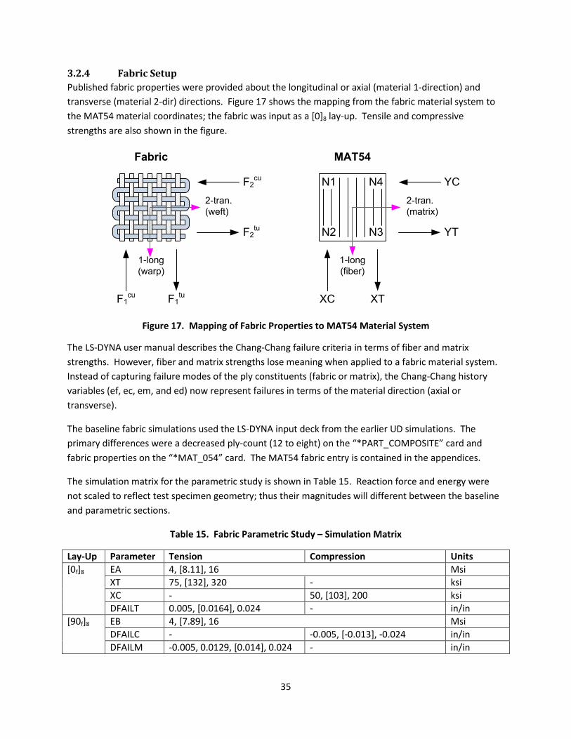
3.2.4 Fabric Setup Published fabric properties were provided about the longitudinal or axial (material 1-direction) and transverse (material 2-dir) directions. Figure 17 shows the mapping from the fabric material system to the MAT54 material coordinates; the fabric was input as a [0]8 lay-up. Tensile and compressive strengths are also shown in the figure.

Figure 17. Mapping of Fabric Properties to MAT54 Material System

The LS-DYNA user manual describes the Chang-Chang failure criteria in terms of fiber and matrix strengths. However, fiber and matrix strengths lose meaning when applied to a fabric material system. Instead of capturing failure modes of the ply constituents (fabric or matrix), the Chang-Chang history variables (ef, ec, em, and ed) now represent failures in terms of the material direction (axial or transverse).

The baseline fabric simulations used the LS-DYNA input deck from the earlier UD simulations. The primary differences were a decreased ply-count (12 to eight) on the “*PART_COMPOSITE” card and fabric properties on the “*MAT_054” card. The MAT54 fabric entry is contained in the appendices.

The simulation matrix for the parametric study is shown in Table 15. Reaction force and energy were not scaled to reflect test specimen geometry; thus their magnitudes will different between the baseline and parametric sections.

Table 15. Fabric Parametric Study – Simulation Matrix

Lay-Up Parameter Tension Compression Units [0f]8 EA 4, [8.11], 16 Msi

XT 75, [132], 320 - ksi XC - 50, [103], 200 ksi DFAILT 0.005, [0.0164], 0.024 - in/in

[90f]8 EB 4, [7.89], 16 Msi DFAILC - -0.005, [-0.013], -0.024 in/in DFAILM -0.005, 0.0129, [0.014], 0.024 - in/in

1-long(warp)

2-tran.(weft)

N2

N1 N4

N3

1-long(fiber)

F1cu F1

tu

F2tu

F2cu

XC XT

YT

YC2-tran.(matrix)

Fabric MAT54

36

3.3 Results

3.3.1 UD Results

3.3.1.1 Baseline The UD single element loaded along the fiber (longitudinal) direction produced the stress-strain curve shown in Figure 18. These results correlated well with the expected linear elastic curve; however, some stiffness error occurred in compression as the MAT54 model only includes a single longitudinal modulus. In contrast, the expected behavior used the published tensile and compressive moduli (Table 2).

Figure 18. Baseline UD [0]12 Stress vs. Strain – Expected & LS-DYNA MAT54

-300

-200

-100

0

100

200

300

400

-15,000 -10,000 -5,000 0 5,000 10,000 15,000 20,000

Lam

inat

e St

ress

[ksi

]

Strain [u in/in]

Expected [0]12MAT54

37

Figure 19 shows parabolic behavior in the energy plot. The parabolic behavior was expected since the stress-strain and load-displacement curves were linear.

Figure 19. Baseline UD [0]12 Energy vs. Strain – Expected & LS-DYNA MAT54

Predictions for the simulation of the UD laminate loaded in the transverse (matrix) direction were not as successful. Figure 20 plots stress versus strain for the UD [90]12 laminate. Simulation results in compression showed the error caused by using a single modulus for both tension and compression.

Figure 20. Baseline UD [90]12 Stress vs. Strain – Expected & LS-DYNA MAT54

0

500

1,000

1,500

2,000

2,500

3,000

3,500

-15,000 -10,000 -5,000 0 5,000 10,000 15,000 20,000

Ener

gy [l

bf*i

n]

Strain [u in/in]

Expected [0]12MAT54

-35

-30

-25

-20

-15

-10

-5

0

5

10

-30,000 -20,000 -10,000 0 10,000 20,000 30,000

Lam

inat

e St

ress

[ksi

]

Strain [u in/in]

Expected [90]12MAT54

38

The error in tension was much more severe. Figure 20 shows an unexpected perfectly plastic region following the linear elastic region and element failure in tension. This plastic region was a consequence of the way MAT54 computes the element stresses after failure using Eq. (21), as illustrated in Figure 14. Recalling that only a single MAT54 failure strain (DFAILM) exists for the material transverse (matrix) direction, the tensile and compressive strains cannot be independently defined. As a consequence, only one strain value satisfied the linear elastic relationship between stress and strain in spite of the existence of two matrix strength parameters (tension and compression).

Since these strengths were different and the matrix failure strain was determined using the compressive value (Equation (28)), the simulation reached the tensile strength before the matrix failure strain. Upon achieving the tensile strength, rather than getting deleted the element continued to plastically strain and carried stress until the failure strain was reached (24,000 u-in/in). This tensile strain value was over four times greater than the expected strain at failure (5800 u-in/in).

Figure 21 shows that the plastic region added a significant amount of energy to the baseline simulation – more than seven times the energy that was expected. Consistent with the plastic stress region, energy increased linearly after exiting the elastic region.

Figure 21. Baseline UD [90]12 Energy vs. Strain – Expected & LS-DYNA MAT54

0

20

40

60

80

100

120

140

160

-30,000 -20,000 -10,000 0 10,000 20,000 30,000

Ener

gy [l

bf*i

n]

Strain [u in/in]

Expected [90]12MAT54

39

Simulation errors are quantified in Table 16 and Table 17 for the UD [0]12 (longitudinal-loaded) and [90]12 (transverse-loaded) laminates respectively.

Table 16. UD [0]12 Baseline Results – Expected & LS-DYNA MAT54

Table 17. UD [90]12 Baseline Results – Expected & LS-DYNA MAT54

In summary, respectable correlation was achieved by the MAT54 [0]12 simulations. However, the MAT54 simulation of the UD [90]12 laminate contained measurable errors in both compression and tension. The relatively minor compressive error was caused by the limitation of a single transverse modulus (rather than one each for tension and compression). Similarly, the severe tensile errors (strain and energy) were caused by the sole material 2-dir (matrix) failure strain (DFAILM) creating an extended plastic region after the strength-based Chang-Chang failure criteria limited ply stresses.

Loading Quantity Force Modulus Strength Energy[lbf] [Msi] [ksi] [lbf*in]

Tension Expected 33,016 18.40 319 2,929MAT54 33,016 18.40 319 2,968Error 0% 0% 0% 1%

Compression Expected -19,928 16.50 -213 834MAT54 -19,926 18.40 -213 744Error 0% 12% 0% -11%

Loading Quantity Force Modulus Strength Energy[lbf] [Msi] [ksi] [lbf*in]

Tension Expected 753 1.22 7.1 18MAT54 651 1.22 7.1 111Error -13% 0% 0% 536%

Compression Expected -3,136 1.47 -29 139MAT54 -2,806 1.22 -29 152Error -11% -17% 0% 10%

40

3.3.1.2 UD Parametric

3.3.1.2.1 UD [0]12 Laminate

3.3.1.2.1.1 Constitutive Parameters Changing the longitudinal (fiber) modulus, EA, affected the single element both in tension and compression since MAT54 did not distinguish compressive and tensile moduli. As one would expect, larger values of EA produced a stiffer stress response from the single element and lower EA values produced a softer response (Figure 22). It should also be noted that the simulation did not run for a zero-valued modulus.

Figure 22. UD [0]12 Parametric Study – Longitudinal/Fiber Modulus (EA) Stress vs. Strain

The failure strain remained the same when changing EA, which caused the element with a smaller modulus to fail at a lower stress value. For the high modulus case, the stress stopped increasing when it reached the tensile strength XT, and continued to plastically deform until the failure strain was reached and the element was deleted. Since this was a fiber-dominated laminate, a plastic response was not expected and was not physically meaningful.

-300

-200

-100

0

100

200

300

400

-0.015 -0.01 -0.005 0 0.005 0.01 0.015 0.02

Stre

ss [k

si]

Strain [in/in]

EA = 36 Msi

EA = 18.4 Msi

EA = 9 Msi

41

3.3.1.2.1.2 Strength Parameters Changing the fiber strengths, XT for tension and XC for compression, changed the peak stress limits of the [0]12 single element simulation. Element stress-strain plots for parametric studies of XT and XC are shown in Figure 23.

Figure 23. UD [0]12 Parametric Study – Longitudinal Strength – Stress vs. Strain

Increasing strength values larger than the baseline values (such as XT = 400 ksi and XC = -300 ksi) changed the results by less than 0.1% from the baseline. The failure strain was reached before the strength for these simulations, which caused element deletion at the same strain as the baseline.

Material strengths set to zero were considered by MAT54 to be numerically infinite, which produced the same results as simulations with increased strengths. Lowering the fiber strength below the baseline value caused the stress to remain constant after achieving the strength until the element was deleted at the given failure strain. Thus raising or lowering the strengths did not achieve the expected results of a linear elastic material because element deletion was strain-based (DFAIL) and ply stresses were limited by the strength-based Chang-Change failure criteria.

0

50

100

150

200

250

300

350

0 0.005 0.01 0.015 0.02

Stre

ss [k

si]

Strain [in/in]

XT ≥ 319 ksi, baselineXT = 200 ksi

-350

-300

-250

-200

-150

-100

-50

0

-0.02 -0.015 -0.01 -0.005 0St

ress

[ksi

]Strain [in/in]

XC ≤ -213 ksi, baselineXC = -100 ksi

(a) (b)

42

A simulation with plasticity in both tension and compression was generated by lowering the tensile and compressive strengths by approximately 100 ksi. The resulting laminate stress-strain curve with plasticity is plotted in Figure 24a, along with the baseline curve and the expected brittle stress-strain result.

Figure 24. UD [0]12 Parametric Study – Reduced Ply Strengths – Stress and Energy vs. Strain

Energy is plotted in Figure 24b. The curves reveal the great difference between the expected results and the results given by MAT54 when plasticity is present. Energy continued to increase linearly after strength-based ply-failure until the failure strain was reached. This more than doubled the tensile energy and was nearly equal to the energy for the baseline strength value.

-300

-200

-100

0

100

200

300

400

-0.02 -0.01 0 0.01 0.02

Stre

ss [k

si]

Strain [in/in]

Baseline [XT = 319, XC = -213] ksiMAT54 [XT = 200, XC = -100] ksiExpected [XT = 200, XC = -100] ksi

0.00

0.05

0.10

0.15

0.20

0.25

-0.02 -0.01 0 0.01 0.02

Ener

gy [J

]

Strain [in/in]

43

3.3.1.2.1.3 Strain Parameters The influence of the strength parameters was not as strong as the longitudinal (fiber) failure strains DFAILT and DFAILC. Varying these parameters showed that increasing the failure strain larger than the baseline caused plasticity until the new failure strain was reached (Figure 25). Decreasing the failure strain caused element deletion before the material strength was reached2.

Figure 25. UD [0]12 Parametric Study – Longitudinal Failure Strains – Stress vs. Strain

2 The time step was decreased for simulations with especially large plastic zones (DFAILC = -0.03 in/in) to simulate the large deformations and avoid minor instabilities.

-400

-350

-300

-250

-200

-150

-100

-50

0

-0.04 -0.03 -0.02 -0.01 0

Stre

ss [k

si]

Strain [in/in]

DFAILC = -0.03 in/inDFAILC = -0.0116, baselineDFAILC = -0.005 in/in

0

50

100

150

200

250

300

350

400

0 0.01 0.02 0.03 0.04

Stre

ss [k

si]

Strain [in/in]

DFAILT = 0.03 in/inDFAILT = 0.0174 in/in, baselineDFAILT = 0.01 in/in

(a) (b)

44

A simulation with plasticity in both tension and compression was generated by using failure strains of ±0.03 in/in. The resulting laminate stress-strain and energy curves are shown along with the expected linear elastic curves in Figure 26. When the failure strain was increased, the simulated MAT54 energy was more than double the total energy expected from linear elastic behavior.

Figure 26. UD [0]12 Parametric Study – Large Longitudinal Failure Strains – Stress vs. Strain

While the effect on the stress-strain curve from changing the failure strains resembled that from changing the material strengths, the plasticity caused by increasing failure strains increased the total energy by a greater amount. When plasticity was introduced by decreasing the strength, the magnitude of the energy added was low because the plastic stress was below the material strength. Adding plasticity by increasing the failure strain added energy at a greater rate since the plastic stress was at the magnitude of the material strength.

A special case arose when DFAILT was set to zero. In this case the fiber tensile strength XT determined deletion in the absence of the fiber tensile failure strain DFAILT. When an element failed in the fiber tension mode, MAT54 implemented a special degradation scheme for the ply stress that reached zero stress after exactly 100 time steps. Once the ply stresses were zero, the element was deleted.

-300

-200

-100

0

100

200

300

400

-0.04 -0.02 0 0.02 0.04

Stre

ss [k

si]

Strain [in/in]

MAT54 [DFAILT = 0.03, DFAILC = -0.03] in/inExpected [DFAILT = 0.03, DFAILC = -0.03] in/in

0

0.1

0.2

0.3

0.4

0.5

0.6

0.7

-0.04 -0.02 0 0.02 0.04

Ener

gy [J

]

Strain [in/in]

45

Figure 27. UD [0]12 Parametric Study – DFAILT = 0 – Stress vs. Strain

The stress degradation when DFAILT is zero is shown in Figure 27. This special case was only applicable to DFAILT and did not work for DFAILC or DFAILM. For instance, using a zero-valued DFAILC immediately terminated the simulation since the maximum failure strain was interpreted to have been violated upon initiation of the simulation. Furthermore, when DFAILT was set to zero but the loading case was not tension in the fiber direction (e.g. fiber compression, matrix tension, matrix compression) the special case shown in Figure 27 did not apply.

0

50

100

150

200

250

300

350

0 0.005 0.01 0.015 0.02

Stre

ss [k

si]

Strain [in/in]

DFAILT = 0.0174, baselineDFAILT = 0

0

50

100

150

200

250

300

350

0.0172 0.0174 0.0176

Stre

ss [k

si]

Strain [in/in]

46

Figure 28. UD [0]12 Parametric Study – EFS – Stress vs. Strain

Determining the effect of the EFS parameter required determination of the critical EFS value for this material system. This was done by the 1- 2- and 12-strains at failure in Eq. (25). The resulting critical EFS value was 0.0178 in/in, which was the effective strain at failure. Using an EFS value less than the critical value caused the element to be deleted at a lower strain as shown in Figure 28. Values higher than the critical value did not change the results. The default value of EFS was zero, which was considered by MAT54 to be numerically infinite. The critical EFS can be determined for any simulation by calculating the EFS at the point of failure. Only values below the critical EFS will influence the simulation results.

0

50

100

150

200

250

300

350

0 0.005 0.01 0.015 0.02 0.025 0.03

Stre

ss [k

si]

Effective Strain [in/in]

EFS ≥ 0.01782 in/in, baselineEFS = 0.01 in/inEFS = 0.005 in/in

47

3.3.1.2.1.4 Element Deletion The MAT54 time step size criteria, affecting element deletion, was also examined. Altering TFAIL such that it was greater than the element time step caused early element deletion. This effect can only be seen by using TFAIL values that are only slightly larger than the element time step (Figure 29). Implementing values any larger than this eliminated the element at the onset of the simulation. A TFAIL value that was two orders of magnitude smaller than the element time step was chosen for the baseline in order to prevent such error.

Figure 29. UD [0]12 Parametric Study – Time Step Criteria TFAIL – Stress vs. Strain

0

50

100

150

200

250

300

350

0 0.005 0.01 0.015 0.02 0.025 0.03

Stre

ss [k

si]

Strain [in/in]

TFAIL = 1.153E-9 s, baselineTFAIL = 2.835E-7 sTFAIL = 2.84E-7 s

48

3.3.1.2.2 UD [90]12 Laminate

3.3.1.2.2.1 Constitutive Parameters

Figure 30. UD [90]12 Parametric Study – Transverse/Matrix Modulus (EB) Stress vs. Strain

Changing the matrix modulus, EB, had the same effect on the [90]12 laminate as changing the fiber modulus on the [0]12 laminate. As shown in Figure 30, raising EB yielded a stiffer response and lowering it caused a softer response, both in tension and compression. It should also be noted that the simulation did not run for a zero-valued modulus.

Figure 30 also highlighted the overarching element behavior noted in Figure 14; independent of the modulus, element deletion was defined by the matrix failure strain DFAILM (0.024 in/in), while ply/element stress was limited by the Chang-Chang failure criteria (reduced to the ply strengths under the simplified loading). This led to large plastic strain regions in cases where the ply strength was reached before the failure strain.

-30

-20

-10

0

10

-0.03 -0.02 -0.01 0 0.01 0.02 0.03

Stre

ss [k

si]

Strain [in/in]

EB = 1.8 MsiEB = 1.22 Msi, baselineEB = 0.61 Msi

49

3.3.1.2.2.2 Strength Parameters The transverse (matrix) strengths, YT and YC for tension and compression respectively, determined the peak stress limits of the [90]12 single element as shown in Figure 31 and Figure 32. The effect of these strengths was similar to the effect of the fiber strengths for the [0]12 laminate. Values greater than or equal to 28.8 ksi for either strength yielded linear elastic behavior, since the matrix failure strain DFAILM deleted the element before higher strengths were obtained.

Figure 31. UD [90]12 Parametric Study – Transverse Tensile Strength (YT) Stress vs. Strain

Figure 32. UD [90]12 Parametric Study – Transverse Compressive Strength (YC) Stress vs. Strain

0

5

10

15

20

25

30

35

0 0.005 0.01 0.015 0.02 0.025 0.03

Stre

ss [k

si]

Strain [in/in]

YT ≥ 28.8 ksiYT = 25 ksiYT = 7.09 ksi, baselineYT = 3.545 ksi

-35

-30

-25

-20

-15

-10

-5

0

-0.03 -0.025 -0.02 -0.015 -0.01 -0.005 0

Stre

ss [k

si]

Strain [in/in]

YC ≥ 28.8 ksi, baselineYC = 14.4 ksi

50

Strength values beyond 28.8 ksi initiated the Chang-Chang failure criteria, which limited ply stresses to the ply strengths under the simplified loading. A region of constant/plastic stress then extended until the failure strain was reached and the element deleted. A zero value for either strength parameter was considered by MAT54 to be numerically infinite; the DFAILM failure strain deleted the element in these cases.

3.3.1.2.2.3 Strain Parameters

Figure 33. UD [90]12 Parametric Study – Transverse Failure Strain (DFAILM) Stress vs. Strain

Changes in DFAILM had a very strong influence on the [90]12 simulations. Lower values underestimated the compressive matrix strength, shown in Figure 33, while increasing DFAILM such that it was larger than the baseline (0.024 in/in) caused an elongation of the plastic region in tension and the introduction of one in compression.

Choosing a zero value for DFAILM caused MAT54 to consider it to be numerically infinite. Therefore no matrix-direction failure strain was active (typically required to delete a ply) and the element was eventually deleted for violating the minimum time step TFAIL. Element deletion occurred at high strain values of 1 in/in and -4 in/in in tension and compression for the default value.

-4 -2 0 2 4

x 104

-30

-25

-20

-15

-10

-5

0

5

10

Strain [µin/in]

Stre

ss [k

si]

a) Element Stress vs. Strain

-4 -2 0 2 4

x 104

0

0.1

0.2

0.3

0.4

0.5

0.6

Strain [µin/in]

Ener

gy [l

b f*in]

b) Energy vs. Strain

DFAILM = 0.024DFAILM = 0.0058DFAILM = 0.035

51

The DFAILM parametric study also afforded an opportunity to revisit selection of the baseline value, which was chosen to coincide with the matrix compressive strength (YC). However, it equally well could have been chosen to coincide with matrix tensile strength (YT). Figure 34 plots stress and energy versus strain for the baseline (0.024 in/in) and YT-based (0.0058 in/in) DFAILM values. While the former showed a large gain in energy, the latter yielded a large loss in energy. The tensile-based value (0.0058 in/in) also showed large strain-to-failure errors in both tension and compression; this contrasted with the compression-based value that only showed large tensile strain error.

Figure 34. UD [90]12 Parametric Study – Transverse Failure Strain (DFAILM) Stress vs. Strain

-3 -2 -1 0 1 2 3

x 104

-30

-25

-20

-15

-10

-5

0

5

10

Strain [µin/in]

Stre

ss [k

si]

a) Element Stress vs. Strain

-3 -2 -1 0 1 2 3

x 104

0

0.05

0.1

0.15

0.2

0.25

0.3

Strain [µin/in]

Ener

gy [l

b f*in]

b) Energy vs. Strain

ExpectedDFAILM = 0.024 (YC/EB)DFAILM = 0.0058 (YT/EB)

52

Simulation errors for both cases are listed in Table 18; neither the tensile (YT) nor compressive (YC) strength based DFAILM value displayed improved results over the other. Thus the DFAILM matrix-strain parameter cannot be tailored to give ideal results like the DFAILT and DFAILC fiber strains and will always cause some error. This must be taken into account when using MAT54 to model a composite material system.

Table 18. [90]12 Parametric Study – Matrix Strain (DFAILM) Error Summary

Quantity Units ExpectedBaseline (YC/EB) YT/EB Expected

Baseline (YC/EB) YT/EB

DFAILM u in/in - 24,000 5,811 - 24,000 5,811Strength ksi 7.09 7.09 7.08 -28.8 -28.8 -7.07

Strength Error - - 0% 0% - 0% -75%Strain u in/in 5,811 23,988 5,800 -19,592 -23,985 -5,795

Strain Error - - 313% 0% - 22% -70%Energy lbf·in 0.016 0.120 0.016 0.223 0.273 0.016

Energy Error - - 635% 0% - 22% -93%

Tension Compression

53

3.3.1.3 Summary Single element LS-DYNA simulations of [0]12 and [90]12 UD laminates with the material model MAT54 revealed the failure mechanisms, post-failure behavior, and critical parameters of this model.

Most prominent among the results was identifying full-range ply stress-strain behavior. Contrary to initial expectations, the strength-based Chang-Chang failure criteria set ply maximum stresses, rather than deleting the ply; one of the ply- or element-deletion parameters was required to end ply load carrying capability – typically the ply failure strains.

This behavior meant that pronounced plastic regions occurred when the Chang-Chang failure criteria was reached prior to the DFAIL failure strains. The effect of failure strain on ply stress-strain behavior is shown in Figure 35 where “Fu” and “E” are the strength and modulus respectively. Simulation results also showed that changing the material strengths has less of an effect on the total simulation energy than changing the failure strains parameters.

Figure 35. Ply Stress-Strain Behavior as Function of DFAIL Failure Strain

Therefore the failure strains (either the three DFAIL values or EFS) should always be defined; otherwise ply and element deletion will solely depend on the TFAIL element time-step size criteria. The DFAIL failure strains should also be set coincident (i.e. quotient of strength and modulus) with corresponding ply strengths to prevent ply plasticity – an attribute not typically associated or desired with brittle orthotropic materials.

= Chang-Chang Strength-Based Ply Failure = Strain-Based Ply Deletion (typical)

ε

σFu

FuE

DFA

IL

ε

σFu

FuEDFAIL =

ε

σFu

FuE

DFA

IL

Low Failure Strain Coincident Failure Strain High Failure Strain

54

Unfortunately, accomplishing the above was hampered by a MAT54 limitation. Only a single transverse/matrix failure strain parameter (DFAILM) existed to represent both tensile and compressive failures, whereas both the DFAILT (tensile) and DFAILC (compressive) parameters were available for longitudinal/fiber strains. As the matrix tensile strength was four times the compressive strength for the UD material system selected in this study, it was not possible to obtain results without error in the transverse direction. However, results showed that DFAILM calculated from the transverse compressive strength caused less error than using the transverse tensile strength for the selected material system.

It should be noted that the DFAILM limitation was not expected to be as detrimental for real-world laminates with mixed orientation plies. When mixed- or cross-plies are present, the fibers will carry the majority of load and matrix-based force and energy errors will be masked. However, poor element failure strain correlation is still expected, which also means failed elements linger in more complex simulations without getting deleted. Both of these predictions were confirmed in the cross-ply study of the following section.

Another MAT54 limitation led to further (though smaller) simulation error – a single elastic modulus to represent both tensile and compressive stiffness. For example, the fiber modulus and matrix tensile moduli were 12% and -17% greater and smaller than their compressive counterparts respectively for the selected material system.

Based on the results of this cross-ply MAT54 parametric study, the following enhancements are recommended for the LS-DYNA MAT54 material to improve simulation results without large detriments to computational efficiency:

• Add a matrix/2-dir failure strain to mirror the tensile and compressive values available for the fiber/1-dir.

• Allow tensile and compressive moduli to be defined for both fiber and matrix.

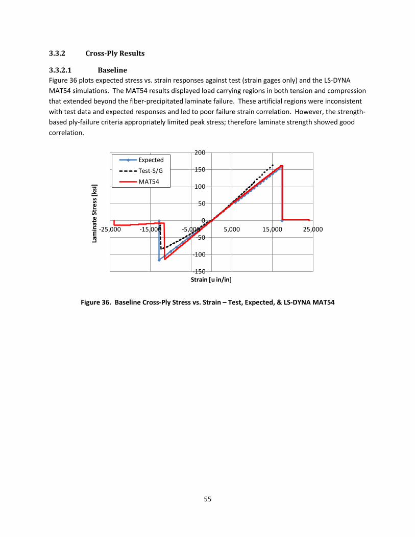
55

3.3.2 Cross-Ply Results

3.3.2.1 Baseline Figure 36 plots expected stress vs. strain responses against test (strain gages only) and the LS-DYNA MAT54 simulations. The MAT54 results displayed load carrying regions in both tension and compression that extended beyond the fiber-precipitated laminate failure. These artificial regions were inconsistent with test data and expected responses and led to poor failure strain correlation. However, the strength-based ply-failure criteria appropriately limited peak stress; therefore laminate strength showed good correlation.

Figure 36. Baseline Cross-Ply Stress vs. Strain – Test, Expected, & LS-DYNA MAT54

-150

-100

-50

0

50

100

150

200

-25,000 -15,000 -5,000 5,000 15,000 25,000

Lam

inat

e St

ress

[ksi

]

Strain [u in/in]

ExpectedTest-S/GMAT54

56

The unusual LS-DYNA response can be understood by recalling the MAT54 ply behavior uncovered in the previous UD simulations; namely that the Chang-Chang strength-based failure-criteria initiated ply degradation, while ply- and element deletion only occurred by the DFAIL failure strains. Figure 37 shows that UD 1-direction (fiber) response was linear-elastic to brittle failure in both tension and compression. Here the fiber strengths and DFAIL failure strains were coincident.

Figure 37. MAT54 Fiber/1-Dir, Matrix/2-Dir, & Average Behavior

In contrast only a single failure strain parameter (DFAILM) was available for the material 2-direction (matrix) response. In the case of the Toray T700GC 12k/2510 material system, this led to artificial elastic-plastic tensile behavior shown in exaggerated scale on Figure 37. The UD study also confirmed that element deletion does not occur until the largest ply failure strain in the loading direction was exceeded.

The experimental results in Figure 36 confirmed that laminate response was the average of the 0º and 90º ply groups. Figure 37 shows the unusual and physically-incorrect MAT54 behavior when ply responses are averaged. The pronounced matrix (90º ply) artificial tensile plastic region remained since the largest failure strain (DFAILM > DFAILT) governed element deletion.

The averaged response also created physically inconsistent behavior in compression. An artificial (albeit low stress) load-carrying region existed past fiber (0º ply) failure since the element was not deleted until the failure strain of all plies was exceeded (|DFAILM| > |DFAILC|)).

ε

σ

XT

DFA

ILT

DFA

ILC

ε2t

DFA

ILM

YT

DFA

ILM

XC

YC

1-dir Fiber

2-dir Matrix

Artificial Plastic Region (Matrix)

Avg.

57

Figure 38 plots tested and expected energy vs. strain against the MAT54 simulations. The extended MAT54 artificial load carrying regions in tension and compression were pronounced in this figure; however, the matrix-dominated zones minimally impacted peak strain errors.

Figure 38. Baseline Cross-Ply Energy vs. Strain – Test, Expected, & LS-DYNA MAT54

Load vs. displacement curves are provided in Figure 39, which show reasonable peak load correlation but poor displacement correlation at failure. Results for the pair of strain gage (S/G) specimens are highlighted in the plot.

Figure 39. Baseline Cross-Ply Load vs. Displacement – Test, Expected, & LS-DYNA MAT54

0

200

400

600

800

1000

1200

1400

1600

-25,000 -15,000 -5,000 5,000 15,000 25,000

Ener

gy [l

bf*i

n]

Strain [u in/in]

ExpectedTest-S/GMAT54

-15000

-10000

-5000

0

5000

10000

15000

20000

-0.15 -0.10 -0.05 0.00 0.05 0.10 0.15 0.20 0.25

Forc

e [lb

f]

Displ. [in]

ExpectedMAT54TestTest-S/G

58

Table 19. Cross-Ply Baseline Results – LS-DYNA MAT54 & Theory

Table 19 lists the error between the LS-DYNA MAT54 simulations and expected values. Tensile and compressive failure strain errors were 38% and 86% respectively. These large errors were evident in Figure 36, Figure 38, and Figure 39 and were caused by the following:

• The sole MAT54 material 2-dir (matrix) failure strain (DFAILM) led to tensile elastic-plastic behavior.

• The largest ply failure strain in the loading direction (DFAILM) determined element deletion, creating an artificial post-fiber (0º ply) failure compressive load-carrying region.

The table indicates good correlation for elastic modulus, strength, and overall energy with errors less than 10%. As witnessed in Figure 38, the large errors in failure strain did not negatively impact energy results because the 90º plies carried minimal load in the plastic region after 0º ply fiber failure, contributing very little energy. Interestingly, compressive modulus yielded the 10% error because MAT54 only allows a single modulus for both tension and compression; the tensile value was selected for the MAT54 simulations.

Loading Quantity Force Modulus Strength Strain Energy[lbf] [Msi] [ksi] [u in/in] [lbf*in]

Tension Expected 15,089 9.81 160 17,337 1,140MAT54 15,417 9.86 163 23,988 1,221Error 2% 0% 2% 38% 7%

Compression Expected -11,291 8.99 -116 -12,909 441MAT54 -11,054 9.86 -114 -23,985 465Error -2% 10% -2% 86% 6%

59

In addition to element-level macroscopic results, integration-point and nodal results were reviewed because laminate and lamina stresses were no longer identical. Figure 40 d-f shows stresses for the 0º (fiber) and 90º plies (matrix). Here on-axis ply behavior (aligned with loading direction) was consistent with the UD simulations; peak ply stresses matched the input strengths (XT, YT, etc.) since the Chang-Chang failure criteria reduced to maximum strength criteria for the simplified loading. Also ply/element deletion was governed by the failure strains (DFAILi), which led to plasticity whenever the failure strain exceeded the Chang-Chang failure strength. Figure 40 e also shows off-axis stresses developing as desired due to modulus mismatch between the 0- and 90-plies.

Figure 40. Baseline Cross-Ply Plots – Laminate and Ply Stresses

-2 -1 0 1 2

x 104

-200

-100

0

100

200

Strain [µin/in]

Stre

ss [k

si]

a) Element Stress vs. Strain

-2 -1 0 1 2

x 104

0

0.5

1

Strain [µin/in]

Ener

gy [l

b f*in]

b) Total Energy

-2 -1 0 1 2

x 104

-1000

0

1000

Strain [µin/in]

Forc

e [lb

f]

c) Reaction Force

-2 -1 0 1 2

x 104

-400

-200

0

200

400

Strain [µin/in]

Stre

ss [k

si]

d) 0° Fiber/1-Dir Ply Stress

-2 -1 0 1 2

x 104

-20

0

20

Strain [µin/in]

Stre

ss [k

si]

f) 90° Matrix/2-Dir Ply Stress

-2 -1 0 1 2

x 104

-20

0

20

Strain [µin/in]

Stre

ss [k

si]

e) Off-Axis Ply Stress

0° Matrix-290° Fiber-1

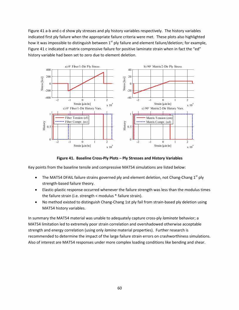
60

Figure 41 a-b and c-d show ply stresses and ply history variables respectively. The history variables indicated first ply failure when the appropriate failure criteria were met. These plots also highlighted how it was impossible to distinguish between 1st ply failure and element failure/deletion; for example, Figure 41 c indicated a matrix compressive failure for positive laminate strain when in fact the “ed” history variable had been set to zero due to element deletion.

Figure 41. Baseline Cross-Ply Plots – Ply Stresses and History Variables

Key points from the baseline tensile and compressive MAT54 simulations are listed below:

• The MAT54 DFAIL failure strains governed ply and element deletion, not Chang-Chang 1st ply strength-based failure theory.

• Elastic-plastic response occurred whenever the failure strength was less than the modulus times the failure strain (i.e. strength < modulus * failure strain).

• No method existed to distinguish Chang-Chang 1st ply fail from strain-based ply deletion using MAT54 history variables.

In summary the MAT54 material was unable to adequately capture cross-ply laminate behavior; a MAT54 limitation led to extremely poor strain correlation and overshadowed otherwise acceptable strength and energy correlation (using only lamina material properties). Further research is recommended to determine the impact of the large failure strain errors on crashworthiness simulations. Also of interest are MAT54 responses under more complex loading conditions like bending and shear.

-2 -1 0 1 2

x 104

-400

-200

0

200

400

Strain [µin/in]

Stre

ss [k

si]

a) 0° Fiber/1-Dir Ply Stress

-2 -1 0 1 2

x 104

-40

-20

0

20

40

Strain [µin/in]

Stre

ss [k

si]

b) 90° Matrix/2-Dir Ply Stress

-2 -1 0 1 2

x 104

0

0.5

1

Strain [µin/in]

Hist

ory

c) 0° Fiber/1-Dir History Vars.

Fiber Tension (ef)Fiber Compr. (ec)

-2 -1 0 1 2

x 104

0

0.5

1

Strain [µin/in]

Hist

ory

c) 90° Matrix/2-Dir History Vars.

Matrix Tension (em)Matrix Compr. (ed)

61

3.3.2.2 Parametric

3.3.2.2.1 Constitutive Parameters

3.3.2.2.1.1 EA Figure 42 shows the result of varying the MAT54 fiber modulus EA. As anticipated, EA significantly impacted the laminate response as it defined the stiffness of plies aligned with the loading. Figure 42 a, b, & c show large changes in laminate stress vs. strain, simulation energy, and 0º ply stress vs. strain respectively; 90º ply stress was not impacted (Figure 42 d).

Figure 42. Cross-Ply Parametric Study – Fiber/1-Dir Modulus (EA) Plots

Figure 42 highlights the dependency of simulation results on the “DFAIL” failure strains independent of the modulus EA. Element deletion was governed by the largest failure strain aligned with the loading direction; in this case, the matrix strain DFAILM (0.024 in/in). Failure strains DFAILT (0.0174 in/in) and DFAILC (0.0128 in/in) also defined the extents of 0º ply load-carrying. These behaviors were evident at both the ply (Figure 42 c-d) and laminate level (Figure 42 a-b).

The artificial load carrying regions witnessed in the baseline simulations were also evident in the EA simulations. In fact, doubling EA to 36.8 Msi created additional tensile and compressive plastic zones (when the 0º plies reached the fiber strengths XT and XC well before the fiber strains DFAILT and DFAILC).

-2 -1 0 1 2

x 104

-100

-50

0

50

100

150

Strain [µin/in]

Stre

ss [k

si]

a) Element Stress vs. Strain

BaselineEA = 1.2EA = 9.2EA = 36.8

-2 -1 0 1 2

x 104

0

0.5

1

1.5

Strain [µin/in]

Ener

gy [l

b f*in]

b) Energy vs. Strain

-2 -1 0 1 2

x 104

-400

-200

0

200

400

Strain [µin/in]

Stre

ss [k

si]

c) 0° Fiber/1-Dir Ply Stress

-2 -1 0 1 2

x 104

-30

-20

-10

0

10

20

30

Strain [µin/in]

Stre

ss [k

si]

d) 90° Matrix/2-Dir Ply Stress

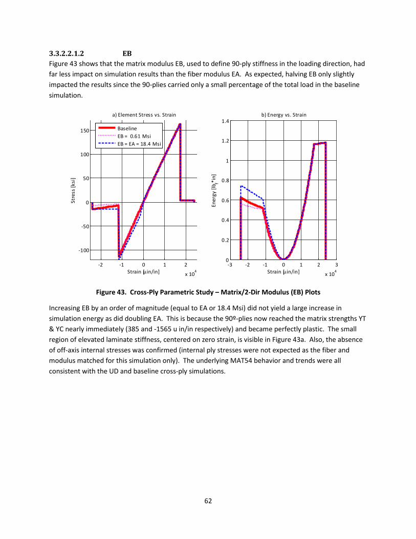
62

3.3.2.2.1.2 EB Figure 43 shows that the matrix modulus EB, used to define 90-ply stiffness in the loading direction, had far less impact on simulation results than the fiber modulus EA. As expected, halving EB only slightly impacted the results since the 90-plies carried only a small percentage of the total load in the baseline simulation.

Figure 43. Cross-Ply Parametric Study – Matrix/2-Dir Modulus (EB) Plots

Increasing EB by an order of magnitude (equal to EA or 18.4 Msi) did not yield a large increase in simulation energy as did doubling EA. This is because the 90º-plies now reached the matrix strengths YT & YC nearly immediately (385 and -1565 u in/in respectively) and became perfectly plastic. The small region of elevated laminate stiffness, centered on zero strain, is visible in Figure 43a. Also, the absence of off-axis internal stresses was confirmed (internal ply stresses were not expected as the fiber and modulus matched for this simulation only). The underlying MAT54 behavior and trends were all consistent with the UD and baseline cross-ply simulations.

-2 -1 0 1 2

x 104

-100

-50

0

50

100

150

Strain [µin/in]

Stre

ss [k

si]

a) Element Stress vs. Strain

BaselineEB = 0.61 MsiEB = EA = 18.4 Msi

-3 -2 -1 0 1 2 3

x 104

0

0.2

0.4

0.6

0.8

1

1.2

1.4

Strain [µin/in]

Ener

gy [l

b f*in]

b) Energy vs. Strain

63

3.3.2.2.2 Strength Parameters The following sections discuss the results of varying the MAT54 strength parameters XT (1-dir/fiber tension), XC (1-dir/fiber compression), YT (2-dir matrix tension), and YC (2-dir matrix compression).

3.3.2.2.2.1 XT As expected, XT greatly affected simulation results because it governed the laminate’s prime load-carrying plies (0º). Figure 44b shows corresponding decrements to the simulation energy when XT was decreased from the baseline 319 ksi under tensile loading. In these cases a pronounced plastic region appeared between the reduced tensile strength and the ply failure strain DFAILT – behavior not physically expected but consistent with behavior uncovered in the MAT54 UD simulations. These large plastic regions were captured in the laminate (Figure 44 a) and 0º ply-stresses (not shown).

Counter intuitively, increasing XT above the baseline value did not increase simulation energy. The DFAILT fiber tensile failure strain governed the 0-ply deletion, which prevented the higher strength XT from being reached.

Figure 44. Cross-Ply Parametric Study – Fiber Tensile Strength (XT) Plots – Tensile Loading

0 0.5 1 1.5 2 2.5

x 104

0

20

40

60

80

100

120

140

160

Strain [µin/in]

Stre

ss [k

si]

a) Element Stress vs. Strain

BaselineXT = 7XT = 160XT = 479

0 0.5 1 1.5 2 2.5

x 104

0

0.2

0.4

0.6

0.8

1

1.2

Strain [µin/in]

Ener

gy [l

b f*in]

b) Energy vs. Strain

64

XT did not meaningfully affect laminate results (stress vs. strain, energy, or reaction force) under compressive loading. However at 2 ksi it was low enough to affect off-axis ply stresses because the 90º plies were under small amounts of tension due to mismatch between ply moduli. Figure 45 showed no perceptible change to laminate stress, but 90º ply matrix off-axis stress was limited to 2 ksi.

Figure 45. Cross-Ply Parametric Study – Fiber Tensile Strength (XT) Plots – Compressive Loading

-2.5 -2 -1.5 -1 -0.5 0

x 104

-120

-100

-80

-60

-40

-20

0

Strain [µin/in]

Stre

ss [k

si]

a) Element Stress vs. Strain

BaselineXT = 2XT = 5

-2.5 -2 -1.5 -1 -0.5 0

x 104

0

0.5

1

1.5

2

2.5

3

3.5

4

4.5

5

Strain [µin/in]

Stre

ss [k

si]

b) 90° Matrix/2-Dir Ply Stress

65

3.3.2.2.2.2 XC The fiber compressive strength parameter XC displayed similar trends as XT except under compressive loading.

Figure 46. Cross-Ply Parametric Study – Fiber Compressive Strength (XC) Plots

Halving XC from 213 to 107 ksi decreased the fiber peak stress as expected. A pronounced plastic region was created and was evident in laminate stress, 0º-ply stress, and energy plots (Figure 46 a, c, b respectively). Increasing XC to 234 ksi did not significantly change the simulation results; once again a failure strain (DFAILC in this case) deleted the ply before higher strength (XC) was reached.

Similar to the case of XT and compressive loading, XC only minimally affected tensile simulations and only if it was set smaller than the minimal off-axis compressive stresses.

-2.5 -2 -1.5 -1 -0.5 0

x 104

-100

0

100

Strain [µin/in]

Stre

ss [k

si]

a) Element Stress vs. Strain

BaselineXC = 107XC = 234

-2.5 -2 -1.5 -1 -0.5 0

x 104

0

0.2

0.4

0.6

0.8

Strain [µin/in]

Ener

gy [l

b f*in]

b) Energy vs. Strain

-2.5 -2 -1.5 -1 -0.5 0

x 104

-250

-200

-150

-100

-50

0

Strain [µin/in]

Stre

ss [k

si]

c) 0° Fiber/1-Dir Ply Stress

-2.5 -2 -1.5 -1 -0.5 0

x 104

-30

-20

-10

0

10

20

30

Strain [µin/in]

Stre

ss [k

si]

d) 90° Matrix/2-Dir Ply Stress

66

3.3.2.2.2.3 YT The MAT54 matrix/2-dir tensile and compressive strengths YT and YC captured the behavior of the 90º plies in the loading direction. As such their impact was expected to be a second order effect since the 90º plies only carried 6% of the total load in the baseline simulation.

Figure 47. Cross-Ply Parametric Study – Matrix Tensile Strength (YT) Plots

Figure 47 a and b show minor increases to the overall laminate stress and energy for tensile loading when YT was increased from 7.09 to 29.3 ksi. The 29.3 ksi value coincided with the failure strain DFAILM; as such this removed the plastic region from the baseline simulation (Figure 47 d). Increasing YT above 29.3 ksi would not further change the results as DFAILM would delete the element first.

Decreasing YT below the baseline to 3 ksi simply limited 90º ply stress lower and lengthened the artificial plastic region. A value of 3 ksi also limited the off-axis ply stresses to 3 ksi, which reached approximately 5 ksi in the baseline simulation.

The YT parameter did not affect results for compressive loading because no matrix tensile loads developed anywhere in the laminate. This was confirmed by reviewing results when YT was reduced to 1 ksi.

0 0.5 1 1.5 2 2.5

x 104

0

50

100

150

Strain [µin/in]

Stre

ss [k

si]

a) Element Stress vs. Strain

BaselineYT = 3YT = 29.3

0 0.5 1 1.5 2 2.5

x 104

0

0.5

1

Strain [µin/in]

Ener

gy [l

b f*in]

b) Energy vs. Strain

0 0.5 1 1.5 2 2.5

x 104

0

100

200

300

Strain [µin/in]

Stre

ss [k

si]

c) 0° Fiber/1-Dir Ply Stress

0 0.5 1 1.5 2 2.5

x 104

0

10

20

30

Strain [µin/in]

Stre

ss [k

si]

d) 90° Matrix/2-Dir Ply Stress

67

3.3.2.2.2.4 YC Figure 48 indicates that the matrix compressive strength YC only had a minor impact on laminate stress and simulation energy for compressive loading. Halving YC from 28.8 to 14.4 ksi created an artificial plastic region in the 90º plies (Figure 48 d); it also changed laminate behavior beyond 0º fiber failure to perfectly plastic. As always, the failure strain parameter DFAILM (24,000 u-in/in) governed element deletion.

Figure 48. Cross-Ply Parametric Study – Matrix Compressive Strength (YC) Plots

The only affect of increasing YC to 31.7 ksi was to eliminate a minute plastic region that occurred in the 90º fibers. This region was caused by DFAILT (0.024 in/in) and the quotient of YT and matrix modulus (EB) being different by rounding error. Increasing YC above 31.7 ksi would not further change the results as DFAILM would delete the ply first.

The YC parameter did not affect the tensile simulations as no matrix compressive loads developed anywhere in the laminate. This was confirmed by reviewing results when YC was reduced to 1 ksi.

-2.5 -2 -1.5 -1 -0.5 0

x 104

-120

-100

-80

-60

-40

-20

0

Strain [µin/in]

Stre

ss [k

si]

a) Element Stress vs. Strain

BaselineYC = 14YC = 32

-2.5 -2 -1.5 -1 -0.5 0

x 104

0

0.1

0.2

0.3

0.4

0.5

0.6

Strain [µin/in]En

ergy

[lb f*i

n]

b) Energy vs. Strain

-2.5 -2 -1.5 -1 -0.5 0

x 104

-250

-200

-150

-100

-50

0

Strain [µin/in]

Stre

ss [k

si]

c) 0° Fiber/1-Dir Ply Stress

-2.5 -2 -1.5 -1 -0.5 0

x 104

-30

-25

-20

-15

-10

-5

0

Strain [µin/in]

Stre

ss [k

si]

d) 90° Matrix/2-Dir Ply Stress

68

3.3.2.2.3 Strain Parameters The MAT54 ply strain parameters DFAILT, DFAILC, and DFAILM solely determined ply and element deletion and were expected to largely influence simulation results.

3.3.2.2.3.1 DFAILT Figure 49 a) and b) depict element stress and energy respectively. As predicted, the fiber/1-dir MAT54 tensile failure strain parameter DFAILT greatly affected simulation results. Halving DFAILT relative to the baseline (0.0174 in/in) limited 0 ply stress by deleting the 0 plies prior to reaching the tensile failure strength XT (319 ksi). As such, the simulation energy was greatly diminished relative to the baseline. However, the element failure strain was unchanged as it was governed by the largest strain parameter in the loading direction – DFAILM in this case for the 90º plies.

In contrast, increasing DFAILT to 0.024 in/in delayed deletion of the 0º plies and significantly increased the simulation energy. Here 0º ply stresses were limited by XT but the resulting large plastic zone added significant energy. The matrix (DFAILM) and fiber tensile (DFAILT) strain parameters were identical for this case only and both determined element failure.

Figure 49. Cross-Ply Parametric Study – Fiber Tensile Strain (DFAILT) Plots

Setting DFAILT (0.025 in/in) larger than DFAILM (0.024 in/in) extended the simulation time, which confirmed that the largest DFAIL strain in the loading direction governed element deletion under simplified loading. Figure 50 indeed showed coincident 0º ply and element failures that extend beyond 0.024 in/in as in the baseline.

Simulations were also run for the same DFAILT parameters subject to compressive loading; results for the compressive simulations were unchanged from the baseline.

0 0.5 1 1.5 2 2.5

x 104

0

50

100

150

200

Strain [µin/in]

Stre

ss [k

si]

a) Element Stress vs. Strain

0 0.5 1 1.5 2 2.5

x 104

0

0.5

1

1.5

2

Strain [µin/in]

Ener

gy [l

b f*in]

b) Energy vs. Strain

BaselineDFAILT = 0.009DFAILT = 0.024DFAILT = 0.025

0 0.5 1 1.5 2 2.5

x 104

0

100

200

300

400

Strain [µin/in]

Stre

ss [k

si]

c) 0° Fiber/1-Dir Ply Stress

0 0.5 1 1.5 2 2.5

x 104

0

5

10

Strain [µin/in]

Stre

ss [k

si]

d) 90° Matrix/2-Dir Ply Stress

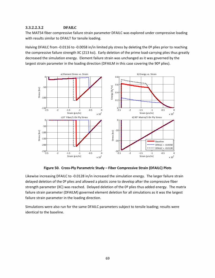
69

3.3.2.2.3.2 DFAILC The MAT54 fiber compressive failure strain parameter DFAILC was explored under compressive loading with results similar to DFAILT for tensile loading.

Halving DFAILC from -0.0116 to -0.0058 in/in limited ply stress by deleting the 0º plies prior to reaching the compressive failure strength XC (213 ksi). Early deletion of the prime load-carrying plies thus greatly decreased the simulation energy. Element failure strain was unchanged as it was governed by the largest strain parameter in the loading direction (DFAILM in this case covering the 90º plies).

Figure 50. Cross-Ply Parametric Study – Fiber Compressive Strain (DFAILC) Plots

Likewise increasing DFAILC to -0.0128 in/in increased the simulation energy. The larger failure strain delayed deletion of the 0º plies and allowed a plastic zone to develop after the compressive fiber strength parameter (XC) was reached. Delayed deletion of the 0º plies thus added energy. The matrix failure strain parameter (DFAILM) governed element deletion for all simulations as it was the largest failure strain parameter in the loading direction.

Simulations were also run for the same DFAILC parameters subject to tensile loading; results were identical to the baseline.

-2.5 -2 -1.5 -1 -0.5 0

x 104

-150

-100

-50

0

Strain [µin/in]

Stre

ss [k

si]

a) Element Stress vs. Strain

-2.5 -2 -1.5 -1 -0.5 0

x 104

0

0.2

0.4

0.6

0.8

Strain [µin/in]En

ergy

[lb f*i

n]

b) Energy vs. Strain

-2.5 -2 -1.5 -1 -0.5 0

x 104

-250

-200

-150

-100

-50

0

Strain [µin/in]

Stre

ss [k

si]

c) 0° Fiber/1-Dir Ply Stress

-2.5 -2 -1.5 -1 -0.5 0

x 104

-30

-20

-10

0

Strain [µin/in]

Stre

ss [k

si]

d) 90° Matrix/2-Dir Ply Stress

BaselineDFAILC = -0.0058DFAILC = -0.0128

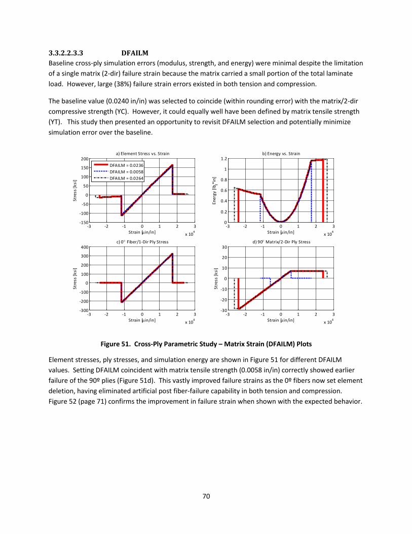
70

3.3.2.2.3.3 DFAILM Baseline cross-ply simulation errors (modulus, strength, and energy) were minimal despite the limitation of a single matrix (2-dir) failure strain because the matrix carried a small portion of the total laminate load. However, large (38%) failure strain errors existed in both tension and compression.

The baseline value (0.0240 in/in) was selected to coincide (within rounding error) with the matrix/2-dir compressive strength (YC). However, it could equally well have been defined by matrix tensile strength (YT). This study then presented an opportunity to revisit DFAILM selection and potentially minimize simulation error over the baseline.

Figure 51. Cross-Ply Parametric Study – Matrix Strain (DFAILM) Plots

Element stresses, ply stresses, and simulation energy are shown in Figure 51 for different DFAILM values. Setting DFAILM coincident with matrix tensile strength (0.0058 in/in) correctly showed earlier failure of the 90º plies (Figure 51d). This vastly improved failure strains as the 0º fibers now set element deletion, having eliminated artificial post fiber-failure capability in both tension and compression. Figure 52 (page 71) confirms the improvement in failure strain when shown with the expected behavior.

-3 -2 -1 0 1 2 3

x 104

-150

-100

-50

0

50

100

150

200

Strain [µin/in]

Stre

ss [k

si]

a) Element Stress vs. Strain

DFAILM = 0.0236DFAILM = 0.0058DFAILM = 0.0264

-3 -2 -1 0 1 2 3

x 104

0

0.2

0.4

0.6

0.8

1

1.2

Strain [µin/in]

Ener

gy [l

b f*in]

b) Energy vs. Strain

-3 -2 -1 0 1 2 3

x 104

-300

-200

-100

0

100

200

300

400

Strain [µin/in]

Stre

ss [k

si]

c) 0° Fiber/1-Dir Ply Stress

-3 -2 -1 0 1 2 3

x 104

-30

-20

-10

0

10

20

30

Strain [µin/in]

Stre

ss [k

si]

d) 90° Matrix/2-Dir Ply Stress

71

Figure 52. Cross-Ply Parametric Study – Matrix Strain (DFAILM) Plots & Theoretical Response

DFAILM was also increased over the baseline with results matching expectations. Figure 51 shows an increase in simulation energy when increasing DFAILM to 0.0264 in/in. The increased DFAILM value simply extends the pre-existing plastic zone in the 90 plies; here DFAILM-based 90 ply and element deletion are identical.

-3 -2 -1 0 1 2 3

x 104

-150

-100

-50

0

50

100

150

200

Strain [µin/in]

Stre

ss [k

si]

a) Element Stress vs. Strain

TheoryDFAILM = YC/EBDFAILM = YT/EB

-3 -2 -1 0 1 2 3

x 104

0

0.2

0.4

0.6

0.8

1

1.2

Strain [µin/in]

Ener

gy [l

b f*in]

b) Energy vs. Strain

72

Table 20 displays strength, failure strain, and energy errors for the DFAILM simulations where DFAILM was set to coincide with the matrix tensile (YT) and compressive (YC) strengths. Results when DFAILM was based on matrix tensile strength nearly eliminated errors in tension (failure strain, strength, and energy) and also drastically improved compressive failure strain. These improvements were credited to elimination of element load-carrying capability beyond 0º fiber failure in both loading directions.

Table 20. Cross-Ply Parametric Study – Matrix Strain (DFAILM) Error Summary

Strength and energy errors slightly increased to -8% and -16% respectively in compression for the YT-based DFAILM simulation. However, the true magnitude of DFAILM-based compressive error was masked by another MAT54 limitation; a single elastic modulus (one each for fiber and matrix) represented both tension and compression.

Quantity Units ExpectedBaseline (YC/EB) YT/EB Expected

Baseline (YC/EB) YT/EB

DFAILM u in/in 17,337 24,000 5,811 12,909 24,000 5,811Strength ksi 159.5 163.0 159.5 -116.0 -113.5 -106.5

Strenth Error - - 2% 0% - -2% -8%Strain u in/in 17,337 23,990 17,390 -12,909 -23,980 -11,590

Strain Error - - 38% 0% - 86% -10%Energy lbf·in 1.10 1.18 1.12 0.59 0.62 0.49

Energy Error - - 7% 1% - 6% -16%

Tension Compression

73

The difference in theoretical (based on AGATE data) and baseline stress vs. strain curves is shown in Figure 53. Use of elastic moduli based on tensile properties exacerbated errors for all compressive simulations as the higher fiber modulus (EA) in LS-DYNA led to smaller fiber failure strains for the same compressive strength (XC or F1cu) This decreased compressive simulation energy for the YT-based DFAILM. In contrast, total energy for the YC-based DFAILM simulation gained energy after fiber failure due to the larger DFAILM (thus over-predicting the simulation energy). Additional simulations were not completed to eliminate elastic moduli based errors from DFAILM-based errors.

Figure 53. Comparison of Theoretical (AGATE-Based) and LS-DYNA Fiber Stress vs. Strain

No single DFAILM value minimized error for all results (strength, failure strain, and energy). Table 20 indicated DFAILM should be based on matrix tensile strength (YT) if accurate element failure strains are a priority; as desired this allowed the stiff 0º fibers to define element failure/deletion in both tension and compression. In contrast, minimum energy and laminate strength errors occurred when basing DFAILM on the matrix failure strength associated with the primary loading direction (either tension or compression).

Recognizing 1) the near elimination of failure strain error, 2) strength and energy errors were of the same order, and 3) compressive energy errors were conservatively under predicted, selecting DFAILM based on matrix tensile strength (YT) offered mildly improved simulation characteristics and error.

-300

-200

-100

0

100

200

300

400

-15,000 -10,000 -5,000 0 5,000 10,000 15,000 20,000

Stre

ss [k

si]

Strain [ksi]

DYNA

Expected

74

3.3.2.3 Summary The LS-DYNA MAT54 material model sufficiently captured the behavior of a simple [0/90]3S cross-ply laminate with the exception of failure strain under idealized uniaxial tensile and compressive loading.

As expected, LS-DYNA laminate stresses were the average of the 0º and 90º plies. Stresses in both ply groups were consistent with trends seen in the UD simulations, showing the undesired plastic regions that occurred when ply strengths were reached before the corresponding DFAIL failure strain. Significant failure strain error could only be eliminated for either tensile or compressive loading since only a single matrix failure strain parameter (DFAILM) existed. The simulations also confirmed the DFAIL-based ply and element deletion.

Strength, energy, and failure strain errors were all less than 16% when redefining the matrix failure strain DFAILM coincident with matrix tensile strength (YT).

Based on the results of this cross-ply MAT54 parametric study, the following enhancements are recommended for the LS-DYNA MAT54 material to improve simulation results without large detriments to computational efficiency:

• Add a matrix/2-dir failure strain to mirror the tensile and compressive values available for the fiber/1-dir.

• Allow tensile and compressive moduli to be defined for both fiber and matrix.

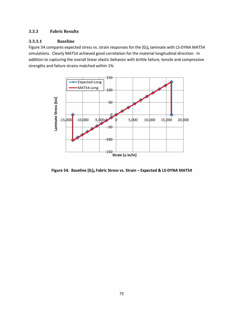
75

3.3.3 Fabric Results

3.3.3.1 Baseline Figure 54 compares expected stress vs. strain responses for the [0f]8 laminate with LS-DYNA MAT54 simulations. Clearly MAT54 achieved good correlation for the material longitudinal direction. In addition to capturing the overall linear elastic behavior with brittle failure, tensile and compressive strengths and failure strains matched within 1%.

Figure 54. Baseline [0f]8 Fabric Stress vs. Strain – Expected & LS-DYNA MAT54

-150

-100

-50

0

50

100

150

-15,000 -10,000 -5,000 0 5,000 10,000 15,000 20,000

Lam

inat

e St

ress

[ksi

]

Strain [u in/in]

Expected-LongMAT54-Long

76

It should be noted that small amounts of plasticity were present in the LS-DYNA results. Figure 55 shows the small plastic region that developed after Chang-Chang ply “fiber” failure (equal to the ply longitudinal strength (XT) for this case). The ply remained fully plastic (limiting ply/laminate stress) until strain-based element deletion (DFAILT). The small plastic region was not unique to this analysis but was present in nearly all simulations when the strength and failure strain were not exactly coincident due to rounding error.

Figure 55. Baseline [0f]8 Fabric Stress vs. Strain – LS-DYNA MAT54 Plasticity

128

129

130

131

132

133

134

16,000 16,100 16,200 16,300 16,400 16,500 16,600

Lam

inat

e St

ress

[ksi

]

Strain [u in/in]

TheoryMAT54

77

Mirroring the good stress vs. strain correlation, Figure 56 shows peak simulation energy matched expected values within 2% after scaling to reflect test specimen geometry (Equations (8)-(11)).

Figure 56. Baseline [0f]8 Fabric Energy vs. Strain – Expected & LS-DYNA MAT54

0

100

200

300

400

500

600

700

800

900

-15,000 -10,000 -5,000 0 5,000 10,000 15,000 20,000

Ener

gy [l

bf*i

n]

Strain [u in/in]

Expected-LongMAT54-Long

78

Figure 57 shows MAT54 history variables for the longitudinal fabric orientation. Tensile and compressive failures were registered by the “ef” and “ec” variables respectively. The variables would have indicated Chang-Chang fiber ply-failure for UD tape; however, in the case of a general orthotropic material, the history variables simply indicated failures along the material longitudinal (1-dir) axis.

Figure 57. Baseline [0f]8 Fabric History Variable vs. Strain – LS-DYNA MAT54

Further examination of Figure 57 shows history variables extending beyond the strength-based ply failures (“ef” and “ec”) to larger strains. This occurred because element (and ply) deletion was governed by the DFAIL failure strains, which slightly exceeded the Chang-Chang failures due to rounding error (also witnessed in Figure 55). Comingled ply and element deletion in the history variables thus removed the ability to distinguish element strain failure mode.

0

0.2

0.4

0.6

0.8

1

1.2

-0.02 -0.01 0 0.01 0.02Strain [in/in]

ef

ec

em

ed

ec ef

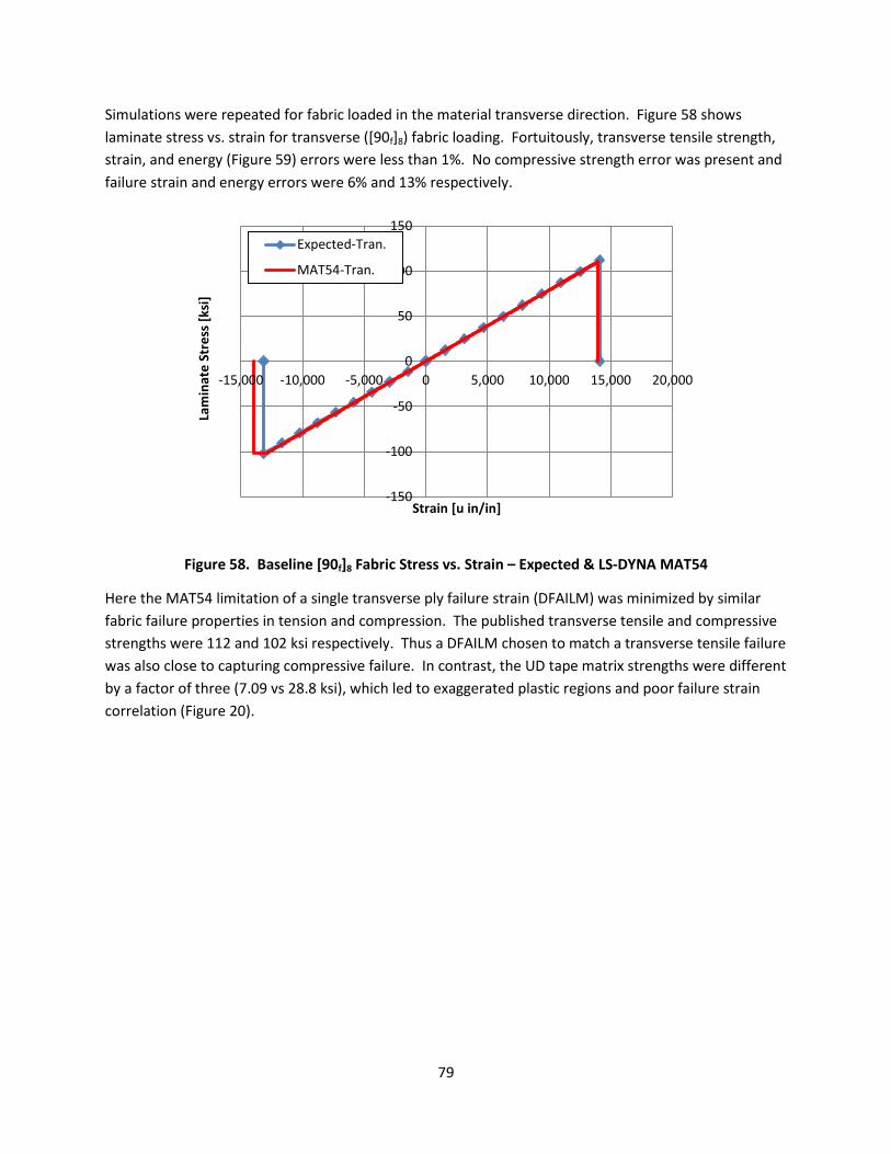
79

Simulations were repeated for fabric loaded in the material transverse direction. Figure 58 shows laminate stress vs. strain for transverse ([90f]8) fabric loading. Fortuitously, transverse tensile strength, strain, and energy (Figure 59) errors were less than 1%. No compressive strength error was present and failure strain and energy errors were 6% and 13% respectively.

Figure 58. Baseline [90f]8 Fabric Stress vs. Strain – Expected & LS-DYNA MAT54

Here the MAT54 limitation of a single transverse ply failure strain (DFAILM) was minimized by similar fabric failure properties in tension and compression. The published transverse tensile and compressive strengths were 112 and 102 ksi respectively. Thus a DFAILM chosen to match a transverse tensile failure was also close to capturing compressive failure. In contrast, the UD tape matrix strengths were different by a factor of three (7.09 vs 28.8 ksi), which led to exaggerated plastic regions and poor failure strain correlation (Figure 20).

-150

-100

-50

0

50

100

150

-15,000 -10,000 -5,000 0 5,000 10,000 15,000 20,000

Lam

inat

e St

ress

[ksi

]

Strain [u in/in]

Expected-Tran.

MAT54-Tran.

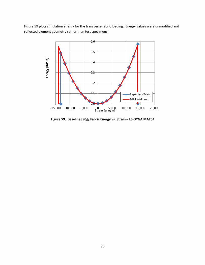
80

Figure 59 plots simulation energy for the transverse fabric loading. Energy values were unmodified and reflected element geometry rather than test specimens.

Figure 59. Baseline [90f]8 Fabric Energy vs. Strain – LS-DYNA MAT54

0.0

0.1

0.2

0.3

0.4

0.5

0.6

-15,000 -10,000 -5,000 0 5,000 10,000 15,000 20,000

Ener

gy [l

bf*i

n]

Strain [u in/in]

Expected-Tran.MAT54-Tran.

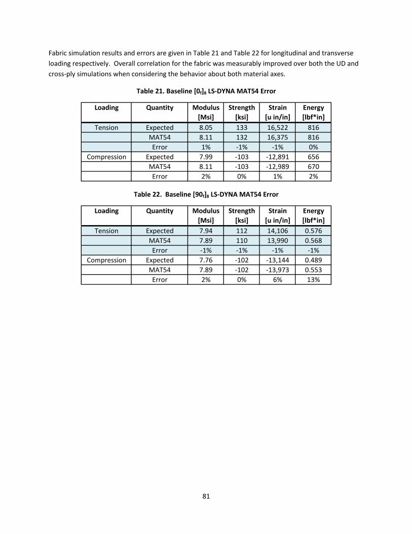
81

Fabric simulation results and errors are given in Table 21 and Table 22 for longitudinal and transverse loading respectively. Overall correlation for the fabric was measurably improved over both the UD and cross-ply simulations when considering the behavior about both material axes.

Table 21. Baseline [0f]8 LS-DYNA MAT54 Error

Table 22. Baseline [90f]8 LS-DYNA MAT54 Error

Loading Quantity Modulus Strength Strain Energy[Msi] [ksi] [u in/in] [lbf*in]

Tension Expected 8.05 133 16,522 816MAT54 8.11 132 16,375 816Error 1% -1% -1% 0%

Compression Expected 7.99 -103 -12,891 656MAT54 8.11 -103 -12,989 670Error 2% 0% 1% 2%

Loading Quantity Modulus Strength Strain Energy[Msi] [ksi] [u in/in] [lbf*in]

Tension Expected 7.94 112 14,106 0.576MAT54 7.89 110 13,990 0.568Error -1% -1% -1% -1%

Compression Expected 7.76 -102 -13,144 0.489MAT54 7.89 -102 -13,973 0.553Error 2% 0% 6% 13%

82

Figure 60 further highlights the improved MAT54 response of the fabric relative to the cross-ply laminate. Figure 60 shows the good MAT54 failure strain correlation of the [0f]8 fabric contrasted with the poor failure strain correlation of the [0/90]3S cross-ply laminate. This result is striking considering the very similar experimental responses of Figure 12.

Figure 60. Stress vs. Strain – Comparison of Baseline Fabric and Cross-Ply

The following are the key points from the baseline MAT54 simulations:

• Overall MAT54 ply behavior was consistent with the previous UD and cross-ply simulations. • Fabric simulations exhibited minimal error about both material axes. This included greatly

improved transverse failure strain correlation over UD and cross-ply simulations, where greater parity between fabric tensile and compressive strengths minimized error from the MAT54 limitation of a single transverse failure strain (DFAILM).

In summary, the MAT54 material model sufficiently captured fabric laminate behavior with only lamina material properties. Further research is recommended to examine mixed-ply orientation lay-ups and more complex loading conditions like bending and shear.

-150

-100

-50

0

50

100

150

200

-30,000 -20,000 -10,000 0 10,000 20,000 30,000

Lam

inat

e St

ress

[ksi

]

Strain [u in/in]

Cross-Ply Expected

Fabric Expected

Cross-Ply MAT54

Fabric MAT54

83

3.3.3.2 Parametric

3.3.3.2.1 Constitutive Parameters

3.3.3.2.1.1 EA – Longitudinal [0f]8

Figure 61 shows the result of varying EA. As expected, a direct correlation existed between ply- and laminate stiffness (modulus) for this single-orientation lay-up with simplified loading. A large plastic zone developed when the modulus was doubled to 16 Msi. The plasticity was initiated after Chang-Chang strength-based ply failure occurred significantly earlier. As in all simulations, this zone extended until element deletion by the tensile or compressive failure strains DFAILT (0.0164 in/in) and DFAILC (0.0130 in/in) respectively.

Figure 61. [0f]8 Fabric Parametric Study – Long. Modulus (EA) Plots

-150

-100

-50

0

50

100

150

-0.02 -0.01 0 0.01 0.02

Stre

ss [k

si]

Strain [in/in]

EA = 4 Msi

EA = 8.11 Msi, baseline

EA = 16 Msi

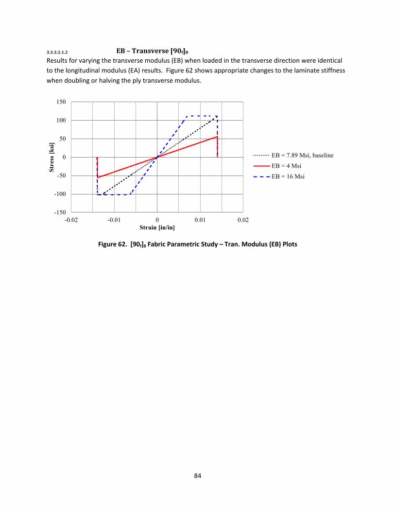
84

3.3.3.2.1.2 EB – Transverse [90f]8

Results for varying the transverse modulus (EB) when loaded in the transverse direction were identical to the longitudinal modulus (EA) results. Figure 62 shows appropriate changes to the laminate stiffness when doubling or halving the ply transverse modulus.

Figure 62. [90f]8 Fabric Parametric Study – Tran. Modulus (EB) Plots

-150

-100

-50

0

50

100

150

-0.02 -0.01 0 0.01 0.02

Stre

ss [k

si]

Strain [in/in]

EB = 7.89 Msi, baseline

EB = 4 Msi

EB = 16 Msi

85

3.3.3.2.2 Strength Parameters

3.3.3.2.2.1 XT Figure 63 shows stress and energy vs. strain for the [0f]8 laminate under tensile loading. Consistent with the UD and cross-ply studies, decreasing XT reduced the maximum ply stress below the baseline and created a plastic region that extended until ply deletion by DFAILT (0.0164 in/in). Interestingly, reducing the strength by 43% to 75 ksi decreased the total energy by only 19% because load carrying capability was maintained throughout plastic region. Counter intuitively from a physical sense, increasing XT above the baseline had no impact on simulation results. The laminate and its plies were deleted at the failure strain DFAILT, which prevented a higher ply or laminate stress from being reached.

Figure 63. [0f]8 Fabric Parametric Study – Long. Tensile Strength (XT) Plots

0

25

50

75

100

125

150

0 0.005 0.01 0.015 0.02

Stre

ss [k

si]

Strain [in/in]

XT = 132 ksi, baseline

XT = 75 ksi

XT = 320 ksi

0

0.01

0.02

0.03

0.04

0.05

0.06

0.07

0.08

0.09

0.1

0 0.005 0.01 0.015 0.02En

ergy

[J]

Strain [in/in]

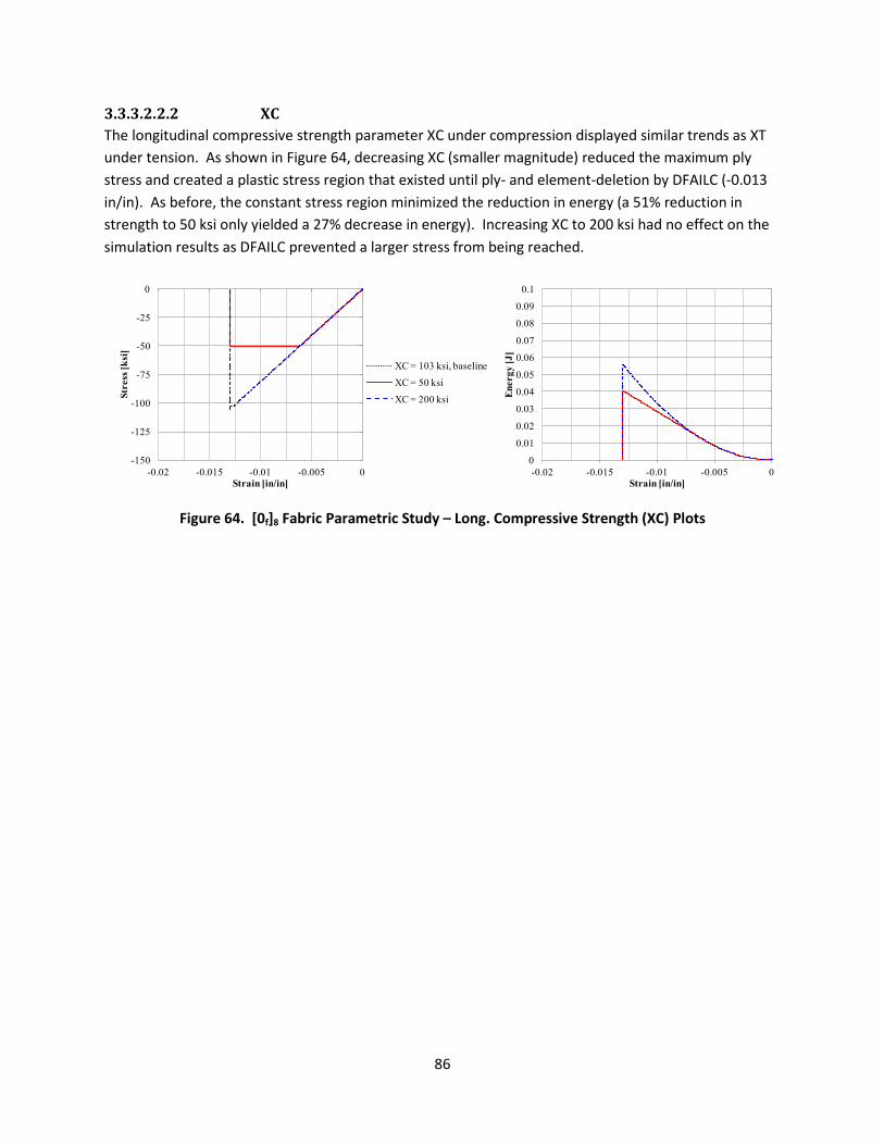
86

3.3.3.2.2.2 XC The longitudinal compressive strength parameter XC under compression displayed similar trends as XT under tension. As shown in Figure 64, decreasing XC (smaller magnitude) reduced the maximum ply stress and created a plastic stress region that existed until ply- and element-deletion by DFAILC (-0.013 in/in). As before, the constant stress region minimized the reduction in energy (a 51% reduction in strength to 50 ksi only yielded a 27% decrease in energy). Increasing XC to 200 ksi had no effect on the simulation results as DFAILC prevented a larger stress from being reached.

Figure 64. [0f]8 Fabric Parametric Study – Long. Compressive Strength (XC) Plots

0

0.01

0.02

0.03

0.04

0.05

0.06

0.07

0.08

0.09

0.1

-0.02 -0.015 -0.01 -0.005 0

Ener

gy [J

]

Strain [in/in]

-150

-125

-100

-75

-50

-25

0

-0.02 -0.015 -0.01 -0.005 0

Stre

ss [k

si]

Strain [in/in]

XC = 103 ksi, baseline

XC = 50 ksi

XC = 200 ksi

87

3.3.3.2.3 Strain Parameters

3.3.3.2.3.1 DFAILT Element tensile stress and simulation energy are shown in Figure 65 for the [0f]8 laminate. As expected, varying DFAILT changed the failure strain in tension. In all cases the plies and element were deleted at DFAILT.

Figure 65. [0f]8 Fabric Parametric Study – Long. Tensile Failure Strain (DFAILT) Plots

DFAILT thus significantly impacted simulation energy. Decreasing DFAILT by 71% to 0.005 in/in led to a 91% decrease in simulation energy. Increasing DFAILT by 46% to 0.024 in/in increased energy by 93%; however, the increase would have been substantially larger if not for the plastic region initiated by the ply strength parameter XT (132 ksi).

3.3.3.2.3.2 DFAILC Similar to DFAILT in the tensile simulations, DFAILC had the ability to significantly impact compressive simulations. Figure 66 shows an 85% decrease in energy when DFAILC was reduced by 61% to -0.005 in/in. Increasing DFAILC beyond the baseline created a plastic stress region that extended from the longitudinal compressive strength XC until element deletion at DFAILC. The constant stress region minimized the energy increase that otherwise would have followed a parabolic trajectory.

Figure 66. [0f]8 Fabric Parametric Study – Long. Compressive Failure Strain (DFAILC) Plots

0

25

50

75

100

125

150

0 0.005 0.01 0.015 0.02 0.025 0.03

Stre

ss [k

si]

Strain [in/in]

DFAILT = 0.0164 in/in, baselineDFAILT = 0.005 in/in

DFAILT = 0.024 in/in

0

0.02

0.04

0.06

0.08

0.1

0.12

0.14

0.16

0.18

0.2

0 0.005 0.01 0.015 0.02 0.025 0.03

Stre

ss [k

si]

Strain [in/in]

-150

-125

-100

-75

-50

-25

0

-0.03 -0.025 -0.02 -0.015 -0.01 -0.005 0

Stre

ss [k

si]

Strain [in/in]

DFAILC = -0.013 in/in, baselineDFAILC = -0.005 in/in

DFAILC = -0.024 in/in

0

0.025

0.05

0.075

0.1

0.125

0.15

0.175

0.2

-0.03 -0.025 -0.02 -0.015 -0.01 -0.005 0

Ener

gy [J

]

Strain [in/in]

88

3.3.3.2.3.3 DFAILM The DFAILM strain parameter governed transverse (material 2-direction) failure in both tension and compression. Unlike the UD and cross-ply simulations, the baseline fabric section concluded that the limitations of a single strain parameter were minimized due to similar fabric transverse properties in tension and compression.

The baseline fabric DFAILM (0.014 in/in) was selected to coincide with the transverse tensile strength (YT). However, it could equally well have been defined by the compressive strength (YC). The DFAILM selection was re-examined to potentially minimize simulation error over the baseline. Figure 67 shows stress and energy versus strain for fabric transverse loading. Clearly, DFAILM selection represented a compromise since both values of DFAILM, one based on YT and the other on YC, caused some error.

Figure 67. [90f]8 Fabric Parametric Study – Transverse Failure Strain (DFAILM) Plots

The trade-off in selecting DFAILM when the published transverse tensile failure strain (e2t) exceeds the compressive (e2c) is exaggerated in Figure 68

Figure 68. Comparison of Expected and MAT54 Transverse Behavior

-150

-100

-50

0

50

100

150

-15,000 -10,000 -5,000 0 5,000 10,000 15,000

Lam

inat

e St

ress

[ksi

]

Strain [u in/in]

Expected-Tran.DFAILM = 0.014 in/inDFAILM = 0.0129 in/in 0.0

0.1

0.2

0.3

0.4

0.5

0.6

-15,000 -10,000 -5,000 0 5,000 10,000 15,000

Ener

gy [l

bf*i

n]

Strain [u in/in]

ε

σ

-YC

YT

e2t

e2c

|e2t| > e2c

Tested Response

-YCEB

Addl.Capability

DFA

ILM

=YT EB

ε

σ

-YC

YT

DFA

ILM

DFAILM = YT/EB

LostCapability

DFAILM = YC/EB

ε

σ

-YC

YT

YC

DFA

ILM

=YC EB

DFA

ILM

89

Table 23 presents transverse simulation errors assuming linear elasticity and brittle failure. Tensile errors (strength, strain, & energy) were obviously minimal when DFAILM was based on the tensile strength YT; likewise, compressive errors were small when DFAILM was YC based. The tension-based DFAILM value was selected for the baseline because it offered lower overall strength, strain, and energy errors when considering both tension and compression.

Table 23. Fabric Parametric Study – Transverse Strain (DFAILM) Error Summary

Figure 69 shows stress and energy versus strain when more exaggerated values of DFAILM were simulated. Decreasing DFAILM by 64% to 0.005 in/in truncated the stress versus strain curve and led to an 87% decrease in simulation energy. Increasing DFAILM by 71% to 0.024 in/in created a plastic region, resulting in a 139% increase in energy.

Figure 69. [90f]8 Fabric Parametric Study – Transverse Failure Strain (DFAILM) Plots

Quantity Units ExpectedBaseline (YT/EB)

YC/EB ExpectedBaseline (YT/EB)

YC/EB

DFAILM u in/in - 14,000 12,900 - 14,000 12,900Strength ksi 112.0 110.4 101.7 -102.0 -102.0 -101.8

Error - -1% -9% - 0% 0%Strain u in/in 14,106 13,990 12,884 -13,144 -13,973 -12,898

Error - -1% -9% 0% 6% -2%Energy J 0.065 0.064 0.054 0.055 0.062 0.054

Error - -1% -16% 0% 13% -3%

Tension Compression

-150

-100

-50

0

50

100

150

-0.03 -0.02 -0.01 0 0.01 0.02 0.03

Stre

ss [k

si]

Strain [in/in]

DFAILM = 0.014 in/in, baselineDFAILM = 0.005 in/in

DFAILM = 0.024 in/in

0

0.025

0.05

0.075

0.1

0.125

0.15

0.175

0.2

-0.03 -0.02 -0.01 0 0.01 0.02 0.03

Ener

gy [J

]

Strain [in/in]

90

3.3.3.3 Summary The LS-DYNA MAT54 material model successfully captured the behavior of a simple [0f]8 fabric laminate under idealized uniaxial tensile and compressive loading about both material axes. The AGATE fabric material system had similar properties in tension and compression, which mitigated a key MAT54 limitation of only having a single transverse failure strain. The similar fabric tensile and compressive properties led to markedly better correlation than the UD and cross-ply simulations (strength, strain, and energy errors were 13% or less) where properties varied greatly depending on the orientation.

General observations from the fabric simulations are summarized below:

• Fabric simulation trends were consistent with UD (tape) simulations except with different material properties.

• Ply and element stress were identical for the simplified lay-up (single ply orientation) and loading (i.e. no bending).

• Rather than highlighting failure of the ply constituents (either matrix or fiber) for UD tape plies, the MAT54 history variables only described failure about a material axis for the fabric material system.

• Changing the MAT54 strengths and failure strains affected simulation results. The strengths effectively set maximum ply stress while the strains governed ply and element deletion. Plastic regions developed when ply strength (in the loading direction) was less than the corresponding failure strain.

• MAT54 DFAIL failure strains were the critical parameters that significantly influenced the results.

The following are recommended to minimize simulation error when modeling fabric:

1. Calculate longitudinal tensile failure strain assuming brittle failure (i.e. DFAILT = XT/EA). 2. Calculate longitudinal compressive failure strain assuming brittle failure (i.e. DFAILC = XC/EA). 3. Examine simulation results for the transverse failure strain DFAILM based on both tensile (YT)

and compressive (YC) strengths; select the transverse failure strain that minimizes simulation errors.

Finally, the same enhancements are recommended for the LS-DYNA MAT54 material model as in the previous sections: namely adding a second transverse failure strain parameter (in addition to DFAILM) and allowing tensile & compressive moduli to be defined for both fiber and matrix. These enhancements do not measurably increase material model complexity from a user standpoint, nor are they expected to detrimentally impact computational efficiency.

91

4. Research Summary and Conclusions Past crashworthiness research at the University of Washington indicated that the LS-DYNA MAT54 material model was behaving contrary to both LS-DYNA documentation and expectations for brittle laminates. Unfortunately, the underlying MAT54 behavior was difficult to isolate in the complex dynamic component-level simulations.

Therefore this research was completed to understand the gamut of MAT54 material model behavior – constitutive relations, ply failure (damage onset), ply deletion, damage factors, element deletion, and parameter influence. MAT54 behavior was isolated by returning to the lowest level of simulation complexity; in particular, a single shell element was loaded under uniaxial tension and compression. The study spanned three idealized laminates amongst two different material systems.

The expected behavior was established from published material properties and additional experimental testing at the University of Washington. Baseline simulation results for UD, cross-ply, and fabric laminates were then compared against the expected results. Once the baseline comparisons were completed, a parametric study was completed for the MAT54 inputs to understand their impacts on simulation results.

UD results most notably characterized MAT54 ply stress strain behavior. The strength-based Chang-Chang ply failure criteria were shown to set maximum ply stresses but did not delete the ply. Instead the ply deletion parameters, typically the DFAIL failure strains, were necessary to end ply load carrying capability. Plastic regions often occurred as a result when the Chang-Chang failure strengths were reached prior to the DFAIL failure strains. The plastic region was prominent for matrix tension, which yielded poor strain and energy correlation and marred otherwise adequate correlation about the remaining material axes and load orientations. The pronounced plastic region was attributed to the single DFAILM failure strain modeling both tensile and compressive matrix failures.

The cross-ply laminate was similarly hampered by poor failure strain correlation. Here the largest ply failure strain in the loading direction (DFAILM) determined element deletion, creating artificial post-fiber failure load-carrying regions. Laminate strength and energy correlation was otherwise acceptable since fiber dominance masked matrix force and energy errors.

The fabric laminate showed good overall correlation for both orientations and load directions. Strength and energy errors were minimal for the fiber-dominated laminate and similar fabric tensile and compressive strengths also nearly eliminated strain errors from the DFAILM limitation.

92

The research found that the DFAIL failure strain parameters should always be entered to ensure ply-deletion and thereby limit excessive ply strains. The DFAIL failure strains should be set consistent with the ply failure strengths where possible to prevent plastic ply response. The response of UD laminates under transverse loading should be examined to optimally select DFAILM and minimize simulation error.

Proposed enhancements to the MAT54 material model and documentation included adding a second DFAIL matrix/transverse failure strain, adding a second elastic modulus about each material axis, separating strength-based ply failure from element deletion in the Chang-Chang failure history variables, and modifying LS-DYNA documentation to emphasize the above ply stress-strain behavior. Further research with quasi-isotropic laminates under more complex bending and shear loading was also recommended.

93

5. Bibliography

[1] J. Carruthers, A. Kettle and A. Robinson, "Energy Absorption Capability and Crashworthiness of Composite Material Structures: A Review," vol. 51, pp. 635-649, 1998.

[2] D. Hull, "A Unified Approach to Progressive Crushing of Fibre-Reinforced Composite Tubes," vol. 40, pp. 377-421, 1991.

[3] P. Soden, A. Kaddour and M. Hinton, "Recommendations For Designers and Researchers Resulting from The World-Wide Failure Exercise," vol. 64, pp. 589-604, 2004.

[4] Department of Defense, Composite Materials Handbook (CMH-17), vol. 2. Polymer Matrix Composites Materials Properties, 2002.

[5] A. Matzenmiller and K. Schweizerhof, Crashworthiness Simulations Of Composite Structures- A First Step With Explicit Time Integration, P. Wriggers and W. Wagner, Eds., Nonlinear Computational Mechanics - A State Of The Art, 1991.

[6] A. Johnson and A. Pickett, "Impact And Crash Modeling Of Composite Structures: A Challenge For Damage Mechanics," in European Conference On Computational Mechanics, Munich, 1999.

[7] J. Wiggenraad, "Crashworthiness Research at NLR," NLR, 2003.

[8] A. Pickett, T. Pyttel, F. Payen, F. Lauro, N. Petrinic, H. Werner and J. Christlein, "Failure Prediction For Advanced Crashworthiness Of Transportation Vehicles," vol. 30, pp. 853-872, 2004.

[9] A. Byar, "A Crashworthiness Study Of A Boeing 737 Fuselage Section," Philadelphia, 2003.

[10] P. Feraboli, F. Deleo, B. Wade, M. Rassaian, M. Higgins, A. Byar, M. Reggiani, A. Bonfatti, L. Deoto and A. Masini, "Predictive Modeling Of An Energy-Absorbing Sandwich Structural Concept Using The Building Block Approach," vol. 41, pp. 774-786, 2010.

[11] J. Gabrys, J. Schatz, K. Carney, M. Melis, E. Fasanella and K. Lyle, "The Use of LS-DYNA in The Columbia Accident Investigation and Return To Flight Activities," in Proceedings Of The 8th International Ls-Dyna Users Conference, Detroit, 2004.

[12] Livermore Software Technology Corporation (LSTC), LS-DYNA Keyword User's Manual, vol. I, Livermore, CA, 2007.

[13] J. Tomblin, J. Sherraden, W. Seneviratne and K. S. Raju, A-Basis and B-Basis Design Allowables for Epoxy – Based Prepreg TORAY T700GC-12K-31E/#2510 Unidirectional Tape [US Units], Wichita, KS:

94

National Institute for Aviation Research, 2002.

[14] J. Tomblin, J. Sherraden, W. Seneviratne and K. S. Raju, A-Basis and B-Basis Design Allowables for Epoxy - Based Prepreg TORAY T700SC-12K-50C/#2510 Plain Weave Fabric [US Units], Wichita, KS: National Institute for Aviation Research, 2010.

[15] ASTM International, Standard Test Method for Tensile Properties of Polymer Matrix Composite Materials (ASTM D 3039-95), West Conshohocken, PA, 2008.

[16] ASTM International, Standard Test Method for Open-Hole Compressive Strength of Polymer Matrix Composite Laminates (ASTM D 6484-09), PA, 2009.

[17] F. Chang and K. Chang, "A Progressive Damage Model For Laminated Composites Containing Stress Concentrations," vol. 21, pp. 834-855, 1987.

[18] Z. Hashin, "Failure Criteria For Unidirectional Fiber Composites," vol. 47, pp. 329-334, 1980.

[19] R. Courant, K. Friedrichs and H. Lewy, "Über De Partiellen Differentialgleichungen Dre Mathematischen Physik," vol. 100, pp. 32-74, 1928.

95

Appendix A. MAT54 Input Parameter Definitions

Variable Definition Suggested Value

MID Material identification number Any arbitrary integer

RO Mass per unit volume* ρ from material properties*

EA Young’s modulus in longitudinal direction. E1, from material properties (tension used)

EB Young’s modulus in transverse direction. E2, from material properties (tension used)

EC Young’s modulus through the thickness Not used

PRBA Minor Poisson’s ratio, vba = v21 Calculated using v12 , E1 and E2

PRCA Minor Poisson's ratio, vca = v31 Not used

PRCB Minor Poisson's ratio, vcb = v32 Not used

GAB Shear modulus, Gab G12, from material properties

GBC Shear modulus, Gbc Assumed equal to Gab

GCA Shear modulus, Gca Assumed equal to Gab

KF Bulk modulus of material Not used

AOPT Material axes option parameter AOPT = 0

XP YP ZP Material axes coordinates for AOPT = 1 Not used

A1 A2 A3

D1 D2 D3 Material axes coordinates for AOPT = 2 Not used

MANGLE Material angle in degrees used when AOPT = 3 Not used

V1 V2 V3 Material axes coordinates for AOPT = 3 Not used

DFAILT Max strain for fiber tension DFAILT = (F1tu / E1) [DFAILT > 0]

DFAILC Max strain for fiber compression DFAILC = (F1cu / E1) [DFAILC < 0]

DFAILM Max strain for matrix straining in tension and compression

DFAILM ≥ max[(YT/EB) , (YC/EB)]

DFAILS Max shear strain 0 < DFAILS ≤ 0.1

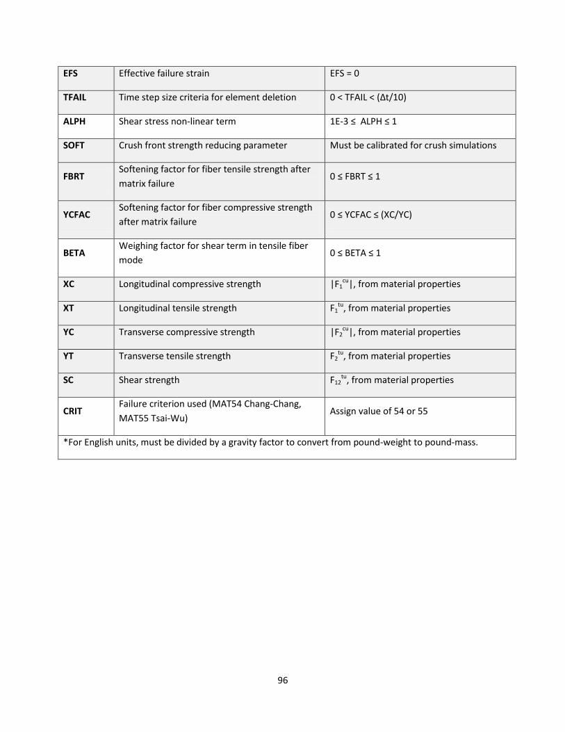
96

EFS Effective failure strain EFS = 0

TFAIL Time step size criteria for element deletion 0 < TFAIL < (Δt/10)

ALPH Shear stress non-linear term 1E-3 ≤ ALPH ≤ 1

SOFT Crush front strength reducing parameter Must be calibrated for crush simulations

FBRT Softening factor for fiber tensile strength after matrix failure

0 ≤ FBRT ≤ 1

YCFAC Softening factor for fiber compressive strength after matrix failure

0 ≤ YCFAC ≤ (XC/YC)

BETA Weighing factor for shear term in tensile fiber mode

0 ≤ BETA ≤ 1

XC Longitudinal compressive strength |F1cu|, from material properties

XT Longitudinal tensile strength F1tu, from material properties

YC Transverse compressive strength |F2cu|, from material properties

YT Transverse tensile strength F2tu, from material properties

SC Shear strength F12tu, from material properties

CRIT Failure criterion used (MAT54 Chang-Chang, MAT55 Tsai-Wu)

Assign value of 54 or 55

*For English units, must be divided by a gravity factor to convert from pound-weight to pound-mass.

97

Appendix B. Baseline LS-DYNA Input Decks

B1. UD [0]12 Tension

$------------------------------------------------------------------------------- $ LS-DYNA(971) DECK $ $ ENGINEER: Bonnie Wade $ ENGINEER: Morgan Osborne $ PROJECT: UW-Lamborghini $ DATE: February 08, 2012 $ UNITS: IN, LB*S*S/IN, SEC, LB $ $------------------------------------------------------------------------------- $ SINGLE-ELEMENT CHARACTERIZATION OF LS-DYNA MAT_054 MATERIAL MODEL $------------------------------------------------------------------------------- *KEYWORD $ $------------------------------------------------------------------------------- $ 1. SOLUTION CONTROL AND OUTPUT PARAMETERS $------------------------------------------------------------------------------- *TITLE Fiber Tension - Run 001 - Baseline $ $ Solution -------------------------------------------------------------------- *CONTROL_TERMINATION $---+----1----+----2----+----3----+----4----+----5----+----6----+----7----+----8 $ ENDTIM ENDCYC DTMIN ENDENG ENDMAS 0.001 0 0.0 0.0 0.0 *CONTROL_TIMESTEP $ DTINIT TSSFAC ISDO TSLIMT DT2MS LCTM ERODE MSIST 0.0 0.5 *CONTROL_SHELL $ WRPANG ESORT IRNXX ISTUPD THEORY BWC MITER PROJ 0.0 0 -1 0 2 2 1 0 $ ROTASCL INTGRD LAMSHT CSTYP6 TSHELL NFAIL1 NFAIL4 PSNFAIL 0.0 1 1 1 0 0 0 *CONTROL_ENERGY $ HGEN RWEN SLNTEN RYLEN 2 2 *CONTROL_ACCURACY $ OSU INN PIDOSU 2 $ $ Database --------------------------------------------------------------------- $ Control ASCII printing intervals $ ELOUT = Element data $ NODFOR = Nodal force groups $ GCEOUT = Geometric contact entities $ RCFORC = Resultant interface forces $ MATSUM = Material energies $ SPCFORC = SPC reaction forces $ SSSTAT = Subsystem data (mass/energy/momentum) $ *DATABASE_ELOUT 1.0000E-05 0 *DATABASE_GCEOUT 1.0000E-05 0 *DATABASE_GLSTAT 1.0000E-05 0 *DATABASE_MATSUM 1.0000E-05 0 *DATABASE_NODFOR 1.0000E-05 0 *DATABASE_RCFORC 1.0000E-05 0 *DATABASE_SPCFORC 1.0000E-06 0 $ $ Binary result intervals *DATABASE_BINARY_D3PLOT $ DT/CYCL LCDT BEAM NPLTC

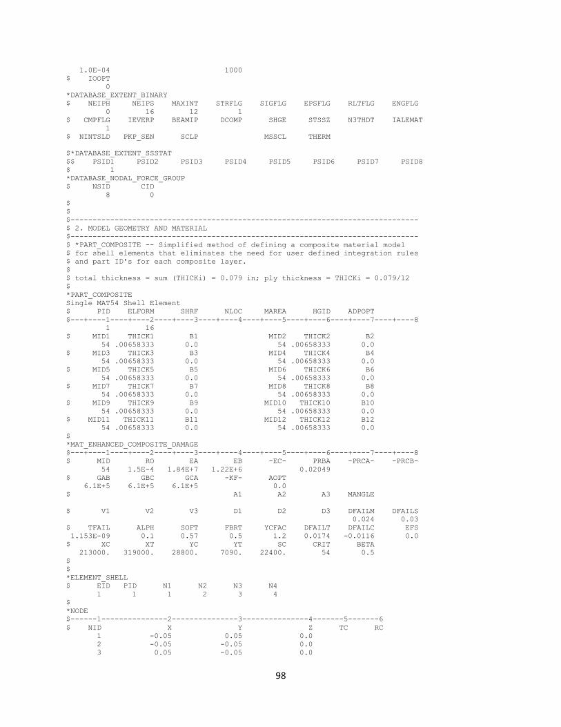
98

1.0E-04 1000 $ IOOPT 0 *DATABASE_EXTENT_BINARY $ NEIPH NEIPS MAXINT STRFLG SIGFLG EPSFLG RLTFLG ENGFLG 0 16 12 1 $ CMPFLG IEVERP BEAMIP DCOMP SHGE STSSZ N3THDT IALEMAT 1 $ NINTSLD PKP_SEN SCLP MSSCL THERM $*DATABASE_EXTENT_SSSTAT $$ PSID1 PSID2 PSID3 PSID4 PSID5 PSID6 PSID7 PSID8 $ 1 *DATABASE_NODAL_FORCE_GROUP $ NSID CID 8 0 $ $ $------------------------------------------------------------------------------- $ 2. MODEL GEOMETRY AND MATERIAL $------------------------------------------------------------------------------- $ *PART_COMPOSITE -- Simplified method of defining a composite material model $ for shell elements that eliminates the need for user defined integration rules $ and part ID's for each composite layer. $ $ total thickness = sum (THICKi) = 0.079 in; ply thickness = THICKi = 0.079/12 $ *PART_COMPOSITE Single MAT54 Shell Element $ PID ELFORM SHRF NLOC MAREA HGID ADPOPT $---+----1----+----2----+----3----+----4----+----5----+----6----+----7----+----8 1 16 $ MID1 THICK1 B1 MID2 THICK2 B2 54 .00658333 0.0 54 .00658333 0.0 $ MID3 THICK3 B3 MID4 THICK4 B4 54 .00658333 0.0 54 .00658333 0.0 $ MID5 THICK5 B5 MID6 THICK6 B6 54 .00658333 0.0 54 .00658333 0.0 $ MID7 THICK7 B7 MID8 THICK8 B8 54 .00658333 0.0 54 .00658333 0.0 $ MID9 THICK9 B9 MID10 THICK10 B10 54 .00658333 0.0 54 .00658333 0.0 $ MID11 THICK11 B11 MID12 THICK12 B12 54 .00658333 0.0 54 .00658333 0.0 $ *MAT_ENHANCED_COMPOSITE_DAMAGE $---+----1----+----2----+----3----+----4----+----5----+----6----+----7----+----8 $ MID RO EA EB -EC- PRBA -PRCA- -PRCB- 54 1.5E-4 1.84E+7 1.22E+6 0.02049 $ GAB GBC GCA -KF- AOPT 6.1E+5 6.1E+5 6.1E+5 0.0 $ A1 A2 A3 MANGLE $ V1 V2 V3 D1 D2 D3 DFAILM DFAILS 0.024 0.03 $ TFAIL ALPH SOFT FBRT YCFAC DFAILT DFAILC EFS 1.153E-09 0.1 0.57 0.5 1.2 0.0174 -0.0116 0.0 $ XC XT YC YT SC CRIT BETA 213000. 319000. 28800. 7090. 22400. 54 0.5 $ $ *ELEMENT_SHELL $ EID PID N1 N2 N3 N4 1 1 1 2 3 4 $ *NODE $------1---------------2---------------3---------------4-------5-------6 $ NID X Y Z TC RC 1 -0.05 0.05 0.0 2 -0.05 -0.05 0.0 3 0.05 -0.05 0.0

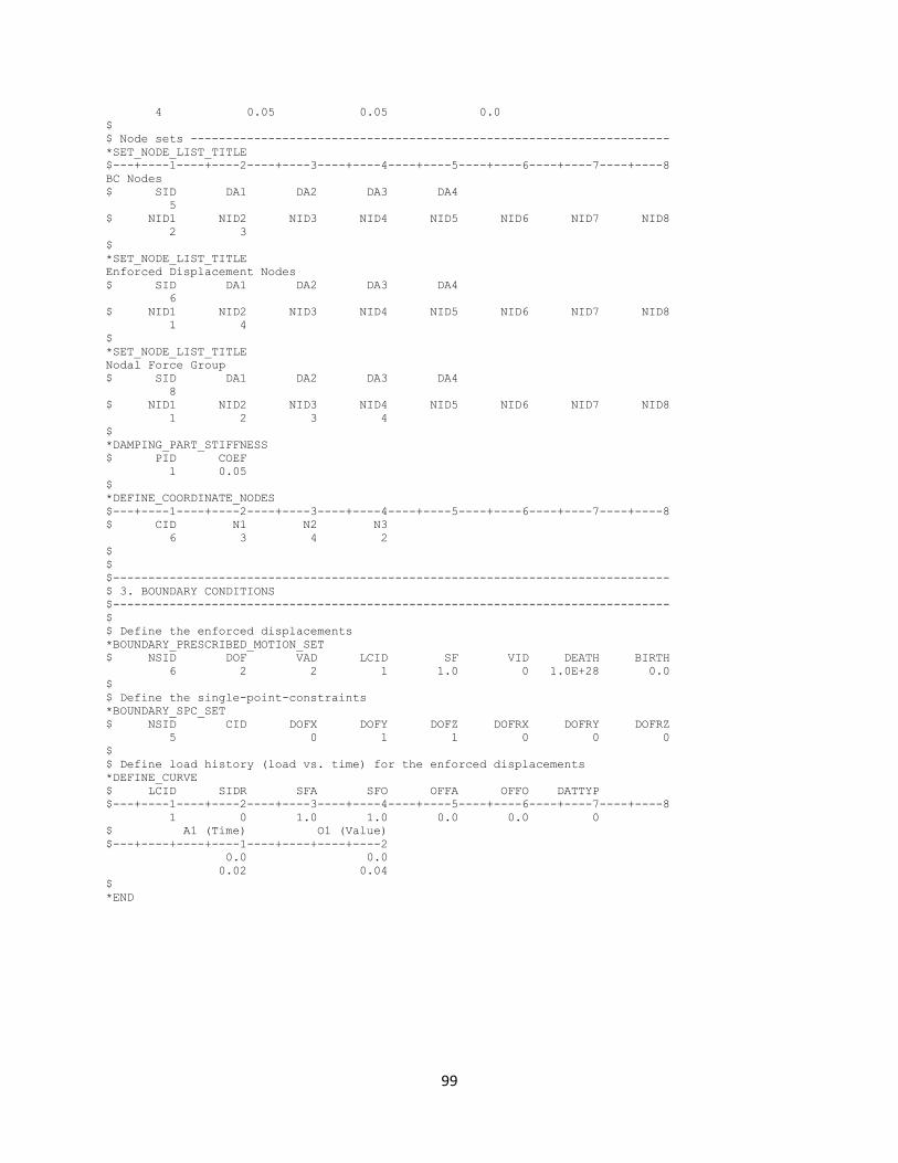
99

4 0.05 0.05 0.0 $ $ Node sets -------------------------------------------------------------------- *SET_NODE_LIST_TITLE $---+----1----+----2----+----3----+----4----+----5----+----6----+----7----+----8 BC Nodes $ SID DA1 DA2 DA3 DA4 5 $ NID1 NID2 NID3 NID4 NID5 NID6 NID7 NID8 2 3 $ *SET_NODE_LIST_TITLE Enforced Displacement Nodes $ SID DA1 DA2 DA3 DA4 6 $ NID1 NID2 NID3 NID4 NID5 NID6 NID7 NID8 1 4 $ *SET_NODE_LIST_TITLE Nodal Force Group $ SID DA1 DA2 DA3 DA4 8 $ NID1 NID2 NID3 NID4 NID5 NID6 NID7 NID8 1 2 3 4 $ *DAMPING_PART_STIFFNESS $ PID COEF 1 0.05 $ *DEFINE_COORDINATE_NODES $---+----1----+----2----+----3----+----4----+----5----+----6----+----7----+----8 $ CID N1 N2 N3 6 3 4 2 $ $ $------------------------------------------------------------------------------- $ 3. BOUNDARY CONDITIONS $------------------------------------------------------------------------------- $ $ Define the enforced displacements *BOUNDARY_PRESCRIBED_MOTION_SET $ NSID DOF VAD LCID SF VID DEATH BIRTH 6 2 2 1 1.0 0 1.0E+28 0.0 $ $ Define the single-point-constraints *BOUNDARY_SPC_SET $ NSID CID DOFX DOFY DOFZ DOFRX DOFRY DOFRZ 5 0 1 1 0 0 0 $ $ Define load history (load vs. time) for the enforced displacements *DEFINE_CURVE $ LCID SIDR SFA SFO OFFA OFFO DATTYP $---+----1----+----2----+----3----+----4----+----5----+----6----+----7----+----8 1 0 1.0 1.0 0.0 0.0 0 $ A1 (Time) O1 (Value) $---+----+----+----1----+----+----+----2 0.0 0.0 0.02 0.04 $ *END

100

B2. Cross-Ply [0/90]3S Tension

$------------------------------------------------------------------------------- $ LS-DYNA(971) DECK $ $ ENGINEER: Bonnie Wade $ ENGINEER: Morgan Osborne $ PROJECT: UW-Lamborghini $ DATE: March 07, 2012 $ UNITS: IN, LB*S*S/IN, SEC, LB $ $------------------------------------------------------------------------------- $ SINGLE-ELEMENT CHARACTERIZATION OF LS-DYNA MAT_054 MATERIAL MODEL $------------------------------------------------------------------------------- *KEYWORD $ $------------------------------------------------------------------------------- $ 1. SOLUTION CONTROL AND OUTPUT PARAMETERS $------------------------------------------------------------------------------- *TITLE [0/90]3S Crossply - Tension - Run 001 - Baseline $ $ Solution -------------------------------------------------------------------- *CONTROL_TERMINATION $---+----1----+----2----+----3----+----4----+----5----+----6----+----7----+----8 $ ENDTIM ENDCYC DTMIN ENDENG ENDMAS 0.0013 0 0.0 0.0 0.0 *CONTROL_TIMESTEP $ DTINIT TSSFAC ISDO TSLIMT DT2MS LCTM ERODE MSIST 0.0 0.5 *CONTROL_SHELL $ WRPANG ESORT IRNXX ISTUPD THEORY BWC MITER PROJ 0.0 0 -1 0 2 2 1 0 $ ROTASCL INTGRD LAMSHT CSTYP6 TSHELL NFAIL1 NFAIL4 PSNFAIL 0.0 1 1 1 0 0 0 *CONTROL_ENERGY $ HGEN RWEN SLNTEN RYLEN 2 2 *CONTROL_ACCURACY $ OSU INN PIDOSU 2 $ $ Database --------------------------------------------------------------------- $ Control ASCII printing intervals $ ELOUT = Element data $ NODFOR = Nodal force groups $ GCEOUT = Geometric contact entities $ RCFORC = Resultant interface forces $ MATSUM = Material energies $ SPCFORC = SPC reaction forces $ SSSTAT = Subsystem data (mass/energy/momentum) $ *DATABASE_ELOUT 1.0000E-05 0 *DATABASE_GCEOUT 1.0000E-05 0 *DATABASE_GLSTAT 1.0000E-05 0 *DATABASE_MATSUM 1.0000E-05 0 *DATABASE_NODFOR 1.0000E-05 0 *DATABASE_RCFORC 1.0000E-05 0 *DATABASE_SPCFORC 1.0000E-06 0 $ $ Binary result intervals *DATABASE_BINARY_D3PLOT $ DT/CYCL LCDT BEAM NPLTC 1.0E-06 $ IOOPT 0

101

*DATABASE_EXTENT_BINARY $ NEIPH NEIPS MAXINT STRFLG SIGFLG EPSFLG RLTFLG ENGFLG 0 16 12 1 $ CMPFLG IEVERP BEAMIP DCOMP SHGE STSSZ N3THDT IALEMAT 1 $ NINTSLD PKP_SEN SCLP MSSCL THERM $*DATABASE_EXTENT_SSSTAT $$ PSID1 PSID2 PSID3 PSID4 PSID5 PSID6 PSID7 PSID8 $ 1 *DATABASE_NODAL_FORCE_GROUP $ NSID CID 8 0 $ $ $------------------------------------------------------------------------------- $ 2. MODEL GEOMETRY AND MATERIAL $------------------------------------------------------------------------------- $ *PART_COMPOSITE -- Simplified method of defining a composite material model $ for shell elements that eliminates the need for user defined integration rules $ and part ID's for each composite layer. $ $ total thickness = sum (THICKi) = 0.079 in; ply thickness = THICKi = 0.079/12 $ *PART_COMPOSITE Single MAT54 Shell Element $ PID ELFORM SHRF NLOC MAREA HGID ADPOPT $---+----1----+----2----+----3----+----4----+----5----+----6----+----7----+----8 1 16 $ MID1 THICK1 B1 MID2 THICK2 B2 54 .00658333 0.0 54 .00658333 90.0 $ MID3 THICK3 B3 MID4 THICK4 B4 54 .00658333 0.0 54 .00658333 90.0 $ MID5 THICK5 B5 MID6 THICK6 B6 54 .00658333 0.0 54 .00658333 90.0 $ MID7 THICK7 B7 MID8 THICK8 B8 54 .00658333 90.0 54 .00658333 0.0 $ MID9 THICK9 B9 MID10 THICK10 B10 54 .00658333 90.0 54 .00658333 0.0 $ MID11 THICK11 B11 MID12 THICK12 B12 54 .00658333 90.0 54 .00658333 0.0 $ *MAT_ENHANCED_COMPOSITE_DAMAGE $---+----1----+----2----+----3----+----4----+----5----+----6----+----7----+----8 $ MID RO EA EB -EC- PRBA -PRCA- -PRCB- 54 1.5E-4 1.84E+7 1.22E+6 0.02049 $ GAB GBC GCA -KF- AOPT 6.1E+5 6.1E+5 6.1E+5 0.0 $ A1 A2 A3 MANGLE $ V1 V2 V3 D1 D2 D3 DFAILM DFAILS 0.024 0.03 $ TFAIL ALPH SOFT FBRT YCFAC DFAILT DFAILC EFS 1.153E-09 0.1 0.57 0.5 1.2 0.0174 -0.0116 0.0 $ XC XT YC YT SC CRIT BETA 213000. 319000. 28800. 7090. 22400. 54 0.5 $ $ *ELEMENT_SHELL $ EID PID N1 N2 N3 N4 1 1 1 2 3 4 $ *NODE $------1---------------2---------------3---------------4-------5-------6 $ NID X Y Z TC RC 1 -0.05 0.05 0.0 2 -0.05 -0.05 0.0 3 0.05 -0.05 0.0 4 0.05 0.05 0.0 $ $ Node sets --------------------------------------------------------------------

102

*SET_NODE_LIST_TITLE $---+----1----+----2----+----3----+----4----+----5----+----6----+----7----+----8 BC Nodes $ SID DA1 DA2 DA3 DA4 5 $ NID1 NID2 NID3 NID4 NID5 NID6 NID7 NID8 2 3 $ *SET_NODE_LIST_TITLE Enforced Displacement Nodes $ SID DA1 DA2 DA3 DA4 6 $ NID1 NID2 NID3 NID4 NID5 NID6 NID7 NID8 1 4 $ *SET_NODE_LIST_TITLE Nodal Force Group $ SID DA1 DA2 DA3 DA4 8 $ NID1 NID2 NID3 NID4 NID5 NID6 NID7 NID8 1 2 3 4 $ *DAMPING_PART_STIFFNESS $ PID COEF 1 0.05 $ *DEFINE_COORDINATE_NODES $---+----1----+----2----+----3----+----4----+----5----+----6----+----7----+----8 $ CID N1 N2 N3 6 3 4 2 $ $ $------------------------------------------------------------------------------- $ 3. BOUNDARY CONDITIONS $------------------------------------------------------------------------------- $ $ Define the enforced displacements *BOUNDARY_PRESCRIBED_MOTION_SET $ NSID DOF VAD LCID SF VID DEATH BIRTH 6 2 2 1 1.0 0 1.0E+28 0.0 $ $ Define the single-point-constraints *BOUNDARY_SPC_NODE $ NID CID DOFX DOFY DOFZ DOFRX DOFRY DOFRZ 1 0 0 1 0 0 0 2 0 1 1 0 0 0 3 0 1 1 0 0 0 4 0 0 1 0 0 0 $ $ Define load history (load vs. time) for the enforced displacements *DEFINE_CURVE $ LCID SIDR SFA SFO OFFA OFFO DATTYP $---+----1----+----2----+----3----+----4----+----5----+----6----+----7----+----8 1 0 1.0 1.0 0.0 0.0 0 $ A1 (Time) O1 (Value) $---+----+----+----1----+----+----+----2 0.0 0.0 0.02 0.04 $ *END

103

B3. Fabric [0f]8 Tension

$------------------------------------------------------------------------------- $ LS-DYNA(971) DECK $ $ ENGINEER: Bonnie Wade $ ENGINEER: Morgan Osborne $ PROJECT: UW-Lamborghini $ DATE: January 25, 2012 $ UNITS: IN, LB*S*S/IN, SEC, LB $ $------------------------------------------------------------------------------- $ SINGLE-ELEMENT CHARACTERIZATION OF LS-DYNA MAT_054 MATERIAL MODEL $------------------------------------------------------------------------------- *KEYWORD $ $------------------------------------------------------------------------------- $ 1. SOLUTION CONTROL AND OUTPUT PARAMETERS $------------------------------------------------------------------------------- *TITLE MAT54 Single Element Study $ $ Solution -------------------------------------------------------------------- *CONTROL_TERMINATION $---+----1----+----2----+----3----+----4----+----5----+----6----+----7----+----8 $ ENDTIM ENDCYC DTMIN ENDENG ENDMAS 0.0015 0 0.0 0.0 0.0 *CONTROL_TIMESTEP $ DTINIT TSSFAC ISDO TSLIMT DT2MS LCTM ERODE MSIST 0.0 0.5 *CONTROL_SHELL $ WRPANG ESORT IRNXX ISTUPD THEORY BWC MITER PROJ 0.0 0 -1 0 2 2 1 0 $ ROTASCL INTGRD LAMSHT CSTYP6 TSHELL NFAIL1 NFAIL4 PSNFAIL 0.0 1 1 1 0 0 0 *CONTROL_ENERGY $ HGEN RWEN SLNTEN RYLEN 2 2 $ $ Database --------------------------------------------------------------------- $ Control ASCII printing intervals $ ELOUT = Element data $ NODFOR = Nodal force groups $ GCEOUT = Geometric contact entities $ RCFORC = Resultant interface forces $ MATSUM = Material energies $ SPCFORC = SPC reaction forces $ SSSTAT = Subsystem data (mass/energy/momentum) $ *DATABASE_ELOUT 1.0000E-05 0 *DATABASE_GCEOUT 1.0000E-05 0 *DATABASE_GLSTAT 1.0000E-05 0 *DATABASE_MATSUM 1.0000E-05 0 *DATABASE_NODFOR 1.0000E-05 0 *DATABASE_RCFORC 1.0000E-05 0 *DATABASE_SPCFORC 5.0000E-06 0 $ $ Binary result intervals *DATABASE_BINARY_D3PLOT $ DT/CYCL LCDT BEAM NPLTC 1.0E-04 1000 $ IOOPT 0 *DATABASE_EXTENT_BINARY $ NEIPH NEIPS MAXINT STRFLG SIGFLG EPSFLG RLTFLG ENGFLG 0 16 8 1

104

$ CMPFLG IEVERP BEAMIP DCOMP SHGE STSSZ N3THDT IALEMAT 1 $ NINTSLD PKP_SEN SCLP MSSCL THERM $*DATABASE_EXTENT_SSSTAT $$ PSID1 PSID2 PSID3 PSID4 PSID5 PSID6 PSID7 PSID8 $ 1 *DATABASE_NODAL_FORCE_GROUP $ NSID CID 8 0 $ $ $------------------------------------------------------------------------------- $ 2. MODEL GEOMETRY AND MATERIAL $------------------------------------------------------------------------------- $ *PART_COMPOSITE -- Simplified method of defining a composite material model $ for shell elements that eliminates the need for user defined integration rules $ and part ID's for each composite layer. $ $ total thickness = sum (THICKi) = 0.07286 in; ply thickness = THICKi = 0.07286/8 $ *PART_COMPOSITE Single MAT54 Shell Element $ PID ELFORM SHRF NLOC MAREA HGID ADPOPT $---+----1----+----2----+----3----+----4----+----5----+----6----+----7----+----8 1 16 $ MID1 THICK1 B1 MID2 THICK2 B2 54 .00910750 0.0 54 .00910750 0.0 $ MID3 THICK3 B3 MID4 THICK4 B4 54 .00910750 0.0 54 .00910750 0.0 $ MID5 THICK5 B5 MID6 THICK6 B6 54 .00910750 0.0 54 .00910750 0.0 $ MID7 THICK7 B7 MID8 THICK8 B8 54 .00910750 0.0 54 .00910750 0.0 $ *MAT_ENHANCED_COMPOSITE_DAMAGE $---+----1----+----2----+----3----+----4----+----5----+----6----+----7----+----8 $ MID RO EA EB -EC- PRBA -PRCA- -PRCB- 54 1.5E-4 8.11E+6 7.89E+6 0.04300 $ GAB GBC GCA -KF- AOPT 6.09E+5 6.09E+5 6.09E+5 0.0 $ A1 A2 A3 MANGLE $ V1 V2 V3 D1 D2 D3 DFAILM DFAILS 0.014 0.03 $ TFAIL ALPH SOFT FBRT YCFAC DFAILT DFAILC EFS 1.153E-09 0.1 0.50 0.5 1.2 0.0164 -0.0130 0.0 $ XC XT YC YT SC CRIT BETA 103000. 132000. 102000. 112000. 19000. 54 0.5 $ $ *ELEMENT_SHELL $ EID PID N1 N2 N3 N4 1 1 1 2 3 4 $ *NODE $------1---------------2---------------3---------------4-------5-------6 $ NID X Y Z TC RC 1 -0.05 0.05 0.0 2 -0.05 -0.05 0.0 3 0.05 -0.05 0.0 4 0.05 0.05 0.0 $ $ Node sets -------------------------------------------------------------------- *SET_NODE_LIST_TITLE $---+----1----+----2----+----3----+----4----+----5----+----6----+----7----+----8 BC Nodes $ SID DA1 DA2 DA3 DA4 5 $ NID1 NID2 NID3 NID4 NID5 NID6 NID7 NID8 2 3

105

$ *SET_NODE_LIST_TITLE Enforced Displacement Nodes $ SID DA1 DA2 DA3 DA4 6 $ NID1 NID2 NID3 NID4 NID5 NID6 NID7 NID8 1 4 $ *SET_NODE_LIST_TITLE Nodal Force Group $ SID DA1 DA2 DA3 DA4 8 $ NID1 NID2 NID3 NID4 NID5 NID6 NID7 NID8 1 2 3 4 $ *DAMPING_PART_STIFFNESS $ PID COEF 1 0.05 $ *DEFINE_COORDINATE_NODES $---+----1----+----2----+----3----+----4----+----5----+----6----+----7----+----8 $ CID N1 N2 N3 6 3 4 2 $ $ $------------------------------------------------------------------------------- $ 3. BOUNDARY CONDITIONS $------------------------------------------------------------------------------- $ $ Define the enforced displacements *BOUNDARY_PRESCRIBED_MOTION_SET $ NSID DOF VAD LCID SF VID DEATH BIRTH 6 2 2 1 1.0 0 1.0E+28 0.0 $ $ Define the single-point-constraints *BOUNDARY_SPC_SET $ NSID CID DOFX DOFY DOFZ DOFRX DOFRY DOFRZ 5 0 1 1 0 0 0 $ $ Define load history (load vs. time) for the enforced displacements *DEFINE_CURVE $ LCID SIDR SFA SFO OFFA OFFO DATTYP $---+----1----+----2----+----3----+----4----+----5----+----6----+----7----+----8 1 0 1.0 1.0 0.0 0.0 0 $ A1 (Time) O1 (Value) $---+----+----+----1----+----+----+----2 0.0 0.0 0.02 0.04 $ *END