singular arc time-optimal climb trajectory of … (nguyen).pdfsingular arc time-optimal climb...

Singular Arc Time-Optimal Climb Trajectory of Aircraft in aTwo-Dimensional Wind Field

Nhan Nguyen∗

NASA Ames Research Center, Moffett Field, CA 94035

This paper presents a study of a minimum time-to-climb trajectory analysis for aircraft flying in a two-dimensional altitude dependent wind field. The time optimalcontrol problem possesses a singular controlstructure when the lift coefficient is taken as a control variable. A singular arc analysis is performed to obtainan optimal control solution on the singular arc. Using a time-scale separation with the flight path angle treatedas a fast state, the dimensionality of the optimal control solution is reduced by eliminating the lift coefficientcontrol. A further singular arc analysis is used to decompose the original optimal control solution into the flightpath angle solution and a trajectory solution as a function of the airspeed and altitude. The optimal controlsolutions for the initial and final climb segments are computed using a shooting method with known startingvalues on the singular arc. The numerical results of the shooting method show that the optimal flight pathangle on the initial and final climb segments are constant. The analytical approach provides a rapid means foranalyzing a time optimal trajectory for aircraft performan ce.

I. Introduction

The climb performance of an aircraft is an important design requirement for establishing trajectories to reach aspecified altitude and airspeed after takeoff in some optimal manner. For transport aircraft, a climb segment mayfollow a trajectory designed to achieve an optimal fuel consumption or a minimum time. Trajectory optimizationproblems to minimize aircraft fuel consumption or time of climb had been studied by various contributors in the 70’sand 80’s.1–7 In recent years, minimum time problems have also been examined for many space systems.8–10 Manyapproaches are found in literature for analyzing optimal flight trajectories for a minimum time-to-climb of an aircraft.One such method is based on the singular perturbation methodthat has been investigated for the minimum time-to-climb problem.3, 5 The singular perturbation method performs a time-scale separation of the fast and slow states inflight dynamic equations so that the dimension of the problemis reduced by the order of the fast states. If the aircraftis modeled as a point mass with three state variables: altitude, speed, and flight path angle, then the flight path angle isconsidered as a fast state and therefore its differential equation can be treated in a quasi-steady state approximation.14

This allows the flight path angle be treated as a control variable for the minimum time optimal control problem.Another popular method is based on the energy state approximation method,1, 4, 6which facilitates a simple means

for computation by combining the altitude and speed variables into the energy state variable that represents the sumof the kinetic energy and potential energy of the aircraft during climb. Because of the order reduction in the stateequations, the energy state approach enjoyed a popularity in minimum time optimal control problems. The totalenergy level curves thus can be viewed as curves of sub-optimal climb path.11 Climbs or dives along the energy levelcurves theoretically is supposed to take virtually little time. In some climb maneuvers, an aircraft often has to executean energy dive to trade altitude for speed. Once a desired speed is attained, the aircraft climbs out of the current energylevel curve and transitions into a curve that takes the aircraft to the next energy level curve. This transition curve cutsacross the energy level curves in an optimal manner such thatthe altitude can be gained in a minimum time. Thiscurve is known as the energy climb path. Fig. 1 illustrates anenergy climb maneuver.

The energy climb path turns out to be a singular arc control problem that can be analyzed by the Pontryagin’sminimum principle.12 In brief, the minimum principle introduces the concept of Hamiltonian functions in analyticaldynamics that must be minimized (or maximized) during a trajectory optimization. The optimization problems areformulated using calculus of variations to determine a set of optimality conditions for a set of adjoint variables that

∗Research Scientist, Intelligent Systems Division, Mail Stop 269-1

1 of 16

American Institute of Aeronautics and Astronautics

provide the sensitivity for the control problems.13 This is known as an indirect optimization method which typicallyinvolves a high degree of analytical complexity due to the introduction of the adjoint variables that effectively doublesthe number of state variables. Furthermore, the solution method frequently involves solving a two-point boundaryvalue problem. Nonetheless, the adjoint method provides a great degree of mathematical elegance that can reveal thestructure of a problem. In some cases, exact analytical optimal solutions can be obtained. Except for simple problems,many trajectory optimization problems require numerical methods that can solve two-point boundary value problemssuch as gradient-based methods, shooting methods, dynamicprogramming, etc.

A B

C

D

Singular Arc

Energy Height

v

h

Fig. 1 - Time-Optimal Energy Climb Path

Within the framework of the Pontryagin’s minimum principle, the singular-arc optimal control method is an inter-mediate method for the trajectory optimization. The existence of a singular arc in the time optimal control can simplifythe trajectory optimization significantly. Briefly, the singular arc is described by a switching function that minimizesa Hamiltonian function when the Hamiltonian function is linear with respect to a control variable.

In this study, we will examine an aspect of the minimum time-to-climb problem for an aircraft flying in thepresence of a two-dimensional atmospheric wind field. An analytical solution for the singular arc is obtained. Windpatterns at a local airport can affect the climb performanceof aircraft. While the time-optimal climb problems havebeen thoroughly studied in flight mechanics, the effect of winds are usually not included in these studies. A solutionmethod of a minimum-time to climb will then be presented for computing a minimum time-to-climb flight trajectory.

II. Singular Arc Optimal Control

In our minimum time-to-climb problem, the aircraft is modeled as a point mass and the flight trajectory is strictlyconfined in a vertical plane on a non-rotating, flat earth. Thechange in mass of the aircraft is neglected and the enginethrust vector is assumed to point in the direction of the aircraft velocity vector. In addition, the aircraft is assumed tofly in an atmospheric wind field comprising of both horizontaland vertical components that are altitude-dependent.The horizontal wind component normally comprises a longitudinal and lateral component. We assume that the aircraftmotion is symmetric so that the lateral wind component is notincluded. Thus, the pertinent equations of motion forthe problem are defined in its the state variable form as

h = v sin γ + wh (1)

v =T − D − W sin γ

m− wx cos γ − wh sin γ (2)

γ =L − W cos γ

mv+

wx sinγ − wh cos γ

v(3)

2 of 16


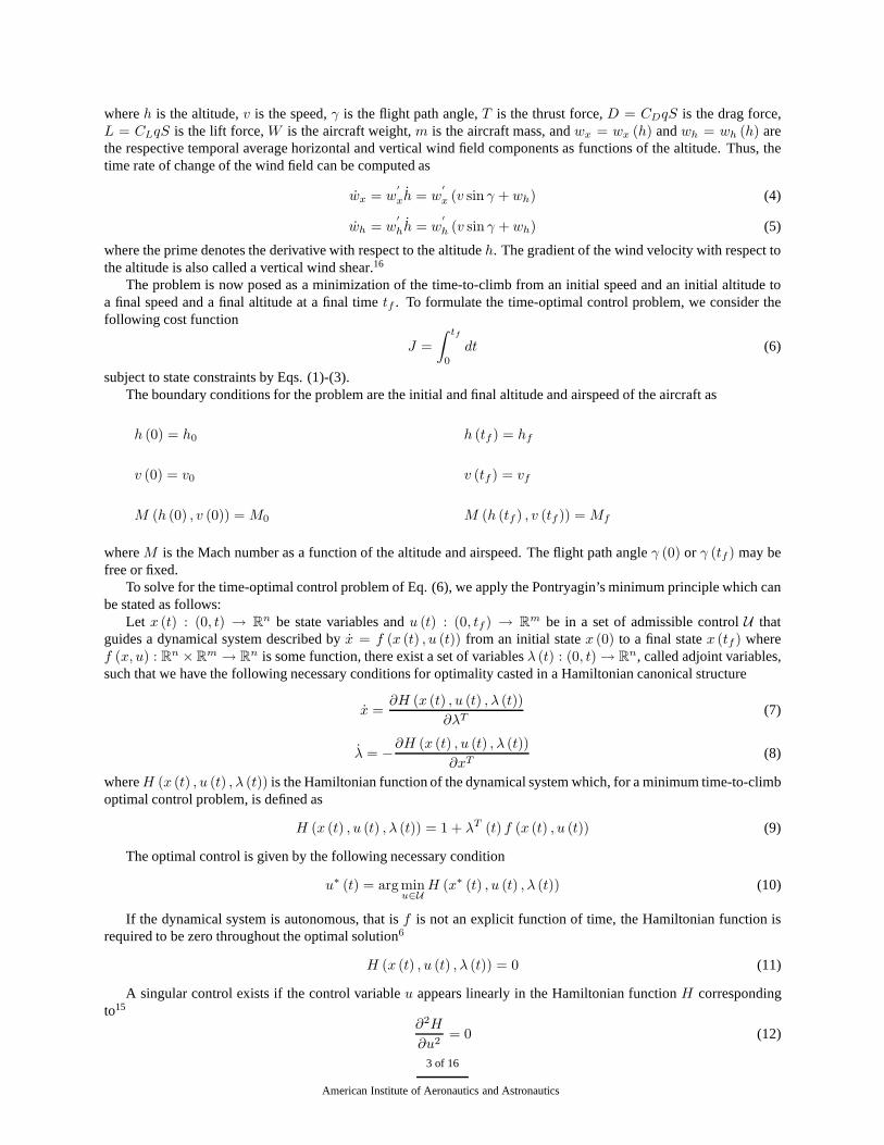
whereh is the altitude,v is the speed,γ is the flight path angle,T is the thrust force,D = CDqS is the drag force,L = CLqS is the lift force,W is the aircraft weight,m is the aircraft mass, andwx = wx (h) andwh = wh (h) arethe respective temporal average horizontal and vertical wind field components as functions of the altitude. Thus, thetime rate of change of the wind field can be computed as

wx = w′

xh = w′

x (v sin γ + wh) (4)

wh = w′

hh = w′

h (v sin γ + wh) (5)

where the prime denotes the derivative with respect to the altitudeh. The gradient of the wind velocity with respect tothe altitude is also called a vertical wind shear.16

The problem is now posed as a minimization of the time-to-climb from an initial speed and an initial altitude toa final speed and a final altitude at a final timetf . To formulate the time-optimal control problem, we consider thefollowing cost function

J =

∫ tf

0

dt (6)

subject to state constraints by Eqs. (1)-(3).The boundary conditions for the problem are the initial and final altitude and airspeed of the aircraft as

h (0) = h0 h (tf ) = hf

v (0) = v0 v (tf ) = vf

M (h (0) , v (0)) = M0 M (h (tf ) , v (tf )) = Mf

whereM is the Mach number as a function of the altitude and airspeed.The flight path angleγ (0) or γ (tf ) may befree or fixed.

To solve for the time-optimal control problem of Eq. (6), we apply the Pontryagin’s minimum principle which canbe stated as follows:

Let x (t) : (0, t) → Rn be state variables andu (t) : (0, tf) → R

m be in a set of admissible controlU thatguides a dynamical system described byx = f (x (t) , u (t)) from an initial statex (0) to a final statex (tf ) wheref (x, u) : R

n ×Rm → R

n is some function, there exist a set of variablesλ (t) : (0, t) → Rn, called adjoint variables,

such that we have the following necessary conditions for optimality casted in a Hamiltonian canonical structure

x =∂H (x (t) , u (t) , λ (t))

∂λT(7)

λ = −∂H (x (t) , u (t) , λ (t))

∂xT(8)

whereH (x (t) , u (t) , λ (t)) is the Hamiltonian function of the dynamical system which, for a minimum time-to-climboptimal control problem, is defined as

H (x (t) , u (t) , λ (t)) = 1 + λT (t) f (x (t) , u (t)) (9)

The optimal control is given by the following necessary condition

u∗ (t) = argminu∈U

H (x∗ (t) , u (t) , λ (t)) (10)

If the dynamical system is autonomous, that isf is not an explicit function of time, the Hamiltonian function isrequired to be zero throughout the optimal solution6

H (x (t) , u (t) , λ (t)) = 0 (11)

A singular control exists if the control variableu appears linearly in the Hamiltonian functionH correspondingto15

∂2H

∂u2= 0 (12)

3 of 16


Let S (x, λ) : Rn × R

n → Rm be a switching function defined by

S =∂H

∂u(13)

Since the controlu does not appear explicitly inS, it cannot be determined explicitly. However, by differentiatingS repeatedly until the controlu appears explicitly, then the controlu is so determined. For the controlu to be optimal,the Kelley’s condition must be satisfied

(−1)k ∂

∂u

(

d2kS

dt2k

)

≥ 0 (14)

For this problem, the Hamiltonian function is defined as

H (h, v, γ, λh, λv, λγT, CL, CD) = 1 + λh (v sin γ + wh) + λv

(

T − D − W sin γ

m− wx cos γ − wh sinγ

)

+ λγ

(

L − W cos γ

mv+

wx sin γ − wh cos γ

v

)

(15)

whereλh, λv, andλγ are the adjoint variables.We define the specific excess thrustF and the wing loading factorn as functions of the altitude, Mach numberM ,

and Reynolds numberRe as

F (h, v, CL) =T [h, M (h, v)] −

{

CD,0 [Re (h, v)] + KC2L

}

q [ρ (h) , M (h, v)] S

W(16)

n (h, v, CL) =CLq [ρ (h) , M (h, v)] S

W(17)

whereCD,0 is the profile drag coefficient andK is the induced drag parameter.Then, the necessary conditions for optimality result in thefollowing adjoint differential equations

λh = −∂H

∂h= −λhw

′

h − λv

[

g∂F

∂h−

(

w′′

x cos γ + w′′

h sin γ)

(v sin γ + wh) −(

w′

x cos γ + w′

h sinγ)

w′

h

]

− λγ

g

v

∂n

∂h+(

w′′

x sin γ − w′′

h cos γ)(

sin γ +wh

v

)

+w

′

h

(

w′

x sin γ − w′

h cos γ)

v

(18)

λv = −∂H

∂v= −λh sin γ − λv

[

g∂F

∂v−

(

w′

x cos γ + w′

h sin γ)

sin γ

]

− λγ

g

v

∂n

∂v−

gn

v2+

g cos γ

v2−

wh

(

w′

x sin γ + w′

h cos γ)

v2

(19)

λγ = −∂H

∂γ= −λhv cos γ − λv

[

−g cos γ − v(

w′

x cos 2γ + w′

h sin 2γ)

+(

w′

x sinγ − w′

h cos γ)

wh

]

− λγ

g sin γ

v+ w

′

x sin 2γ − w′

h cos 2γ +wh

(

w′

x cos γ + w′

h sin γ)

v

(20)

In order to determine the extremal control to achieve a fastest climb path, we take the lift coefficientCL as a controlvariable. Then the optimal control is one that renders the Hamiltonian stationary

∂H

∂CL

= −λv

2KC∗LqS

m+ λγ

qS

mv= 0 ⇒ C∗

L =λγ

2Kvλv

(21)

4 of 16


subject to the inequality constraintCL,min ≤ C∗L ≤ CL,max.

The optimal lift coefficient in Eq. (21) may be solved by a two-point boundary value problem using a numericalmethod such as a shooting method or a gradient descent method. Such a numerical solution often does not reveal astructure of the optimal control analytically. In most cases, it is found that this problem can be approximated as asingular optimal control problem by making an assumption that the induced drag parameterK is usually small andtherefore can be neglected. In fact, the ideal induced drag parameter for an elliptical wing loading is given by

K =1

πAR(22)

whereAR is the aspect ratio. For a typical transport aircraft, the wing aspect ratio is about 7 so that the idealKparameter is about 0.045. Thus, this assumption is reasonable.

Under this assumption, we see that∂2H/∂C2L = 0 and so there exists a singular control with a switching function

S = λγ

qS

mv(23)

SinceqS/mv > 0, we then obtain a bang-bang extremal control as

C∗L =

CL,max λγ < 0

CL,sing λγ = 0

CL,min λγ > 0

(24)

The bang-bang control law is thus viewed as a sub-optimal solution to the minimum time optimal control problem.Equation (24) states that the minimum-time-to-climb trajectory is approximated by three sub-optimal arcs. The firstarc is a trajectory on which the aircraft flies at some initialaltitude and airspeed at a maximum lift coefficient untilit intercepts with a singular arc trajectory defined by the second switching condition. The singular arc is an optimalflight trajectory for the fastest climb8 and is also called an energy climb path (ECP) since it is a paththat crosses a setof level curves of constant energy heightsE = h + v2/2g as illustrated in Fig. 1. At some point on this trajectory, theaircraft climbs out of the singular arc and flies along a final arc with a minimum lift coefficient to arrive at the finalaltitude and airspeed.

To find a singular control, we use the fact thatS = 0 andS = 0 on the singular arc to establish thatλγ = 0 andλγ = 0. Hence, this allows us to eliminateλγ in Eq. (20) by solving forλh

λh = λv

g

v+

w′

x cos 2γ + w′

h sin 2γ

cos γ−

wh

(

w′

x tan γ − w′

h

)

v

(25)

The remaining adjoint equations (18) and (19) now become

λh = λv

{

−g

(

∂F

∂h+

w′

h

v

)

+

[

w′

xw′

h tan γ + w′′

xv cos γ + w′′

hv sin γ −

(

w′

h

)2]

(

sin γ +wh

v

)

}

(26)

λv = λv

[

−g

(

∂F

∂v+

sin γ

v

)

+ sin γ(

w′

x tan γ − w′

h

)(

sin γ +wh

v

)

]

(27)

Differentiating Eq. (25), which is equivalent to computingS = λγ , and then substituting Eq. (27) into the resulting

5 of 16


expression yield

λh = λv

gF

v2

[

−g +(

w′

x tan γ − w′

h

)

wh

]

− g∂F

∂v

g

v+

w′

x cos 2γ + w′

h sin 2γ

cos γ−

wh

(

w′

x tan γ − w′

h

)

v

+gn

v

[

−w′

x sin γ(

3 + tan2 γ)

+ 2w′

h cos γ −w

′

xwh

v cos2 γ

]

+g

v

(

3w′

x tan γ − 2w′

h +2w

′

xwh

v cos γ

)

+

−

2(

w′

x

)2

tan γ

cos γ

(

sin γ +wh

v

)

+w

′

xw′

h

cos γ

(

3 sinγ + 2wh

v

)

−

(

w′

h

)2

(

sin γ +wh

v

)

+

w′′

x cos 2γ + w′′

h sin 2γ

cos γ−

wh

(

w′′

x tan γ − w′′

h

)

v

(

sin γ +wh

v

)

(28)

By equating Eq. (28) to Eq. (26), the singular arc for a minimum time-to-climb is now obtained as

f (h, v, γ, n) = (1 − a1)F + (1 + a2) v∂F

∂v−

v2

g

∂F

∂h+ a3n + a4 = 0 (29)

with the coefficientsa1, a2, a3, anda4 described by the following functions of the wind field parameters

a1 =wh

(

w′

x tan γ − w′

h

)

g(30)

a2 =v(

w′

x cos 2γ + w′

h sin 2γ)

g cos γ−

wh

(

w′

x tanγ − w′

h

)

g(31)

a3 =v

g

[

w′

x sin γ(

3 + tan2 γ)

− 2w′

h cos γ +w

′

xwh

v cos2 γ

]

(32)

a4 =

(

v sin γ + wh

g

)2

2w′

x

(

w′

x tan γ − w′

h

)

cos γ+ v

(

w′′


h

)

−v

g

(

3w′

x tanγ − w′

h +2w

′

xwh

v cos γ

)

(33)

Equation (29) is a partial differential equation in terms ofthe specific excess thrustF that describes an optimalclimb path for a minimum time-to-climb solution for an aircraft flying in the presence of an altitude dependent at-mospheric wind field. Examining Eq. (29) reveals that there is a high degree of cross coupling between the horizontalwind field and the vertical wind field up to the second derivatives of the wind fields. Thus, not only the wind fieldgradients affect the optimal climb path, but the wind field curvatures also play a role as well. Equation (29) resultsin a parabolic equation in terms ofCL, which can be solved to give a feedback control for the lift coefficient on thesingular arc as a function of the three state variablesh, v, andγ.

A certain simplification of Eq. (29) can be made by considering the concept of fast and slow states in flightdynamics. Ardema had shown that in optimal trajectory analysis, the three-state model of a point mass aircraft exhibitsa time-scale separation behavior whereby the state variablesh andv possess slower dynamics than the state variableγ.3 This time scale separation is normally treated by a singularperturbation analysis by replacing the fast state equationwith the following equation

εγ =L − W cos γ

mv+

wx sinγ − wh cos γ

v(34)

whereε is a small parameter.Equation (34) has an inner solution and an outer solution, which is the steady state solution obtained by setting

ε = 0. The inner solution can usually be solved by the method of matched asymptotic expansion. The inner solutionis also called a boundary-layer solution in reference to thehistorical origin of the singular perturbation method inthe fluid boundary layer theory. The overall solution is dominated by the outer solution with the inner solution only

6 of 16


affecting a small initial time period. As a first order approximation, the inner solution can sometimes be ignored. Inthis case, Eq. (34) results in the following load factor

n = cos γ −

(v sin γ + wh)(

w′

x sin γ − w′

h cos γ)

g(35)

Equation (35) thus dethrones the number of state equations from three to two by converting the state variableγinto a control variable in place of the lift coefficientCL. Substituting Eq. (35) into Eq. (29) now yields the optimalclimb path function

f (h, v, γ) = F

1 −

wh

(

w′

x tan γ − w′

h

)

g

+ v∂F

∂v

1 +v(

w′

x cos 2γ + w′

h sin 2γ)

g cos γ−

wh

(

w′

x tan γ − w′

h

)

g

−v2

g

∂F

∂h−

v

g

(

2w′

x sin2 γ tan γ + w′

h cos 2γ +w

′

xwh

v cos γ

)

+ v

(

v sin γ + wh

g

)2(

w′′


h

)

+v

g

(

v sin γ + wh

g

)

(

w′

x tan γ − w′

h

)

(

−w′

x tan γ cos 2γ + 2w′

h cos2 γ +w

′

xwh

v cos γ

)

= 0 (36)

We have thus reduced the optimal climb path by removing the dependency on the lift coefficient. We now examinesome special cases of the general optimal climb path function f (h, v, γ):

1. Steady Wind Field:For a steady wind field, the gradients and curvatures vanish,thereby reducing the optimal climb path functionto the following

f (h, v) = F + v∂F

∂v−

v2

g

∂F

∂h= 0 (37)

Equation (37) is the well-known result for the ECP without anatmospheric wind field. Thus, the optimal climbpath in the presence of a steady wind field is effectively the same as that without the wind field effect. This resultis not surprising and can be explained by the fact that since the inertial reference frame is attached to the airmass, whether the air mass is moving at a constant speed or remains stationary, the speed of the aircraft relativeto the air mass is the same, thus resulting in the same optimalclimb path.

2. Horizontal Wind Field:In the presence of a horizontal wind field only, the optimal climb path function becomes

f (h, v, γ) = F + v∂F

∂v

(

1 +vw

′

x cos 2γ

g cos γ

)

−v2

g

∂F

∂h−

2vw′

x sin2 γ tanγ

g+

v3w′′

x sin2 γ tanγ

g2

−

v2

(

w′

x

)2

g2sinγ tan2 γ cos 2γ = 0 (38)

Specializing Eq. (38) for small flight path angles by invoking sin γ ≈ γ andcos γ ≈ 1 yields

f (h, v) = F + v∂F

∂v

(

1 +vw

′

x

g

)

−v2

g

∂F

∂h−

2vw′

x

g−

v3w′′

x

g2+

v2

(

w′

x

)2

g2

γ3 = 0 (39)

3. Vertical Wind Field:

7 of 16


In the presence of a vertical wind field only, Eq. (36) becomes

f (h, v, γ) = F

(

1 +whw

′

h

g

)

+ v∂F

∂v

(

1 +vw

′

h sin 2γ

g cos γ+

whw′

h

g

)

−v2

g

∂F

∂h−

vw′

h cos 2γ

g

− vw′′

h

(

v sin γ + wh

g

)2

−

2v(

w′

h

)2

cos2 γ

g

(

v sin γ + wh

g

)

= 0 (40)

For small flight path angles, Eq. (40) reduces to

f (h, v, γ) = F

(

1 +whw

′

h

g

)

+ v∂F

∂v

(

1 +2vw

′

hγ + whw′

h

g

)

−v2

g

∂F

∂h−

vw′

h

g− vw

′′

h

(

vγ + wh

g2

)2

−

2v(

w′

h

)2

g

(

vγ + wh

g

)

= 0 (41)

Vertical wind field is especially important for microburst problems. A microburst is a wind shear disturbancecharacterized by an unusually strong downdraft near the ground surface that presents an extreme hazard toaircraft during take-off or landing.

III. Optimal Solution

During a climb, the aircraft flies under a maximum continuousthrust from take-off to a point in the flight trajectoryenvelope where it intersects with the optimal climb path. The aircraft then maintains its course along the optimal climbpath until it reaches some point on the optimal climb path where it climbs out to the final altitude and airspeed. Thus,there exist three climb segments during a climb as illustrated in Fig. 1 labeled as A, B, and C where B is the singulararc optimal climb path. The suboptimal solutions for the climb segments A and C may be defined by lines of constantenergy heightsE = h + v2/2g.11

From the optimal control perspective, the initial and final climb segments are to be determined by requiring theHamiltonian function as defined in Eq. (15) to be zero. In addition, the adjoint variableλγ is no longer restrictedto zero according to the first and last switching conditions in Eq. (24). Thus, in general, the optimal solutions forthe initial and final flight segments are considerably more complex than the optimal climb path solution and usuallyinvolve solving a two-point boundary value problem.

First, we shall consider the singular arc optimal solution.Along this singular arc, all the state and adjoint variablesare functions of the altitudeh, airspeedv, and flight path angleγ. However, it can easily be shown that the flight pathangleγ on the singular arc optimal energy climb path is in turn a function of the altitudeh and airspeedv. Therefore,the two variablesh andv uniquely determine the optimal climb path. In particular, for the case of small flight pathangles for which Eqs. (39) and (41) apply. The optimal climb functionf (h, v, γ) can be written as

f (h, v, γ) =

3∑

n=0

fi (h, v) γi = 0 (42)

wherefi are explicit functions ofv andh.The time derivative off (h, v, γ) is evaluated as

f =

3∑

i=0

(

∂fi

∂hh +

∂fi

∂vv

)

γi (43)

taking into account that the assumptionγ = 0 is built into the climb path function.Substituting Eqs. (1)-(3) into Eq. (43) then yields the following polynomial equation that can be solved for the

flight path angleγ

c5γ5 + c4γ

4 +

3∑

i=0

ci (h, v) γi = 0 (44)

8 of 16


where the coefficientsci are

c5 (h, v) = −∂f3

∂vvw

′

h (45)

c4 (h, v) =∂f3

∂hv −

∂f3

∂v

(

vw′

x + whw′

h + g)

−∂f2

∂vvw

′

h (46)

ci (h, v) =∂fi

∂hwh +

∂fi

∂v

(

Fg − whw′

x

)

+∂fi−1

∂hv −

∂fi−1

∂v

(

vw′

x + whw′

h + g)

−∂fi−2

∂vvw

′

h (47)

Equation (44) gives the flight path angle as a function of the altitude and speed. Thus the optimal climb surfacefunction f (h, v, γ) can be replaced by a climb path functionf (h, v, γ (h, v)) upon embedding the solution of theflight path angle from Eq. (44).

The adjoint variables along the optimal climb path are now determined from enforcing the conditionsH = 0 andλγ = 0 on the singular arc as

λh = −g + vw

′

x + 2vw′

hγ − whw′

xγ + whw′

h

gv (F − γ) + (vγ + wh)(

g + vw′

hγ − whw′

xγ + whw′

h

) (48)

λv = −v

gv (F − γ) + (vγ + wh)(

g + vw′

hγ − whw′

xγ + whw′

h

) (49)

The foregoing analysis has shown that the along the singulararc, the time optimal trajectory is known in thev − hplane as well as the flight path angle and the adjoint variables. This information greatly facilitates the optimal solutionsfor the climb segments on the initial and final arcs. Since theinitial conditions on the initial climb segment are knownaccording to the problem statement and the fact that its solution must terminate on the optimal climb path functionfor which all the state and adjoint variables are known, thenthe optimal solution for the initial arc can be computedusing a shooting technique to integrate backward from some point B on the optimal climb path to the initial pointA as shown in Fig. 1. Likewise, to compute the optimal solution for the final arc, a shooting method may be usedto integrate forward from some point C on the optimal climb path to the final point D that terminates at the desiredaltitude and airspeed. A shooting method may be establishedas follows:

The flight path angleγ not on the optimal climb path function can be solved by setting the Hamiltonian in Eq. (15)to zero with the usual small angle assumption, thus resulting in the following quadratic equation

λvvw′

hγ2 +[

λhv − λv

(

g + vw′

x − whw′

h

)]

γ + 1 + λhwh + λv

(

Fg − whw′

x

)

= 0 (50)

Equation (50) is then used to eliminate the flight path angle expression in the adjoint equation in the adjointdifferential equations (18) and (19), which can then be parameterized in terms of the altitude as the independentvariable instead of time using the following transformation with the small angle assumption

dλh

dh=

λh

h=

−λhw′

h − λv

[

g ∂F∂h

−

(

w′′

x + w′′

hγ)

(vγ + wh) −(

w′

x + w′

hγ)

w′

h

]

vγ + wh

(51)

dλv

dv=

λv

h=

−λhγ − λv

[

g ∂F∂v

−

(

w′

x + w′

hγ)

γ]

vγ + wh

(52)

In addition, the airspeed can also be parameterized as a function the altitude as

dv

dh=

v

h=

(F − γ) g

vγ + wh

− w′

x + w′

hγ (53)

Equations (50)-(53) are then integrated either forward or backward using the known state and adjoint variables onthe optimal climb path as the starting values at points B and C. The shooting method then iterates on these knownvalues on the optimal climb path until the conditions at points A and D are met.

9 of 16


IV. Numerical Example

We compute the time optimal climb trajectory of a transport aircraft in a horizontal wind field. The aircraft has amaximum thrustTmax which varies as a function of the altitude as

T = Tmax

(

ρ

ρ0

)a

(54)

whereρ is the density,ρ0 is the density at the sea level, anda is a constant.Using Eq. (35) with the small flight path angle approximation, the specific excess thrust is computed as

F =Tmax

W

(

ρ

ρ0

)a

−CD

1

2ρv2S

W(55)

The optimal climb path function, Eq. (39), is equal to

f (v, h) =Tmax

W

(

ρ

ρ0

)a(

1 −av2

ρg

dρ

dh

)

−CD

1

2ρv2S

W

(

2 −v2

ρg

dρ

dh+

2vw′

x

g

)

−

2vw′

x

g−

v3w′′

x

g2+

v2

(

w′

x

)2

g2

γ3 = 0 (56)

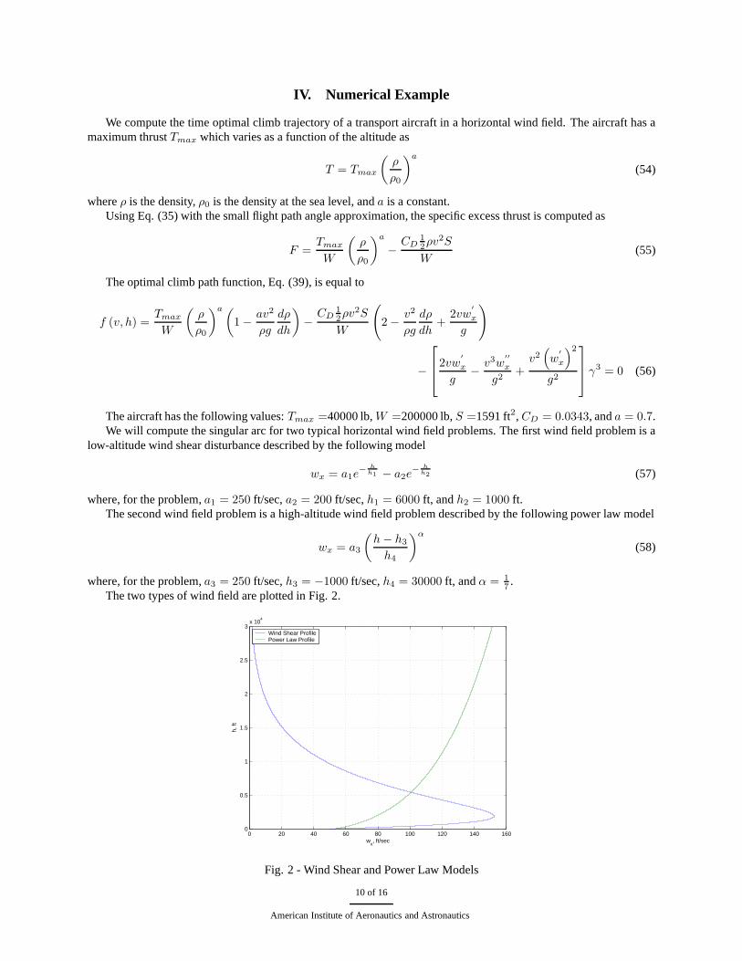
The aircraft has the following values:Tmax =40000 lb,W =200000 lb,S =1591 ft2, CD = 0.0343, anda = 0.7.We will compute the singular arc for two typical horizontal wind field problems. The first wind field problem is a

low-altitude wind shear disturbance described by the following model

wx = a1e− h

h1 − a2e− h

h2 (57)

where, for the problem,a1 = 250 ft/sec,a2 = 200 ft/sec,h1 = 6000 ft, andh2 = 1000 ft.The second wind field problem is a high-altitude wind field problem described by the following power law model

wx = a3

(

h − h3

h4

)α

(58)

where, for the problem,a3 = 250 ft/sec,h3 = −1000 ft/sec,h4 = 30000 ft, andα = 1

7.

The two types of wind field are plotted in Fig. 2.

0 20 40 60 80 100 120 140 1600

0.5

1

1.5

2

2.5

3x 10

4

wx, ft/sec

h, ft

Wind Shear ProfilePower Law Profile

Fig. 2 - Wind Shear and Power Law Models

10 of 16


As can seen, the wind shear profile is characterized by a strong wind field gradient near the ground which can behazardous to aircraft during take-off and landing.

To find the singular arc, we decompose the optimal climb path function, Eq. (56), in the individual functionsfi (h, v) according to Eq. (42). For a horizontal wind field problem, Eq. (44) is then formulated as a4th degreepolynomial function in terms of the flight path angleγ. A physically correct root is obtained that yields the flightpath angle on the singular arc. The singular arc functionf (h, v) then becomes a nonlinear function in terms ofhandv. To compute the singular arc trajectory in thev − h plane, we find the zero solution of this function using aNewton-Raphson method as follows:

vi+1 = vi −

[

df (hi, vi)

dv

]−1

f (hi, vi) (59)

The computed singular arc time-optimal climb paths for bothwind field profiles are plotted in Fig. 3. For reference,we also compute the singular arc for zero wind disturbance. As can be seen, the singular arc climb paths are steeppaths that rapidly increase the altitude with a relatively smaller change in the air speed for the case of no wind. Thepower law profile follows a similar pattern as the no-wind case, although the ground speed intercept is less. Thiswould mean that with the power law profile, the aircraft has toenter the singular arc climb path at lower speed thanif there were no wind. The singular arc for the wind shear profile is the most interesting in that the speed variation issignificant over a wide range at a very low altitude. This is due to the strong wind field gradient over a short altitude.At high altitude, the three singular arcs are converging, sothe effect of wind field is less pronounced at high altitude.

300 350 400 450 500 550 600 6500

0.5

1

1.5

2

2.5

3x 10

4

v, ft/sec

h, ft

No WindWind Shear ProfilePower Law Profile

Fig. 3 - Singular Arc Time-Optimal Climb Paths

Once the singular arc has been determined, the values ofh andv along the singular arc are plugged into the4th

degree polynomial to solve for the flight path angle along thesingular arc. The lift coefficients are also computed.Figs. 4 and 5 are the plots of the flight path angle and lift coefficient on the singular arc climb paths. The flight pathangle for the no-wind case generally decreases with altitude. At high altitude, the flight path angle for the two windprofiles converge to that of the no-wind case. The wind shear case as usual shows a drastic change in the flight pathangle along the singular arc at low altitude. The lift coefficient generally increases with altitude for the no-wind case.The lift coefficient for the wind shear case varies greatly atvery low altitude and is quite large at ground level due tothe low ground speed intercept required to enter the climb path.

We next compute a complete trajectory from take-off to some final altitude and air speed. We only consider thewind shear case. The initial ground speed at take-off is about Mach 0.2 or 224 ft/sec and the desired air speed at15000 ft is Mach 0.5 and 0.6. The solutions not on singular arcrequire solving a two-point boundary value problem.However, since the adjoint variables are completely determined on the singular arc, we can solve the trajectory off thesingular arc quite easily using a shooting method by integrating Eqs. (51) to (53) either forward or backward startingfrom the singular arc. The adjoint solution on the singular arc is plotted in Fig. 6.

11 of 16


1.5 2 2.5 3 3.5 4 4.5 5 5.5 6 6.50

0.5

1

1.5

2

2.5

3x 10

4

γ, deg

h, ft


Fig. 4 - Flight Path Angle on Singular Arc

0.2 0.3 0.4 0.5 0.6 0.7 0.8 0.9 10

0.5

1

1.5

2

2.5

3x 10

4

CL

h, ft


Fig. 5 - Lift Coefficient on Singular Arc

0 0.5 1 1.5 2 2.5 3

x 104

−0.7

−0.6

−0.5

−0.4

−0.3

−0.2

−0.1

0

h, ft

λ v, sec

2 /ft

0 0.5 1 1.5 2 2.5 3

x 104

−0.055

−0.05

−0.045

−0.04

−0.035

−0.03

−0.025

−0.02

λ h, sec

/ft

h, ft

Fig. 6 - Adjoint Solution on Singular Arc

12 of 16


The complete trajectory is plotted in Fig. 7. To climb to 15000 ft and Mach 0.5, the climb trajectory is comprisedof three segments. The first segment, segment AB, is the take-off segment on which the aircraft flies from take-offground speed to intercept the singular arc at point B. This occurs at a very low altitude. The second segment, orsingular arc segment BC, is the minimum-time to climb path that takes the aircraft to a higher altitude in a fastest time.At some point on this singular arc, the aircraft begins to depart at point C and flies on the final segment, segment CD,to the final altitude and airspeed. We note that the three segments join together and are tangent at points B and C. Onthis path, the departure slope is to the left of the singular arc. In the region to the left of the singular arc, because thealtitude is continuously increasing, the thrust is maintained at the maximum value.

The situation for Mach 0.6 corresponding to the final segmentEF is different. Since the aircraft must arrive atMach 0.6 which is to the right of the singular arc. Because thedeparture slope must be tangent to the singular arc andcurve to the left, there is no point below the final altitude where this tangency exists. As a result, the aircraft must flypast the final altitude and then reduce the engine thrust to let the potential energy be convert to kinetic energy once theaircraft begins to slow down. For the problem, we use a first-order model to describe the engine thrust reduction fromthe maximum value to an idle value at roughly 20% of the maximum thrust. The segment EF is sub-optimal in that theengine thrust varies so that it becomes a control variable inaddition to the flight path angle. Nonetheless, it is a verygood approximation since the segment EF approximately follows a total energy curve.

200 250 300 350 400 450 500 550 600 6500

0.5

1

1.5

2

2.5

3x 10

4

v, ft/sec

h, ft

Singular ArcTake−Off SegmentFinal Segment to Mach 0.5Final Segment to Mach 0.6

A

B

C

D E

F

Fig. 7 - Climb Trajectory

0.2 0.4 0.6 0.8 1 1.2 1.4 1.6 1.80

0.5

1

1.5

2

2.5

3x 10

4

CL

h, ft

Singular ArcTake−Off SegmentFinal Segment to Mach 0.5Final Segment to Mach 0.6

A

B

C

D E

F

Fig. 8 - Lift Coefficient on Climb Trajectory

13 of 16


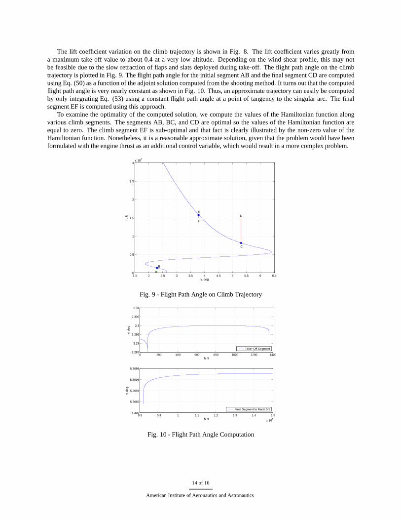
The lift coefficient variation on the climb trajectory is shown in Fig. 8. The lift coefficient varies greatly froma maximum take-off value to about 0.4 at a very low altitude. Depending on the wind shear profile, this may notbe feasible due to the slow retraction of flaps and slats deployed during take-off. The flight path angle on the climbtrajectory is plotted in Fig. 9. The flight path angle for the initial segment AB and the final segment CD are computedusing Eq. (50) as a function of the adjoint solution computedfrom the shooting method. It turns out that the computedflight path angle is very nearly constant as shown in Fig. 10. Thus, an approximate trajectory can easily be computedby only integrating Eq. (53) using a constant flight path angle at a point of tangency to the singular arc. The finalsegment EF is computed using this approach.

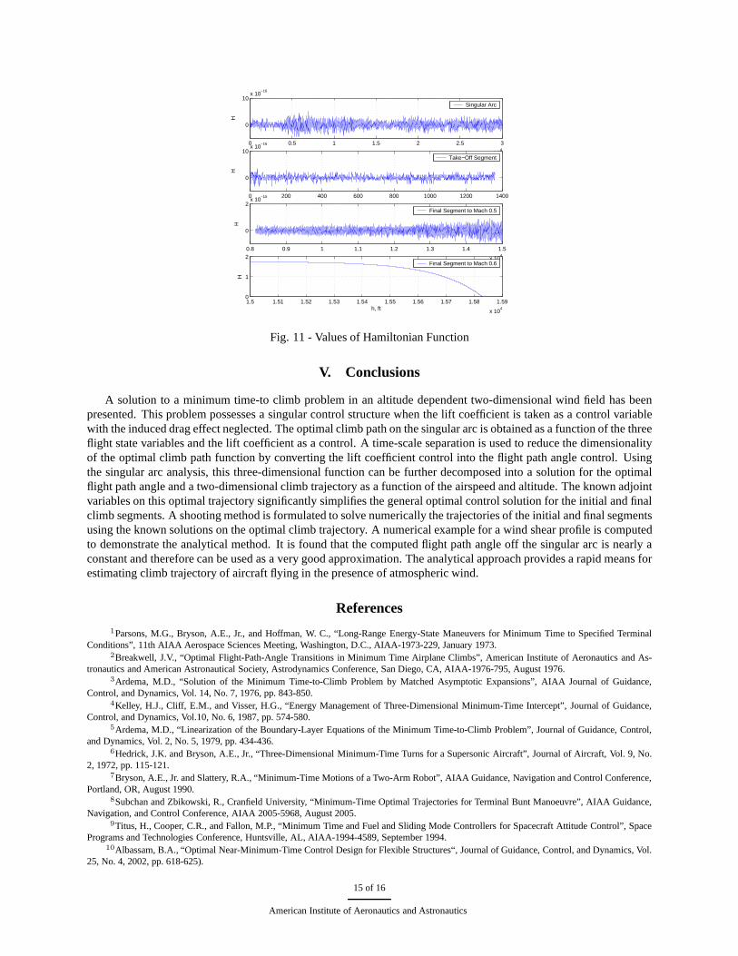
To examine the optimality of the computed solution, we compute the values of the Hamiltonian function alongvarious climb segments. The segments AB, BC, and CD are optimal so the values of the Hamiltonian function areequal to zero. The climb segment EF is sub-optimal and that fact is clearly illustrated by the non-zero value of theHamiltonian function. Nonetheless, it is a reasonable approximate solution, given that the problem would have beenformulated with the engine thrust as an additional control variable, which would result in a more complex problem.

1.5 2 2.5 3 3.5 4 4.5 5 5.5 6 6.50

0.5

1

1.5

2

2.5

3x 10

4

γ, deg

h, ft

A

B

C

D E

F

Fig. 9 - Flight Path Angle on Climb Trajectory

0 200 400 600 800 1000 1200 14002.285

2.29

2.295

2.3

2.305

2.31

h, ft

γ, d

eg

0.8 0.9 1 1.1 1.2 1.3 1.4 1.5

x 104

5.309

5.3092

5.3094

5.3096

5.3098

h, ft

γ, d

eg

Take−Off Segment

Final Segment to Mach 0.5

Fig. 10 - Flight Path Angle Computation

14 of 16


1.5 1.51 1.52 1.53 1.54 1.55 1.56 1.57 1.58 1.59

x 104

0

1

2

h, ft

H

0 0.5 1 1.5 2 2.5 3

x 104

0

10x 10

−16

H

0 200 400 600 800 1000 1200 1400

0

10x 10

−16

H

0.8 0.9 1 1.1 1.2 1.3 1.4 1.5

x 104

0

2x 10

−15

H

Singular Arc

Take−Off Segment



Fig. 11 - Values of Hamiltonian Function

V. Conclusions

A solution to a minimum time-to climb problem in an altitude dependent two-dimensional wind field has beenpresented. This problem possesses a singular control structure when the lift coefficient is taken as a control variablewith the induced drag effect neglected. The optimal climb path on the singular arc is obtained as a function of the threeflight state variables and the lift coefficient as a control. Atime-scale separation is used to reduce the dimensionalityof the optimal climb path function by converting the lift coefficient control into the flight path angle control. Usingthe singular arc analysis, this three-dimensional function can be further decomposed into a solution for the optimalflight path angle and a two-dimensional climb trajectory as afunction of the airspeed and altitude. The known adjointvariables on this optimal trajectory significantly simplifies the general optimal control solution for the initial and finalclimb segments. A shooting method is formulated to solve numerically the trajectories of the initial and final segmentsusing the known solutions on the optimal climb trajectory. Anumerical example for a wind shear profile is computedto demonstrate the analytical method. It is found that the computed flight path angle off the singular arc is nearly aconstant and therefore can be used as a very good approximation. The analytical approach provides a rapid means forestimating climb trajectory of aircraft flying in the presence of atmospheric wind.

References1Parsons, M.G., Bryson, A.E., Jr., and Hoffman, W. C., “Long-Range Energy-State Maneuvers for Minimum Time to Specified Terminal

Conditions”, 11th AIAA Aerospace Sciences Meeting, Washington, D.C., AIAA-1973-229, January 1973.2Breakwell, J.V., “Optimal Flight-Path-Angle Transitionsin Minimum Time Airplane Climbs”, American Institute of Aeronautics and As-

tronautics and American Astronautical Society, Astrodynamics Conference, San Diego, CA, AIAA-1976-795, August 1976.3Ardema, M.D., “Solution of the Minimum Time-to-Climb Problem by Matched Asymptotic Expansions”, AIAA Journal of Guidance,

Control, and Dynamics, Vol. 14, No. 7, 1976, pp. 843-850.4Kelley, H.J., Cliff, E.M., and Visser, H.G., “Energy Management of Three-Dimensional Minimum-Time Intercept”, Journal of Guidance,

Control, and Dynamics, Vol.10, No. 6, 1987, pp. 574-580.5Ardema, M.D., “Linearization of the Boundary-Layer Equations of the Minimum Time-to-Climb Problem”, Journal of Guidance, Control,

and Dynamics, Vol. 2, No. 5, 1979, pp. 434-436.6Hedrick, J.K. and Bryson, A.E., Jr., “Three-Dimensional Minimum-Time Turns for a Supersonic Aircraft”, Journal of Aircraft, Vol. 9, No.

2, 1972, pp. 115-121.7Bryson, A.E., Jr. and Slattery, R.A., “Minimum-Time Motions of a Two-Arm Robot”, AIAA Guidance, Navigation and ControlConference,

Portland, OR, August 1990.8Subchan and Zbikowski, R., Cranfield University, “Minimum-Time Optimal Trajectories for Terminal Bunt Manoeuvre”, AIAA Guidance,

Navigation, and Control Conference, AIAA 2005-5968, August 2005.9Titus, H., Cooper, C.R., and Fallon, M.P., “Minimum Time andFuel and Sliding Mode Controllers for Spacecraft Attitude Control”, Space

Programs and Technologies Conference, Huntsville, AL, AIAA-1994-4589, September 1994.10Albassam, B.A., “Optimal Near-Minimum-Time Control Design for Flexible Structures“, Journal of Guidance, Control, and Dynamics, Vol.

25, No. 4, 2002, pp. 618-625).

15 of 16


11Vinh, N.X., Flight Mechanics of High-Performance Aircraft, Cambridge University Press, 1993.12Pontryagin, L., Boltyanskii, U., Gamkrelidze, R., and Mishchenko, E.,The Mathematical Theory of Optimal Processes, Interscience, 1962.13Leitmann, G.,The Calculus of Variations and Optimal Control, Springer, 2006.14Naidu, D.S. and Calise, A.J., “Singular Perturbations and Time Scales in Guidance and Control of Aerospace Systems: A Survey”, Journal

of Guidance, Control, and Dynamics, Vol. 24, No. 6, 2001, pp.1057-1078.15Bryson, A., and Ho, Y.,Applied Optimal Control: Optimization, Estimation, and Control, Hemisphere Publishing Co., 1975.16Nelson, R.C.,Flight Stability and Automatic Control, McGraw-Hill, 1997.

16 of 16


singular arc time-optimal climb trajectory of … (nguyen).pdfsingular arc time-optimal climb...

Documents