singular value decomposition on processor arrays with a pipelined bus system

Journal of Network and Computer Applications (1996) 19, 235–248

Singular value decomposition on processor arrayswith a pipelined bus system

Yi Pan∗ and Mounir Hamdi†

∗Computer Science Department, University of Dayton, Dayton, OH 45469-2160, USAand †Computer Science Department, Hong Kong University of Science and Technology,Clear Water Bay, Kowloon, Hong Kong

Singular value decomposition (SVD) is used in many applications such as real-timesignal processing where fast computation of these problems is needed. In this paper,parallel algorithms for solving the singular value decomposition problem are discussed.The algorithms are designed for optically interconnected multiprocessor systems wherepipelined optical buses are used to connect processors. In a pipelined bus system,messages can be transmitted concurrently in a pipelined fashion. However, certainrestrictions may apply in a pipelined bus system. For example, a processor can send atmost one message and receive one message during a bus cycle. Pipelined bus in-terconnection requires us to rethink how we write parallel algorithms. Fully exploringthe properties of concurrent message transmissions requires careful mapping of data,an efficient addressing mechanism, and a set of efficient basic data movement operations.In this paper, these issues are addressed in detail. Analysis of the parallel computationtimes of the SVD algorithms shows that they are asymptotically equivalent to thoseimplemented on the hypercube while using substantially less hardware. The resultsobtained in this paper further demonstrate that optically interconnected multiprocessorsystems are very promising as a new multiprocessor architecture.

1996 Academic Press Limited

1. Introduction

One of the important problems in mathematical science and engineering is singularvalue decomposition (SVD). It is often used in many applications such as real-timesignal processing, where the solution to these problems is needed in the shortest possibletime. SVD is one of the most important factorization of a real m-by-n (m≥n) matrix,and is a very computationally intensive problem. Given the growing availability ofparallel computers and the need for faster solutions to the SVD problem, there hasbeen great interest in the development of parallel implementations of the singular valuedecomposition.

A singular value decomposition of a real m-by-n (m≥n) matrix A is its factorizationof this matrix into the product of three matrices:

A=UDVT

where U is an m-by-n matrix with orthogonal columns, D is an n-by-n non-negativediagonal matrix, and V is an n-by-n orthogonal matrix. For more details, please referto Golub and Reisch [1]. The most common method used for the solution of the SVDproblem is incorporated in the Golub–Kahan SVD algorithm [1,2], which requires

2351084–8045/96/030235+14 $18.00/0 1996 Academic Press Limited

236 Y. Pan and M. Hamdi

O(mn2) time on a single processor computer. In order to reduce the computation timeof this sequential algorithm, there has been much interest recently in developing fasterparallel SVD [2–9]. On a linear processor array, the most efficient SVD algorithm isthe Jacobi-like algorithm given by Brent and Luk [3]. The algorithm, which is basedon a one-sided orthogonalization method due to Hestenes [10], takes O(mnS) time onO(n) processors where S is the number of sweeps. However, Brent and Luk’s algorithmis not optimal in terms of communication overhead. Unnecessary costs are incurredby mapping the systolic array architecture onto a ring connected linear array due tothe double sends and receives required between pairs of neighboring processors.Eberlein [11], Bischof [12] and others have proposed various modifications of thisalgorithm for hypercube implementations, which require the embedding of rings viabinary reflected Gray Codes. Gao and Thomas [13] have investigated this problem usinga recursive divide-exchange communication pattern. These algorithms have the sameorder of magnitude of time complexity as the one described by Brent and Luk,but reduce the constant factor. SVD algorithms on hypercube and shuffle-exchangecomputers have also been designed by Pan and Chuang [14]. Instead of mapping acolumn of data onto a processor in a hypercube, as is done in Chuang and Chen [5]and Gao and Thomas [13], they map a column pair of data onto a column of processorsin a hypercube or a shuffle-exchange computer. Using this method, the total time isreduced to O(n log m) per sweep using (mn)/(2 log m) processors.

Most of the parallel algorithm of the SVD problem has been targeted to be executedon point-to-point parallel architectures. The data transmission in these architectures isquite different from that on arrays of processors with pipelined optical buses. One ofthe unique features of a pipelined optical bus is its ability to allow the currenttransmission of messages in a pipelined fashion while having a very short end-to-endmessage delay. This makes it very efficient in the connection of parallel computers. Forthis reason, arrays of processors with pipelined optical buses have attracted a lot ofattention from researchers recently. We will briefly introduce this novel architecture inSection 3. Many important parallel algorithms have been implemented on such anarchitecture, such as broadcasting [15], sorting [16], selection [17], numericalproblems [18], and Hough transform [19]. In this paper, we use this novel architecturefor the implementation of efficient parallel algorithms for the SVD problem.

This paper is organized as follows. Hestenes’ method for solving the SVD problemis reviewed in the next section. In Section 3, a parallel SVD algorithm, which is basedon the Hestenes method, is implemented on a 1-D array of processors with a pipelinedoptical bus. In Section 4, a variation of this parallel algorithm is implemented on a 2-D array of processors with pipelined optical buses. In Section 5, oversized SVD problemsare discussed. Section 6 gives a summary and assessment of our results.

2. Singular value decomposition

There is a wealth of serial SVD algorithms available in the literature. Most of thesealgorithms can be transformed into parallel algorithms to be run on parallel computers.Each of these serial algorithms exhibits a certain degree of parallelism. Thus, in choosingthe serial algorithm to be transformed into a parallel algorithm, we have to take thepotential of inherent parallelism within the algorithm into account. For this reason,we choose the Hestenes method of solving the SVD problem [10] to implement it on

SVD on arrays with a pipelined bus system 237

the array of processors with optical pipelined buses because of its high potential ofparallelism and its flexibility in being transformed efficiently into a parallel algorithmsuited for our architecture, even though its sequential version is less efficient than thatof the Golub–Kahan–Reinsch SVD method [1,2].

The basic idea of the decomposition is to generate an orthogonal matrix V such thatthe transformed matrix AV=W has orthogonal columns. Normalizing the Euclideanlength of each non-null column to unity, we get the relation

W=U′D (1)

where U′ is a matrix whose non-null columns form an orthonormal set of vectors, andD is a non-negative diagonal matrix. An SVD of A is then given using the followingrelation:

A=WVT=U′DVT (2)

As a null column of U′ is always associated with a zero diagonal element of D, (1) and(2) are essentially identical.

Hestenes [10] uses plane rotations to construct V. A sequence of matrices {Ak} isgenerated by

Ak+1=AkRk (k=1, 2, 3, . . .)

where A1=A, and each Rk is a plane rotation. Let Ak=(ak1, ak

2, . . . , akn), where ak

i is theith column of Ak. Suppose Rk=(rk

ij) is a rotation on the (p, q) plane which orthogonalizescolumns ak

p and akq of Ak with p<q. Rk is an orthogonal matrix with all of its elements

identical to those of the unit matrix except that

rkpp=cos h rk

pq=sin h(3)

rkqp=−sin h rk

qq=cos h

We note that post-multiplication of Ak by Rk affects only columns akp and ak

q, and that

(ak+1p , ak+1

q )=(akp, ak

q)C cos h−sin h

sin hcos hD (4)

The rotation angle h should be chosen so that the two new columns are orthogonal.For this we can use the formulas given by Rutishauser [20]. Defining:

c=(akp)Tak

q, a=(akp)Tak

p, b=(akq)Tak

q (5)

We set h=0, if c=0. Otherwise, we compute

L=b−a

2c,t=

sign(L)|L |+J1+L2

(6a)


0 1 N–1

Directional CouplerProcessor

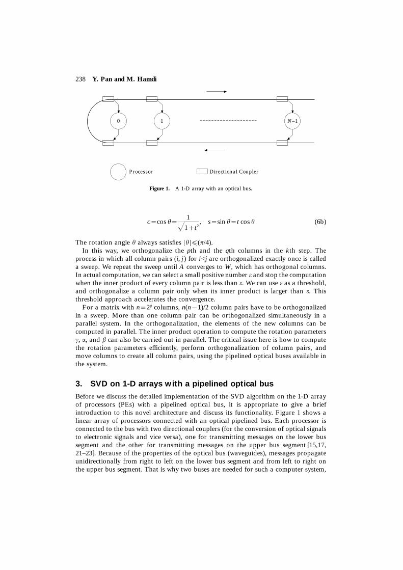
Figure 1. A 1-D array with an optical bus.

c=cos h=1

J1+t2, s=sin h=t cos h (6b)

The rotation angle h always satisfies |h |≤(p/4).In this way, we orthogonalize the pth and the qth columns in the kth step. The

process in which all column pairs (i, j ) for i<j are orthogonalized exactly once is calleda sweep. We repeat the sweep until A converges to W, which has orthogonal columns.In actual computation, we can select a small positive number e and stop the computationwhen the inner product of every column pair is less than e. We can use e as a threshold,and orthogonalize a column pair only when its inner product is larger than e. Thisthreshold approach accelerates the convergence.

For a matrix with n=2g columns, n(n−1)/2 column pairs have to be orthogonalizedin a sweep. More than one column pair can be orthogonalized simultaneously in aparallel system. In the orthogonalization, the elements of the new columns can becomputed in parallel. The inner product operation to compute the rotation parametersc, a, and b can also be carried out in parallel. The critical issue here is how to computethe rotation parameters efficiently, perform orthogonalization of column pairs, andmove columns to create all column pairs, using the pipelined optical buses available inthe system.

3. SVD on 1-D arrays with a pipelined optical bus

Before we discuss the detailed implementation of the SVD algorithm on the 1-D arrayof processors (PEs) with a pipelined optical bus, it is appropriate to give a briefintroduction to this novel architecture and discuss its functionality. Figure 1 shows alinear array of processors connected with an optical pipelined bus. Each processor isconnected to the bus with two directional couplers (for the conversion of optical signalsto electronic signals and vice versa), one for transmitting messages on the lower bussegment and the other for transmitting messages on the upper bus segment [15,17,21–23]. Because of the properties of the optical bus (waveguides), messages propagateunidirectionally from right to left on the lower bus segment and from left to right onthe upper bus segment. That is why two buses are needed for such a computer system,


unlike traditional electronic buses where electronic signals can propagate in eitherdirection on the same bus. Each processor uses a set of control registers to storeinformation needed to control the transmission and reception of messages by thatprocessor which will be explained later. The above computer system can operate inMIMD mode where each processor would have its own controller, or in SIMD modewhere a single controller is used for all the processors. In this paper, this parallelcomputer system is assumed to be operating in SIMD mode, and thus our algorithmsare designed with this mode in mind.

For convenience, we let the optical path length between any two couplers on the busbe d0 units. Denote the propagation time of a light signal between two couplers by tc;that is, tc=d0/cg, where cg is the velocity of light on the bus. Let a bus cycle, Tc, beNtc. With a concurrent bus accessing method, often referred to as bus pipelinings [21,22], processors can transmit their messages simultaneously at the beginning of eachbus cycle. As a result of a simultaneous transmission by all processors, a train of Nmessages is formed on the lower segment of the bus and will propagate from left toright on the upper segment. Processors that wish to receive any message from amongthe train of messages transmitted must wait for the message to arrive at its receiver [23].These properties are a result of the unique characteristics of optical buses (waveguides).For more details, readers are referred to Melhem et al. [22].

Messages transmitted by different processors may overlap with each other even if theypropagate unidirectionally on the bus. We call these message overlappings transmissionconflicts. Assume each message has b binary bits, where each bit is represented by anoptical pulse, with the existence of a pulse for 1 and the absence of a pulse for 0. Letw be the width (or duration) of each pulse in seconds. To ensure free of transmissionconflicts, the following condition has to be satisfied:

tc>bw (7)

We call tc a pipeline cycle; thus, the term pipelined bus is self-explanatory. The abovecondition ensures that each message will be ‘fit’ into a pipeline cycle such that, in abus cycle, up to N messages can be transmitted by processors simultaneously withoutcollisions on the bus. This is the biggest difference between an optical bus and electronicbus, where the former can handle up to N simultaneous messages when connected ton processors while the latter can handle just one message regardless of the number ofprocessors. In a parallel array, messages normally have very short length (b is verysmall). Thus, in the remaining discussions, we assume that the condition given by eqn(7) above is always satisfied and no transmission conflicts are possible as long as allprocessors are synchronized at the beginning of each bus cycle.

In SIMD environments, each processor knows the source (processor id) of themessage it is receiving and when it is sent relative to the beginning of a bus cycle.Therefore, the time (relative to the beginning of a bus cycle) can be easily calculatedby the processor receiving the message. Let the processor that wishes to receive amessage be processor i. Assume that the message is sent by processor j at the beginningof bus cycle C. We use a receiving function, rec(i, j, C), to determine the time thatprocessor i has to wait, relative to the beginning of bus cycle C, before receiving themessage from processor j. The value of the function, in the number of pipeline cycles,is given in the following equation:


rec(i, j, C)=i+j+1 (8)

By calculating the receiving function as given by eqn (8), each processor would beable to selectively receive any message from a train of messages in each bus cycle.These values of receiving functions can be precomputed and stored in a set ofreceiving control registers for fast retrieval during the execution of the algorithm. Theprecomputing of these values is done, obviously, according to the design of the givenalgorithm. Readers may refer to Melhem et al. [22] for details.

Now, it is time to present the SVD algorithm on the 1-D array with an optical busof size n/2, in which every PE has a local memory large enough to store a pair ofcolumns of data elements. Suppose that the two columns are stored in arrays A(i )and B(i ), 0≤i<n/2, respectively. Every PE continuously receives commands from thecontroller to perform the orthogonalization of the column pair concurrently with otherPEs according to eqns (3–6). A procedure called 1-D-ORTH is used to orthogonalizea column pair as follows. 1-D-ORTH consists of the following steps, i.e. to update a,c, and b using (5), to calculate L, t, c, and s using (6), and to orthogonalize the columnpair based on (4). Since the length of a column is m, it takes O(m) to update (5). Allother steps in 1-D-ORTH can be done in constant time. Hence, the time to perform1-D-ORTH is O(m).

After performing the orthogonalization of the column pair, each PE exchanges acolumn of data with another PE. Clearly, any exchange of column data between twoPEs can be done in m bus cycles since each PE can put one message onto the bus andreceive one message from the bus in one bus cycle and a column contains m dataelements. Here, the exchange sequence described in Dekel et al. [24] is used to movedata column A(i ) in PE[i ], for all i, to all other PEs sequentially to produce all (A, B)column pairs, i.e. the set {(Ap, Bq) |p=0, 1, 2, . . . , n/2−1, q=0, 1, 2, . . . , n/2−1}. Inorder to obtain all possible column pairs, one still has to consider the pairing amongthe A columns and among the B columns. This can be achieved by iteratively applyingthe process of exchanging the A and the B columns between neighboring nodes tocreate subarrays and then moving the A columns within the subarrays. The entirealgorithm is given in procedure 1-D-SVD.

procedure 1-D-SVD1 While not (all |c |<e) do2 1-D-ORTH;3 for k :=0 step 1 until g−1 do4 for p :=1 step 1 until 2g−k−1 do5 h :=f (g−k, p);6 Rrc(i )←1+i+i (h);7 for j :=1 step 1 until m do8 Bus←A[ j ](i );9 A[ j ](i )←Bus;10 end for j ;11 1-D-ORTH;12 end for p;13 if rk=0 then14 Rrc(i )←1+i+i (h);


15 for j :=1 step 1 until m do16 Bus←B[ j ](i );17 A[ j ](i )←Bus;18 end for j ;19 else20 Rrc(i )←1+i+i(h);21 for j :=step 1 until m do22 Bus←A[ j ](i );23 B[ j ](i )←Bus;24 end for j ;25 1-D-ORTH;26 end for k;27 end while;

In the above algorithm, f (g−k, p) is the pth number in the exchange sequence [24]of length 2g−k−1. i (h) is the number whose binary representation is iq, . . . , ih, . . . , i0.Rrc(i ) is the receiving control register used to store the receiving function value inprocessor i. Thus, when Rrc(i ) is assigned the value of 1+i+i (h), processor i receives amessage automatically from processor i (h). A[ j ](i ) is the j th element of the data columnstored in processor i. Column pairs are generated within a subarray by loop p usingthe exchange sequence [25]. Lines 13 to 24 iteratively exchange the A and B columnsbetween neighboring nodes. Obviously, lines 8, 9, and 11 dominate the time complexityof the algorithm since they are statements within the double loop. The time spent inprocedure 1-D-ORTH on line 11 is O(m) since each PE needs to process a column pairwhose length is m. The number of times line 11 is executed is given by:

]g−1

k=0A ]

2g−k−1

p=1

1B=An2−1B+An4−1B+An8−1B · · ·+1≤n.

(9)

Hence, the time spent in line 11 is O(mn). Similarly, it can be shown that the numberof times lines 8 and 9 are executed is

]g−1

k=0

m(2g−k−1)

=mGAn2−1B+An4−1B+An8−1B · · ·+1H (10)

≤mn

Thus, the time spent in lines 8 and 9 is O(mn). Therefore, the total time of algorithm1-D-SVD is O(mn), which is on the same order of magnitude as that on a hypercubeof the same size [5]. While a PE in a linear array of size n with a pipelined optical bushas only two communication ports, a PE in a hypercube of size n has log n ports.


Figure 2. A 2-D array with row and column optical buses.

4. SVD on 2-D arrays with pipelined optical buses

The 1-D array with a single pipelined optical bus has certain limitations [23]. First, thesystem size cannot be very large since it is limited by the minimum power that can bedetected by the PE at the very end of the bus (similar to electronic buses). Second,when the number of PEs, N, is very large, the end-to-end transmission delay increasessince the condition given by eqn (3) has to be held and the number of pipeline cyclesis proportional to N. Moreover, many problems, such as SVD, are 2-D in nature andare more efficient when implemented on a 2-D array of processors. To overcome theshortcomings of the linear array of processors, we consider a 2-D array of processorswhere each row of processors and each column of processors are connected by apipelined optical bus. Thus, a PE in a 2-D array is coupled to four waveguides: twofor transmitting messages and two for receiving messages (see Fig. 2). Communicationbetween PEs in the same row or in the same column in a 2-D array can be carried thesame way as in the linear case. If two PEs in different rows or different columns needto communicate, then two bus cycles are needed. That is, at the end of the first buscycle a message has to be buffered at a node which is in the same row (or column) asthe destination [15,21–23]. It is expected that parallel algorithms can be run moreefficiently on a 2-D array than on a 1-D array as can be deduced from our SVDalgorithms implemented on a 1-D array and a 2-D array. Nevertheless, a 1-D arraywith a pipelined optical bus is a legitimate architecture with its own merits [22].

Now we consider the implementation of the SVD problem on the 2-D array ofprocessors with pipelined optical buses of size m×(n/2), where n=2g+1. Each PE in arow has an index which is between [0, m−1] and each PE in a column has an indexwhich is between [0, n/2−1]. Hence, each PE can be uniquely identified by its row indexand column index. Each PE(i, j ) has several registers; registers A(i, j ) and B(i, j ) areused to store matrix elements. The given matrix A is initially stored as follows:

A(i, j )=aij, B(i, j )=ai,(n/2)+j , for 0≤i<m, 0≤j<n/2 (11)


where aij is the (i, j ) element of matrix A. Thus, the n columns of the matrix arepartitioned into n/2 pairs and each column pair is stored in a column of m processors.

A column of m processors orthogonalizes the column pair stored in it by using theprocedure 2-D-ORTH explained below. The procedure 2-D-ORTH is similar to 1-D-ORTH except that a column pair of data is stored in a column of processors insteadof one processor. 2-D-ORTH is divided into several distinct phases and each phasecorresponds to its counterpart in 1-D-ORTH. In the first phase, the local products

c(i, j )=A(i, j )∗B(i, j ) 0≤i<m

a(i, j )=A(i, j )∗A(i, j ) 0≤i<m (12)

b(i, j )=B(i, j )∗B(i, j ) 0≤i<m

are calculated in the m processors concurrently. In the second phase, the sums

]m−1

i=0

c(i, j ), ]m−1

i=0

a(i, j ), and ]m−1

i=0

b(i, j ) (13)

are computed by combining the partial sums using the reporting operation describedin Hamdi and Pan [18], and the results are stored in PE(0, j ). In the third phase, thevalues L( j ), t( j ), c( j ), and s( j ) are computed locally in P(0, j ). In the fourth phase,the rotation parameters c(0, j )=c( j ) and s(0, j )=s( j ) are broadcast over the columnbuses to all processors in the same columns. The broadcast operation described inHamdi and Pan [18] can be used here. In the fifth phase, elements of the two newmatrix columns are computed locally using the rotation parameters received. The timecomplexity of the 2-D-ORTH can be derived as follows. The first phase takes a constanttime since all operations are local. The second phase needs O(log m) time since theseare reporting operations over columns of m PEs [18]. The third phase uses a constanttime. In the fourth phase, one bus cycle is needed since it is a broadcasting operationover columns [18]. The fifth phase requires a constant time again. Hence, the time takenin 2-D-ORTH is O(log m).

After the procedure 2-D-ORTH is performed in parallel on all n/2 columns ofprocessors, half of the newly computed matrix columns are exchanged in parallelbetween neighboring columns of processors. The procedure 2-D-ORTH is then carriedout on all columns of processors in parallel again. Clearly, any column exchangebetween two PEs can be done in one bus cycle since this is a one-to-one operation.Here again the exchange sequence described in Dekel et al. [24] is used to move columnA[i, j ] in PE[i, j ], for all i and j, to all other PEs sequentially to produce all (A, B)column pairs in a column of PEs, i.e. the set {(Ap, Bq) |p=0, 1, 2, . . . , n/2−1, q=0, 1,2, . . . , n/2−1}. In order to obtain all possible column pairs, one still has to considerthe pairing among the A columns and among the B columns. This can be achieved byiteratively applying the process of exchanging the A and the B columns betweenneighboring columns of PEs to create subsystems and then moving the A columnswithin the subsystems. The entire algorithm is very similar to its 1-D counterpart andis specified in 2-D-SVD:


procedure 2-D-SVD1 While not (all |c |<e) do2 2-D-ORTH;3 for k :=0 step 1 until g−1 do4 for p :=1 step 1 until 2g−k−1 do5 h :=f (g−k, p);6 Rrc(i, j )←1+i+i(h);7 RowBust(i )←A(i, j );8 A(i, j )←RowBus(i );9 2-D-ORTH;10 end for p;11 if rk=0 then12 Rrc(i,j )<−1+i+i(h);13 RowBus(i )←B(i, j );14 A(i, j )←RowBus(i );15 else16 Rrc(i,j )←1+i+i(h);17 RowBus(i )←A(i, j );18 B(i, j )←RowBus(i );19 2-D-ORTH;20 end for k;21 end while;

In the 2-D-SVD algorithm, A(i, j ) and B(i, j ) denote memory locations withinprocessor (i, j ). RowBus(i ) is the optical bus at row i in the array. All the other symbolshave the same meaning as described in the 1-D-SVD algorithm. The algorithm is similarto the 1-D-SVD except that a column pair is mapped onto a column of processors inthe 2-D-SVD instead of onto a single processor. The time spent in procedure 2-D-ORTH is O(log m) as analysed before. Most time of the algorithm is spent within thedouble loop (lines 5 to 9). Since lines 5 and 6 require a constant time and each datatransfer in lines 7 and 8 takes one bus cycle, the time is dominated by line 9. Similarto the analysis of the 1-D-SVD algorithm, the number of times line 9 is executed is atmost n. Therefore the total time of 2-D-SVD is O(n log m), which is on the same orderof magnitude as that on a hypercube of the same size [14]. While a PE in a 2-D arraywith a pipelined optical bus has only four communication ports, a PE in a hypercubeof size mn/2 has log(mn/2) ports.

5. Large SVD problems

Finally, let us discuss the time complexity of the parallel SVD algorithm on an arraywhere the number of processors is much smaller than the size of the problem. Supposewe have a 2-D v×w array with optical pipelined buses. Without loss of generality,suppose v≤m and w≤n. Also assume that m and n are multiples of v and w, respectively.We partition the m-by-n matrix A into h groups of w columns each: C1, C2, . . . , Ch, asshown in Fig. 3 for h=3. In this example, all column pairs which are orthogonalizedin a sweep can be obtained by pairing the columns in the following way: (C1, C1), (C1,C2), (C1, C3), (C2, C2), (C2, C3). Therefore, the whole computation consists of processing


m C1 C2 C3

w w ww

n

Figure 3. Column groups in a large matrix.

all pairs of column groups by algorithm 2-D-SVD. To process a pair of column groups,m/v matrix columns are stored in each column of processors with m/v pairs of matrixelements stored in the local memory of each processor. O(w(log v+m/v) ) time is requiredto process a pair of column groups because each processor has to perform m/vmultiplications and additions locally, and the summation of partial sums and thebroadcast of parameters within a column of processors each requires O(log v) time.The number of pairs of column groups is

h+(h−1)+(h−2)+· · ·+2+1=h(h+1)/2 (14)

where h=n/w. Thus, the total time required to compute a sweep of SVD for an m×nmatrix is O( (h(h+1)/2)w(log v+m/v) )=O(nh(log v+m/v) ) on a 2-D v×w array withoptical pipelined buses. For large SVD problems on a 1-D array with optical pipelinedbuses, similar analysis can be applied. Assume that a 1-D array with optical pipelinedbuses has w processors, h(h+1)/2 pairs of column groups need to be processed, whereh=n/w. To process a pair of column groups, each processor has to process w columnpairs. The time to process each column pair is O(m). Hence, the time required toprocess a sweep of SVD for an m×n matrix is O( (h(h+1)/2)mw) which is (hmn).


6. Conclusions

Parallel computers using static networks such as the mesh and hypercube have theproblem of large diameters due to their limited connectivities. The time complexitiesof parallel algorithms on these networks are lower bounded by their diameters. Addingbuses to these networks is one way to solve the problem. However, messages cannotbe transmitted concurrently on an electronic bus. A pipelined optical bus, on the otherhand, not only has a shorter end-to-end propagation delay, but also can be accessedconcurrently by messages. It has been established that much higher bandwidth can beachieved with pipelined optical bus communication than with exclusive electronic busaccess communication [21]. Thus, many parallel algorithms can be implemented on anarray with a pipelined optical bus efficiently. In this paper, we have shown that thetime complexities used in the algorithms on arrays with optical interconnects areasymptotically equivalent to those implemented on the hypercube while they usesubstantially less hardware.

In this paper, we have concentrated on algorithm design on the optical bus system.During the description of the singular value decomposition algorithms and the opticalbus system, many assumptions from Qiao and Melhem [23] are used. Many technicaldetails such as clock distribution, frame synchronization, electronically controlledoptical switching, conversion between optical and electronic signals, and packet sizelimitation are either discussed briefly or completely omitted. Interested readers mayrefer to references [15,17,21,23,25] for details.

Recently, the authors have proposed another new computational model calledLinear Array with a Reconfigurable Pipelined Bus System (LARPBS) based on opticalwaveguides [26]. In this model, messages can be transmitted in a pipelined fashion onan optical bus system and the bus can be dynamically reconfigured into independentsegments to satisfy different communication requirements during a computation. Usingconditional optical delays, many basic operations such as binary prefix summation,split, compression, and multiple broadcasting can be done in one bus cycle [26]. It isclear that LARPBS is much more powerful than the model used in this paper althoughonly several switches are added to a pipelined optical bus system. We believe that theSVD problem can be solved more efficiently on the LARPBS and we are doing researchin this direction.

References

1. G. H. Golub and C. Reisch 1971. Singular value decomposition and least squares solutions.In Handbook for Automatic Computation, Vol. 2 (Linear Algebra) (J. H. Wilkinson and C.Reinsch, eds), 134–151. New York: Springer-Verlag.

2. G. H. Golub, W. Kahan and F. T. Luk 1980. Computing the singular-value decompositionon the ILLIAC-IV. ACM Transactions on Mathematical Software, 6, 524–539.

3. R. P. Brent and F. T. Luk 1985. The solution of singular-value and symmetric eigenvalueproblems on multiprocessor arrays. SIAM Journal of Scientific and Statistical Computation,6, 69–84.

4. R. P. Brent, F. T. Luk and C. F. Van Loan 1985. Computation of the singular valuedecomposition using mesh-connected processors. Journal of VLSI Computer Systems, 1,243–270.

5. Henry Y. H. Chuang and L. Chen 1989. Efficient computation of the singular valuedecomposition on cube connected SIMD machine. Supercomputing ’89, 276–282, Reno,November.


6. A. M. Finn, F. T. Luk and C. Pottle 1982. Systolic array computation of the singular valuedecomposition. Proceedings of the SPIE Symposium, 341, Real Time Signal Processing V,35–43.

7. D. E. Heller and I. C. F. Ispen 1982. Systolic networks for orthogonal equivalencetransformations and their applications. Proceedings 1982 Advanced Research in VSLI, MIT,Cambridge, pp. 113–1convolution22.

8. F. T. Luk 1984. A triangular processor array for computing the singular value decomposition.TR84-625, Computer Science Department, Cornell University.

9. R. Schreiber 1983. A systolic architecture for singular value decomposition. Proceedings 1stInternational Colloquium on Vector and Parallel Computing in Scientific Applications, Paris,143–148.

10. M. R. Hestenes 1958. Inversion of matrices by biorthogonalization of related results. Journalof Social and Industrial Applied Mathematics, 6, 51–90.

11. P. J. Eberlein 1987. On using the Jacobi method on the hypercube. SIAM Proceedings of theSecond Conference on Hypercube Multiprocessors, 605–611.

12. C. Bischof 1987. The two-sided Jacobi method on a hypercube. SIAM Proceedings of theSecond Conference on Hypercube Multiprocessors, 612–618.

13. G. R. Gao and S. J. Thomas 1988. An optimal parallel Jacobi-like solution method for thesingular value decomposition. Proceedings of the 1988 International Conference on ParallelProcessing, 47–53, August.

14. Yi Pan and Henry H. Y. Chuang 1992. Highly parallel algorithms for singular valuedecomposition on hypercube SIMD machines. Computers and Mathematics with Applications,24, 23–32.

15. C. Qiao, R. Melhem, D. Chiarulli and S. Levitan 1991. Optical multicasting in linear arrays.International Journal of Optical Computing, 2, 31–48.

16. Z. Guo 1992. Sorting on array processors with pipelined buses. 1992 International Conferenceon Parallel Processing, 289–292, St. Charles, IL, August 17–21.

17. Y. Pan 1994. Order statistics on optically interconnected multiprocessor systems. The FirstInternational Workshop on Massively Parallel Processing Using Optical Interconnections,162–169, Cancun, Mexico, April 26–27. (Also in the Special Issue on Optical Computing,Optics and Laser Technology, 26, 281–287, 1994.)

18. M. Hamdi and Y. Pan 1995. Efficient parallel algorithms for some numerical problems onarrays with pipelined optical buses. IEE Proceedings – Computers and Digital Techniques,142, 87–92, March.

19. Y. Pan 1992. Hough transform on arrays with an optical bus. Fifth International Conferenceon Parallel and Distributed Computing and Systems, 161–166, Pittsburgh, PA, October 1–3.

20. H. Rutishauser 1971. The Jacobi method for real symmetric matrices. In Handbook forAutomatic Computation, Vol. 2 (C. Reinsch, ed.), 202–211. Berlin: Springer-Verlag.

21. Z. Guo, R. Melhem, R. Hall, D. Chiarulli and S. Levitan 1991. Array processors withpipelined optical buses. Journal of Parallel and Distributed Computing, 12, 269–282.

22. R. Melhem, D. Chiarulli and S. Levitan 1989. Space multiplexing of waveguides in opticallyinterconnected multiprocessor systems. Computer Journal, 32, 362–369.

23. C. Qiao and R. Melhem 1993. Time-division optical communications in multiprocessorarrays. IEEE Transactions on Computers, 42, 577–590, May.

24. E. Dekel, D. Nassimi and S. Sahni 1981. Parallel matrix and graph algorithms. SIAM Journalof Computing, 10, 657–675.

25. D. Chiarulli, R. Melhem and S. Levitan 1987. Using coincident optical pulses for parallelmemory addressing. IEEE Computer, 20, 48–58.

26. Yi Pan and Mounir Hamdi 1994. Quicksort on a linear array with a reconfigurable pipelinedbus system. Working Paper 94-03, Center for Business and Economics Research, Universityof Dayton.


Yi Pan was born in Jiangsu, China, on May 12, 1960. He enteredTsinghua University in March 1978 with the highest college entranceexamination score of all 1977 high school graduates in Jiangsu Province.He received his BEng degree in computer engineering from TsinghuaUniversity, China, in 1982, and his PhD degree in computer sciencefrom the University of Pittsburgh, USA, in 1991.

Since 1991, he has been an assistant professor in the Department ofComputer Science at the University of Dayton, Ohio, USA. His researchinterests include parallel algorithms and architectures, distributed com-puting, task scheduling, and networking. He has published 12 papers inrefereed international journals and many papers in various internationalconferences. He has received several awards including Research Op-portunity Award from the US National Science Foundation, AndrewMellon Fellowship from the Mellon Foundation, and Summer ResearchFellowship from the Research Council of the University of Dayton. Hisresearch has been supported by the US National Science Foundationand US Air Force.

Dr Pan is a member of the IEEE Computer Society and the Associationfor Computing Machinery.

Dr Hamdi received the BSc degree with distinction in Electrical En-gineering from the University of Southwestern Louisiana in 1985, andMSc and PhD degrees in Electrical Engineering from the University ofPittsburgh in 1987 and 1991, respectively. While at the University ofPittsburgh, he was a Research Fellow in various research projects oninterconnection networks, high-speed communication, parallel al-gorithms, and computer vision. In 1991 he joined the Computer ScienceDepartment at the Hong Kong University of Science and Technologyas an Assistant Professor. His main areas of research are parallelcomputing, high-speed networks, and ATM packet switching ar-chitectures. Dr Hamdi has published over 40 papers on these areas invarious journals and international conferences.

singular value decomposition on processor arrays with a pipelined bus system

Documents