singularity analysis on a planar system with multiple delays

DOI: 10.1007/s10884-006-9063-9Journal of Dynamics and Differential Equations, Vol. 19, No. 2, June 2007 (© 2006)

Singularity Analysis on a Planar Systemwith Multiple Delays

Yuan Yuan1,3 and Junjie Wei2

Received December 13, 2005; revised August 4, 2006

A planar model with multiple delays is studied. The singularities of themodel and the corresponding bifurcations are investigated by using the stan-dard dynamical results, center manifold theory and normal form method ofretarded functional differential equations. It is shown that Bogdanov–Takens(BT) singularity for any time delays, and a serious of pitchfork and Hopfbifurcation can co-existent. The versal unfoldings of the normal forms at theBT singularity and the singularity of a pure imaginary and a zero eigenvalueare given, respectively. Numerical simulations have been provided to illustratethe theoretical predictions.

KEY WORDS: Delay differential equations; singularity; bifurcation; centermanifold; normal form.

1. INTRODUCTION

Recently, the interest in study of the dynamical properties occurringin the neural networks with delay has been growing rapidly (see1,5,9,10,11,13 and the references therein).

Among the numerous research outcome in studying the planar sys-tems representing a network of two neurons, Faria discussed a slightlygeneral delayed system with or without self-connections, and analyzedHopf bifurcation in [3], Bogdanov–Takens (BT) singularity in [4]; Wei and

1 Department of Mathematics and Statistics, Memorial University of Newfoundland,St. John’s, NL, A1C 5S7, Canada. E-mail: [email protected]

2 Department of Mathematics, Harbin Institute of Technology, Harbin, 150001, People’sRepublic of China.

3 To whom correspondence should be addressed.

437

1040-7294/07/0600-0437/0 © 2006 Springer Science+Business Media, Inc.

438 Yuan and Wei

Velarde [11] investigated the following model

u1(t)=−ku1(t)+af (u1(t))+b1g1(u2(t− τ2)),

u2(t)=−ku2(t)+af (u2(t))+b2g2(u1(t− τ1)).

For this system, under the assumption f ′(0)= g′i (0), i = 1,2, they gave a

bifurcation set in an appropriate parameter (b1b2, a)-plane, and pointedout that a Hopf and a BT bifurcations co-occur at the point (b1b2, a)=(0, k) . They did not study the dynamical behavior near the singularityfurther.

The purpose of this paper is to investigate the possible singularitiesand the associated bifurcations for a more general planar system. Realisti-cally, the time delay may exist among any connections due to the informa-tion transmission. By introducing the time delay r in the self-connection,and the delays τi, (i= 1,2) in the connections between different element,we consider the following model

u1(t)=−ku1(t)+af (u1(t− r))+b1g1(u2(t− τ2)),

u2(t)=−ku2(t)+af (u2(t− r))+b2g2(u1(t− τ1)),(1)

where k>0, r�0 and τi �0 (i=1,2), f, g1, g2 ∈C3(R).To simplify the analysis, we assume

(H1) f (0)=g1(0)=g2(0)=0 , f ′(0)=g′1(0)=g′

2(0)=1.

It is obvious that the system (1) has a trivial equilibrium point under thehypothesis (H1). However, if the system has the nontrivial equilibrium, theprocess is similar after a simple transformation.

This paper is organized as follows. We first discuss the multiple stabil-ity and singularity in Section 2, then give the bifurcation analysis in Sec-tion 3. Section 4 presents the numerical simulations. Finally, we draw theconclusions in Section 5.

2. MULTIPLE STABILITIES

The linearized equation of the system (1) is

x1(t)=−k x1(t)+ax1(t− r)+b1x2(t− τ2),

x2(t)=−k x2(t)+ax2(t− r)+b2x1(t− τ1).(2)

The characteristic equation associated with (2) at the equilibrium ori-gin is

�(λ)= (λ+k−ae−λr )2 −b1b2e−2λτ =0, (3)

where τ = τ1+τ22 .

Singularity Analysis on a Planar System 439

Denote � = {(b1b2, a) : a= k− √b1b2, b1b2 � 0}. In �, if b1b2 = 0,

then a=k, Eq. (3) becomes

�1(λ)= (λ+k−ke−rλ)2 =0. (4)

Clearly, all the roots in Eq. (4) are the eigenvalues of the system (1) withthe multiplicity two. If b1b2> 0, then a= k−√

b1b2<k, Eq. (3) can beenrewritten as

λ+k−ae−rλ=±√b1b2e

−λτ . (5)

Obviously, λ= 0 is always a root of Eqs. (3) and (5) if the parameters aand b1, b2 are constrained in �.

In fact, we have the following results when a, b1, b2 lay in theregion �.

Lemma 2.1.

(i) if b1b2 =0, then λ=0 is a double zero root of Eq. (3);(ii) if b1b2> 0 and τ �= τ0 =− 1+ar

k−a � 0, then λ= 0 is a single root ofEq. (3);

(iii) if b1b2>0 and τ =τ0, then λ=0 is a double zero root of Eq. (3).

Proof. In the region �, if b1b2 =0, from a=k, it is obvious that λ=0 is a double zero root by Eq. (4) and

d�1

dλ|λ=0 =0 ,

d2�1

d2λ|λ=0 =2(1+kr)2>0.

If b1b2>0 , a=k−√b1b2<k, then �(0)=0,

d�

dλ|λ=0 =2(k−a)[1+ar+ τ(k−a)].

The fact k > a implies that d�dλ

|λ=0 = 0 if and only if τ = τ0 = − 1+ark−a � 0

since τ �0.By computation directly we have

d2�

dλ2|λ=0, τ=τ0 =2[(1+ar)2 −ar2(k−a)−2b1b2τ

20 ].

Recalling

b1b2τ0 =−(k−a)(1+ar),it follows that

d2�

dλ2|λ=0, τ=τ0 =−2(1+2ar+ar2k)=−2[1+ar+ar(1+ rk)]>0,

since τ0 �0 implies 1+ar <0 and a<0. This completes the proof.

440 Yuan and Wei

Lemma 2.2. All the roots, except λ= 0, in Eq. (3) have negative realparts if either of the following condition is satisfied:

(i) b1b2 =0,(ii) b1b2>0, a�0,

(iii) b1b2>0, a <0, r=0,(iv) b1b2>0, a <0, τ = r.Proof. If the condition (i) is hold, let λ=v+ iω be a root in Eq. (4),

i.e.,

v+ iω+k=ke−rv(cosωr− i sinωr),

then

v+k=ke−rv cosωr , ω=−ke−vr sinωr. (6)

The first equation in (6) implies

(v+k)ervk

= cosωr. (7)

Since k>0 , r�0, then v�0. Thus Eq. (3) has no root with positive realpart. If v=0, from Eq. (6), we have ω2 + k2 = k2, i.e., ω=0. So Eq. (3)has no purely imaginary root. Therefore, all the roots in Eq. (3), exceptλ=0, have negative real part.

(ii) If b1b2>0, a�0, substituting λ=v+ iω into Eq. (5) yields

v+ iω+k−ae−rv(cosωr− i sinωr)=±√b1b2e

−τv(cosωτ − i sinωτ). (8)

Then, v+k=ae−rv cosωr±√b1b2e

−τv cosωτ .From k=a+√

b1b2 , a�0, if v>0,

v+a+√b1b2 =ae−rv cosωr±

√b1b2e

−τv cosωτ �a+√b1b2,

which is meaningless. If v=0, it is derived from Eq. (8) that

k=a cosωr±√b1b2 cosωτ, ω=−a sinωr∓

√b1b2 sinωτ,

then

w2 +k2 = a2 +√b1b2

2 ±2a√b1b2(cosωr cosωτ + sinωr sinωτ)

= a2 +b1b2 ±2a√b1b2 cos(τ − r)ω

� a2 +b1b2 +2a√b1b2 = (a+√

b1b2)2 = k2,

so ω=0. The above process shows that when b1b2>0 , a�0, the conclu-sion is correct.

The proof for (iii) and (iv) is parallel to (i) and (ii), we omit here.


Lemma 2.3. Assume b1b2 > 0, a = k − √b1b2 < 0 and r > r0 = − 1

k+√

1k2 − 1

ak. Then there exist

τ0<τ1< · · ·<τj < · · ·such that Eq. (3) has purely imaginary roots when τ = τj , j =0,1, . . .

Proof. Let λ= iω be a root in Eq. (3) (or Eq. (5)), then from (5)we have

k−a cosωr=±√b1b2 cosωτ

ω+a sinωr=∓√b1b2 sinωτ .

Hence ω solves

ω2 +a2 +k2 +2aω sinωr−2ak cosωr−b1b2 =0. (9)

Denote the left side in Eq. (9) as h(ω), then

h(0)=a2 +k2 −2ak−b1b2 = (k−a)2 −b1b2 =0

from a=k−√b1b2.

Since

h′(ω) = 2[ω+a(1+kr) sinωr+arω cosωr] ,h′′(ω) = 2[1+ar(2+kr) cosωr−ar2ω sinωr],h′(0) = 0 , h′′(0)=2(1+2ar+akr2) .

The assumption r > r0 = − 1k

+√

1k2 − 1

akimplies that h′′(0) < 0 and hence

h′(ω)<0 when ω>0 and ω closes to 0. Therefore h(ω)<0 when ω→0+.On the other hand, limω→+∞ h(ω)=∞. Thus there exists ω0>0 such thath(ω0)=0. We use {ωj } , j =1 , . . . ,m to denote all of the positive root inEq. (9).

Define

τ±lj = 1

ωj

[arccos(±k−a cosωj r√

b1b2)+ lπ

], j =1 , . . . ,m, l=0 ,1 , . . . ,

(10)

then ±iωj is a pair of purely imaginary roots of Eqs. (3) and (5) whenτ = τ±l

j , respectively. Without loss of generality, we can reorder {τ±lj } as

{τj } such that τ0<τ1< · · ·<τj < · · · , the proof is complete.

Lemma 2.4. If b1b2>0, a=k−√b1b2. For fixed r >0 and τ >0, there

exists 0<δ=δ(r, τ )<1 such that all the roots of Eq. (3), except λ=0, havenegative real parts when |a|<δ.

442 Yuan and Wei

Proof. Equation(3) can be rewritten as

λ+k−ae−λr =√b1b2e

−λτ (11)

and

λ+k−ae−λr =−√b1b2e

−λτ . (12)

When a = 0, the assumption implies that k = √b1b2, then Eq. (11)

becomes,

λ+k=ke−λτ .Let λ=α+ iω be its root. Then we have

α+ iω+k=ke−ατ (cosωτ − i sinωτ).

Separating the real and complex parts yields

α+k = ke−ατ cosωτ, (13)

ω = −ke−ατ sinωτ. (14)

From Eq. (13), applying k>0, we have α�0. If α=0, Eq. (13) impliesthat ωτ = 2nπ. Then ω= 0 from Eq. (14). Therefore all the roots of Eq.(11) with a=0, except λ=0, have negative real parts.

By the isolated property of the zeros in an analytic function, there is apositive number γ ∈ (0,1) such that Eq. (11) with a=0 has only one root,λ=0, in the closer of the region B={λ : |λ|<γ }.

Without loss of generality, we consider the case of |a|< 1. Then theroots of Eq. (11) with nonnegative real part satisfy

|λ|<k+1+√b1b2.

Set

={λ :Reλ>0 and |λ|<k+1+√b1b2}∪B.

It follows that Eq. (11) with a= 0 has no root on ∂, the boundaryof , and has only one root, λ = 0, in . By Rouche’s Theorem[2, Theorem 9.17.4], there exists a positive number 0< δ1 < 1 such thatEq. (11) has no root on ∂, and has only one root in when |a|<δ1.This implies that Eq. (11) has only one root with nonnegative real partwhen |a|<δ1. Since λ=0 is always a root to Eq. (11), hence all the rootsof Eq. (11), except λ=0, have negative real parts when |a|<δ1.

Notice that all the roots of the equation λ+k=−ke−λτ have negativereal parts. Similar to the discussion above, we can prove that there exists aconstant δ2>0 such that all the roots of Eq. (12) have negative real partswhen |a|<δ2. Let δ=min{δ1, δ2}. The conclusion follows.


Lemma 2.5.

(i) If b1b2 > 0, k− √b1b2 = a <− 1

r, then Eq. (3) with τ = 0 has a

positive root.(ii) If b1b2>0, k−√

b1b2 =a>− 1r, then all the roots of Eq. (3) with

τ =0, except λ=0, have negative real parts.

Proof. We still rewrite Eq. (3) as Eqs. (11) and (12). Then when τ =0, and k−√

b1b2 =a, Eq. (11) becomes

�0(λ)=λ+a−ae−λr =0,

hence �0(0)= 0, and �′0(λ)

∣∣λ=0 = 1 + ar < 0 if a <− 1

r. From limλ→+∞

�0(λ)=+∞, we know that there exists λ0> 0 such that �0(λ0)= 0. Thisshows that Eq. (11) with τ =0 has at least a positive root, and hence Eq.(3) does.

Similar to the proof of the statement that all the roots of Eq. (11)with |a|<δ1, except λ=0, have negative real parts, in the proof process ofLemma 2.4, we can verify that all the roots of Eq. (11) with τ =0, exceptλ=0, have negative real parts when a>− 1

r.

When τ =0 and√b1b2 =k−a, Eq. (12) becomes

λ+2k−a−aeλr =0. (15)

Let λ=α+ iω be a root, then it follows that

α+2k−a= ae−αr cos(rω),ω= −ae−αr sin(rω).

We can see that the first is meaningless for α� 0 from k >a. This showsthat all the roots of Eq. (14) have negative real parts, and the proof iscomplete.

Summarize the above lemmas, we have the following theorem.

Theorem 2.6. When (b1b2 , a)∈�, in the system (1),

(i) there exists BT bifurcation near the origin if b1b2 =0 , or b1b2>

0, τ = τ0 = − 1+ark−a ; and the dynamical behavior near the origin

is determined by a two-dimensional reduced ordinary differentialequation (ODE);

(ii) when b1b2 > 0, the dynamical behavior near the origin is deter-mined by one or two-dimensional reduced ODE if one of follow-ings is satisfied: (1) a�0; (2) a<0 and r=0; (3) a<0 and τ = r;(4) |a|<δ for fixed r and τ , where δ is given in Lemma 2.4;

444 Yuan and Wei

(iii) there co-exists a zero-purely imaginary singularity at τ =τj (τj isdefined in (10)) if b1b2>0, a<0 and r >r0 (r0 is given in Lemma2.3); Moreover, the dynamical behavior in a neighborhood of theorigin is determined by a three-dimensional reduced ODE whena>− 1

rat τ = τ0;

(iv) the zero solution with τ =0 is unstable when a<− 1r.

If (b1b2, a) is not in �, there is no zero eigenvalues in system (1),and there may have pure imaginary eigenvalues under some restrictions.

Lemma 2.7. If τ = 0, a = k and b1b2 < 0, then Eq. (3) has a pair ofpurely imaginary roots ±iω0 when r= rj , where

ω0 =√

|b1b2|, and rj = 2jπ√|b1b2|, j =0,1, . . .

Proof. Under the given conditions, Eq. (3) becomes

(λ+k−ke−λr )2 =b1b2. (16)

Let iω(ω>0) be a root of Eq. (16), then we have

iω+k−k(cosωr− i sinωr)=±i√

|b1b2|

and hence

k=k cosωr, ω∓√

|b1b2|=−k sinωr .

It follows that

ω=√

|b1b2| def= ω0, rj = 2jπ√|b1b2|, j =0,1, . . .

Let λ(r)=α(r)+ iω(r) be a root of Eq. (16) satisfying

α(rj )=0, ω(rj )=ω0.

Lemma 2.8. If the conditions in Lemma 2.7 are satisfied, then α′(rj )=0,and Eq. (16) has no root with positive real part.

Proof. Substituting λ(r) into Eq. (16) and taking derivative withrespect to r gives

dλ

dr[1+kre−λr ]=−kλe−λr


and

α′(rj )= dλdr

|r=rj =− kλe−λr1+kλe−λr |r=rj

= − ikω0r(cosω0rj−i sinω0rj )

1+krj (cosω0rj−i sinω0rj )

= −i kω01+krj �=0.

The second part of proof is similar to that in Lemma 2.2.Therefore, we have

Theorem 2.9. If τ =0, a=k and b1b2<0, then

(i) all the roots of Eq. (3) have negative real parts when r ∈(rj , rj+1), j =0,1,2, . . . ;

(ii) there exists a pair of purely imaginary roots ±i√|b1b2| at r= rj ,and all the roots of Eq. (3) with r = rj , except ±i√|b1b2|, havenegative real parts.

Remark 2.10. Followed by Lemma 2.8 and Theorem 2.9, we knowthat the degenerate Hopf bifurcation occurs at r= rj , in which the trans-versal condition dλ

dr|r=rj �=0 is invalid. In the study of ordinary differential

equations, the degenerate Hopf bifurcation has been investigated by manyresearchers (see [6,8] and the references therein), but for the delay differ-ential equations, to our best knowledge, there is no any result publishedyet. We leave this study as our future pursuit.

3. BIFURCATION ANALYSIS

To investigate the singularities of the system near the origin, we usethe center manifold theory and the normal form method with unfolding.For an abstract retarded functional differential equation

u=L(μ)ut +F(ut ,μ), (17)

in the phase space C=C([−ν, 0];R2) (ν=max(r, τ1, τ2)), ut (θ)=u(t+θ),−ν�θ�0,μ is the perturbation variable in a neighborhood of zero, L(μ)is a continuous linear map and F is a nonlinear smooth map. To obtainthe center manifold corresponding to the singularity, we use the bilinear form

<ψ,φ>=ψ(0)φ(0)−∫ 0

−ν

∫ θ

0ψ(ξ − θ)dη(θ)φ(ξ)dξ

to decompose C as C = P ⊕Q, where P is an invariant finite dimen-sional subspace and Q is the associated invariant infinite dimensional

446 Yuan and Wei

complementary subspace, and η(θ) is a bounded invariant function.For the system (1),

η(θ)=[−kδ(θ)+aδ(θ − r) b1δ(θ − τ2)

b2δ(θ − τ1) −kδ(θ)+aδ(θ − r)].

By choosing the basis in P , we can obtain the reduced ordinary differen-tial equation in the form x =Bx +�(0)G(�x + y) , here y = y(x(t))∈Q,and MG={ϕ∈C :ϕ=�x(t)+y(x(t))} is the center manifold. Consequently,we can analyze the dynamical behavior of the system based on the reducedODE on the center manifold and further reduction to the normal form, ifnecessary.

3.1. Bogdanov–Takens Bifurcation

From Theorem 2.6, we know that the system (1) undergoes a BTbifurcation in two cases: b1b2 = 0, a = k and b1b2 > 0, τ = τ0 � 0. Wefocus our attention on the bifurcation analysis in detail for the first case.The procedure for the second case is similar, but the computation is muchmore complicated.

Without loss of generality, let b2 = 0 and b1 �= 0. We can choose thebasis for P as

�(θ)= (ϕ1, ϕ2)=[

1 θ

0 cb1

],

where c=1+kr, the basis for the dual space P ∗ in C∗ as

�(s)= col(ψ1, ψ2)=⎡

⎣1c

− b1c3 [c(s+ τ2)−kr2]

0 b1c2

⎤

⎦ .

It is not difficult to verify that �(θ) and �(s) satisfy �(θ)=�(θ)B1 with

B1 =[

0 10 0

],−�(s)=B1�(s) and <�,�>= I . Introducing two parame-

ters μ1 and μ2 and let a = k+μ1 , b2 = 0 +μ2, then system (1) can beexpanded as

u1(t)= −ku1(t)+ (k+μ1)u1(t− r)+b1u2(t− τ2)+F 12 +h.o.t ,

u2(t)= −ku2(t)+ (k+μ1)u2(t− r)+μ2u1(t− τ1)+F 22 +h.o.t , (18)

where F 12 , F

22 are the quadratic terms.

Rewrite (18) as

ut =L(μ)ut +F2(ut , μ)+h.o.t= (L1(μ)+L0)ut +F2(ut , μ)+h.o.t ,(19)


where

L(μ)φ=( −kφ1(0)+ (k+μ1)φ1(−r)+b1φ2(−τ2)

−kφ2(0)+ (k+μ1)φ2(−r)+μ2φ1(−τ1)

)

,

L0φ=(−kφ1(0)+kφ1(−r)+b1φ2(−τ2)

−kφ2(0)+kφ2(−r)

)

,

L1(μ)φ=(

μ1φ1(−r)μ1φ2(−r)+μ2φ1(−τ1)

)

, and

F2(φ)=⎛

⎝af ′′(0)

2 φ21(−r)+b1

g′′1 (0)2 φ2

2(−τ2)

af ′′(0)

2 φ22(−r)

⎞

⎠ .

Then, from φ=�z+y, it follows that

z=B1z+�(0)G1(�z+y, μ), (20)

where y∈Q. To use the lowest order terms in Eq. (20), we can choose y=0,then

G1(�z,μ) = L1(μ)�z+F2(�z, μ)+h.o.t

=(

μ1(�(−r)z)1μ1(�(−r)z)2 +μ2(�(−τ1)z)1

)

+(a2(�(−r)z)21 +b12(�(−τ2)z)

22

a2(�(−r)z)22

)

+h.o.t

with a2 =a f ′′(0)2 , b12 =b1

g′′1 (0)2 , and �(0)=

⎡

⎣1cb1c3 [kr2 − cτ2]

0 b1c2

⎤

⎦ .

Since �z=[

1 θ

0 cb1

]z=

(z1 + θz2cb1z2

), then Eq. (20) becomes

z=B1z+⎛

⎝μ1c(z1 − rz2)+ μ1

c2 (kr2 − cτ2)z2 + b1

c3μ2(kr2 − cτ2)(z1 − τ1z2)

μ1cz2 + b1

c2μ2(z1 − τ1z2)

⎞

⎠

+⎛

⎝a2c(z1 − rz2)

2 + b12b2

1cz2

2 + a2b1 c(kr2 − cτ2)z

22

a2b1z2

2

⎞

⎠+h.o.t . (21)

448 Yuan and Wei

Following the computation of the normal forms for functional differentialequations introduced by Faria and Magalhaes [4], we can get the normalform with versal unfolding on the center manifold

z=B1z+(

0λ1z1 +λ2z2

)+(

0A1z

21 +A2z1z2

)+h.o.t , (22)

where

λ1 = b1

c2μ2, λ2 = (2c−b1τ1)

c2μ1 + b1

c3(kr2 − cτ2)μ2,

A1 =0 , A2 = 2a2

c.

Assembling the information obtained above and applying the centermanifold theorem we have the following result.

Theorem 3.1. If b1b2 = 0, a BT bifurcation occurs in the system (1),and the dynamical behavior of the system (1) near the origin is determinedby (22).

Since A1 =0, we understand that there are no homoclinic curves nearthe origin, while the sink-saddle and source-saddle connections exist.

Remark 3.2. It is well known (see [7,14]) that in BT bifurcation, thesigns of A1, A2 are important in a topological classification, and these twocoefficients must be nonzero for the unfolding to be fully determined. InEq. (22), since A1 = 0, the degenerate BT bifurcation will take place. Aswe know so far, there is no general recipe available for constructing andanalyzing such a family yet.

3.2. Coexistence of Hopf and Transcritical/Pitchfork Bifurcations

When b1b2>0, a=k−√b1b2<0 , r >r0 and τ = τj , from Lemma 2.3,

there exist a single zero and a simple pure imaginary eigenvalues in thesystem (1). If f ′′(0), g′′

1 (0), g′′2 (0) are not zero simultaneously, the trans-

critical and Hopf bifurcations can coexist; otherwise, if f ′′′(0), g′′′1 (0), g

′′′2 (0)

are not zero simultaneously, the pitchfork and Hopf bifurcations can coex-ist. To analyze these bifurcations, we make the following assumption.

(H2) τ1 = τ2def= τ , τ ∗ = r

τis a constant.

By time rescaling, t→ tτ

, the original system (1) becomes

u1(t)= τ [−k u1(t)+a f (u1(t− τ ∗))+b1 g1(u2(t−1))],u2(t)= τ [−k u2(t)+a f (u2(t− τ ∗))+b2 g2(u1(t−1))]. (23)


We can check that, the linearized system

x1(t) = τ [−k x1(t)+ax1(t− τ ∗)+b1x2(t−1)],

x2(t) = τ [−k x2(t)+ax2(t− τ ∗)+b2x1(t−1)]

has a simple zero eigenvalue and a simple pair of pure imaginary eigen-values when τ ∗> r0

τ, a= k−√

b1b2< 0 and τ = τj , where τj = k−a cos ωj τ∗b1b2 cos ωj

,and ωj solves

h(ω)=b1b2ω cosω+ (a sinωτ ∗ −b1b2 sinω)(k−a cosωτ ∗) .

Therefore, the local center manifold near the origin is in a three-dimen-sional subspace.

Fix j , and let τ = τj +μ1 , a=a+μ2, then Eq. (23) can be rewrittenas

u1(t) = (τj +μ1) [−k u1(t)+ (a+μ2) f (u1(t− τ ∗))+b1 g1(u2(t−1))],

u2(t) = (τj +μ1) [−k u2(t)+ (a+μ2) f (u2(t− τ ∗))+b2 g2(u1(t−1))].

(24)

We choose the basis in P as �(θ)= (φ1, φ2, φ3) with φ1 = eiωj θ v, φ2 =φ1, φ3 =v, where

v=(

1γ1

)and γ1 =

√b1b2

b1.

Note: Actually, v can be chosen as(

1±γ1

)depending on λ + τj k −

τj ae−t∗λ=±τj

√b1b2e

−λ. Here, we just consider the case “+”, it is similarfor the case “−”. The basis in Q is given by �(s)= col(ψ1,ψ2,ψ3) withψ1 = e−iωj suT , ψ2 = ψ1, ψ3 = zT , where

u=(d1γ2d1

), z=

(d2γ2d2

), and γ2 =

√b1b2

b2.

Then from <�,�>= I we can determine the values of d1, d2:

d1 = ((1+ 1√b1b2

)(1+aτj τ ∗e−iωj τ∗)+2τj

√b1b2e

−iωj )−1 ,

d2 = ((1+ 1√b1b2

)(1+aτj τ ∗)+2τj√b1b2)

−1 .

Hence the dynamical behavior near the singularity is determined by

u=B2u+�(0)G2(�u,μ) , (25)

450 Yuan and Wei

where

B2 =⎡

⎣i ωj 0 0

0 − i ωj 00 0 0

⎤

⎦ ,

G2(ϕ,μ) = μ1

(−kϕ1(0)+aϕ1(−τ ∗)+b1ϕ2(−1)

−kϕ2(0)+aϕ2(−τ ∗)+b2ϕ1(−1)

)

+μ2

(τj ϕ1(−τ ∗)

τj ϕ2(−τ ∗)

)

+ τj(a2ϕ

21(−τ ∗)+b12ϕ

22(−1)

a2ϕ22(−τ ∗)+b22ϕ

21(−1)

)

+ τj

(a3ϕ

31(−τ ∗)+b13ϕ

32(−1)

a3ϕ32(−τ ∗)+b23ϕ

31(−1)

)

+h.o.t

with a2 = af ′′(0)

2! , b12 = b1g′′

1 (0)2! , b22 = b2

g′′2 (0)2! , a3 = a

f ′′′(0)3! ,

b13 =b1g′′′

1 (0)3! , b23 =b2

g′′′2 (0)3! , and �(0)=

⎡

⎣d1 γ2d1d1 γ2d1d2 γ2d2

⎤

⎦ .

Denote

�u=[eiωj θ e−iωj θ 1eiωj θ γ1 e

−iωj θ γ1 γ1

]⎛

⎝u1u2u3

⎞

⎠=(ξ(θ)

γ1ξ(θ)

),

where ξ(θ)=eiωj θu1 +e−iωj θu2 +u3. We can further reduce Eq. (25) to thenormal form with versal unfolding as

u1 = iωj u1 +m11 u1 +m12 u1u3 +h.o.t ,u2 = − iωj u2 + m11u2 + m12u2u3 +h.o.t ,u3 = m21u3 +m22(u

23 +2u1u2)+h.o.t , (26)

where

m11 = d1(μ1((1+ 1√b1b2

)i ωjτj

+ ( 1√b1b2

−1)e−iωj )+μ2τj (1+ 1√b1b2

)e−iωj τ∗),

m12 = 2d1(a2(1+ 1√b1b2

)e−iωj τ∗ + (γ1b12 +γ2b22)e−iωj ),

m21 = d2(μ1(1√b1b2

−1)+μ2τj (1+ 1√b1b2

)),

m22 = d2(a2(1+ 1√b1b2

)+γ1b12 +γ2b22).

(27)


Using the transformations

⎧⎨

⎩

u1 =w1 + iw2u2 =w1 − iw2u3 =w3

and

⎧⎨

⎩

w1 =ρ cos ζw2 =ρ sin ζw3 = z

subse-

quently, we can change Eq. (26) to real then cylindrical coordinates,

ρ = Re(m11) ρ+Re(m12) z ρ+h.o.t ,ζ = ωj +h.o.t,z = m21 z+m22 (z

2 +2ρ2)+h.o.t . (28)

When Re(m12) ,m22 �=0(note that m22 is real), the higher-order terms haveno qualitative effects. We can check that, if f ′′(0)=g′′

1 (0)=g′′2 (0)=0, then

Re(m12)=m22 = 0, so we need compute the normal form up to the thirdorder, which is,

u1 = iωj u1 +m11 u1 +m13 (u21u2 +u1u

23)+h.o.t ,

u2 = − iωj u2 + m11u2 + m13 (u1u22 +u2u

23)+h.o.t ,

u3 = m21u3 +m23(u33 +6u1u2u3)+h.o.t, (29)

where

m13 = 3d1 (a3(1+ 1√b1b2

)e−iωj τ∗ + (γ1b13 +γ2b23)e

−iωj ) ,

m23 = d2 (a3(1+ 1√b1b2

)+γ1b13 +γ2b23)

and m11 ,m21 are given in (27). In cylindrical coordinates (29) becomes

r= Re(m11) ρ+Re(m13) (ρ3 +ρ z2)+h.o.t,

ζ = ωj +h.o.t,z= m21 z+m23 (z

3 +6 z ρ2)+h.o.t .(30)

Therefore, we have the following conclusion.

Theorem 3.3. If the parameters satisfy the assumption (H2) and a=k − √

b1b2 < 0 , τ ∗ > r0τ

and τ = τj , then the flow of the system (1) onthe local center manifold is given in cylindrical coordinates by (28) whenRe(m12),m22 �= 0; otherwise by (30) when f ′′(0) = g′′

1 (0) = g′′2 (0) = 0 and

Re(m13),m23 �=0.

4. NUMERICAL SIMULATION

To verify our predictions in the previous sections, we choose functionsand parameters satisfying the hypophysis to perform the numerical simu-lations using the dynamical packages XPPAUT and BIFTOOL.

452 Yuan and Wei

-1

-0.8

-0.6

-0.4

-0.2

0

0.2

0.4

0.6

0.8

x2

-1 -0.8 -0.6 -0.4 -0.2 0 0.2 0.4 0.6 0.8x1

-1

-0.8

-0.6

-0.4

-0.2

0

0.2

0.4

0.6

0.8

x1,2

60 80 100 120 140 160 180 200t

(a) (b)

Periodic solutionPhase portrait

Figure 1. Parameters k = 1/3, a = −1, b1 = 1.8, b2 = 1, τ1 = τ2 = 0.5, r = 1.8 with I.C X0 =(0.5, −0.4).

-0.4

-0.2

0

0.2

0.4

0.6x1,2

0 5 10 15 20 25 30 35 40 45 50t

-0.4

-0.2

0

0.2

0.4

0.6

x1,2

0 200 400 600 800 1000 1200t

x0=(0.5,-0.4)

x0=(0.3,0.4)

(a) (b)

Transient behavior Longterm behavior

Figure 2. Parameters k = 1/3, a = −1, b1 = 1.8, b2 = 1, τ1 = τ2 = 0.6, r = 1.8 with I.C X0 =(0.5, −0.4) and X0 = (0.3, 0.4).

Fix the parameters a, k, and r, from Theorem 2.6, we know thatnear a=k−√

b1b2, there may exist a series of Hopf-Transcritical/Pitchforkbifurcations when r >r0 or BT bifurcation for some value(s) of τ = τ1+τ2

2 .When Hopf and Transcritical/Pitchfork bifurcations are supercritical, oneshould expect to find multiple stability patterns. In fact, we can observedifferent behaviors with different values of τ under the different initialconditions with the fixed parameters a=−1, k=− 1

3 , r=1.8>r0 ≈0.45.

First, we choose f = tanh(x), g1 = tanh(d1x)d1

, g2 = tanh(d2x)d2

with d1 =2, d2 =3, and b1 =1.8, b2 =1. When τ =0.5, Fig. 1 shows the existence ofstable limit cycle. Fig. 1(a) plots the phase portrait, while Fig. 1(b) depictsthe periodic solutions; when τ =0.6, we can observe that the system existstwo stable, nontrivial fixed points near the origin which is given in Fig. 2.


-1

-0.8

-0.6

-0.4

-0.2

0

0.2

0.4

0.6

0.8

x1

0 5 10 15 20 25 30 35 40 45 50t

-1

-0.8

-0.6

-0.4

-0.2

0

0.2

0.4

0.6

0.8

x1

50 100 150 200 250t

(a) (b)


Figure 3. Parameters k = 1/3, a = −1, b1 = 1.8, b2 = 1, τ1 = τ2 = 0.7, r = 1.8, ε = 0.5 with I.CX0 = (0.5, −0.4), (0.3, 0.4) or X0 = (−0.5, 0.1).

0

1

2

3

4

5

6

7

-0.5 0.5 1.5 2.5 3.5

r

b10 0.5 1 1.5 2 2.5 3 3.5 4 4.5 5

0

0.2

0.4

0.6

-0.2

-0.4

-0.6

0.8

1

1.2

r

w

(a)(b)

b1versus r r versus w

Figure 4. Parameter curves related to Hopf Bifurcation.

If we choose the functions as f (x) = (1+ε)(ex−1)ex+ε , g1(x) = tanh(2x)

2 ,

g2(x)= tanh(x), where ε �= 1 is a constant, we can observe that there is astable nontrivial equilibrium for different initial conditions in Fig. 3. Thisis reasonable since f ′′(0) �=0.

For some fixed parameters, we can follow a branch of Hopf bifurca-tions in the two parameter space. For example, let k= 1

3 , a=−1, τ1 = τ2 =2.8, in (b1, r) plane, we can draw the curve showing not only a first Hopfbifurcation, but also a second, intersecting branch of Hopf bifurcation inFig. 4(a). Fig. 4(b) plots the frequency ω versus the time delay r whichindicates the presence of a BT bifurcation point when 4.5<r <5.

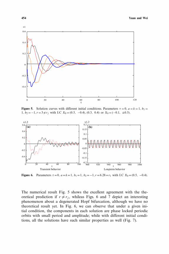
When we choose τ = 0, a = k = 1 and b1 = 1, b2 = −1 satisfying theassumptions in Theorem 2.9, we expect that all the solutions are stablewhen r �= rj ; while if r= rj , the degenerated Hopf bifurcation takes place.

454 Yuan and Wei

-0.4

-0.2

0

0.2

0.4

0.6

x1

0 20 40 60 80 100 120t

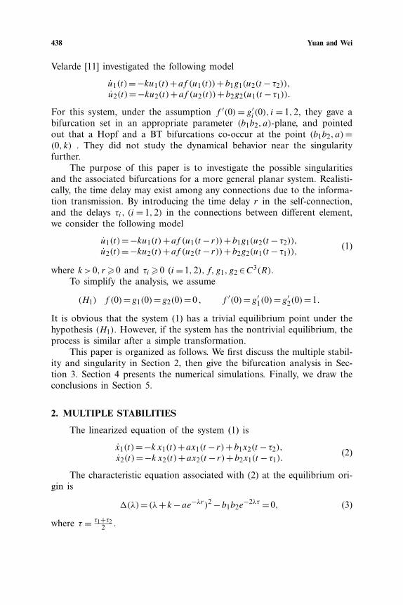
Figure 5. Solution curves with different initial conditions. Parameters τ = 0, a= k= 1, b1 =1, b2 =−1, r=3 �= rj with I.C X0 = (0.5, −0.4), (0.3, 0.4) or X0 = (−0.1, ±0.5).

-0.4

-0.2

0

0.2

0.4

0.6

0 20 40 60 80 100t

-0.2

-0.15

-0.1

-0.05

0

0.05

0.1

0.15

0.2x1,2

900 920 940 960 980 1000t

x1,2


(a) (b)

Figure 6. Parameters τ =0, a=k=1, b1 =1, b2 =−1, r=6.28= r1 with I.C X0 = (0.5, −0.4).

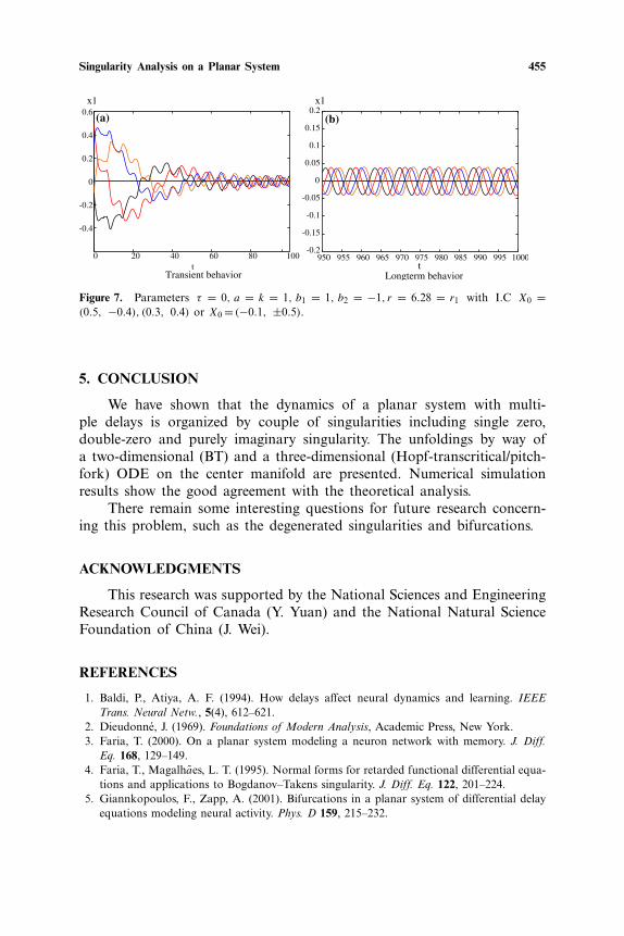
The numerical result Fig. 5 shows the excellent agreement with the the-oretical prediction if r �= rj , whileas Figs. 6 and 7 depict an interestingphenomenon about a degenerated Hopf bifurcation, although we have notheoretical result yet. In Fig. 6, we can observe that under a given ini-tial condition, the components in each solution are phase locked periodicorbits with small period and amplitude; while with different initial condi-tions, all the solutions have such similar properties as well (Fig. 7).


-0.4

-0.2

0

0.2

0.4

0.6x1

0 20 40 60 80 100t

-0.2

-0.15

-0.1

-0.05

0

0.05

0.1

0.15

0.2x1

950 955 960 965 970 975 980 985 990 995 1000t

(a) (b)


Figure 7. Parameters τ = 0, a = k = 1, b1 = 1, b2 = −1, r = 6.28 = r1 with I.C X0 =(0.5, −0.4), (0.3, 0.4) or X0 = (−0.1, ±0.5).

5. CONCLUSION

We have shown that the dynamics of a planar system with multi-ple delays is organized by couple of singularities including single zero,double-zero and purely imaginary singularity. The unfoldings by way ofa two-dimensional (BT) and a three-dimensional (Hopf-transcritical/pitch-fork) ODE on the center manifold are presented. Numerical simulationresults show the good agreement with the theoretical analysis.

There remain some interesting questions for future research concern-ing this problem, such as the degenerated singularities and bifurcations.

ACKNOWLEDGMENTS

This research was supported by the National Sciences and EngineeringResearch Council of Canada (Y. Yuan) and the National Natural ScienceFoundation of China (J. Wei).

REFERENCES

1. Baldi, P., Atiya, A. F. (1994). How delays affect neural dynamics and learning. IEEETrans. Neural Netw., 5(4), 612–621.

2. Dieudonne, J. (1969). Foundations of Modern Analysis, Academic Press, New York.3. Faria, T. (2000). On a planar system modeling a neuron network with memory. J. Diff.

Eq. 168, 129–149.4. Faria, T., Magalhaes, L. T. (1995). Normal forms for retarded functional differential equa-

tions and applications to Bogdanov–Takens singularity. J. Diff. Eq. 122, 201–224.5. Giannkopoulos, F., Zapp, A. (2001). Bifurcations in a planar system of differential delay

equations modeling neural activity. Phys. D 159, 215–232.

456 Yuan and Wei

6. Golubitsky, M., Langford, W. F. (1981). Classification and unfoldings of degenerate Hopfbifurcations. J. Diff. Eq. 41, 375–415.

7. Guckenheimer, J., Holmes, P. J. (1983). Nonlinear Oscillations, Dynamical Systems andBifurcations of Vector Fields, Springer-Verlag, New York.

8. Kertesz, V., Kooij, R. E. (1991). Degenerate Hopf bifurcation in two dimensions. Nonlin-ear Anal. Theory Appl. 17(3), 267–283.

9. Marcus, C. M., Waugh, F. R., Westervelt, R. M. (1991). Nonlinear Dynamics and Stabil-ity of Analog Neural Networks. Phys. D 51, 234–247.

10. Wei, J., Li, M. Y. (2004). Global existence of periodic solutions in a tri-neuron networkmodel with delays. Phys. D 198, 106–119.

11. Wei, J., Velarde, M. G. (2004). Bifurcation analysis and existence if periodic solutions in asimple neural network with delays. Chaos 14(3), 940–953.

12. Wu, J. (1998). Symmetric functional-differential equations and neural networks with mem-ory. Trans. Am. Math. Soc. 350(12), 4799–4838.

13. Yuan, Y., Campbell, S. A. (2004). Stability and synchronization of a ring of identical cellswith delayed coupling. J. Dyn. Diff. Eq. 16(1), 709–744.

14. Yuan, Y., Wei, J. (2006). Multiple bifurcation analysis in a neural network model withdelays. Int. J. Bifurcations Chaos 16(10), 1–10.

singularity analysis on a planar system with multiple delays

Documents