sinkholes and residential property prices: presence ......sinkholes and residential property prices:...
TRANSCRIPT

1
Sinkholes and Residential Property Prices: Presence, Proximity, and Density
by
Randy E. Dumm
William T. Hold Professor of Risk Management and Insurance
Dept. of Risk Management/Insurance, Real Estate, and Legal Studies
College of Business
Florida State University
Tallahassee, Florida 32306-1110
(850) 644-7880 (Phone)
(850) 644-4077 (Fax)
G. Stacy Sirmans Kenneth G. Bacheller Professor of Real Estate
Dept. of Risk Management/Insurance, Real Estate, and Legal Studies College of Business
Florida State University Tallahassee, Florida 32306-1110
(850) 644-7845 (Phone) (850) 644-4077 (Fax)
Greg T. Smersh Assistant Professor
Dept. of Finance College of Business
University of South Florida Tampa, Florida 33620
(813) 974-6239 (Phone) (813) 974-3084 (Fax)
October 2016

2
Sinkholes and Residential Property Prices: Presence, Proximity, and Density
Abstract
Spatial amenities, along with structural characteristics, affect residential property values. Although
the bundle of structural characteristics is typically the primary value determinant, studies have shown
that externalities and risk factors can adversely affect property values. This study uses residential
property sales data from 2000 to 2011 and sinkhole data from “sinkhole alley” in Florida to examine the
effect of sinkhole presence, proximity, and density on the sale price of residential real estate. Using a
hedonic pricing model, the results showed that properties located on a sinkhole sell for over nine percent
less, on average, relative to houses not located on a sinkhole. The results also showed the combined
effect of proximity to a sinkhole property and sinkhole density have a negative impact on selling price
but this effect is much stronger for sinkhole properties.

3
Sinkholes and Residential Property Prices: Presence, Proximity, and Density
1. Introduction
“A Florida couple is facing up to 20 years each in prison today for selling
their home without informing the buyers about an enormous sinkhole that
they knew was underneath it.” ABCNEWS.go.com, October 9, 2015
Location matters. Spatial amenities, along with structural characteristics, have definite effects on
residential property values. Although the bundle of structural characteristics is typically the primary
value determinant, studies have shown that externalities and other factors can affect property values.1
Externalities/factors such as golf course, ocean or lake view, proximity to a church, school quality, and
presence of trees have a positive effect on house prices while other externalities/factors such as
environmental contamination, landfills, proximity to power lines, flood plain, abandoned buildings, and
proximity to an interstate have a negative effect.2 In more recent studies, Dumm, Smersh, and Sirmans
(2016) show that waterfront properties command a price premium and Nyce, Dumm, Smersh, and
Sirmans (2015) show that homeowner’s insurance premiums have a negative effect on house prices.
This study uses Florida data to examine the effect of sinkholes on residential property values. The
study considers the presence, proximity, and density of sinkholes. As with other externalities, a sinkhole
may be both a property characteristic and a negative externality since it may affect the value of
surrounding properties. Along with hurricane and tropical storm risk, Florida ranks highest in the nation
for sinkhole risk. However, sinkhole location is less random and more localized than hurricanes and
earthquakes because their occurrence is more likely in areas where the land surface covers the types of
rock (limestone, carbonate rock, salt beds) that are naturally dissolved by groundwater.
Although states located primarily in the eastern U.S. are the most susceptible to sinkholes, other parts
of the country are not exempt. Sinkholes have appeared in Texas and Louisiana as a result of collapsing
salt domes. Western states such as Oklahoma, New Mexico, South Dakota, and Wyoming sit atop
gypsum, another type of soluble rock that can dissolve rapidly in water. Although Florida is especially
identified with sinkholes, if all underlying water soluble rock (karst, limestone, carbonate rock, gypsum,
and salt) across the U.S. is considered, forty percent of the ground cover of the United States is
susceptible to sinkholes.
Results show that sinkhole exposure adversely impacts on real estate valuation and the greatest
impact is for properties that contain a sinkhole. Additionally, proximity to and number of sinkholes off

4
the property also has an adverse effect on residential real estate selling prices. This effect is much smaller
than the main sinkhole effect and diminishes as the distance the property and sinkhole(s) increases.
2. Negative Externalities and Property Value
There is scant evidence explaining the relationship between house prices and sinkholes, either in
regard to sinkhole presence, proximity, or density. Only one previous study has examined the effect of
sinkholes on house prices. Fleury (2007) applies a hedonic pricing model to 1990 census data and the
Florida Geological Survey’s Sinkhole Database to examine the relationship between the
presence/density of sinkholes to the home values. Using data for the Tampa Bay, Florida area, he
estimates OLS and probit models with median home value by census block as the dependent variable.
He finds no significant effect of sinkhole presence or density on home values. He posits as possible
explanations: homebuyers may not be aware of sinkhole locations and that sinkholes may be viewed as
water features where homebuyers do not distinguish between man-made lakes and sinkholes. However,
another explanation may be that using census level data, such as median home value by census block,
obscures the true price variation across properties that are affected by sinkholes and those that aren’t.
For that reason, our study uses individual property transaction price data.3
Although the literature on sinkholes is lacking, there is ample literature showing the effects of
negative externalities on property values. Simons, Levin, and Sementelli (1997) examine the effect of
underground storage tanks on residential sales price. They examine three types of tanks: registered non-
leaking, nonregistered leaking tanks, and registered leaking tanks and find a 17% reduction in sale price.
In a following study, Simons, Bowen, and Sementelli (1999) examine the effects of leaking underground
storage tanks (LUSTs) from gas stations on residential and commercial property. Their results show a
14-16% reduction in sales price for residential properties a 28-42% reduction in sales price for
commercial properties. In a recent study of storage tanks, Zabel and Guignet (2012) examine the effect
of leaking underground storage tanks (LUSTs) on local soil and surface and groundwater. Their results
are interesting. They find that, although the typical LUST has no effect on surrounding property values,
more publicized and more severe sites caused a reduction in property values of more than ten percent.
Several studies have provided excellent literature reviews of the effects of environmental
contamination, air pollution, landfills, etc. Smith and Huang (1995) conduct meta-analysis of 37 air
pollution studies and find that a reduction in air pollution particulate increased property values. Farber
(1998) examines the literature on landfills, solid waste facilities, and superfund sites. Variables found
to affect property value included type of facility, distance, information relative to opening and closing

5
dates, thin markets, and employment effects. Boyle and Kiel (2001) review 30 papers for air pollution,
water quality, undesirable land uses, and pollution sources. They find that air quality features are
generally not known to buyers. They did find that water quality variables produced negative effects on
price and that undesirable land uses consistently produced negative effects on price. Jackson (2001)
examines 45 studies on environmental contamination and finds primarily negative effects on property
values. Simons and Saginor (2006) produce a meta-analysis of the effect of environmental
contaminations on residential real estate. They examine the effects of both environmental contamination
and positive amenities on proximate real estate property values in the U.S. The contaminated sites
include superfund sites, leaking underground storage tanks (LUSTs), landfills, pipeline ruptures, and
overhead transmission lines. They provide a literature review of 58 peer-reviewed papers on
contamination and 17 papers on positive amenities such as parks, beaches, etc. Their model examines
dollar property value loss and includes explanatory variables such as distance from source, type of
contamination, information, urban or rural environment, local and national market conditions,
remediation, etc. All of the contamination effects are negative.
One set of papers has examined the effect of flood hazard on residential property values. Skantz and
Strickland (1987) examine the effect of property values on first-time flooding. Interestingly, they find
that property values did not fall immediately after the flood. Instead, they find that house prices declined
about a year later when increased flood insurance premiums were capitalized into home prices. Harrison,
Smersh, and Schwartz (2001) examine changes in value for homes located within 100-year flood plains.
They find a negative effect on selling price for homes located within a flood zone. However, this
negative price effect is less than the present value of future flood insurance premiums. Bin and Polasky
(2004) estimate the effect of flood hazards on residential property value for properties that received
significant flooding from Hurricane Floyd in 1999. They find that properties located within a floodplain
experienced a decrease in property value and that the decrease is significantly larger after Hurricane
Floyd than before. Bin and Kruse (2006) examine the effects of flood hazard on residential property
values. Using digital flood maps coupled with residential property sales records, they find, on average,
a five to ten percent reduction in property values for properties located within a flood zone but not subject
to wave action. Interestingly, they find higher values for properties in flood plains subject to wave
action. They also find that price differentials were roughly equivalent to the capitalized value of flood
insurance premiums.
Examining the effect of earthquake risk, Murdoch, Singh, and Thayer (1993) find an area-wide
reduction in property values following the Loma Prieta (World Series) earthquake in the San Francisco

6
Bay area. Interestingly, they also find that apparently some homeowners considered other measures of
earthquake risk in their housing purchases, producing an obvious price gradient.4
3. What is a Sinkhole?
A sinkhole is a ground depression with no natural external surface drainage capability. Sinkholes
are most common in areas of “karst terrain”. The term “karst” is derived from the Slovenian word kras
which refers to the Kras region in Slovenia. The land areas of both Slovenia and Croatia (formerly
Yugoslavia) are major sinkhole areas.
A karst terrain is an area where the rocks below the land surface can naturally be dissolved by
groundwater circulating through them. Dissolvable types of rocks include salt beds and domes, gypsum,
limestone, and other carbonate rocks. As water soaks into the ground, these karst terrain rocks dissolve
creating underground caverns and spaces. At some point the underground space becomes too big for the
ground cover to support. The surface land collapses and a sinkhole results. About twenty percent of the
U.S. sits atop karst terrain. In fact, most states have some areas with karst terrain. The U.S. Geological
Survey map in Figure 1 shows the various underlying water-soluble rock across the United States and
thus the most sinkhole-prone areas. The shaded areas indicate various degrees of karst, limestone,
carbonate rock, and gypsum.
Although most sinkholes are “natural” phenomena, some sinkholes are correlated with events such
as flooding and land-use practices such as groundwater pumping and construction, which may lower the
water table. Real estate development such as buildings and parking lots can divert rainwater runoff and
result in concentrated weight that causes the ground cover to collapse. As Sinclair (1982) points out,
sinkholes may occur along certain joint patterns in the underlying bedrock. Pumping of large-capacity
wells along these joint patterns could increase the probability of sinkhole development.
[INSERT FIGURE 1 HERE]
In theory, the entire state of Florida is susceptible to sinkholes since it sits on porous carbonate rocks
such as limestone. Recognizing sinkhole risk, Florida law requires insurers to include in homeowners’
policies sinkhole activity coverage, for which insurers can charge an additional premium. Central
Florida’s geology makes that part of the state the most prone to sinkholes. Sinkholes are identified by
the Florida Geological Survey which collects geological data for the state.5
In addition to Florida, sinkholes are also becoming more common in other states. Along with natural
formations, sinkholes can also be precipitated by coal mines and aquifer systems. For example,

7
Pennsylvania is in the top seven states most at risk for sinkholes because it has coal mines and an
extensive underlay of limestone, especially through central Pennsylvania around the State College area
and from the Maryland state line up through Harrisburg and Lancaster. Also in Alabama, sinkholes
result from the underlying soluble carbonate rocks (especially north Alabama) and abandoned mines.
In the U.S., the most damage from sinkholes tends to occur in seven states: Florida, Texas, Alabama,
Missouri, Kentucky, Tennessee, and Pennsylvania. Sinkholes are not a problem unique to the United
States, however. Enormous sinkholes exist in Laos, New Guinea, and Venezuela. Sinkholes are also
found in Italy, South Africa, Australia, Croatia, China, Guatemala, Belize, and Mexico. Newton (1984)
provides a detailed analysis of sinkhole occurrence in the eastern United States. He identifies 850 sites
with an estimated 6,000 sinkholes in nineteen states. He confirms that the southern states most impacted
are Alabama, Florida, Georgia, and Tennessee with Pennsylvania as the most impacted northeastern state
and Missouri the most impacted Midwestern state. He estimates that the cost of damage and preventive
measures to minimize severity is about 170 million dollars.
4. Sinkhole Formation
Sinkholes are divided into three primary types: solution sinkholes, cover-collapse sinkholes, and
cover-subsidence sinkholes. With a solution sinkhole there is very little topsoil over the limestone or
other bedrock. Over time rain seeps into the crevices in the bedrock and dissolves it. This results in
the gradual formation of a depression. Cover-collapse sinkholes are the most dangerous because they
happen suddenly over a short period of time and can range in size. They are the result of erosion of
ground ground sediments forming an underground cavern. The continued erosion eventually causes
the surface layer to collapse and the sinkhole opens up suddenly. Cover-subsidence sinkholes are the
most common and form slowly over time as the ground gradually subsides or deflates. These occur as
the sand covering the bedrock slowly filters down in the bedrock crevices, eventually causing the land
surface to collapse. These sinkhole formations are less dramatic and less noticeable and may go
undetected for a time.
The U.S. Geological Survey (USGS) provides a mapping of the U.S. relative to sinkhole risk and
likely occurrence. The map in Figure 2 shows areas of possible underground cavern formation and
resulting sinkholes. The slash covered areas show the existence of evaporites (salt, gypsum, and
anhydrite) and carbonates (limestone and dolomite). About 35 to 40 percent of the U.S. is underlain
with evaporate rocks, although fortunately for many areas they are buried at great depths.
8
[INSERT FIGURE 2 HERE]
An interesting question is whether existing sinkholes are predictors of future sinkholes. Some studies
have attempted to predict the occurrence and distribution of sinkholes. Gao and Alexander (2003)
construct sinkhole probability maps for southeastern Minnesota. Based on distance to the nearest
sinkhole and sinkhole density, the authors create a decision tree to construct maps of relative sinkhole
risk. Their model successfully captures the details of the internal structure of high density areas but is
less successful in lower density areas. Upchurch and Littlefield (1988), using sinkhole data for
Hillsborough County, Florida, find that the distribution of ancient sinkholes in bare karst areas
successfully predicted the location of modern sinkholes. In areas of covered karst, the location of ancient
sinkholes did not predict modern sinkholes. The authors found, in bare karst areas, the sinkholes were
localized along major lineaments, consistent with Sinclair (1982).
Gutierrez and Lucha (2008) argue that two sinkhole components, the probability of occurrence and
the severity, must be considered in calculating sinkhole risk. Using a database for Spain that includes
location, chronology, size, and subsidence mechanisms, the authors find that trenching (clearing the
topsoil in order to observe the abutting relationships of faults and fractures) was useful predicting
sinkhole probability of occurrence and severity. Galve, Gutierrez, Lucha, Guerrero, Bonachea,
Remondo, and Cendrero (2009) examine sinkhole susceptibility and hazard by mapping three genetic
types of sinkholes. Susceptibility models were validated for each of the three types and were transformed
into a hazard map useful for developing preventive or corrective measures.
NASA has suggested that sinkholes may be spotted as they develop by using Interferometric
Synthetic Aperture Radar (InSAR). InSAR provides radar data from satellites and detects tiny
movements in the ground. For sinkholes that have some surface deformation prior to collapse, this could
be a monitoring system and provide some foresight in the case of some sinkholes. At present, there is
no plan to implement such a system country-wide in the U.S.
5. Florida is “Sinkhole Alley”
Although all states have some areas with karst terrain, unfortunately for Florida most of the state
consists of limestone karst terrain. Florida’s property and casualty insurers have seen an increase in
sinkhole claims over the last several years and sinkhole losses have risen. In a 2011 report, the Florida
Office of Insurance Regulation (OIR), the number of sinkhole claims increased from 2,360 in 2006 to

9
6,694 in 2010 (a total of 24,671 claims). 6 The approximate dollar amount of these claims was $1.4
billion.7
Within Florida, the ten most sinkhole-prone counties are:
1. Pasco 2. Hernando 3. Hillsborough 4. Marion 5. Pinellas 6. Citrus 7. Polk 8. Orange 9. Seminole 10. Lake
In Florida, three counties (Hernando, Hillsborough, and Pasco) are known as “sinkhole alley”. Per
the Florida Office of Insurance Regulation, over the period 2006 to 2010 two-thirds of the reported
damage claims came from these three counties. OIR reports that claims from sinkholes have increased
in recent years. In 2006, Florida saw 2,300 claims. By 2010 that number has risen to 6,700. Since there
is no geological explanation for the increase, the OIR suspects that some of the claims are questionable.
Insurance officials say claims are often paid without hard proof of damage.
Figure 3 shows the subsurface geology and sinkholes in Florida. Below are examples of the more
notorious sinkholes that have occurred. In late February 2013 a mouth 20 feet (6 meters) wide swallowed
37-year-old Jeff Bush as he slept in Seffner, Florida, inhaling his entire bedroom. Five others in the
house escaped without injury, including Jeremy Bush, who tried in vain to save his brother. (Jeremy
Berlin, National Geographic, August 13, 2013.) One of the most spectacular sinkholes occurred in 1981
in Winter Park, Florida. It was one city block in size and swallowed up a Porsche dealership. These are
the examples of the “classic” sinkholes that result in the complete collapse of the ground. They tend to
be different sinkholes than the sinkholes that we are examining in this study. Here, the assumption is
that the reported sinkhole is either located away from the house and the house has not been damaged, is
located near the house and has caused no or minimal damage, or is located near house and has been
repaired.
6. The Data
This study analyzes single-family detached home sales in Florida for Hillsborough county for the
period 2000 to 2011. Hillsborough County is approximately 1,000 square miles with a population of

10
roughly 1.3 million people, and therefore has a population density of around 1,300 persons per square
mile.
The data for this study are provided by the Hillsborough County Property Appraiser’s Offices which
provide data on property sales. This includes the property identification number, date of sale, dollar
amount of sale, section township range, and the type of legal instrument (i.e., Quit Claim, Warranty
Deed, etc.) recorded at the County Clerk’s office. This study includes only single-family detached
transactions. All sales in the final sample are verified as qualified sales or “arms-length” transactions.
All non-qualified sales (such as purchase by a relative, foreclosure, or any other non-arms-length
transaction) were deleted from the sample. Binary variables are used to represent the years 2001 to 2011,
with 2000 as the base year.
The data also include structural characteristics such as heated square footage, year built (used to
calculate age), number of baths flooring and lot size. Supplementary property characteristics such as
fireplace, swimming pool, central air conditioning and building construction quality are also available.
Some of these are converted to binary variables with a value of one to indicate the existence of the
specific characteristic or superior condition and zero otherwise. Structural characteristics were linked to
the sales database using the unique property identification number for each parcel. Some properties sold
more than once over the data period, but the year built variable was used to delete any homes that had
been rebuilt.
Hillsborough county provided parcel “shape files” which contain property parcel polygons in a
Geographic Information System (GIS) format. The parcel boundary and centroid (latitude / longitude
coordinate) are used to create additional variables. For example, a GIS spatial query was done to select
all the parcels that intersect the boundaries of the nearby water bodies over 10 acres in size to identify
those parcels as being on the water. GIS was also used to calculate the distance to Tampa Bay or the
Tampa central business district from each house.
Sections within a township/range are used to measure spatial dependence because they are commonly
recognized areas that (unlike census tracts or school districts) are not expected to be correlated with
house prices. A township is a measure of the distance north/south in units of six miles, while a range is
a measure of the distance east/west in units of six miles. A section is a one-square-mile block of land,
with 36 sections in a survey township. Data on the section / township / range for each property is
provided by the respective counties, and parcel centroids are used to identify location within these one-
square-mile areas. In this study, we use sections to adjust the standard errors.

11
Sinkholes are reported to and through the Florida Geological Survey (FGS) office. The FGS is the
premier state government institution in Florida specializing in geoscience research and assessments to
provide objective quality data and interpretations. They maintain and update GIS databases as part of
the statewide geomorphic mapping project. The FGS provides a mapping of the state relative to sinkhole
risk and likely occurrence. We utilized GIS to identify properties that contain reported sinkhole activity
and also to calculate the proximity of properties without sinkholes to the nearest property with a sinkhole.
GIS spatial queries were performed to calculate proximity within ¼-mile, between ¼-mile and ½-mile,
between ½-mile and 1-mile, between 1-mile and 2-miles, and farther than 2-miles for each property and
the number of sinkholes within each distance band.8
7. Methodology
Hedonic regression analysis is commonly used in real estate research to measure the marginal effects
of housing characteristics and other factors on house prices. A review by Sirmans, Macpherson and
Zietz (2005) of over 125 real estate studies that have used hedonic pricing models shows that many types
of variables, such as square feet, age, number of bedrooms and bathrooms, garage, pool, and fireplace,
have been included in these models. This study includes these variables and, additionally, variables to
measure the price effect of having a sinkhole on the property or a sinkhole located within a certain
proximity.
The general form of the hedonic pricing model is:
Pi = ƒ(Xi, Li, Ei)
where Pi is the log of the transaction price of house i, Xi is a vector of structural housing characteristics,
Li is a vector of location variables, and Ei is a vector of externalities affecting the transaction price. The
semi-log model is generally preferred since the coefficients provide semi-elasticities, i.e., the coefficients
are interpreted as the percentage change in price relative to a one-unit change in the explanatory variable
(Sirmans et al., 2005). The method typically used to measure the marginal effect of the explanatory
variables on the house price is OLS regression (Zietz et al., 2007) which minimizes the sum of the
squared residuals.
Our model includes variables representing several different aspects of sinkholes (presence,
proximity, and density) and binary variables for the years 2001 to 2011, with 2000 as the base year.
With these additional variables, the hedonic model can be written as:

12
Ln(SPj) = α0 + βi Xij + β Sinkholej + + β ShCtDj + β Timej + εi
where Ln(SP) is the natural log of the selling price, Xij is the matrix of explanatory variables, Sinkholej
is a binary variable with a value of one if a sinkhole is located on the property and zero otherwise,
The ShCtDj variables capture the number of sinkholes within a set distance from the property. As
such, they serve both as a measure of proximity and density.ShCt¼mj is the number of sinkholes within
a quarter-mile of the property, ShCt½mj is the number of sinkholes within a half-mile of the property,
ShCt1mj is the number of sinkholes within one mile of the property, and ShCt2mj is the number of
sinkholes within two miles of the property. These measures are cumulative in that each density measure
includes the sinkholes from the shorter distance density measure (e,g., the count for ShCt½m includes
the number of sinkholes reported for ShCt¼m). For properties with sinkholes on them, the ShCTDj
counts do not include that sinkhole. Timej is a vector of binary variables indicating the year of sale for
property j and εi is the error term.
The model is designed to measure two hypotheses. First, the presence of a sinkhole on the property
has a negative effect on the selling price of the property. According to this hypothesis the β on Sinkholej
< 0. Although Fleury (2007) shows no effect on sinkholes property values, a number of studies on
negative externalities provide evidence of a negative effect on property values (see, for example, Smith
and Huang (1995), Simons et al. (1997), Farber (1998), Simons et al. (1999), Jackson (2001), Simons
and Saginor (2006), and Zabel and Guighet (2012)).
The second hypothesis is that sinkhole density within a given radius of a property has a negative
effect on selling price. According to this second hypothesis the βs on the density variables (ShCt¼mj,
ShCt½mj, ShCt1mj, ShCt2mj) < 0 with a diminishing negative effect as distance increases. We expect to
see this relationship whether evaluating sinkhole density on a cumulative basis or within distance bands
(i.e., 1 mile) from the property. Although he found no significant statistical effect, Fleury (2007)
predicted that, based on economic theory, sinkhole density should have a negative effect on property
values. Regarding the effect of proximity to sinkholes, there is no published literature on the effect of
sinkhole proximity on property values but there are a number of studies showing a negative effect of
proximity to negative externalities. For example, Simons and Saginor (2006) show the negative effect
of environmental contamination on proximate real estate (see also Simons et al. (1997), Simons et al.
(1999), and Zabel and Guignet (2012)).

13
8. Results
The variables included in the regression model are defined in Table 1 and descriptive statistics are
provided in Tables 2 through 5. As shown in Table 2, houses that sold between 2000 and 2011 had an
average selling price of $213,564 and the average square footage was almost 1962 square feet. The
average age of the house was 19.5 years and the average lot size of just over ¼ acre. There were two
baths per house on average. Thirty percent of the houses had a swimming pool and 22% had a fireplace.
Almost all houses had central heating and cooling and about 47 percent had superior grade flooring.
Less than one percent of the homes were rated as superior construction.
[INSERT TABLE 1 HERE]
[INSERT TABLE 2 HERE]
Roughly 17 percent of the properties were waterfront properties while over 38% of the properties
were within ½ mile of a golf course. Both would be considered as desirable locational amentities. In
contrast, mobile homes and cemeteries would be considered less desirable. Seventeen percent of the
properties were located with ½ mile of a mobile home park while approximately two percent were
located near a cemetery. The variables, CBDDist measures the distance from a given property to the
City of Tampa’s central business district while BAYDist measures the distance to Tampa Bay. On
average, properties were located 10.8 miles from Tampa’s central business district and seven miles from
Tampa Bay. PopDensity captures the census track population densities for Hillsborough County. The
average population per census track was just over 3669 individuals with population density per census
track ranging from 1018 to 9851.
The primary focus of this paper is the impact of being located on a sinkhole and the combined
proximity and density effects of sinkholes external to the property on the selling price of residential real
estate. Sinkhole is a binary variable that has a value of one if the property contains a sinkhole and a
value of zero otherwise. To measure the effect of proximity and density, the number of sinkholes were
identified within ¼ miles, ½ miles, and 1 mile of the property. As noted above, each of these measures
is cumulative. Properties in the sample have an average density of 0.12 sinkholes within a quarter-mile
radius (minimum of zero, maximum of 25), 0.66 sinkholes within a half-mile radius (minimum of zero,
maximum of 38), 2.29 sinkholes within a one-mile radius (minimum of zero, maximum of 53), and 6.42
sinkholes within a two-mile radius (minimum of zero, maximum of 72).
[INSERT TABLE 3 HERE]

14
Table 3 provides for a comparison of means between properties with a sinkhole (as reported by the
Florida Geological Survey) and those that do not have sinkholes. The number of properties with a
sinkhole is very small (87 out of 212,947). It is interesting to note that sinkhole properties tend to have
significantly larger lot sizes. This may be because sinkhole locations are more rural but it also may
reflect how parcels with natural sinkholes on them were created. There is a lower frequency of sinkhole
properties in the high quality construction category than non-sinkhole properties. Additionally, sinkhole
properties are more likely to be newer, farther from Tampa Bay or the Tampa’s central business district,
and be near a golf course. The results in Table 3 also show that properties with sinkholes on them are
more likely to have more sinkholes near them. For example, the average number of sinkholes within a
mile of the property was over six times as large for properties that have sinkhole on them (16.2) than for
properties that do not (2.3). This effect increases as the distance from the property increases.
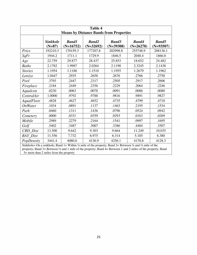
Table 4 provides more detail on the means for each of the distance bands related to sinkhole. Average
prices and square footage for properties with a sinkhole are higher than in Band 1 or Band 2. The average
age for properties with sinkholes (22.8 years) is substantially less than the properties in the immediate
vicinity (Bands 1-3). As noted above, the lot size for properties with a sinkhole is substantially larger
than is found in any of the distance bands.
Table 4 also provides information on property externalities. The percentage of properties with a
sinkhole that were near a mobile home community was higher than any other distance band (29.9%) but
over 54% of these properties were located in the vicinity of a golf cours. Given that sinkholes are
typically located off the coast, it is not surprising to observe that properties with a sinkhole were the
farthest from Tampa Bay (BAYDist= 13.5).
[INSERT TABLE 4 HERE]
The hedonic regression results for sinkhole presence and proximity are given in Table 5. The
Breusch-Pagan test was used to test for equal variances. Based on the test-statistic, the hypothesis of
equal variances was rejected, indicating the presence of heteroscedasticity. The standard errors were
clustered by the section variable (STR1). The adjusted R-squared is 0.77 and the F statistic is 567.25
indicating that the model performs adequately.
[INSERT TABLE 5 HERE]

15
Model 1 (Sinkhole Presence) includes control variables for housing characteristics, location
(proximity to externalities), binary variables controlling for time, and the presence of a sinkhole on the
property (Sinkhole). Building characteristics include square footage, age, lot size, swimming pool,
fireplace, quality of construction, floor quality, and central heating and cooling. All behave as expected.
Newer construction and waterfront have a positive effect on selling price. The binary variables for the
years show, as expected, that house prices increased steadily until 2006 after which prices steadily
declined until 2011.
The coefficient for the variable of primary interest, Sinkhole, is negative and significant, indicating
that the presence of a sinkhole on the property has a negative effect on the selling price of the property.
Properties located on a sinkhole sell for almost nine percent less, on average, than properties not located
on a sinkhole. Ideally, for sinkhole properties, we would like to know the relative proximity of the
sinkhole to the house or other structures but those data are not available.
Model 2 expands Model 1 to measure the price effect of nearby sinkhole density (¼ mile). The
results for the building characteristics, location, and years are consistent with those in Model 1. The
results also show the different effect that sinkhole density has on sinkhole properties and properties
without sinkhole. Using the average number of sinkholes for the ¼ mile band reported in Table 3 for
each group, the total sinkhole effect for sinkhole properties is a 9.1% reduction in price (-.0688+(-
.0070*3.26)= -.091). There was a negative density effect for properties not on sinkhole, but that effect
was small (-.01%).
In Model 3, sinkhole density is measured within ½ mile of the property. Here the results for the
housing and location variables are consistent with those reported in Model 1. The sinkhole variable
remains negative and significant (-.0653) and the aggregate sinkhole effect for properties on sinkhole is
a 9.3% reduction in price. As with Model 2, there is a small negative density effect for properties not
on sinkhole.
To further measure the combined proximity and density effect, Model 3 captures density in two
discrete 1 mile bands around the property. As noted above, the ½ mile sinkhole density measure used in
Model 3 is cumulative in that it includes the sinkholes located in the ¼ mile band. This is not the case
in Model 3. As with the prior models, the sinkhole coefficient remains negative and significant and both
band coefficients are also negative and significant with the outer 1 mile band coefficient (-.0011) smaller
than the inner band (-.0017). These results are consistent with the prior models in that the density effect
is much greater for sinkhole properties than for properties not on sinkhole (-10.7% versus -1%). The
results on the band coefficients also shows that the density effect decreases for properties with a sinkhole.

16
Model 5 contains only properties that do not have a sinkhole. The variables in this model are the
same as in Model 4 except for the sinkhole variable. Given the small number of sinkhole properties, we
would expect the results to be consistent with those reported in Model 4. The housing and location
results are consistent with the prior models and the 1 mile density band results are consistent with those
reported in Model 4.
The results in Table 5 provide strong support for our first hypothesis: that sinkhole properties sell
for significant discounts relative to properties without a sinkhole. The results in Table 5 provide support
our second hypothesis: that the combined effect of sinkhole proximity and density produces a negative
effect on selling price but that effect is much more pronounced for sinkhole properties.
9. Summary and Conclusions
This study has examined the effect of the presence of and the proximity to a sinkhole on house prices
using geo-coded Florida real estate home sales data for the period 2000 to 2011. Sinkholes may be both
a property characteristic and a negative externality since it can occur on the property itself and on
surrounding properties. Florida ranks highest in the nation for sinkhole risk since its primary land surface
covers rocks (such as limestone, carbonate rock, and salt beds) that can be naturally dissolved by
groundwater. Using a hedonic pricing model, the results showed that properties located on a sinkhole
sell for over nine percent less, on average, relative to houses not located on a sinkhole. The results also
showed the combined effect of proximity to a sinkhole property and sinkhole density have a negative
impact on selling price but this effect is much stronger for sinkhole properties.

17
References
Bin, O. and Kruse, J. (2006). "Real Estate Market Response to Coastal Flood Hazards." Nat. Hazards
Rev., 10.1061/(ASCE)1527-6988(2006)7:4(137), 137-144.
Bin, Okmyung and Stephen Polasky. "Effects of flood hazards on property values: evidence before and after Hurricane Floyd." Land Economics 80.4 (2004): 490-500.
David Harrison, Greg T. Smersh, and Arthur Schwartz (2001) Environmental Determinants of Housing Prices: The Impact of Flood Zone Status. Journal of Real Estate Research: 2001, Vol. 21, No. 1-2, pp. 3-20.
Dumm, R., G. Smersh, and G. S. Sirmans, “Price Variation in Waterfront Properties over the Economic
Cycle,” Journal of Real Estate Research, forthcoming 2015.
Fleury, S., "Are Home Values Affected by Sinkhole Proximity? Results of a Hedonic Price Model" The
Florida Geographer (2007): 72-84.
Galve, J. P., Gutiérrez, F., Lucha, P., Guerrero, J., Bonachea, J., Remondo, J., & Cendrero, A. (2009). Probabilistic sinkhole modelling for hazard assessment. Earth Surface Processes and Landforms, 34(3), 437-452.
Gao, Y., & Alexander, E. C. (2003, September). A Mathematical Model for a Map of Relative Sinkhole Risk in Fillmore County, Minnesota. In Sinkholes and the Engineering and Environmental Impacts
of Karst (2003) (pp. 439-449). ASCE.
Gutiérrez, F., Guerrero, J., & Lucha, P. (2008). Quantitative sinkhole hazard assessment. A case study from the Ebro Valley evaporite alluvial karst (NE Spain). Natural Hazards, 45(2), 211-233.
https://pubs.er.usgs.gov/publication/wri8150
https://www.nasa.gov/press/2014/march/nasa-radar-demonstrates-ability-to-foresee-
sinkholes/#.V5eJ5DVEpP0
J. C. Murdoch, H. Singh, and M. Thayer, “The Impact of Natural Hazards on Housing Values: The Loma Prieta Earthquake,” Real Estate Economics, 1993, 21:2, 167-184.
J. E. Zabel and D. Guignet, “A Hedonic Analysis of the Impact of LUST sites on House Prices,” Resource and Energy Economics Volume 34, Issue 4, November 2012, Pages 549–564
K. V. Smith and J. Huang, “Can Markets Value Air Quality? A Meta-Analysis of Hedonic Property
Value Models,” Journal of Political Economy, 1995, 103:1, 209-227
M. Boyle and K. Kiel, “A Survey of House Price Hedonic Studies of the Impact of Environmental
Externalities,” Journal of Real Estate Literature, 2001, 9:2, 116-144.
Newton, J. G. (1984). Natural and induced sinkhole development in the eastern United States. In Proceedings of the Third International Symposium on Land Subsidence, International Association
of Hydrological Sciences, Wallingford, UK (pp. 549-564).

18
Nyce, C., R. Dumm, G. Smersh, and G. S. Sirmans, “The Capitalization of Homeowners' Insurance
Premiums in House Prices,” Journal of Risk and Insurance, Vol. Vol. 82, No. 4, 2015.
R. A. Simons, A. M. Bowen, and A. J. Sementelli, “The Price and Liquidity Effects of UST Leaks
from Gas Stations and Adjacent Contaminated Property,” The Appraisal Journal, April 1999, 67,
186-194.
Robert A. Simons and Jesse D. Saginor, “A Meta-Analysis of the Effect of Environmental
Contamination and Positive Amenities on Residential Real Estate,” Journal of Real Estate
Research, 2006, 28:1, 71-104.
Robert Simons, William Levin, and Arthur Sementelli (1997) The Effect of Underground Storage
Tanks on Residential Property Values in Cuyahoga County, Ohio. Journal of Real Estate Research:
1997, Vol. 14, No. 1, pp. 29-42.
S. Farber, “Undesirable Facilities and Property Values: A Summary of Empirical Studies,” Ecological
Economics, 1998, 24, 1-14.
Seo, Y., and Simons, R.A., “The Effect of School Quality on Residential Sales Price,” Journal of Real
Estate Research, Vol. 31, No. 3, 2009 (pp. 307 – 327).
Sinclair, W. C. (1982). Sinkhole development resulting from ground-water withdrawal in the Tampa
area, Florida. US Geological Survey, Water Resources Division.
Sirmans, G. S., D. A. Macpherson, and E. Zietz. The Composition of Hedonic Pricing Models. Journal
of Real Estate Literature, 2005, 13:1, 1-44.
T. Jackson, “The Effects of Environmental Contamination of Real Estate: A Literature Review,”
Journal of Real Estate Literature, 2001, 9:2, 93-116.
Terrance Skantz and Thomas Strickland (1987) House Prices and a Flood Event: An Empirical Investigation of Market Efficiency. Journal of Real Estate Research: 1987, Vol. 2, No. 2, pp. 75-83.
Upchurch, S. B., & Littlefield Jr, J. R. (1988). Evaluation of data for sinkhole-development risk models. Environmental Geology and Water Sciences, 12(2), 135-140.
Stephanie Pappas “What are Sinkholes?” Live Science, March 15, 2014. http://www.livescience.com/44123-what-are-sinkholes.html
Anthony F. Radazzo, “Are There Different Types of Sinkholes?” October 15, 2015. http://www.geohazardsinc.com/why-do-sinkholes-form-in-florida/
Endnotes
1. In their 2005 review of 125 hedonic pricing models studies (examining over 150 variables),
Sirmans, Macpherson, and Zietz show that 17 of the top twenty variables appearing in these studies are housing characteristics.

19
2. For a comprehensive review of hedonic pricing models, see Sirmans, Macpherson, and Zietz (2005). They review 125 studies that have used hedonic pricing models in residential real estate. They examine over 150 variables.
3. One important point that Fluery (2007) makes is that sinkholes serve as a signal to the public of possible environmental effects, most of which are negative. The most extreme of these is the possible loss of property and/or life. There may also be negative effects of being located within proximity of a sinkhole(s) since this would presumably increase the possibility of a sinkhole developing on your property. A possible positive effect would be that the sinkhole may have an aesthetic appeal, for example has the appearance of a natural or man-made lake.
4. Although some people have expressed concerns about the relationship between fracking and sinkholes, there seems to be a dearth of literature connecting the two. For example, writing in a Politics and International Relations blog published on December 10, 2014, Charlie Provah indicates that fracking produces concerns not only about chemical contamination and air pollution but also about sinkholes
5. The geomorphology of Florida is unique because most of the state is not a sediment ramp off the piedmont or continent to the Atlantic Ocean or the Gulf of Mexico. The Floridian section is part of an enormous carbonate bank, called the Florida Platform, which has existed since at least the Cretaceous Period. Residing entirely within the Coastal Plain, Florida is part of an enormous carbonate bank, called the Florida Platform, covered by a thin layer of younger quartz sand and clay sediments. It is these carbonate rocks which are, in part, responsible for many of the karst features common to Florida, such as springs and sinkholes.
6. RiskMeter.com from CDS Business Mapping provides a sinkhole database and sinkhole clearinghouse which contains more than 12,000 sinkholes. It is used by underwriters and agents to determine proximity to natural hazards, including sinkholes.
7. Sources: Florida Department of Environmental Protection and Florida Senate report.
8. In general, a seller has a duty to disclose any material defect that may affect the property value thus proximity to a sinkhole(s) is important. Florida statute requires that sellers and lessors disclose “known” sinkhole activity in an area.

20
Figure 1. Areas in the U.S. Susceptible to Sinkhole Formation
MAP COURTESY U.S. GEOLOGICAL SURVEY
Figure 2. United States Map of Sinkhole Risk

21
Figure 3. Florida Sinkholes

22
Table 1
Variable Definitions
Variable Definition
Ln(sp) Log of sale price ln(sp) = dependent variable
SqFt The square footage of the house
Age Age of house at the time of sale
Baths Number of bathrooms
Stories Number of stories
Lotsize The size of the lot in acres.
Pool Binary variable with a value of one if the house has a pool, zero otherwise
Fireplace Binary variable with a value of one if the house has a fireplace, zero otherwise
Aqualcon Binary variable with a value of one for superior, excellent or above average construction rating, zero otherwise
Aqualroof Binary variable of one for superior roof cover, zero otherwise
CentralAir Binary variable of one if the house has central air, zero otherwise
AqualFloor Binary variable of one if the flooring is tile, hardwood or marble, zero otherwise
OnWater Binary variable of one for property on the water, zero otherwise
Park Binary variable of one for property located within one-half mile of a recreation park,
zero otherwise
Cemetery Binary variable of one for property located with one-half mile of a cemetery, zero
otherwise
Mobile Binary variable of one for property located with one-half mile of a mobile home park,
zero otherwise
Golf Binary variable for property located within 100 yards of a golf course, zero otherwise
CBD_Dist Distance from the property to the central business district
BAY_Dist Distance from the property to the bay district
PopDensity Census track population density
Sinkhole Binary variable with a value of one if there is a sinkhole on the property, zero
otherwise
ShCt¼m The number of sinkholes within a quarter-mile of the property
ShCt½m The number of sinkholes within a half-mile of the property
ShCt1m The number of sinkholes within one mile of the property
ShCT1_2m The number of sinkholes between one and two miles of the property
Y2001 –
Y2011
Time trend variables for the years 2001 through 2012 (Y2000 is the omitted year)

23
Table 2
Descriptive Statistics
(N=212947)
Variable Mean Std. Dev. Min Max
Price 213564 167235 10500 6500000
SqFt 1961.96 784.04 770 9921
Age 19.5324 21.4155 0 125
Baths 2.2389 .7437 1 9.5
Stories 1.2220 .4192 1 5
Lotsize .2758 .4530 .01 39.69
Pool .2959 .4564 0 1
Fireplace .2186 .4133 0 1
Aqualcon .0062 .0782 0 1
AqualFloor .4668 .4989 0 1
CentralAir .9868 .1140 0 1
OnWater .1696 .3752 0 1
Park .0841 .2775 0 1
Cemetery .0196 .1387 0 1
Mobile .1720 .3774 0 1
Golf .3867 .4870 0 1
CBD_Dist 10.7798 4.5570 .71 26.59
BAY_Dist 7.0426 4.7549 0 26.06
PopDensity 3979.1 2158.59 1018 9851
Sinkhole .0004 .0202 0 1
ShCt¼m .1911 .8758 0 25
ShCt½m .6629 1.9721 0 38
ShCt1m 2.2920 4.7541 0 53
ShCt1_2m 6.4203 9.6718 0 72
Y2001 .0878 .2831 0 1
Y2002 .0924 .2896 0 1
Y2003 .1023 .3030 0 1
Y2004 .1121 .3155 0 1
Y2005 .1300 .3363 0 1
Y2006 .0913 .2880 0 1
Y2007 .0499 .2176 0 1
Y2008 .0438 .2047 0 1
Y2009 .0516 .2212 0 1
Y2010 .0482 .2141 0 1
Y2011 .0512 .2204 0 1

24
Table 3
Mean Comparison: Property On versus Off Sinkhole
Variable
Off Sinkhole
(N=212860)
On Sinkhole
(N=87) DIFF SIG
Price 213572.9 192210.3 21362.5
SqFt 1961.97 1944.23 17.7
Age 19.53 22.78 -3.23 **
Baths 2.23 2.17 .06
Stories 1.22 1.19 .03
Lotsize .275 1.044 .769 **
Pool .296 .379 -.083 *
Fireplace .219 .218 .001
Aqualcon .006 .022 -.016
AqualFloor .467 .482 -.015
CentralAir .986 1.00 -.014
OnWater .169 .103 .066 **
Park .084 .046 .038 **
Cemetery .019 0.00 .019
Mobile .172 .299 -.127 ***
Golf .387 .540 -.153 ***
CBD_Dist 10.78 13.50 -2.72 ***
BAY_Dist 7.04 11.56 -4.52 ***
PopDensity 3971.1 3441.4 528.7 *** ShCt¼m .190 3.126 -2.936 *** ShCt½m .660 6.597 -5.937 *** ShCt1m 2.286 16.172 -13.886 *** ShCt2m 8.702 33.758 -25.056 *** *significant at the 10% level; **significant at the 5% level; ***significant at the 1% level.
25
Table 4
Means by Distance Bands from Properties
Sinkhole
(N=87)
Band1
(N=16752)
Band2
(N=32692)
Band3
(N=39308)
Band4
(N=26278)
Band5
(N=93507)
Price 192210.3 170159.3 177207.8 202998.8 255748.9 208136.1
SqFt 1944.2 1711.1 1729.9 1846.5 2048.4 1866.0
Age 22.759 29.877 28.437 25.853 18.652 24.482
Baths 2.1782 1.9987 2.0264 2.1198 2.3245 2.1438
Stories 1.1954 1.1186 1.1510 1.1955 1.2679 1.1962
Lotsize 1.0447 .2935 .2658 .2676 .2766 .2758
Pool .3793 .2447 .2317 .2505 .2917 .2606
Fireplace .2184 .2449 .2356 .2229 .2064 .2246
Aqualcon .0230 .0063 .0078 .0091 .0086 .0080
CentralAir 1.0000 .9792 .9788 .9816 .9891 .9827
AqualFloor .4828 .4627 .4652 .4735 .4799 .4710
OnWater .1034 .0891 .1137 .1463 .2195 .1534
Park .0460 .1311 .1436 .0796 .0524 .0942
Cemetery .0000 .0331 .0359 .0293 .0163 .0269
Mobile .2989 .2279 .2164 .1541 .0997 .1695
Golf .5402 .3487 .3007 .3386 .4404 .3507
CBD_Dist 13.500 9.642 9.303 9.664 11.249 10.035
BAY_Dist 11.556 7.732 6.975 6.314 5.105 6.380
PopDensity 3441.4 4080.6 4136.9 4256.1 4170.8 4128.3
Sinkhole= On a sinkhole; Band 1= Within ¼ mile of the property; Band 2= Between ¼ and ½ mile of the property; Band 3= Between ½ and 1 mile of the property; Band 4= Between 1 and 2 miles of the property; Band 5= more than 2 miles from the property

26
Table 5
Regression Output
Model 1 Model 2 Model 3 Model 4 Model 5
SqFt .0004*** .0004*** .0004*** .0004*** .0004***
(.0000) (.0000) (.0000) (.0000) (.0000)
Age -.0028*** -.0028*** -.0028*** -.0028*** -.0028***
-(.0005) -(.0005) -(.0005) -(.0005) -(.0005)
Baths .0839*** .0838*** .0839*** .0839*** .0840***
-(.0069) -(.0069) -(.0070) -(.0069) -(.0069)
Stories -.0440*** -.0440*** -.0441*** -.0443*** -.0443***
-(.0122) -(.0122) -(.0122) -(.0121) -(.0121)
Lotsize .0547*** .0548*** .0548*** .0556*** .0568***
-(.0085) -(.0085) -(.0085) -(.0086) -(.0088)
Pool .1259*** .1260*** .1262*** .1273*** .1272***
-(.0084) -(.0084) -(.0084) -(.0083) -(.0083)
Fireplace .1018*** .1022*** .1025*** .1036*** .1034***
-(.0117) -(.0118) -(.0118) -(.0119) -(.0119)
Aqualcon .2444*** .2442*** .2441*** .2428*** .2433***
-(.0220) -(.0220) -(.0220) -(.0218) -(.0219)
AqualFloor .0654*** .0651*** .0648*** .0641*** .0641***
-(.0048) -(.0048) -(.0048) -(.0047) -(.0047)
CentralAir .1746*** .1751*** .1754*** .1765*** .1766***
-(.0159) -(.0159) -(.0159) -(.0158) -(.0158)
OnWater .0677*** .0677*** .0678*** .0677*** .0676***
-(.0114) -(.0114) -(.0114) -(.0114) -(.0114)
Park -.0600** -.0597** -.0589** -.0563** -.0563**
-(.0262) -(.0262) -(.0262) -(.0262) -(.0262)
Cemetery -.0662 -.0668 -.0673 -.0682 -.0682
-(.0554) -(.0553) -(.0552) -(.0551) -(.0551)
Mobile -.0363** -.0360** -.0353** -.0321* -.0321*
-(.0165) -(.0165) -(.0166) -(.0165) -(.0165)
Golf .0916*** .0920*** .0923*** .0947*** .0948***
-(.0206) -(.0206) -(.0206) -(.0208) -(.0208)
CBD_Dist -.0035 -.0035 -.0036 -.0044 -.0044
-(.0030) -(.0030) -(.0030) -(.0030) -(.0030)
BAY_Dist -.0115*** -.0113*** -.0110*** -.0100*** -.0100***
-.0024 -.0024 -.0023 -.0023 -.0023
PopDensity .0000 .0000 .0000 .0000 .0000
(.0000) (.0000) (.0000) (.0000) (.0000)
Sinkhole -.0883** -.0688* -.0653* -.0692*
-(.0382) -(.0375) -(.0375) -(.0371)
ShCt¼m -.0070***
-(.0027)

27
ShCt½m -.0042**
-(.0017)
ShCt1m -.0017** -.0017**
-(.0008) -(.0008)
ShCt1_2m -.0011* -.0011*
-(.0006) -(.0006)
Y2001 .0261*** .0262*** .0261*** .0261*** .0260***
-(.0067) -(.0067) -(.0067) -(.0067) -(.0067)
Y2002 .0928*** .0927*** .0927*** .0929*** .0929***
-(.0074) -(.0074) -(.0073) -(.0073) -(.0073)
Y2003 .1761*** .1759*** .1759*** .1758*** .1757***
-(.0086) -(.0086) -(.0086) -(.0085) -(.0086)
Y2004 .3070*** .3069*** .3069*** .3069*** .3069***
-(.0092) -(.0092) -(.0092) -(.0092) -(.0092)
Y2005 .5171*** .5170*** .5171*** .5172*** .5171***
-(.0100) -(.0100) -(.0100) -(.0100) -(.0100)
Y2006 .6643*** .6644*** .6647*** .6642*** .6642***
-(.0104) -(.0104) -(.0104) -(.0104) -(.0104)
Y2007 .5973*** .5974*** .5977*** .5968*** .5967***
-(.0115) -(.0115) -(.0115) -(.0115) -(.0115)
Y2008 .3895*** .3895*** .3896*** .3891*** .3891***
-(.0098) -(.0098) -(.0098) -(.0098) -(.0098)
Y2009 .1161*** .1160*** .1160*** .1155*** .1155***
-(.0109) -(.0110) -(.0109) -(.0109) -(.0109)
Y2010 .1321*** .1319*** .1318*** .1317*** .1316***
-(.0079) -(.0078) -(.0078) -(.0078) -(.0078)
Y2011 .0629*** .0628*** .0629*** .0628*** .0628***
-(.0095) -(.0095) -(.0095) -(.0095) -(.0095)
_cons 1.7162*** 1.7169*** 1.7177*** 1.7251*** 1.7252***
-(.0426) -(.0426) -(.0426) -(.0425) -(.0425) N 212947 212947 212947 212947 212860
R2 .7727 .7728 .7729 .7732 .7732 *- Significant at 10%; **- Significant at 5%; ***- Significant at 1%
Betas in parentheses