sirius - physics and astronomy at tamupeople.physics.tamu.edu/depoy/astr314/notes/lecture7.pdf ·...
TRANSCRIPT
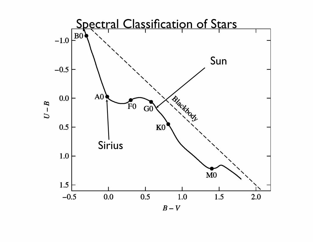
Sirius
Sun
Spectral Classification of Stars
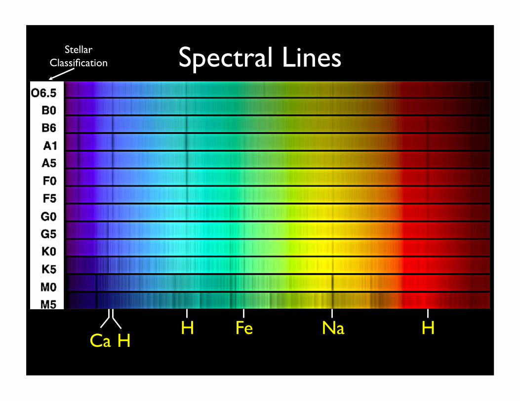
Spectral Lines
Na H H
H Ca
Fe
Stellar Classification
Spectral Classification of Stars
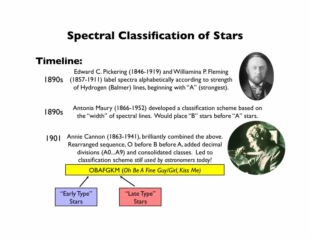
Edward C. Pickering (1846-1919) and Williamina P. Fleming (1857-1911) label spectra alphabetically according to strength
of Hydrogen (Balmer) lines, beginning with “A” (strongest).
Timeline:
1890s
1890s Antonia Maury (1866-1952) developed a classification scheme based on the “width” of spectral lines. Would place “B” stars before “A” stars.
1901 Annie Cannon (1863-1941), brilliantly combined the above. Rearranged sequence, O before B before A, added decimal
divisions (A0...A9) and consolidated classes. Led to classification scheme still used by astronomers today!
OBAFGKM (Oh Be A Fine Guy/Girl, Kiss Me)
“Early Type” Stars
“Late Type” Stars
Spectral Classification of Stars Timeline:
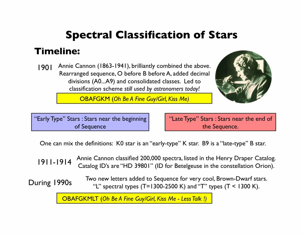
1901 Annie Cannon (1863-1941), brilliantly combined the above. Rearranged sequence, O before B before A, added decimal
divisions (A0...A9) and consolidated classes. Led to classification scheme still used by astronomers today!
OBAFGKM (Oh Be A Fine Guy/Girl, Kiss Me)
“Early Type” Stars : Stars near the beginning of Sequence
“Late Type” Stars : Stars near the end of the Sequence.
One can mix the definitions: K0 star is an “early-type” K star. B9 is a “late-type” B star.
Annie Cannon classified 200,000 spectra, listed in the Henry Draper Catalog. Catalog ID’s are “HD 39801” (ID for Betelgeuse in the constellation Orion). 1911-1914
During 1990s Two new letters added to Sequence for very cool, Brown-Dwarf stars. “L” spectral types (T=1300-2500 K) and “T” types (T < 1300 K).
OBAFGKMLT (Oh Be A Fine Guy/Girl, Kiss Me - Less Talk !)
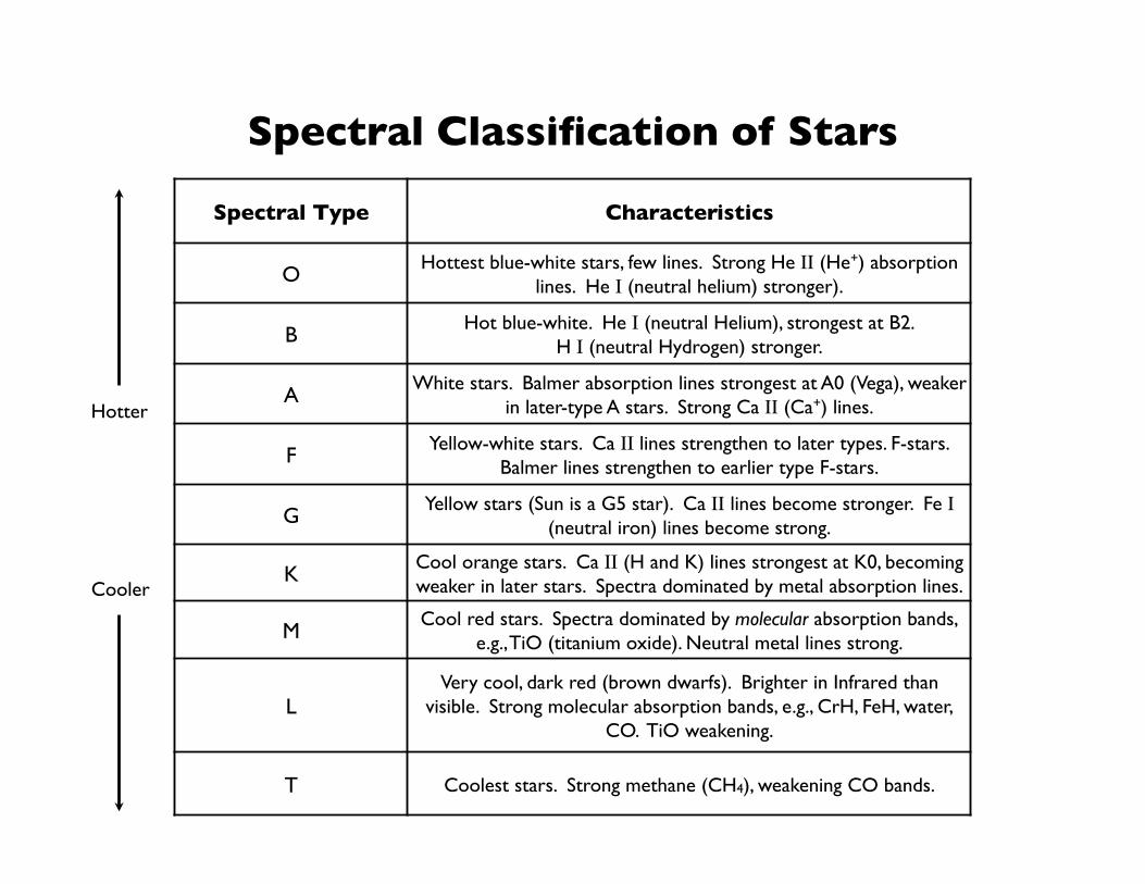
Spectral Classification of Stars
Spectral Type Characteristics
O Hottest blue-white stars, few lines. Strong He II (He+) absorption
lines. He I (neutral helium) stronger).
B Hot blue-white. He I (neutral Helium), strongest at B2.
H I (neutral Hydrogen) stronger.
A White stars. Balmer absorption lines strongest at A0 (Vega), weaker
in later-type A stars. Strong Ca II (Ca+) lines.
F Yellow-white stars. Ca II lines strengthen to later types. F-stars.
Balmer lines strengthen to earlier type F-stars.
G Yellow stars (Sun is a G5 star). Ca II lines become stronger. Fe I
(neutral iron) lines become strong.
K Cool orange stars. Ca II (H and K) lines strongest at K0, becoming weaker in later stars. Spectra dominated by metal absorption lines.
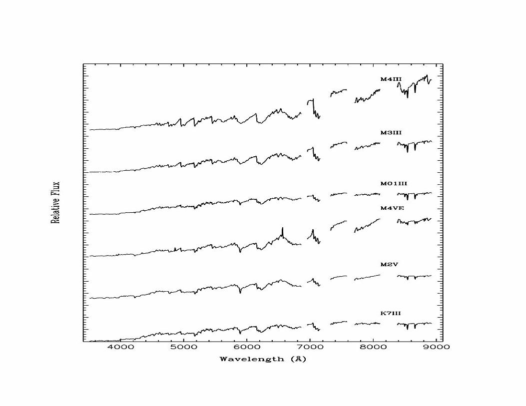
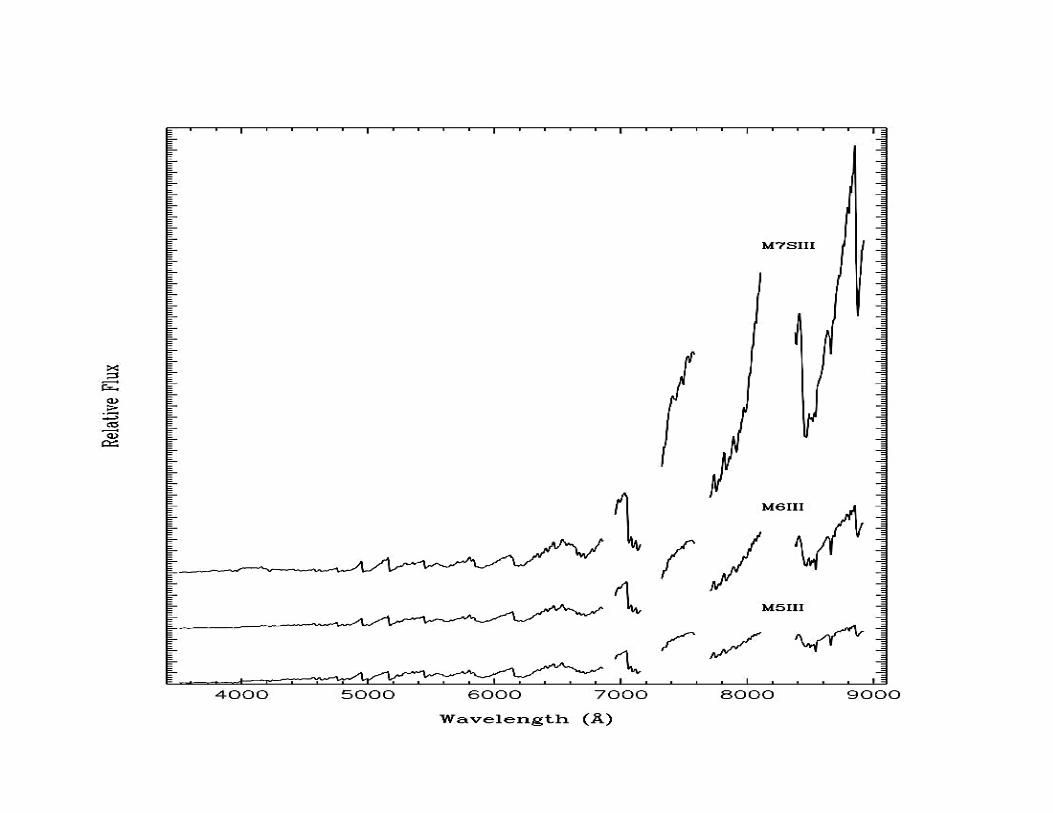
M Cool red stars. Spectra dominated by molecular absorption bands,
e.g., TiO (titanium oxide). Neutral metal lines strong.
L Very cool, dark red (brown dwarfs). Brighter in Infrared than
visible. Strong molecular absorption bands, e.g., CrH, FeH, water, CO. TiO weakening.
T Coolest stars. Strong methane (CH4), weakening CO bands.
Hotter
Cooler
Spectral Classification of Stars
Spectral Classification of Stars
Spectral Classification of Stars
Spectral Classification of Stars
Spectral Classification of Stars
Spectral Classification of Stars Physical Description
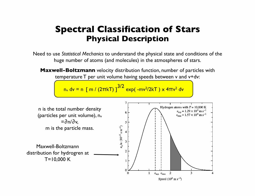
Need to use Statistical Mechanics to understand the physical state and conditions of the huge number of atoms (and molecules) in the atmospheres of stars.
Maxwell-Boltzmann velocity distribution function, number of particles with temperature T per unit volume having speeds between v and v+dv:
nv dv = n exp( -mv2/2kT ) x 4πv2 dv [ m / (2πkT) ] 3/2
n is the total number density (particles per unit volume), nv
=∂n/∂v, m is the particle mass.
Maxwell-Boltzmann distribution for hydrogren at
T=10,000 K
Spectral Classification of Stars Physical Description
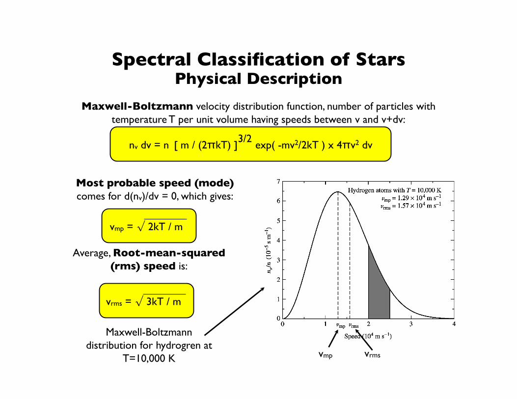
Maxwell-Boltzmann velocity distribution function, number of particles with temperature T per unit volume having speeds between v and v+dv:
nv dv = n exp( -mv2/2kT ) x 4πv2 dv [ m / (2πkT) ] 3/2
Most probable speed (mode) comes for d(nv)/dv = 0, which gives:
vmp = √ 2kT / m
Average, Root-mean-squared (rms) speed is:
vrms = √ 3kT / m
Maxwell-Boltzmann distribution for hydrogren at
T=10,000 K vrms vmp
Spectral Classification of Stars Physical Description
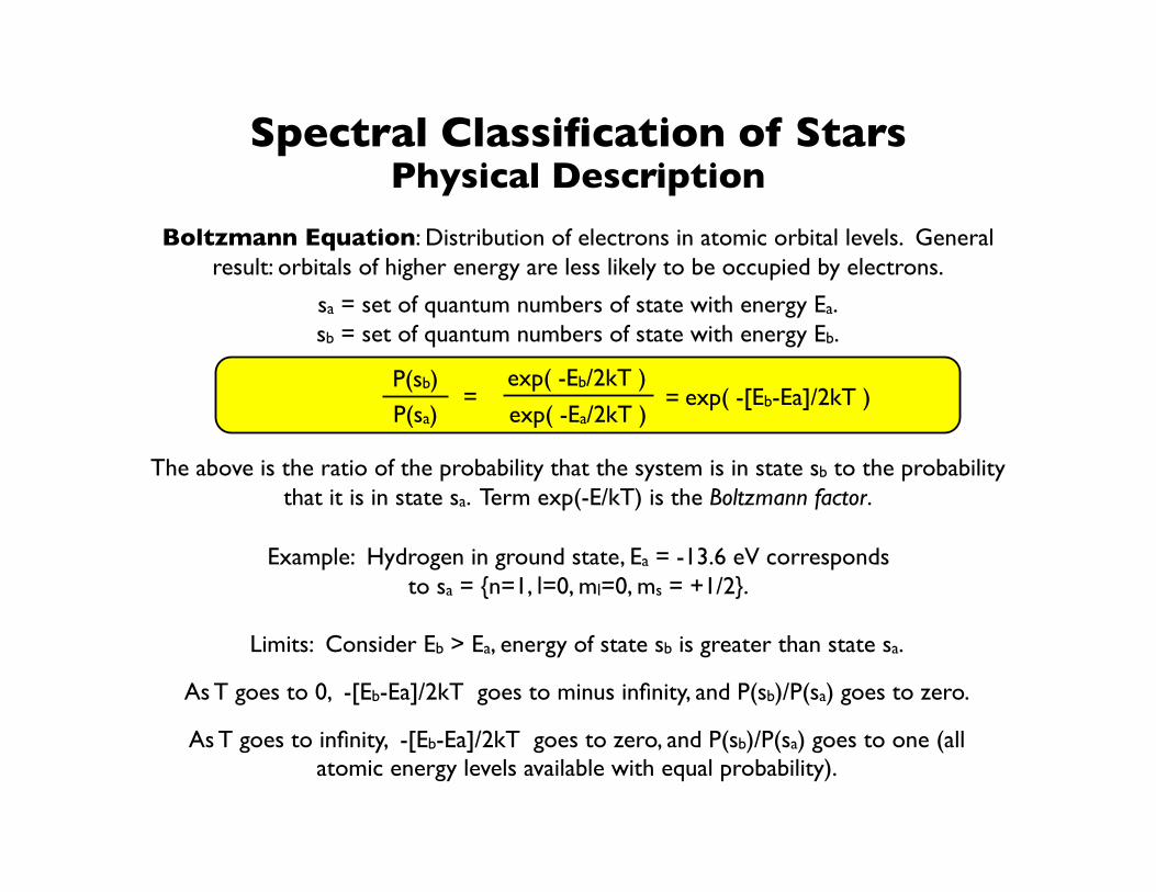
Boltzmann Equation: Distribution of electrons in atomic orbital levels. General result: orbitals of higher energy are less likely to be occupied by electrons.
P(sb) exp( -Eb/2kT ) =
P(sa) exp( -Ea/2kT )
sa = set of quantum numbers of state with energy Ea. sb = set of quantum numbers of state with energy Eb.
The above is the ratio of the probability that the system is in state sb to the probability that it is in state sa. Term exp(-E/kT) is the Boltzmann factor.
= exp( -[Eb-Ea]/2kT )
Limits: Consider Eb > Ea, energy of state sb is greater than state sa.
As T goes to 0, -[Eb-Ea]/2kT goes to minus infinity, and P(sb)/P(sa) goes to zero.
As T goes to infinity, -[Eb-Ea]/2kT goes to zero, and P(sb)/P(sa) goes to one (all atomic energy levels available with equal probability).
Example: Hydrogen in ground state, Ea = -13.6 eV corresponds to sa = {n=1, l=0, ml=0, ms = +1/2}.
Spectral Classification of Stars Physical Description
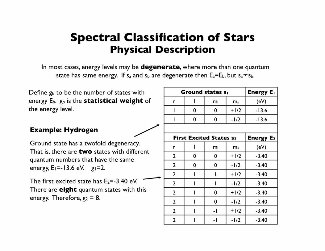
In most cases, energy levels may be degenerate, where more than one quantum state has same energy. If sa and sb are degenerate then Ea=Eb, but sa≠sb.
Example: Hydrogen
Ground state has a twofold degeneracy. That is, there are two states with different quantum numbers that have the same energy, E1=-13.6 eV. g1=2.
The first excited state has E2=-3.40 eV. There are eight quantum states with this energy. Therefore, g2 = 8.
Ground states s1 Energy E1
n l ml ms (eV)
1 0 0 +1/2 -13.6
1 0 0 -1/2 -13.6
First Excited States s2 Energy E2
n l ml ms (eV)
2 0 0 +1/2 -3.40
2 0 0 -1/2 -3.40
2 1 1 +1/2 -3.40
2 1 1 -1/2 -3.40
2 1 0 +1/2 -3.40
2 1 0 -1/2 -3.40
2 1 -1 +1/2 -3.40
2 1 -1 -1/2 -3.40
Define gb to be the number of states with energy Eb. gb is the statistical weight of the energy level.
Spectral Classification of Stars Physical Description
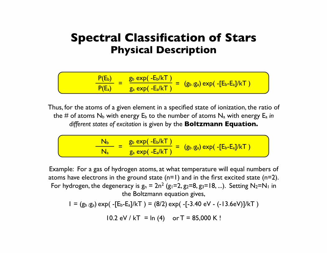
P(Eb) gb exp( -Eb/kT ) =
P(Ea) ga exp( -Ea/kT ) = (gb /ga) exp( -[Eb-Ea]/kT )
Thus, for the atoms of a given element in a specified state of ionization, the ratio of the # of atoms Nb with energy Eb to the number of atoms Na with energy Ea in
different states of excitation is given by the Boltzmann Equation.
Nb gb exp( -Eb/kT ) =
Na ga exp( -Ea/kT ) = (gb /ga) exp( -[Eb-Ea]/kT )
Example: For a gas of hydrogen atoms, at what temperature will equal numbers of atoms have electrons in the ground state (n=1) and in the first excited state (n=2). For hydrogen, the degeneracy is gn = 2n2 (g1=2, g2=8, g3=18, ...). Setting N2=N1 in
the Boltzmann equation gives,
1 = (gb /ga) exp( -[Eb-Ea]/kT ) = (8/2) exp( -[-3.40 eV - (-13.6eV)]/kT )
10.2 eV / kT = ln (4) or T = 85,000 K !
Spectral Classification of Stars Physical Description
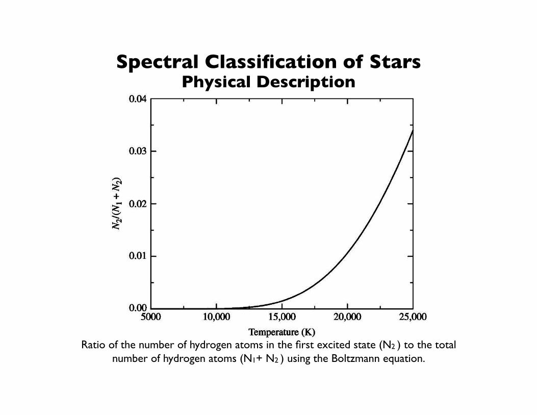
Ratio of the number of hydrogen atoms in the first excited state (N2 ) to the total number of hydrogen atoms (N1+ N2 ) using the Boltzmann equation.
Spectral Classification of Stars Physical Description
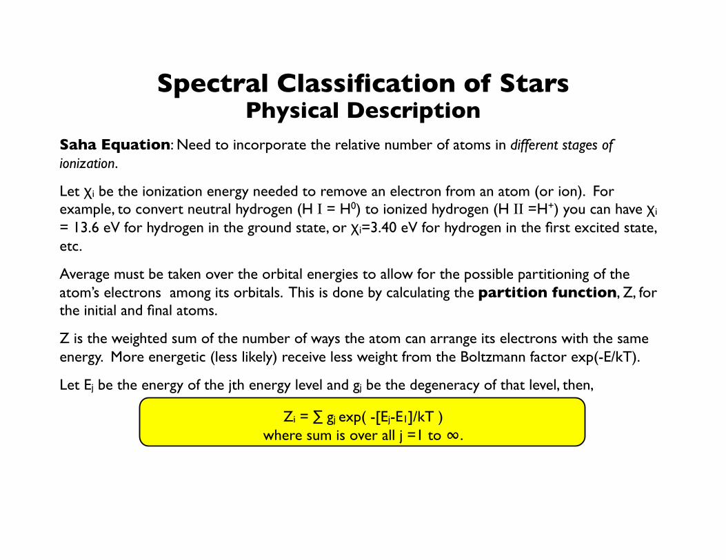
Saha Equation: Need to incorporate the relative number of atoms in different stages of ionization.
Let χi be the ionization energy needed to remove an electron from an atom (or ion). For example, to convert neutral hydrogen (H I = H0) to ionized hydrogen (H II =H+) you can have χi = 13.6 eV for hydrogen in the ground state, or χi=3.40 eV for hydrogen in the first excited state, etc.
Average must be taken over the orbital energies to allow for the possible partitioning of the atom’s electrons among its orbitals. This is done by calculating the partition function, Z, for the initial and final atoms.
Z is the weighted sum of the number of ways the atom can arrange its electrons with the same energy. More energetic (less likely) receive less weight from the Boltzmann factor exp(-E/kT).
Let Ej be the energy of the jth energy level and gj be the degeneracy of that level, then,
Zi = ∑ gj exp( -[Ej-E1]/kT ) where sum is over all j =1 to ∞.
Spectral Classification of Stars Physical Description
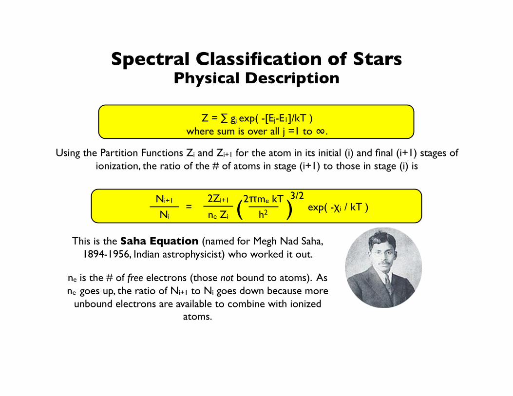
This is the Saha Equation (named for Megh Nad Saha, 1894-1956, Indian astrophysicist) who worked it out.
Z = ∑ gj exp( -[Ej-E1]/kT ) where sum is over all j =1 to ∞.
Using the Partition Functions Zi and Zi+1 for the atom in its initial (i) and final (i+1) stages of ionization, the ratio of the # of atoms in stage (i+1) to those in stage (i) is
Ni+1 2Zi+1 =
Ni ne Zi ( exp( -χi / kT ) ) 2πme kT
h2
3/2
ne is the # of free electrons (those not bound to atoms). As ne goes up, the ratio of Ni+1 to Ni goes down because more
unbound electrons are available to combine with ionized atoms.
Spectral Classification of Stars Physical Description
Spectral Classification of Stars Physical Description
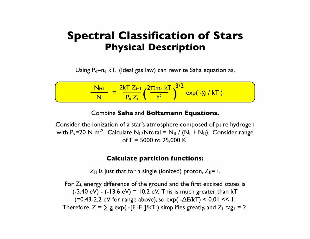
Using Pe=ne kT, (Ideal gas law) can rewrite Saha equation as,
Ni+1 2kT Zi+1 =
Ni Pe Zi ( exp( -χi / kT ) ) 2πme kT
h2
3/2
Combine Saha and Boltzmann Equations.
Consider the ionization of a star’s atmosphere composed of pure hydrogen with Pe=20 N m-2. Calculate NII/Ntotal = NII / (NI + NII). Consider range
of T = 5000 to 25,000 K.
Calculate partition functions:
ZII is just that for a single (ionized) proton, ZII=1.
For ZI, energy difference of the ground and the first excited states is (-3.40 eV) - (-13.6 eV) = 10.2 eV. This is much greater than kT (=0.43-2.2 eV for range above), so exp( -ΔE/kT) < 0.01 << 1.
Therefore, Z = ∑ gj exp( -[Ej-E1]/kT ) simplifies greatly, and ZI ≈g1 = 2.
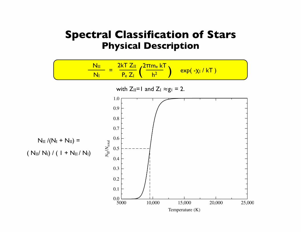
Spectral Classification of Stars Physical Description
NII 2kT ZII =
NI Pe ZI ( exp( -χI / kT ) ) 2πme kT
h2
with ZII=1 and ZI ≈g1 = 2.
NII /(NI + NII) =
( NII/ NI) / ( 1 + NII / NI)
Spectral Classification of Stars Physical Description
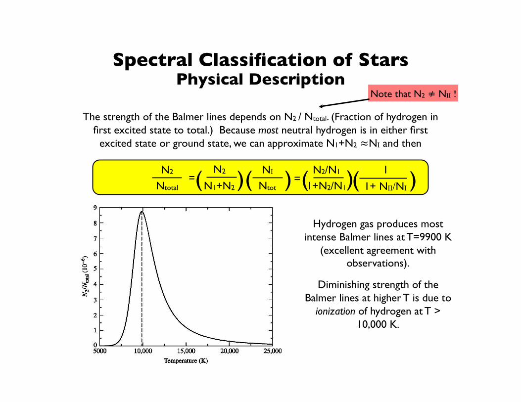
N2 N2 =
Ntotal N1+N2 ( ) NI
Ntot
The strength of the Balmer lines depends on N2 / Ntotal. (Fraction of hydrogen in first excited state to total.) Because most neutral hydrogen is in either first
excited state or ground state, we can approximate N1+N2 ≈NI and then
Note that N2 ≠ NII !
) ( = N2/N1
1+N2/N1 ( 1
1+ NII/NI ) ( )
Hydrogen gas produces most intense Balmer lines at T=9900 K
(excellent agreement with observations).
Diminishing strength of the Balmer lines at higher T is due to
ionization of hydrogen at T > 10,000 K.
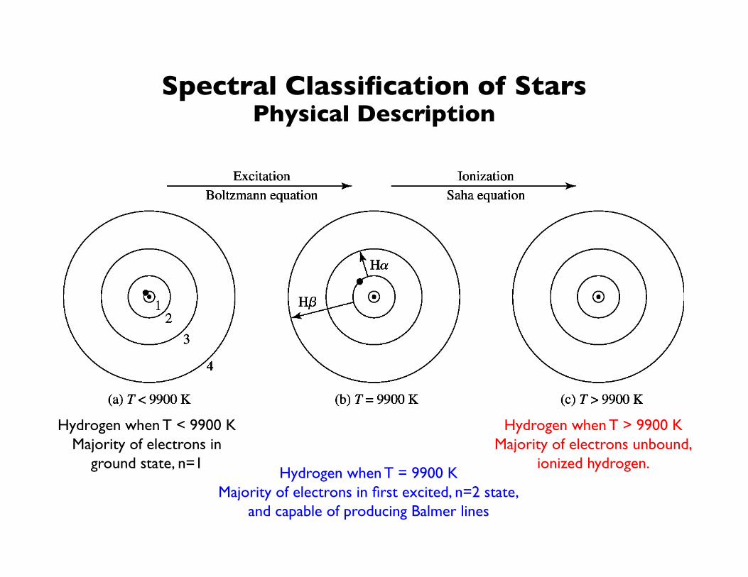
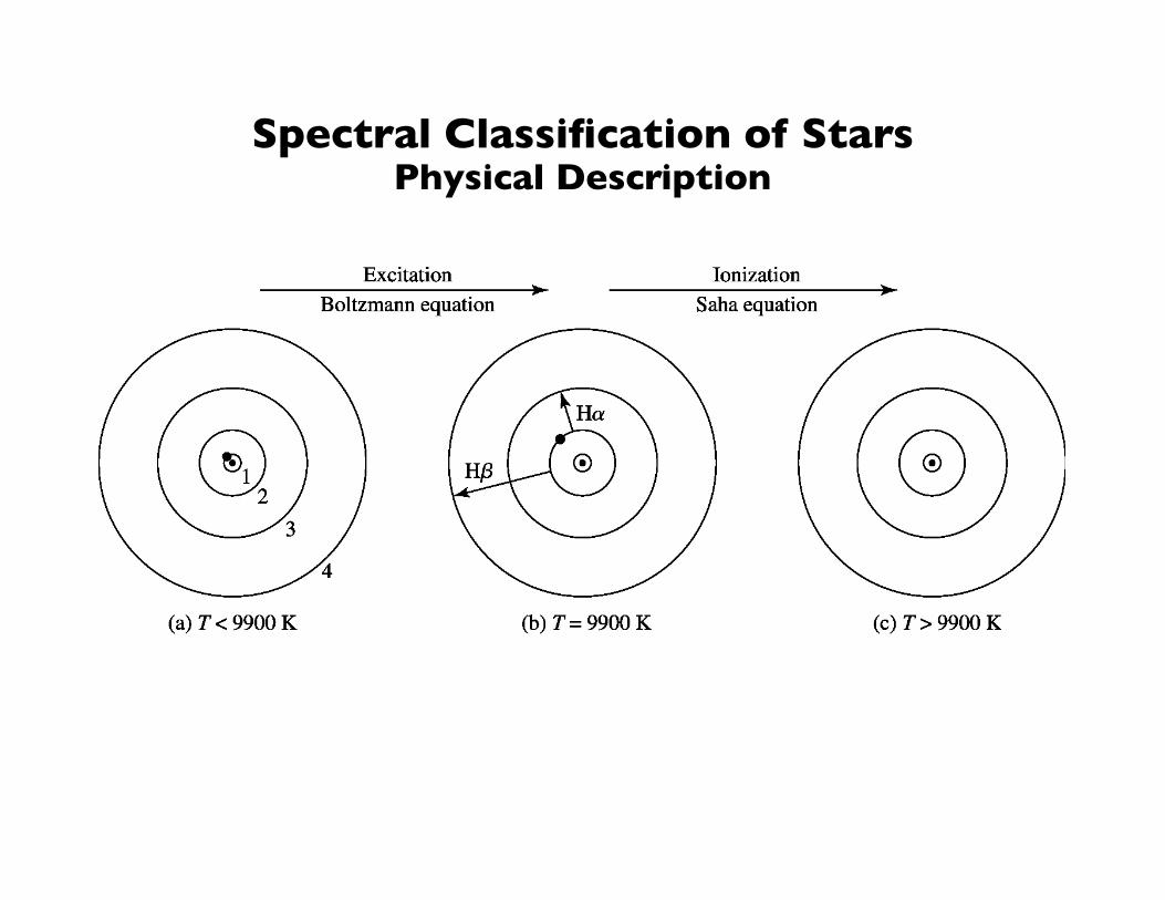
Spectral Classification of Stars Physical Description
Hydrogen when T < 9900 K Majority of electrons in
ground state, n=1 Hydrogen when T = 9900 K
Majority of electrons in first excited, n=2 state, and capable of producing Balmer lines
Hydrogen when T > 9900 K Majority of electrons unbound,
ionized hydrogen.
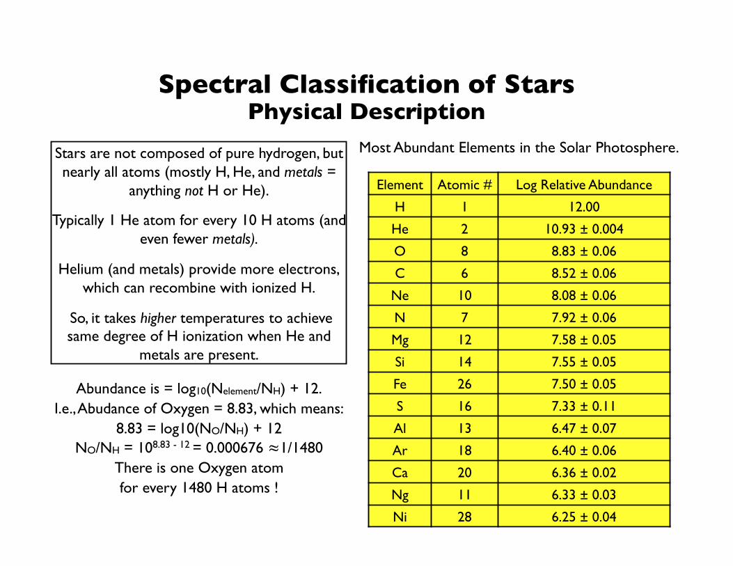
Most Abundant Elements in the Solar Photosphere.
Spectral Classification of Stars Physical Description
Stars are not composed of pure hydrogen, but nearly all atoms (mostly H, He, and metals =
anything not H or He).
Typically 1 He atom for every 10 H atoms (and even fewer metals).
Helium (and metals) provide more electrons, which can recombine with ionized H.
So, it takes higher temperatures to achieve same degree of H ionization when He and
metals are present.
Element Atomic # Log Relative Abundance
H 1 12.00
He 2 10.93 ± 0.004
O 8 8.83 ± 0.06
C 6 8.52 ± 0.06
Ne 10 8.08 ± 0.06
N 7 7.92 ± 0.06
Mg 12 7.58 ± 0.05
Si 14 7.55 ± 0.05
Fe 26 7.50 ± 0.05
S 16 7.33 ± 0.11
Al 13 6.47 ± 0.07
Ar 18 6.40 ± 0.06
Ca 20 6.36 ± 0.02
Ng 11 6.33 ± 0.03
Ni 28 6.25 ± 0.04
Abundance is = log10(Nelement/NH) + 12. I.e., Abudance of Oxygen = 8.83, which means:
8.83 = log10(NO/NH) + 12 NO/NH = 108.83 - 12 = 0.000676 ≈1/1480
There is one Oxygen atom for every 1480 H atoms !

Spectral Classification of Stars Physical Description
Consider a Sun-like star with T=5777 K and 500,000 H atoms for each Calcium (Ca) atom with Pe = 1.5 N m-2. Calculate relative strength of Balmer and singly
ionized Ca (Ca II).
NII 2kT Zi+1 =
NI Pe Zi ( exp( -χi / kT ) = 7.7 x 10-5 =1 / 13,000 ) 2πme kT
h2
3/2
Hydrogen: Saha equation gives ratio of ionized to neutral atoms.
1 ionized hydrogen ion (H II) for every 13,000 neutral hydrogen atoms
Hydrogen: Boltzmann equation gives ratio of atoms in first excited state to ground state.
N2 =
N1 (g2/g1) exp( -[E2-E1]/kT ) = 5.06 x 10-9 = 1 / 198,000,000
1 hydrogen ion in the first excited state for every 198 million hydrogen atoms in the ground state.
Spectral Classification of Stars Physical Description
NII 2kT ZII =
NI Pe ZI ( exp( -χI / kT ) = 918. ) 2πme kT
h2
3/2
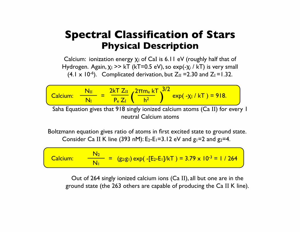
Calcium: ionization energy χI of CaI is 6.11 eV (roughly half that of Hydrogen. Again, χI >> kT (kT=0.5 eV), so exp(-χi / kT) is very small
(4.1 x 10⁻⁶). Complicated derivation, but ZII =2.30 and ZI =1.32.
Saha Equation gives that 918 singly ionized calcium atoms (Ca II) for every 1 neutral Calcium atoms
Boltzmann equation gives ratio of atoms in first excited state to ground state. Consider Ca II K line (393 nM): E2-E1=3.12 eV and g1=2 and g2=4.
N2 =
N1 (g2/g1) exp( -[E2-E1]/kT ) = 3.79 x 10-3 = 1 / 264
Out of 264 singly ionized calcium ions (Ca II), all but one are in the ground state (the 263 others are capable of producing the Ca II K line).
Calcium:
Calcium:
Spectral Classification of Stars Physical Description
N1 N1 ≈
Ntotal N1+N2 ( ) NII
Ntot ) ( = 1
1+N2/N1 ( NII/NI 1+ NII/NI ) ( ) ( )
CaII CaII Ca CaII Ca
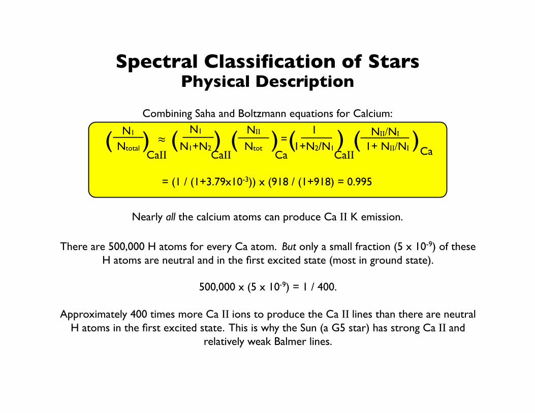
= (1 / (1+3.79x10⁻³)) x (918 / (1+918) = 0.995
Combining Saha and Boltzmann equations for Calcium:
There are 500,000 H atoms for every Ca atom. But only a small fraction (5 x 10⁻⁹) of these H atoms are neutral and in the first excited state (most in ground state).
500,000 x (5 x 10-9) = 1 / 400.
Approximately 400 times more Ca II ions to produce the Ca II lines than there are neutral H atoms in the first excited state. This is why the Sun (a G5 star) has strong Ca II and
relatively weak Balmer lines.
Nearly all the calcium atoms can produce Ca II K emission.
Spectral Classification of Stars Physical Description
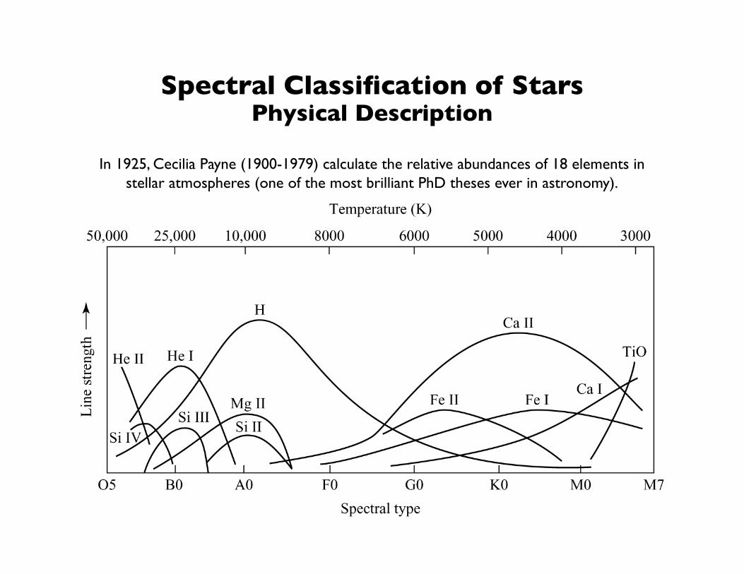
In 1925, Cecilia Payne (1900-1979) calculate the relative abundances of 18 elements in stellar atmospheres (one of the most brilliant PhD theses ever in astronomy).
Spectral Classification of Stars
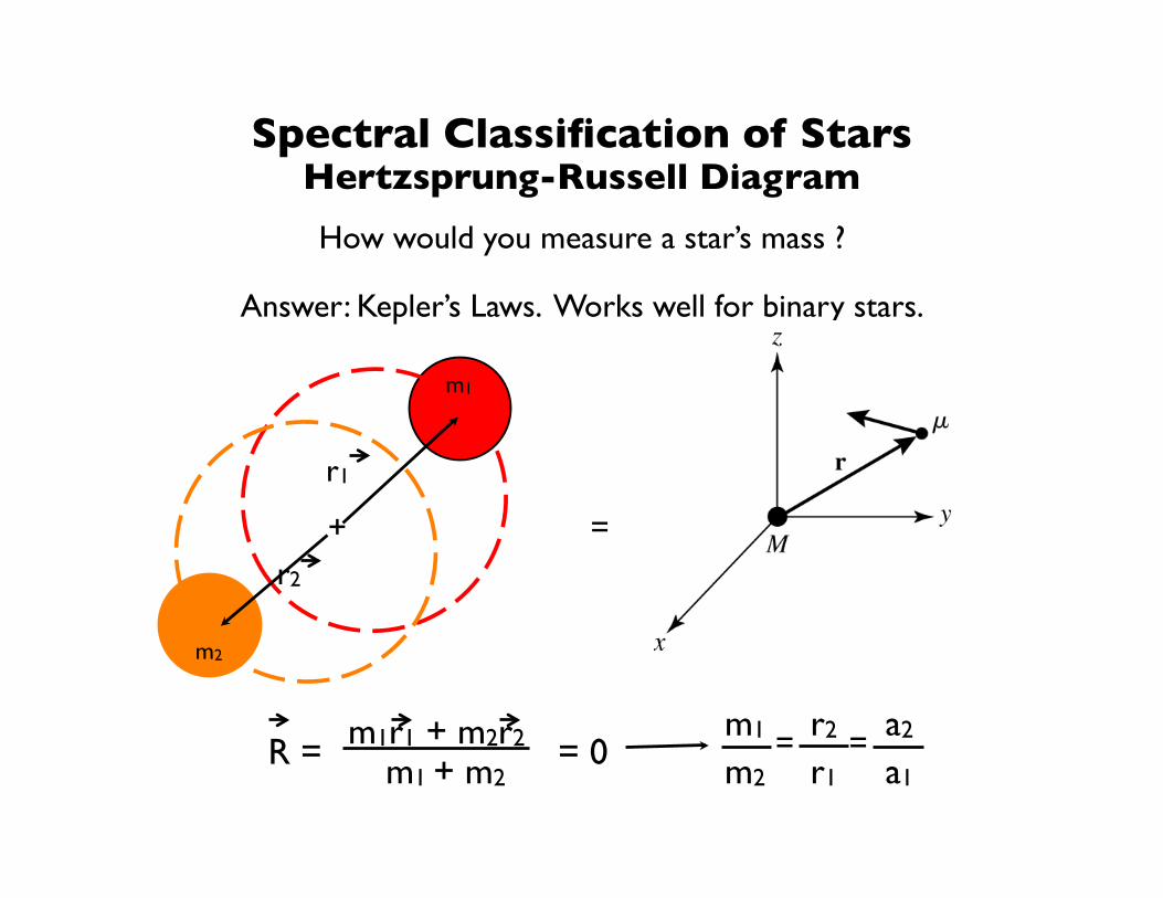
How would you measure a star’s mass ?
Hertzsprung-Russell Diagram
Spectral Classification of Stars
How would you measure a star’s mass ?
+
Answer: Kepler’s Laws. Works well for binary stars.
=
r1
r2
m1
m2
m1r1 + m2r2 R = m1 + m2 = 0
m1
m2
r2
r1
a2
a1 = =
Hertzsprung-Russell Diagram
Animations of binary Stars:
http://astro.ph.unimelb.edu.au/software/binary/binary.htm
http://abyss.uoregon.edu/~js/applets/eclipse/eclipse.htm
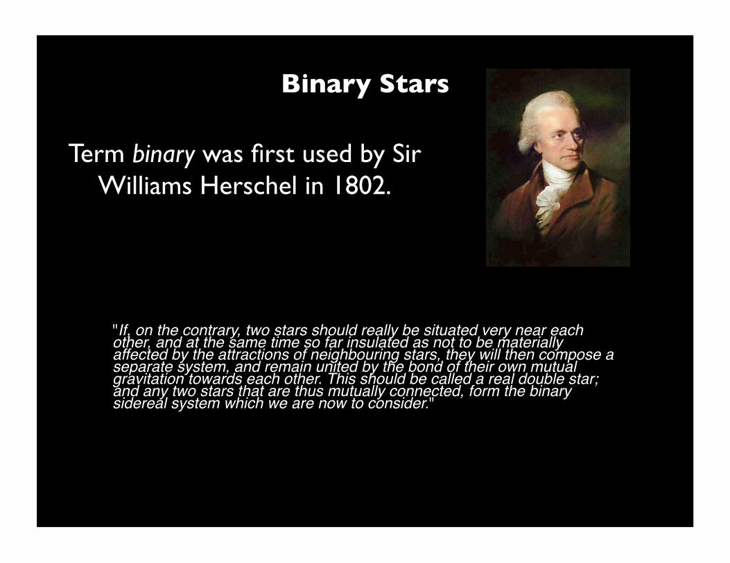
Binary Stars
Term binary was first used by Sir Williams Herschel in 1802.
"If, on the contrary, two stars should really be situated very near each other, and at the same time so far insulated as not to be materially affected by the attractions of neighbouring stars, they will then compose a separate system, and remain united by the bond of their own mutual gravitation towards each other. This should be called a real double star; and any two stars that are thus mutually connected, form the binary sidereal system which we are now to consider."
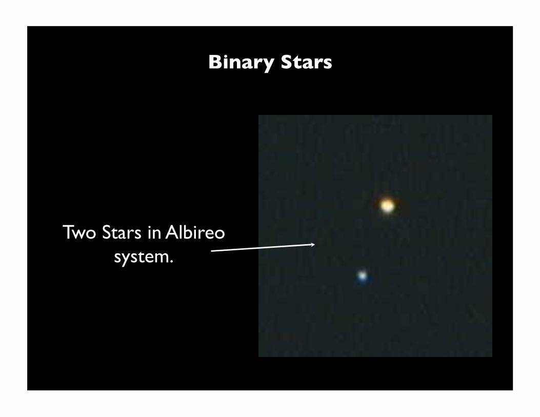
Binary Stars
Two Stars in Albireo system.
Binary Stars
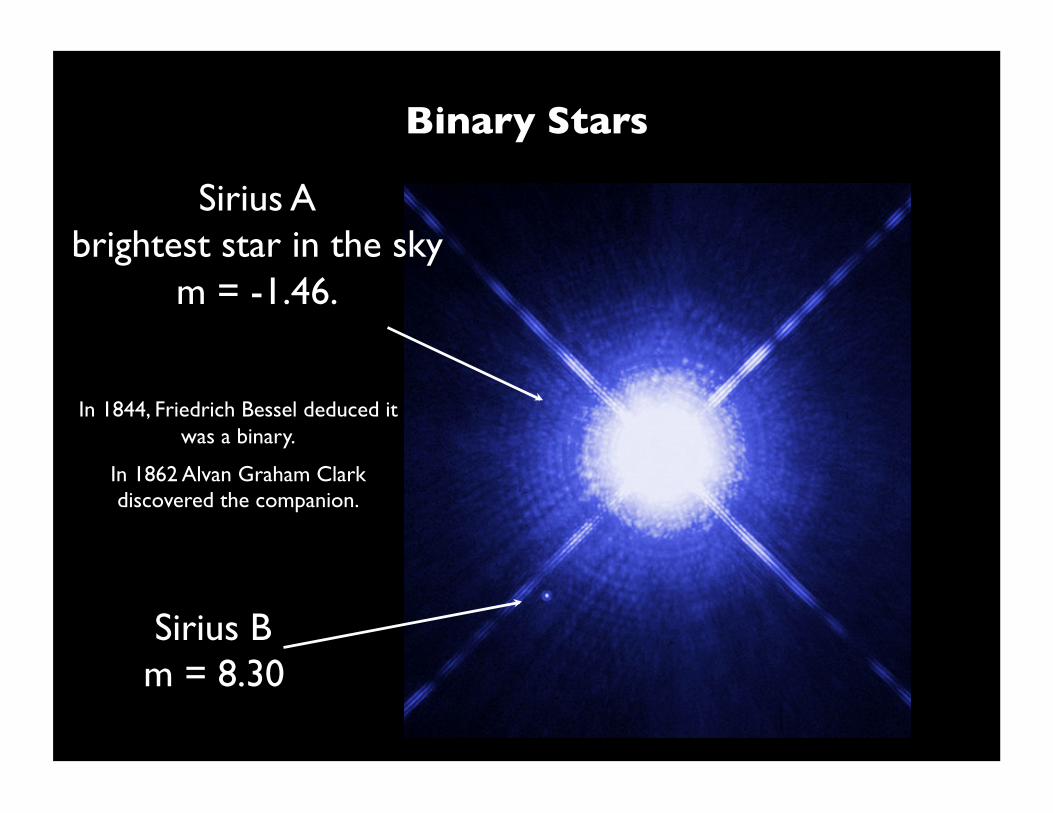
Sirius A brightest star in the sky
m = -1.46.
Sirius B m = 8.30
In 1844, Friedrich Bessel deduced it was a binary.
In 1862 Alvan Graham Clark discovered the companion.
Spectral Classification of Stars
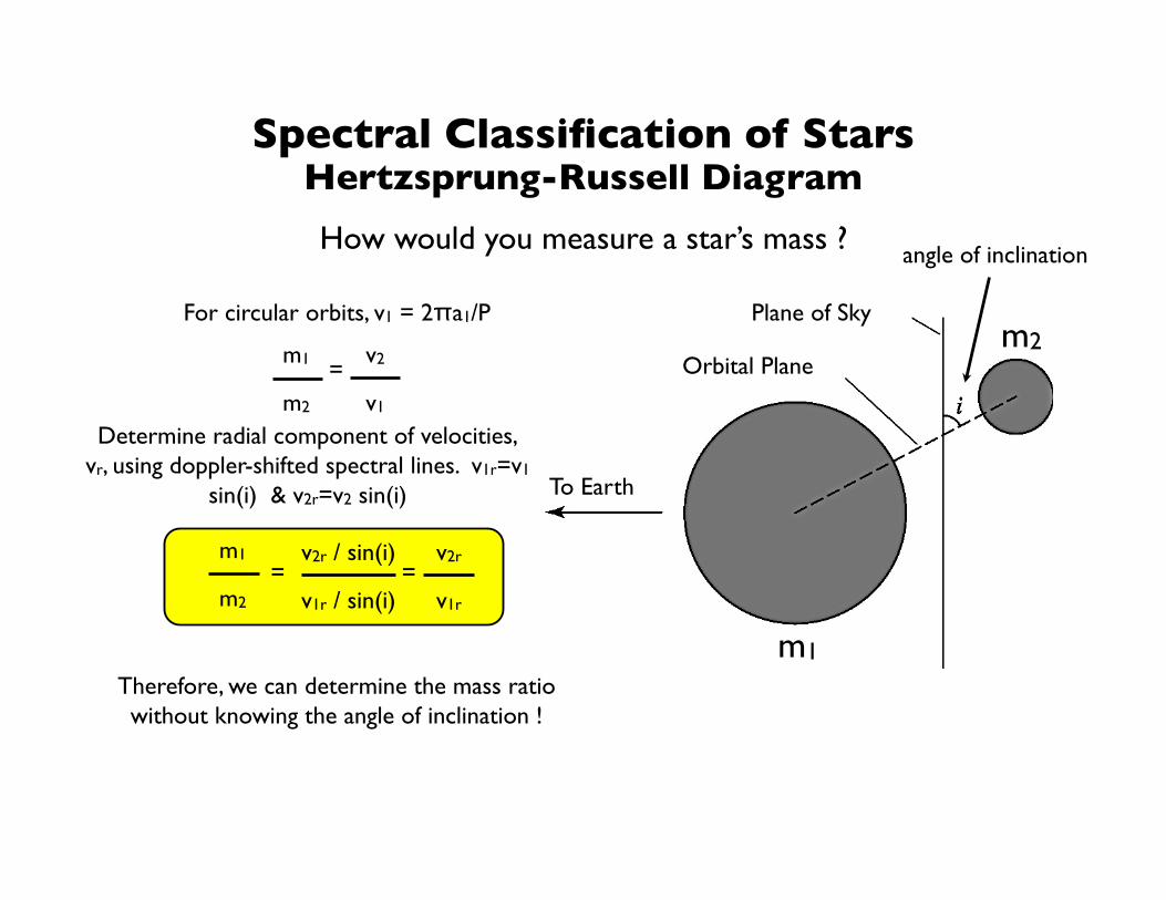
How would you measure a star’s mass ?
To Earth
Orbital Plane
Plane of Sky
m1
m2
v2
v1
=
For circular orbits, v1 = 2πa1/P
Determine radial component of velocities, vr, using doppler-shifted spectral lines. v1r=v1
sin(i) & v2r=v2 sin(i)
m1
m2
m1
m2
v2r / sin(i)
v1r / sin(i) =
v2r
v1r
=
Therefore, we can determine the mass ratio without knowing the angle of inclination !
angle of inclination
Hertzsprung-Russell Diagram
Spectral Classification of Stars
How would you measure a star’s mass ?
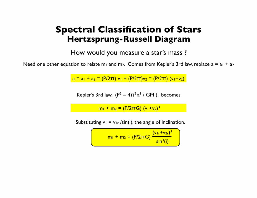
Need one other equation to relate m1 and m2. Comes from Kepler’s 3rd law, replace a = a1 + a2
a = a1 + a2 = (P/2π) v1 + (P/2π)v2 = (P/2π) (v1+v2)
Kepler’s 3rd law, (P2 = 4π2 a3 / GM ), becomes
m1 + m2 = (P/2πG) (v1+v2)3
Substituting v1 = v1r /sin(i), the angle of inclination.
m1 + m2 = (P/2πG) (v1r+v2r)3
sin3(i)
Hertzsprung-Russell Diagram
Spectral Classification of Stars
How would you measure a star’s mass ?
m1 + m2 = (P/2πG) (v1r+v2r)3
sin3(i)
m1
m2
v2r / sin(i)
v1r / sin(i) =
v2r
v1r
=
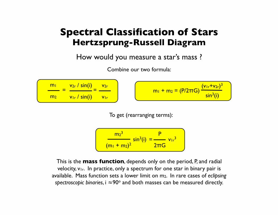
Combine our two formula:
To get (rearranging terms):
m23
(m1 + m2)2 sin3(i)
P v1r3 =
2πG
This is the mass function, depends only on the period, P, and radial velocity, v1r. In practice, only a spectrum for one star in binary pair is
available. Mass function sets a lower limit on m2. In rare cases of eclipsing spectroscopic binaries, i ≈90o and both masses can be measured directly.
Hertzsprung-Russell Diagram
Eclipsing Binaries:
http://instruct1.cit.cornell.edu/courses/astro101/java/eclipse/eclipse.htm
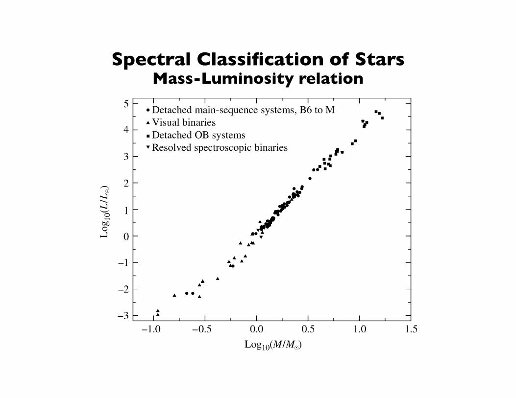
Spectral Classification of Stars Mass-Luminosity relation
Spectral Classification of Stars
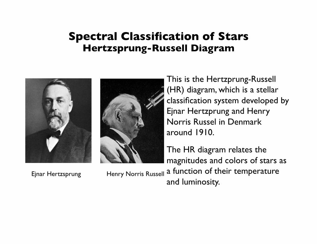
Ejnar Hertzsprung Henry Norris Russell
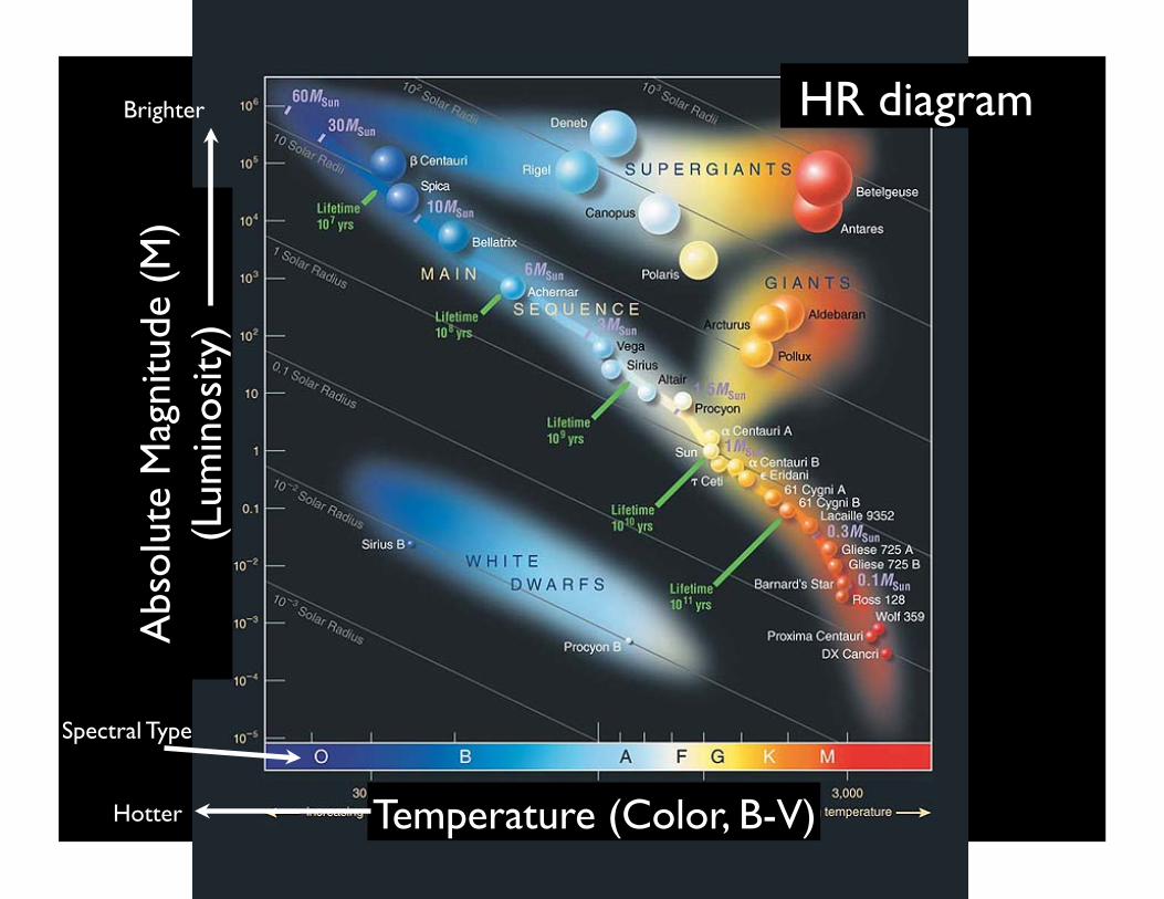
This is the Hertzprung-Russell (HR) diagram, which is a stellar classification system developed by Ejnar Hertzprung and Henry Norris Russel in Denmark around 1910.
The HR diagram relates the magnitudes and colors of stars as a function of their temperature and luminosity.
Hertzsprung-Russell Diagram
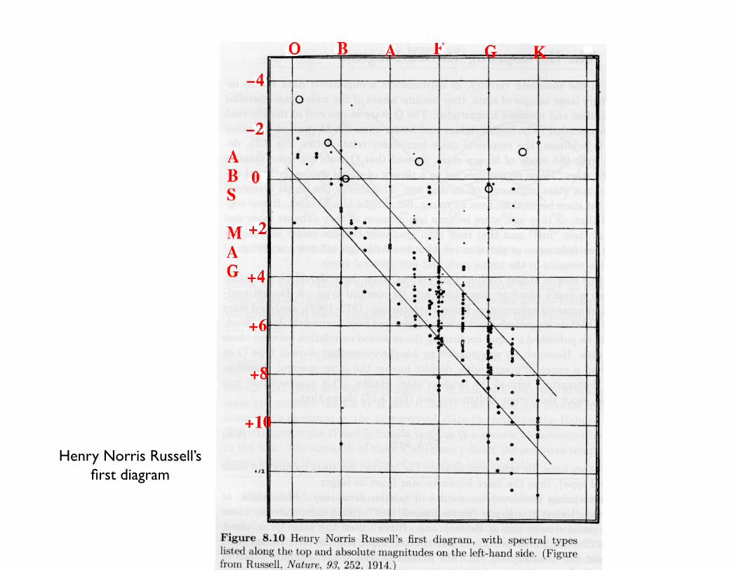
Henry Norris Russell’s first diagram
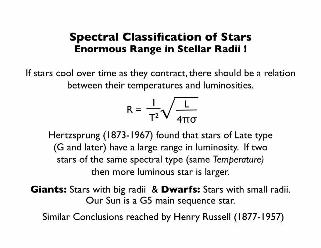
Spectral Classification of Stars Enormous Range in Stellar Radii !
If stars cool over time as they contract, there should be a relation between their temperatures and luminosities.
R = L 1
T2 4πσ √ Hertzsprung (1873-1967) found that stars of Late type (G and later) have a large range in luminosity. If two stars of the same spectral type (same Temperature)
then more luminous star is larger.
Giants: Stars with big radii & Dwarfs: Stars with small radii. Our Sun is a G5 main sequence star.
Similar Conclusions reached by Henry Russell (1877-1957)
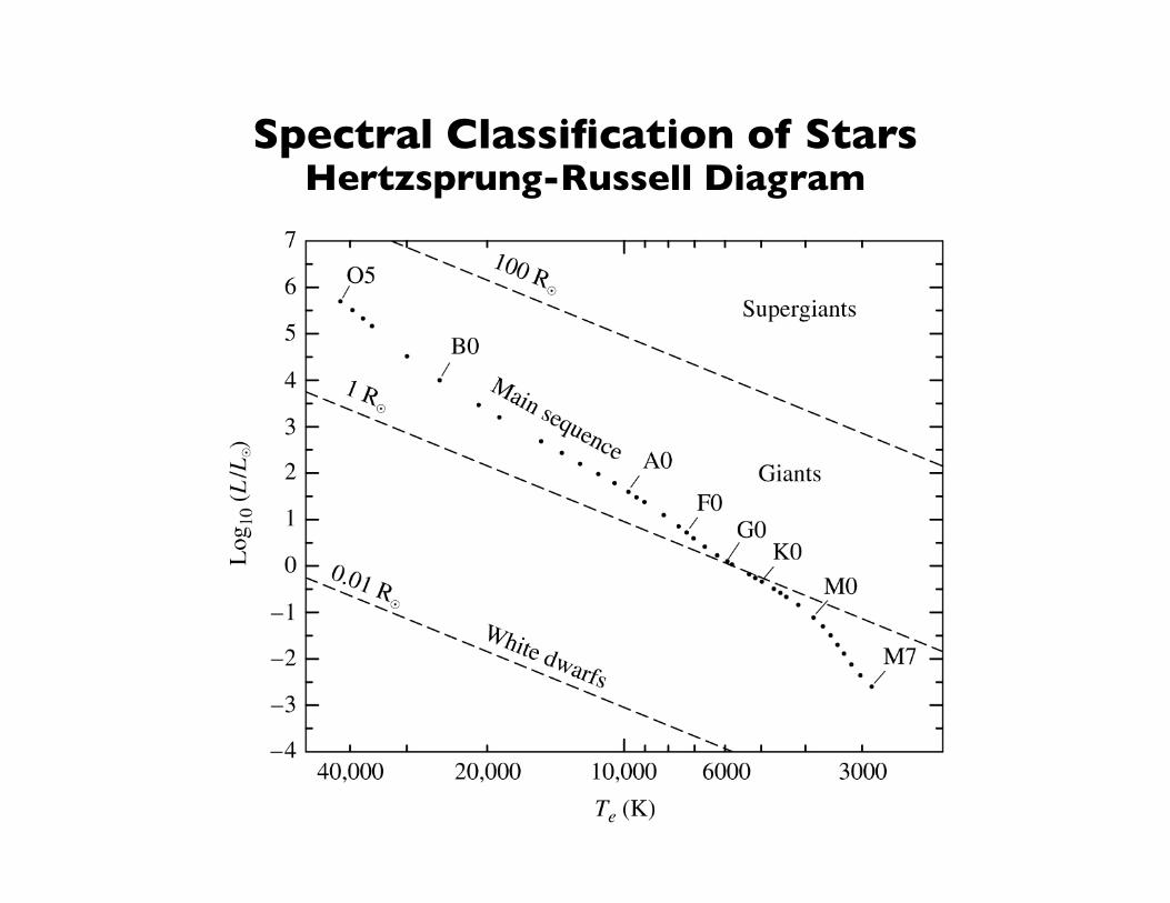
Spectral Classification of Stars Hertzsprung-Russell Diagram
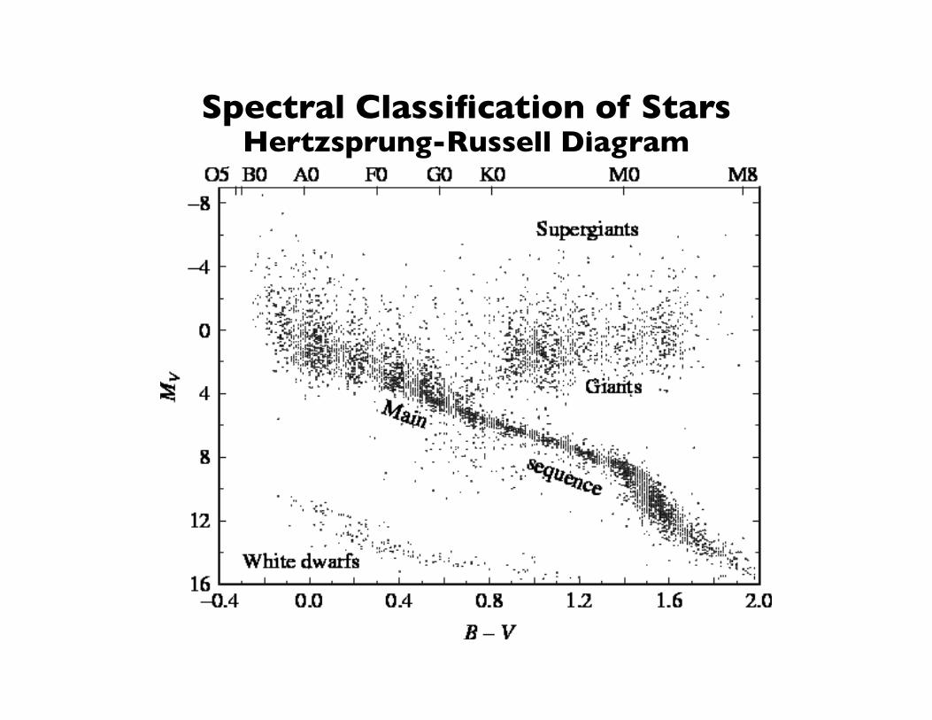
Spectral Classification of Stars Hertzsprung-Russell Diagram
Lum
inos
ity
Temperature: Hotter
Brighter
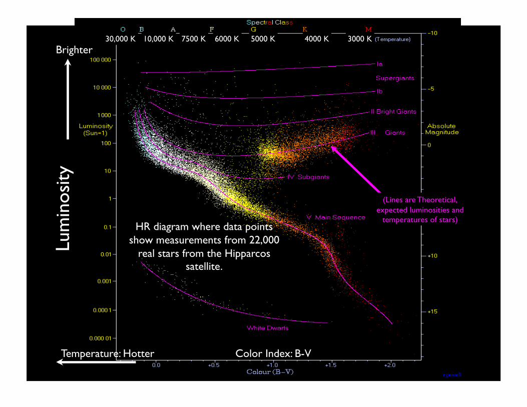
Text HR diagram where data points show measurements from 22,000
real stars from the Hipparcos satellite.
30,000 K 10,000 K 7500 K 6000 K 5000 K 4000 K 3000 K
(Lines are Theoretical, expected luminosities and
temperatures of stars)
Color Index: B-V
Abs
olut
e M
agni
tude
(M
) (L
umin
osity
)
Temperature (Color, B-V) Hotter
Brighter HR diagram
Spectral Type