sis sequential importance sampling advanced methods in simulation 096320 winter 2009 presented by:...
TRANSCRIPT
SISSequential Importance
Sampling
Advanced Methods In Simulation 096320
Winter 2009
Presented by: Chen Bukay, Ella Pemov, Amit Dvash

Talk Layout
SIS – Overview and algorithm Random walk – SIS simulation Nonlinear Filtering – Overview & Added
value Nonlinear Filtering – Simulation
Importance Sampling - General Overview
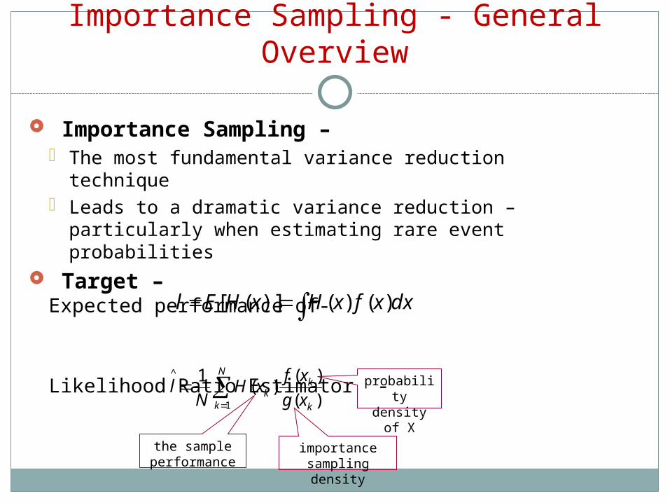
Importance Sampling – The most fundamental variance reduction
technique Leads to a dramatic variance reduction –
particularly when estimating rare event probabilities
Target – Expected performance of-
Likelihood Ratio Estimator -)(
)()(
1
1
^
k
kN
kk xg
xfxH
Nl
the sample performance
importance sampling density
probability density of X
dxxfxHxHEl )()()]([

SIS - Overview
Sequential Importance Sampling Also known as “Dynamic Importance Sampling”. Simply means importance sampling that carried out
in sequential manner.Why Sequential?
Problematic to sample from multi-dimensional vector Dependency between the variables It is difficult to sample from
),...,( 1 nxxx
f

SIS - Overview
Assumptions –
X is decomposable can present g(x) –
Easy to sample from g(x) sequentially
),...,|()...|()()( 1112211 nnn xxxgxxgxgxg

SIS – Overview (cont’)
It is easy to generate sequentially from Generate from Generate from …..We get –
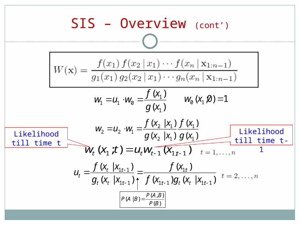
Due to the product rule of probability we can write -
The Likelihood function -
),...,|()...|()(
),...,|()...|()()(
1112211
11121
nnn
nn
xxxgxxgxg
xxxfxxfxfxW
1x
2x )|( 122 xxg
)(xg)( 11 xg
),...,|()...|()()( 11121 nn xxxfxxfxfxf)(
),()|(
BP
BAPBAP
),...,( 1 nxxx
SIS – Overview (cont’)
)(
)(
)|(
)|(
1
1
12
12122 xg
xf
xxg
xxfwuw
)();( 1;111 tttt xwutxw
Likelihood till time t
1)0;( 10 xw)(
)(
1
1011 xg
xfwuw
Likelihood till time t-1
)(
),()|(
BP
BAPBAP
)|()(
)(
)|(
)|(
1:11:1
:1
1:1
1:1
tttt
t
ttt
ttt xxgxf
xf
xxg
xxfu
SIS – Overview
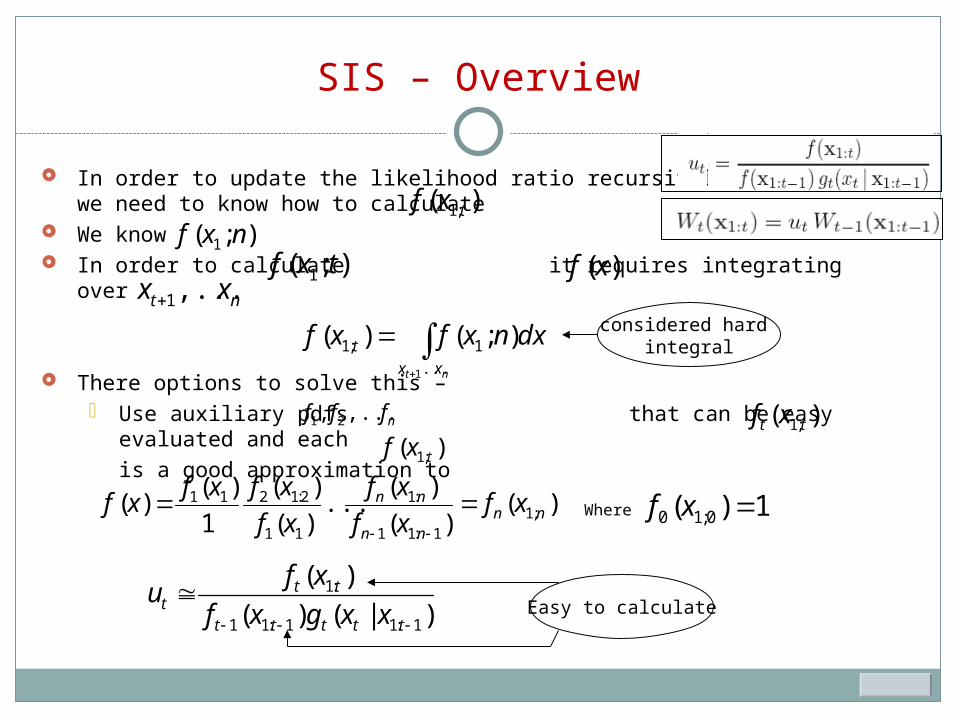
In order to update the likelihood ratio recursively, we need to know how to calculate
We know In order to calculate it requires integrating
over
There options to solve this – Use auxiliary pdfs that can be easy evaluated and each
is a good approximation to
);( 1 nxf);( 1 txf
)( ;1 txf
)(xfnt xx ,...,1
nfff ,...,, 21 )( ;1 tt xf)( ;1 txf
nt xx
t dxnxfxf...
1;1
1
);()( considered hard integral
Easy to calculate
Where 1)( 0;10 xf)()(
)(...
)(
)(
1
)()( ;1
1:11
:1
11
2:1211nn
nn
nn xfxf
xf
xf
xfxfxf
)|()(
)(
1:11:11
:1
ttttt
ttt xxgxf
xfu
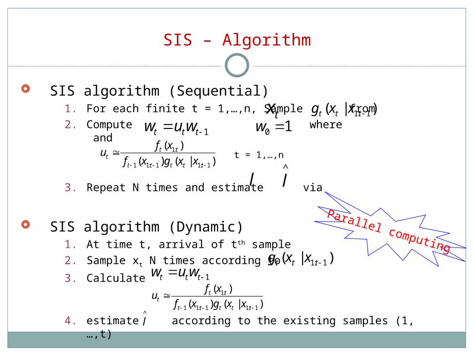
SIS – Algorithm
SIS algorithm (Sequential)1. For each finite t = 1,…,n, Sample from2. Compute where and
3. Repeat N times and estimate via
SIS algorithm (Dynamic) 1. At time t, arrival of tth sample2. Sample xt N times according to
3. Calculate
4. estimate according to the existing samples (1,…,t)
tx )|( 1:1 ttt xxg
1 ttt wuw 10 w
l^
l
1 ttt wuw
^
l
t = 1,…,n)|()(
)(
1:11:11
:1
ttttt
ttt xxgxf
xfu
)|( 1:1 ttt xxg
Parallel computing
)|()(
)(
1:11:11
:1
ttttt
ttt xxgxf
xfu

SIS Algorithm - Sequential
1st sample:
2nd sample:. .. .. .Nth sample:
2 1( ,..., )nx xx
1 1( ,..., )nx xx
1( ,..., )N nx xx
Calculate )(1 xw
Calculate
Calculate )(xwN
)(2 xw
Estimate by Computing )()(1
1
^
k
N
kk xWxH
Nl
l

SIS Algorithm - Dynamic
1st sample:
2nd sample:.
..
..
.Nth sample:
),...,( 1 nxx1x
At Timet =1
)( 1x2x
)( 1x1x
),...,( 1 nxxNx
)(1 xw
)(xwN
)(2 xw
)()(1
1
^
kk xx WHN
lN
k
l
),( 21 xx1x
)( 1xNx ),( 21 xxNx
),...,( 1 nxx2x ),( 21 xx2x
Calculaterecalculate
recalculateCalculate
Calculaterecalculate
At time t =2
At time t=n
Estimate by Computing
With the existing samples)](),..([ 1 xwxwW t
Nt
t
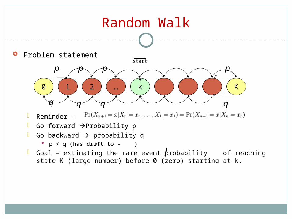
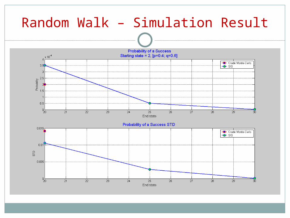
Random Walk
Problem statement
Reminder - Go forward Probability p Go backward probability q
p < q (has drift to - ) Goal – estimating the rare event probability of reaching state K (large
number) before 0 (zero) starting at k.l
p
0 K1 2 … k
q
p
qqq
p p pstart
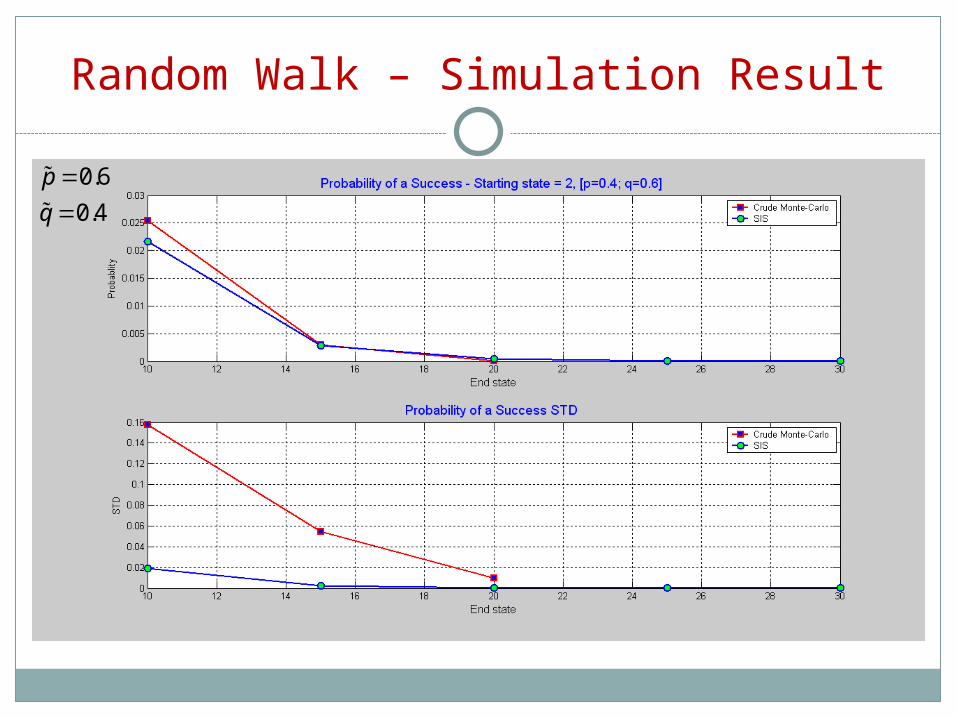
Random Walk – Simulation Result
0.6
0.4
p
q
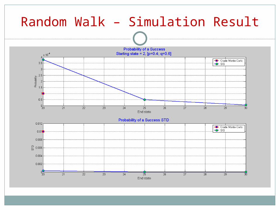
Random Walk – Simulation Result

Random Walk – Simulation Result
0.8
0.2
p
q
Random Walk – Simulation Result

SIS Application:
Non Linear Filtering

State Space Models
( )1 kk kx x V T w
( ) k kky x v
x
Tx1 x2 x3
y2 y3y1
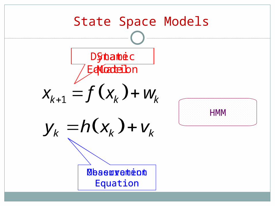
State Space Models
k k ky h x v
Dynamic Model
Measurement Equation
State Equation
Observation Equation
1k k kx f x w HMM

State Space Models cont’
k k ky h x v
1k k kx f x w Known pdf - Pw
Known pdf - Pv
Markov Property1 |
|k k w
k k v
x x P
y x P

Linear Models
Kalman Filter Linear Dynamic models Linear Measurement Equations v, w, x0 – Gaussian & independent
Kalman Filter is the optimal estimator (MSE)
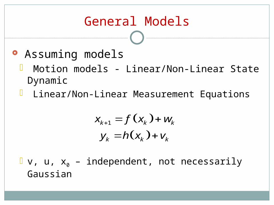
Assuming models Motion models - Linear/Non-Linear State
Dynamic Linear/Non-Linear Measurement Equations
v, u, x0 – independent, not necessarily Gaussian
General Models
1
k k k
k k k
x f x w
y h x v

Problem Description
θa
θb
θc
LOP – Line Of Position
Observers – Known exact location
(xa,,ya)
(xb,yb)
(xc,,yc)
Target – Unknown location
(xe,,ye)

θa
θb
θc
Bearing Only Measurements
(xe,,ye)
(xa,,ya)
(xb,yb)
(xc,,yc)
tan e
e
c
c
y yc
xx

Bearing Only Measurements
2
tan1
kk k
k
xy v
x
1k k kx x w
1 | ,
2| tan ,
1
k k k
kk k
k
x x N x Q
xy x N R
x

Non-Linear Filtering
Motivation Non linear dynamic/measurement equations Noise distribution not Gauss
Kalman Filter: No longer the optimal estimator (MSE)
EKF – Linearization of the state space Equations Suboptimal estimator Convergence is not guaranteed

The Bootstrap Filter
Represent the pdf as a set of rv (and not as a function)
The Bootstrap Filter – Recursive algorithm for propagating and updating these rv samples
Samples are naturally concentrated in regions of high probability
“Novel Approach to nonlinear/non Gaussian Bayesian state estimation” N.J. Gordon, D.J. Salmond & A.F.M Smith

Motivation For having P(X(k)|Y(1:k))
1:1
ˆ |N
i iN k k k k k
i
p x Y q x x
ˆ: |MSE x E x y
MSE
ˆ: arg max |x
ML x f y x
ML

The Bootstrap FilterRecursive Calculation of P(X(k)|Y(1:k))
1: 1
1: 11:
11
:
| || |
|| t t t t
tt t t tt t
t
P y x P x yP y x P x y
P yx y
yP
1: 1 1 1 1: 1 1| | |t t t t t t tP x y P x x P x y dx
1 1|t t w t tP x x P x f x
|t t v t tP y x P y h x 1 1: 1|t tP x y
Assume we know
Bayes & yt|xt independent of y1:t-1

The importance Sampling
1: 1: 1| | |
t t tg xf x w
t t t t t tP x y P y x P x y
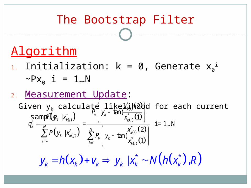
The Bootstrap Filter
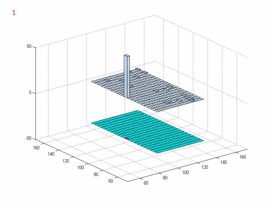
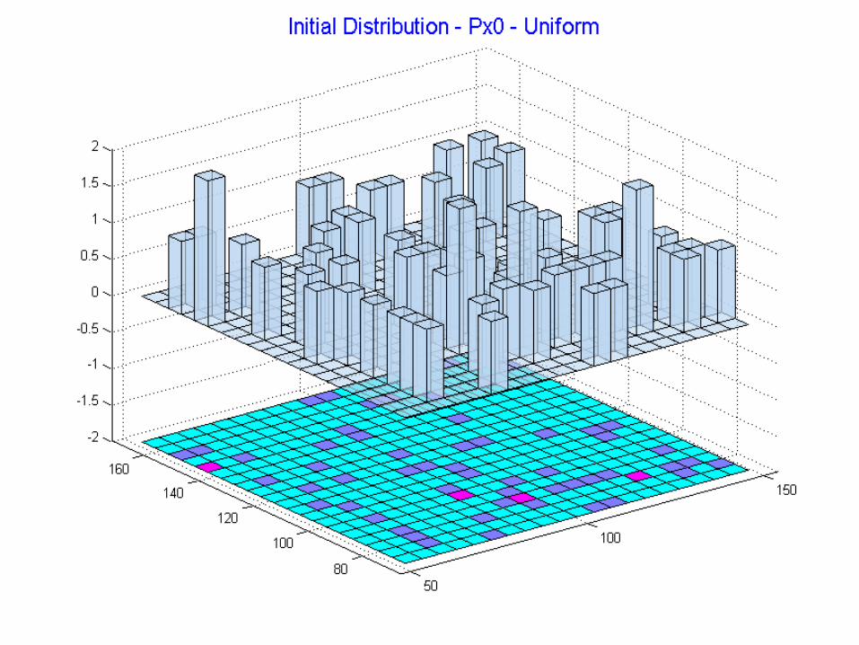
Algorithm1. Initialization: k = 0, Generate x0
i ~Px0 i = 1…N
2. Measurement Update:Given yk calculate likelihood for each current sample
*
* *
**
*11
2tan(
| 1 = i = 1...N
2| tan(1
k i
v kk k i k ii
k NN
k ik k j
v kjj k i
xP y
P y x xq
xP y x P yx
* *| ,k k k k k ky h x v y x N h x R

Algorithm (cont’)
3. Re-Sampling - Sample N samples from {xk
*i}i=1:N, with replacement, where the probability to choose the i-th particle is qk
i at stage k
4. Prediction: Pass the new samples through the system Equation
5. Set k = k+1 and return to 2
The Bootstrap Filter
*
1 ,k k kk i k ix f x w x w

-50 0 50 100 150 200 2500
50
100
150Problem Geometry
X-Axis [km]
Y-Ax
is [k
m]
Target True Poistion (141,141)Initial Estimation Of Target Poistion (100,120)Observer Course
Vx= -0.1 [km/sec]
Vy= 0.01 [km/sec]
dt = 300 [sec]
Measurement Variance ~ 1o
(141,,141) [km]
(100,120) [km]

1

2

3

4

5

6
7

8

1

2

3

4
5

6

7


1 2 3 4 5 6 7 8 9 10 110
500
1000
1500
2000
Measurement index
MS
E
The Effect of Resampling on the MSE[1000 particles; 1e3 - Monte-Carlo Simulations]
BSF with Resampling - X-Axis position estimation
BSF No Resampling - X-Axis position estimation
1 2 3 4 5 6 7 8 9 10 110
200
400
600
800
Measurement index
MS
E
BSF with Resampling - Y-Axis position estimation
BSF No Resampling - Y-Axis position estimation

-150 -100 -50 0 50 100 1500
50
100
150Problem Geometry
X-Axis [km]
Y-A
xis
[km
]
Target True Poistion (141,141)
Initial Estimation Of Target Poistion (100,120)
Observer CourseBSF With Resampling
BSF No Resampling

95 100 105 110 115 120 125 130 135 140 145
115
120
125
130
135
140
145
Problem Geometry
X-Axis [km]
Y-A
xis
[km
]
Target True Poistion (141,141)
Initial Estimation Of Target Poistion (100,120)
Observer CourseBSF With Resampling
BSF No Resampling

Simulations
1
3tan
1
k k k
kk k k
k
x Fx Gw
xy x v
x
1 0 0
0 1 0 0
0 0 1
0 0 0 1
T
GT
1 0 0
0 1 0 0
0 0 1
0 0 0 1
T
FT
1
_
_
_
_
k
x position
x velocityx
y position
y velocity

0 50 100 150 200 250 300 350 400 450
-150
-100
-50
0
X-Axis [km]
Y-A
xis
[km
]Initial Conditions: x & y -petrubations among its error variance
Observer Location (0,0)
Target True Location
Initial Estimation Of Target PoistionEKF
BSF
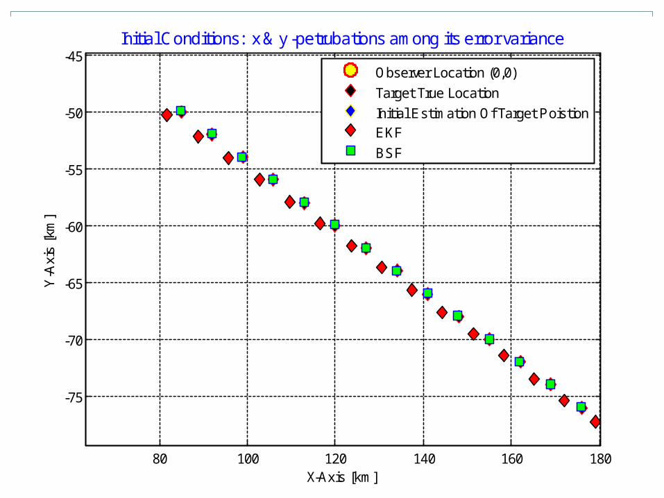
80 100 120 140 160 180
-75
-70
-65
-60
-55
-50
-45
X-Axis [km]
Y-A
xis
[km
]Initial Conditions: x & y -petrubations among its error variance
Observer Location (0,0)
Target True Location
Initial Estimation Of Target PoistionEKF
BSF

0 50 100 150 200 250 300 350 400 450
-140
-120
-100
-80
-60
-40
-20
0
X-Axis [km]
Y-A
xis
[km
]
Initial Conditions: x-petrubation ~0 y-petrubation 5.5
Observer Location (0,0)
Target True Location
Initial Estimation Of Target PoistionEKF
BSF
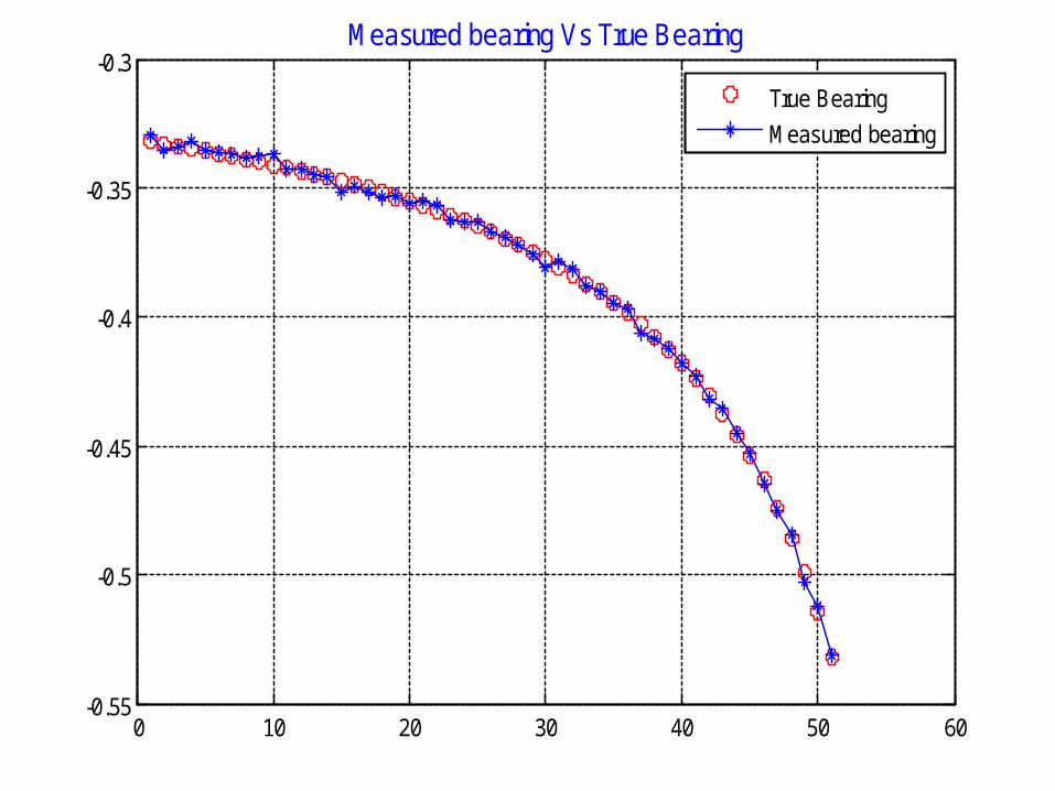
0 10 20 30 40 50 60-0.55
-0.5
-0.45
-0.4
-0.35
-0.3Measured bearing Vs True Bearing
True Bearing
Measured bearing

0 50 100 150 200 250 300 350
-150
-100
-50
0
50
100
150
200
X-Axis [km]
Y-A
xis
[km
]
Initial Conditions: x & y -petrubations among its error variance
Observer Location (0,0)
Target True Location
Initial Estimation Of Target PoistionEKF
BSF
150 time steps

0 20 40 60 80 100 120 140 160-1.4
-1.2
-1
-0.8
-0.6
-0.4
-0.2
0
0.2
0.4
0.6Measured bearing Vs True Bearing
True Bearing
Measured bearing

20 30 40 50 60 70 80 90136
138
140
142
144
146
148
150
152
154
156
X-Axis [km]
Y-A
xis
[km
]Initial Conditions: large x-y petrubations
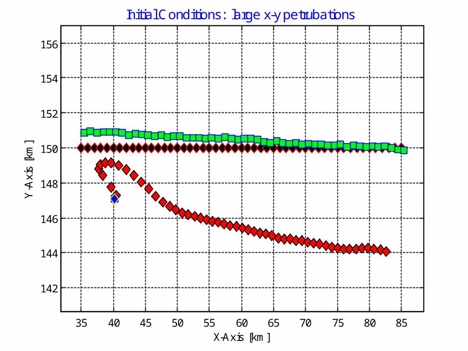
35 40 45 50 55 60 65 70 75 80 85
142
144
146
148
150
152
154
156
X-Axis [km]
Y-A
xis
[km
]Initial Conditions: large x-y petrubations

0 20 40 60 80 100 120 140
50
100
150
200
250
300
X-Axis [km]
Y-A
xis
[km
]
Initial Conditions: large x-y petrubations


Backup

Markov Chain
Markov property – Given the present state, future states are independent of the past states. The present state fully captures all the information that could influence the
future evolution of the process.
The changes of state are called transitions, and the probabilities associated with various state-changes are called transition probabilities.
210.9
0.1
0.5
0.50.9 0.10.5 0.5
P=

F(X) - calculations
)(
),()|(
BP
BAPBAP
),...,,(),...,(
),...,,(...
)(
),(
1
)()( 21
11
21
1
211n
n
n xxxfxxf
xxxf
xf
xxfxfxf
),...,|()...|()()( 11121 nn xxxfxxfxfxf
)()(
)(...
)(
)(
1
)()( ;1
1:11
:1
11
2:1211nn
nn
nn xfxf
xf
xf
xfxfxf
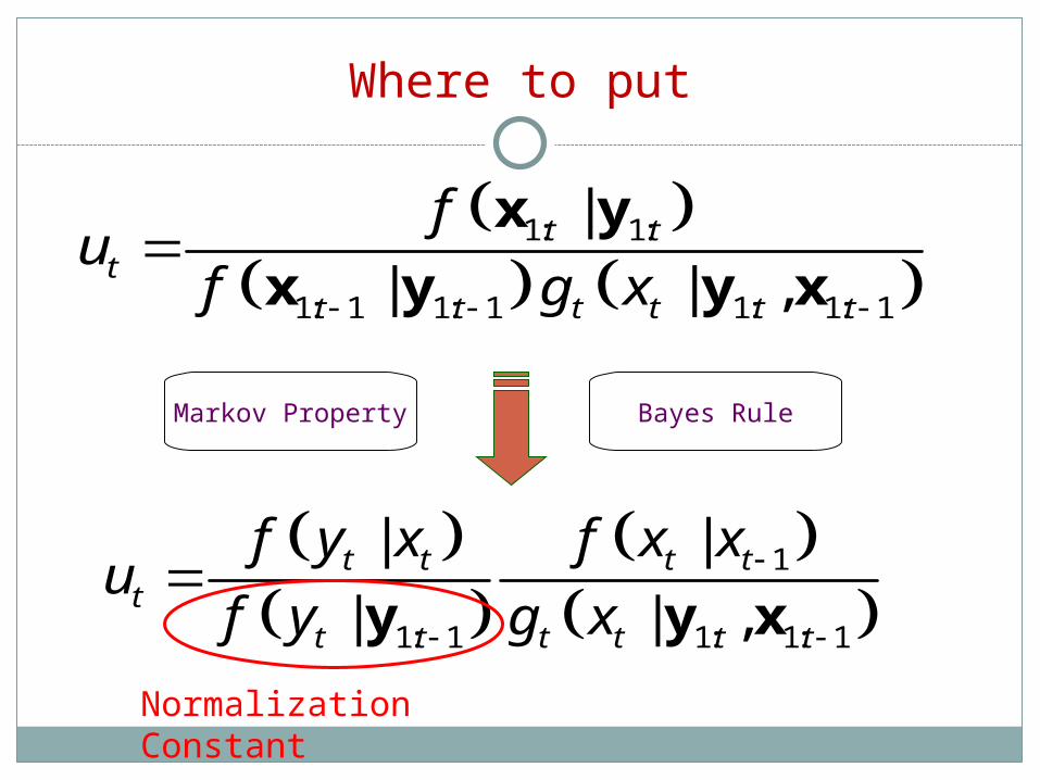
Where to put
1: 1:
1: 1 1: 1 1: 1: 1
|
| | ,t t
tt t t t t t
fu
f g x
x y
x y y x
1
1: 1 1: 1: 1
| |
| | ,t t t t
tt t t t t t
f y x f x xu
f y g x
y y x
Markov Property Bayes Rule
Normalization Constant

Where to put 2
1
1: 1: 1
| |
| ,t t t t
tt t t t
f y x f x xu
C g x
y x
|t tt
f y xu
C
1: 1: 1 1| , |t t t t t tg x f x x y x