21-7 12/10 JTRP-2010/26 INDOT Office of Research & Development West Lafayette, IN 47906

INDOT Research

TECHNICAL Summary Technology Transfer and Project Implementation Information

TRB Subject Code: 21-7 Safety Appurtenances Design and Placement December 2010

Publication No. FHWA/IN/JTRP-2010/26, SPR-3064 Final Report

SITE VERIFICATION OF WEIGH-IN-MOTION TRAFFIC AND

TIRTL CLASSIFICATION DATA

Introduction

Quality weigh-in-motion (WIM) traffic data is

essential not only in general transportation application,

but also in pavement design. The new AASHTO

Mechanistic-Empirical Pavement Design Guide for New

and Rehabilitated Pavement Structures (MEPDG)

requires information on the detailed truck traffic, such as

truck traffic volume, truck traffic monthly and hourly

variations, vehicle class distribution, axle load, and axle

load distributions, instead of the traditional ESALs. In

addition, the Indiana Department of Transportation

(INDOT) needs to collect traffic data frequently so as to

timely provide accurate traffic information for planning,

program development, operations, and pavement

management. Currently, INDOT is using the pneumatic

road traffic counters in traffic data collection, such as

particular short-term or temporary traffic data collections.

However, the pneumatic road traffic counter requires

installation of rubber tubes on the pavement surface. As a

result, the installation of rubber tubes usually creates

safety issues to our workers and is timely consuming and

labor intensive. Therefore, it is an urgent need for

INDOT to utilize new devices to enhance the safety of

field traffic data collection without compromising data

quality.

This study consists of two parts. The first part is to

verify the accuracy of WIM vehicle classification and

develop models for vehicle classification corrections

using image processing technologies. The second part is

to install and then evaluate a traffic surveillance system,

i.e., the Transportable Infra-Red Traffic Logger

(TIRTL). In the first part, the investigators collected

video and WIM traffic data at WIM sites statewide. A

digital image based vehicle monitoring and

classification system was developed for verifying

weigh-in-station data, in particular the vehicle

classification counts. Based on the real world WIM and

video traffic classification data, allocation factors were

determined for correcting the unclassified vehicle

counts associated with the WIM traffic data.

In the second part of this study, a TIRTL system

was installed to collect traffic data near a WIM site.

Hourly traffic data was first gathered manually and by

video cameras to verify the potential errors associated

with the TIRTL vehicle counts. Large amount of daily

WIM traffic data was also utilized as baseline data to

evaluate the field performance of TIRTL and assess the

impact of various weather conditions, such as fog, rain

and snow, and thunderstorm on TIRTL’s performance.

The evaluation was based on the FHWA Scheme F

Vehicle Classification and solely a data-driven process..

Findings

The digital image based vehicle monitoring and

classification system developed by this study is user

friendly and can be easily to setup, and perform data

acquisition, vehicle monitoring, and length-based

vehicle classification. This system can help develop the

models for correcting weigh-in-station data, in

particular the unclassified vehicle counts. It was shown

that the traditional method to treat all unclassified

vehicle counts as trucks is too conservative and will

largely overestimate the truck traffic volume. Video

technologies can provide accurate and effective vehicle

detection when vehicles are classified into four

categories, including two-axle, four-tire vehicles, single

unit trucks, single-trailer trucks, and multi-trailer

trucks.

WIM sensor malfunction can generate serious

vehicle classification issues. The percentage of

unclassified vehicles increases as vehicle counts

increases. As the number of travel lanes increases, the

possibility for vehicles to execute lane changing or

passing increases. Therefore, more vehicles may

occupy two adjacent lanes or change speeds on sensors,

leading to greater percentages of unclassified vehicles.

It becomes unacceptable when the percentage of

unclassified vehicles exceeds 4% for a single lane.

Based on the WIM data statewide, the unclassified

vehicles mainly involved single tractor trailers and

passenger cars. Single unit trucks were most likely

classified by WIM. While traffic volume and lane

number are the two main contributing factors, it is

21-7 12/10 JTRP-2010/26 INDOT Office of Research & Development West Lafayette, IN 47906

unrealistic to predict the unclassified vehicles in terms

of traffic volume and lane number at this time. Overall,

vehicles under Categories 1, 2, 3, and 4 account

respectively for 35%, 5%, 48%, and 12% of the total

unclassified vehicles.

Under clear weather conditions, the TIRTL vehicle

counts agreed very well with the manual and video

vehicle counts, respectively. When vehicles are

classified into four categories, such as two-axle, four-

tire vehicles, single unit trucks, single-trailer trucks, and

multi-trailer trucks, the accuracy of vehicle

classification for Category 1, including all two-axle,

four-tire vehicles, was better than that for tractor

trailers. WIM vehicle counts were utilized to validate

the performance of TIRTL system. Unlike WIM

system, the number of unclassified vehicles by TIRTL

was very small.

For axle-based vehicle classification, i.e., the 13-

class FHWA vehicle classification scheme, great

discrepancies existed between the WIM and TIRTL

vehicle class counts. Both WIM and TIRTL

demonstrated difficulties to distinguish Class 3 from

Class 2. However, TIRTL demonstrated better

performance to identify vehicles under Class 3 than

WIM, regardless of weather conditions. Under Class 5,

the TIRTL vehicle counts were more reasonable than

the WIM vehicle counts. The WIM system might over-

count vehicles under Class 5. Based on the default truck

class distributions, TIRTL might provide vehicle

classification more accurate than WIM. Under normal

weathers, fog, snow, and rain did not affect TIRTL’s

performance. Under thunderstorm weather, however,

TIRTL might undercount vehicles regardless of vehicle

class.

Implementation

The findings on WIM vehicle classification will be

utilized by the INDOT Office of Research and

Development to adjust truck traffic volumes and vehicle

class distribution for the implementation of the new

AASHTO MEPDG statewide. The adjustment factors

can be used to make corrections on the truck traffic

volume and allocate the unclassified vehicles based on

vehicle categories.

The findings on TIRTL traffic data collection are

intended to assist INDOT Traffic Monitoring Section in

assessing the accuracy of TIRTL vehicle classification

data and its field performance under various weather

conditions. Necessary training will be provided to

INDOT pavement designers.

Contacts

For more information:

Shuo Li

Indiana Department of Transportation

Office of Research and Development

West Lafayette, IN 47906

Phone: 765-463-1521

Fax: 765-497-1665

Email: [email protected]

Purdue University

Joint Transportation Research Program

School of Civil Engineering

West Lafayette, IN 47907-1284

Phone: (765) 494-9310

Fax: (765) 496-7996

E-mail: [email protected]

http://www.purdue.edu/jtrp

mailto:[email protected]

mailto:[email protected]

http://www.purdue.edu/jtrp



Site Verification of Weigh-In-Motion Traffic and TIRTL Classification Data

By

Shuo Li, Ph.D., P.E.

Research and Pavement Friction Engineer

Office of Research and Development


Yingzi (Eliza) Du, Ph.D., Assistant Professor

Department of Electrical and Computer Engineering

IUPUI

Indianapolis, IN 46202

And

Yi Jiang, Ph.D., P.E., Associate Professor

Department of Building Construction Management

Purdue University

West Lafayette, IN 47907


Project No. C-36-59XXX

File No. 08-05-50

SPR-3064

Prepared in Cooperation with the

Indiana Department of Transportation and the

U.S. Department of Transportation

Federal Highway Administration

The contents of this report reflect the views of the author who is responsible for the facts and the

accuracy of the data presented herein. The contents do not necessarily reflect the official views

or policies of the Indiana Department of Transportation or the Federal Highway Administration

at the time of publication. This report does not constitute a standard, specification, or regulation.

Purdue University

West Lafayette, Indiana 47907

December, 2010

TECHNICAL REPORT STANDARD TITLE PAGE 1. Report No. 2. Government Accession No. 3. Recipient's Catalog No.


4. Title and Subtitle Site Verification of Weigh-In-Motion Traffic and TIRTL Classification Data

5. Report Date

December 2010

6. Performing Organization Code

7. Author(s)

Shuo Li, Yingzi (Eliza) Du, Yi Jiang

8. Performing Organization Report No.


9. Performing Organization Name and Address


1284 Civil Engineering Building

Purdue University

West Lafayette, Indiana 47907-1284

10. Work Unit No.

11. Contract or Grant No.

SPR-3064

12. Sponsoring Agency Name and Address


State Office Building

100 North Senate Avenue

Indianapolis, IN 46204

13. Type of Report and Period Covered

Final Report

14. Sponsoring Agency Code

15. Supplementary Notes

Prepared in cooperation with the Indiana Department of Transportation and Federal Highway Administration.

16. Abstract

Quality weigh-in-motion (WIM) traffic data is essential not only in general transportation application, but also in pavement design.

The new AASHTO Mechanistic-Empirical Pavement Design Guide (MEPDG) for New and Rehabilitated Pavement Structures requires

information on the detailed truck traffic, such as truck traffic volume, truck traffic monthly and hourly variations, vehicle class

distribution, axle load, and axle load distributions, instead of the traditional ESALs. In addition, the Indiana Department of Transportation

(INDOT) needs to collect traffic data frequently so as to timely provide accurate traffic information for planning, program development,

operations, and pavement management. Currently, INDOT is using the pneumatic road traffic counters in traffic data collection, such as

particular short-term or temporary traffic data collections. However, the pneumatic road traffic counter requires installation of rubber tubes

on the pavement surface. As a result, the installation of rubber tubes usually creates safety issues to our workers and is timely consuming

and labor intensive. Therefore, it is an urgent need for INDOT to utilize new devices to enhance the safety of field traffic data collection

without compromising data quality.

This study consists of two parts. The first part is to verify the accuracy of WIM vehicle classification and develop models for

vehicle classification corrections using image processing technologies. The second part is to install and then evaluate a traffic surveillance

system, i.e., the Transportable Infra-Red Traffic Logger (TIRTL). In the first part, the investigators collected video and WIM traffic data

at WIM sites statewide. A digital image based vehicle monitoring and classification system was developed for verifying weigh-in-station

data, in particular the vehicle classification counts. Based on the real world WIM and video traffic classification data, allocation factors

were determined for correcting the unclassified vehicle counts associated with the WIM traffic data.

In the second part of this study, a TIRTL system was installed to collect traffic data near a WIM site. Hourly traffic data was first

gathered manually and by video cameras to verify the potential errors associated with the TIRTL vehicle counts. Large amount of daily

WIM traffic data was also utilized as baseline data to evaluate the field performance of TIRTL and assess the impact of various weather

conditions, such as fog, rain and snow, and thunderstorm on TIRTL’s performance. The evaluation was based on the FHWA Scheme F

Vehicle Classification and solely a data-driven process.

17. Key Words

Weigh-in-motion, vehicle tracking, traffic monitoring, dynamic

content based image segmentation, vehicle classification, infra-

red light technology, weather condition

18. Distribution Statement

No restrictions. This document is available to the public through the

National Technical Information Service, Springfield, VA 22161

19. Security Classif. (of this report)

Unclassified

20. Security Classif. (of this page)

Unclassified

21. No. of Pages

60

22. Price

Form DOT F 1700.7 (8-69)

i

TABLE OF CONTENTS

TABLE OF CONTENTS…i

LIST OF TABLES …iii

LIST OF FIGURES…iv

ACKNOWLEDGMENTS…v

CHAPTER 1

INTRODUCTION………………………………………………………………........................1

Background…………………………………………………………………………………1

Problem Statement………………………………………………………………………….2

Objectives…………………………………………………………………………………..4

Main Tasks and Research Approach……………………………………………………….4

CHAPTER 2 DEVELOPMENT OF DYNAMIC CONTENT BASED VEHICLE

TRACKING AND TRAFFIC MONITORING SYSTEM…………………....8

Overview……………………………………………………………………………………8

Traditional Vehicle Categories…………………………………………………………….11

Approach for Digital Image Processing……………………………………………………11

The Video Image Processing System……………………………………………………...31

CHAPTER 3 VALIDATION OF WIM VEHICLE CLASSIFICATION DATA USING

VIDEO COUNTS ………………………………………………………………33

WIM Vehicle Classification Data………………………………………………………….33

Video Vehicle Classification Data…………………………………………………………35

Data Analysis………………………………………………………………………………37

CHAPTER 4 EVALUATION OF TIRTL’S FIELD PERFORMANCE …………………..43

The TIRTL Vehicle Data Collection………………………………………………………43

ii

Validation of TIRTL Data Accuracy by Manual Vehicle Counts…………………………44

Comparison of TIRTL and WIM Vehicle Counts…………………………………………47

CHAPTER 5 IMPACT OF WEATHER CONDITIONS ON TIRTL’S PERFORMANCE

…...52

The TIRTL System Operations…………………………………………………………….52

Impact of Weather Conditions……………………………………………………………..53

CHAPTER 6 CONCLUSIONS ……………………………………………………………….56

Video Vehicle Detection and Classification………………………………………………56

WIM Vehicle Detection and Classification……………………………………………….57

TIRTL Vehicle Detection and Classification……………………………………………..57

References………………………………………………………………………………………58

iii

LIST OF TABLES

Table 2-1 Four Traditional Vehicle Categories

Table 3-1 WIM Vehicle Classification Data at Selected WIM Sites

Table 3-2 Video Vehicle Classification Data at WIM Sites

Table 3-3 Summaries of Percentages of Unclassified Vehicles for Each WIM Lane

Table 3-4 Comparison of Vehicle Category Distributions

Table 3-5 Adjustment Factors of Unclassified Vehicles

Table 4-1 Comparison of Manual and TIRTL Vehicle Counts

Table 4-2 Comparison of Video and WIM Vehicle Counts

Table 4-3 Comparison of WIM and TIRTL Daily Vehicle Class Counts

Table 5-1 Percent Errors in Clear Weather

Table 5-2 Percent Errors in Foggy Weather

Table 5-3 Percent Errors in Normal Snowy Weather

Table 5-4 Percent Errors in Wet Weather

iv

LIST OF FIGURES

Figure 1-1 Unclassified Vehicle Counts

Figure 1-2 Effects of Unclassified Vehicles on Pavement Cracking

Figure 2-1 The Problems of the Traditional Segmentation Assumptions

Figure 2-1 FHWA 13 Vehicle Classes

Figure 2-3 Flow Chart for the Frame Subtraction Method

Figure 2-4 Examples of Vehicles over Multiple Lanes

Figure 2-5 Illustration of the Separation Process

Figure 2-6 Demonstration of Object Projection from 3D to 2D (20)

Figure 2-7 Linear Projective Geometry, Image from (21)

Figure 2-8 Fundamental Theorem of Similarity, Image from (21)

Figure 2-9 Parallel Lines in Projective Planes (Menelaus’s Theorem), Image from (21)

Figure 2-10 Cross Ratio, Image from (21)

Figure 2-11 Example of a Video Frame with Shadow

Figure 2-12 Shadow Removal Algorithm

Figure 2-13 Mean Shift Clustering Results

Figure 2-14 Adaptive Thresholding Result

Figure 2-15 Incorrect Cluster Connection

Figure 2-16 Correct Cluster Connection

Figure 2-17 Results from the Shadow Detection and Removal Algorithm

Figure 2-18 Full View of the Software

Figure 3-1 Camcorder Setting

Figure 3-2 Variations of Unclassified Vehicles with Traffic Volume

Figure 3-3 Variations of Unclassified Vehicles with Number of Lanes

Figure 3-4 Comparison of WIM and Video Vehicle Counts

Figure 4-1 TIRTL System Installed on I-65 in Lafayette, IN

Figure 4-2 Graphical Illustration of TIRTL and WIM Sites

Figure 4-3 Lane Configuration

Figure 4-4 Vehicle Class Distributions by WIM and TIRTL

Figure 4-5 Comparison of Truck Class Distributions

Figure 5-1 Configuration of TIRTL Infra-Red Light Beams

v

ACKNOWLEDGMENTS

This research project was sponsored by the Indiana Department of Transportation

(INDOT) in cooperation with the Federal Highway Administration through the Joint

Transportation Research Program (JTRP). The authors would like to thank the study advisory

committee members, Kirk Mangold, Tommy Nantung, and Samy Noureldin for their valuable

assistance and technical guidance in the course of performing this study. Sincere thanks are

extended to Larry Torrance of the INDOT and Robb Bingham of Control Specialists Company

for their assistance in data collection and system evaluation.

1

Chapter 1

INTRODUCTION

Background

In the past decades, vehicle classification data has been widely used in transportation

planning, highway operations, traffic analysis, and performance measurements. This data serves

as the starting point for other needed transportation statistics, including truck vehicle miles

traveled (VMT), and freight tonnage carried by trucks along certain roadways or on the whole

highway network. In addition, this data has been utilized to estimate the traffic load design inputs

such as equivalent single axle loads (ESALs) for pavement structural design and to calculate the

pavement remaining life for pavement management systems. Recently, a new pavement design

guide, the AASHTO Mechanistic-Empirical Pavement Design Guide (MEPDG) (1) was released

as a tool for the design and analysis of new and rehabilitated pavement structures.

The AASHTO MEPDG utilizes a comprehensive suite of design inputs to design

pavements with enhanced reliability and desired performance. The traffic input approach in the

MEPDG is more consistent with the state-of-practice for traffic monitoring outlined in the

FHWA Traffic Monitoring Guide (TMG) (2). It becomes possible for state highway agencies

(SHAs) to develop a harmonious and integrated traffic database that can be used not only for

transportation applications such as planning and programming, but also for pavement structural

design and analysis. However, SHAs are facing great challenges to implement the MEPDG due

to the considerable amount of design inputs needed and the selection of the corresponding

reliability level for each pavement project. As an illustration, the MEPDG requires information

on the detailed truck traffic volume, truck traffic monthly and hourly variations, vehicle class

distribution, and axle load distributions, instead of the sole traffic input, i.e., ESALs.

In an effort to address the implementation issues and to make those advantages become

real, the INDOT Office of Research and Development has initiated research activities for

possible implementation of the AASHTO MEPDG. As part of the effort, initiatives have been

undertaken to assess potential issues that may arise from traffic data acquiring and processing,

2

and to assess technologies and data needs to meet the traffic input requirements of the MEPDG

(3). Considerable work has been done to process the weigh-in-motion (WIM) data collected at all

WIM sites statewide. Traffic data input architecture has been established. Updated knowledge

has been achieved on the characteristics of truck traffic and truckloads. Preliminary results have

been recommended to the INDOT Pavement Design Committee and findings have been

presented at TRB annual meetings to share our knowledge and experience with other SHAs.

Problem Statement

Data quality plays an important role in identifying truck traffic design inputs that are

required in the MEPDG. Joint efforts have been made by INDOT and Purdue University to

ensure WIM data quality (4). However, the algorithms used for WIM vehicle classification may

not function properly in some occasions. As a result, many vehicles may not be classified. Figure

1 shows the counts of vehicles that were not classified. At the two WIM sites on US-41 and I-65,

the unclassified vehicle counts are almost constant over time. On the Borman Expressway site,

however, the unclassified vehicle count varied from time to time and accounted for more than

30% of the total vehicle count in October. It is possible that the setting of the time-out or vehicle-

length threshold might be inappropriate. However, other factors such as involvement of multiple

vehicles will also create an axle configuration that is not defined in the WIM system. In addition,

it appears that both traffic volume and number of lanes have an impact on vehicle classification.

0

10

20

30

40

50

Jan Feb Mar Apr May Jun Jul Aug Sept Oct Nov Dec

Month

Un

class

ifie

d V

ehic

le C

ou

nt,

%

Site 4400 (Bo rman Expy)

Site 4100 (I-65)

Site 1000 (US-41)

Figure 1 Unclassified Vehicle Counts

3

As a general practice, SHAs usually assign those unclassified vehicles to pre-determined

truck classes. Consequently, the truck traffic is usually overestimated and the resulting pavement

structures may become very conservative. In order to evaluate the effect of unclassified vehicles

on the pavement design, the MEPDG analysis software was utilized to examine the pavement

performance on different highways by assuming a percentage of 5%, 10%, 20%, and 30% for the

unclassified vehicles. As presented in Figure 2 are the predicted pavement distresses, such as

longitudinal cracking and alligator cracking. Both longitudinal cracking and alligator cracking

increase as the unclassified vehicle count increases. Apparently, it is a significant need to verify

the WIM vehicle classification using alternative and more accurate approaches.

Figure 2 Effects of Unclassified Vehicles on Pavement Cracking

4

In addition, INDOT Planning needs to collect traffic data frequently so as to timely

provide accurate traffic information for planning, program development, operations, and

pavement engineering. Currently, INDOT is using the pneumatic road traffic counters in traffic

data collection, such as particular short-term or temporary traffic data collections. However, the

pneumatic road traffic counter requires installation of rubber tubes on the pavement surface. As a

result, the installation of rubber tubes usually creates safety issues to our workers, in particular

on the high-speed highway facilities. Also, the installation of rubber tubes is time consuming and

labor intensive. It takes approximately six man-hours to install the tubes on a four-lane interstate

highway. Recently, INDOT started to experiment a traffic data collection device, i.e.,

Transportable Infra-Red Traffic Logger (TIRTL) (5). While it was reported that TIRTL can

support a variety of applications for data collection and its installation is non-invasive, no

firsthand information is available on the concerns about field installation, data accuracy and

reliability, in particular the field performance under unfavorable conditions.

Objectives

The objectives of this study are threefold: (a) to implement emerging technologies

developed to verify the accuracy of WIM vehicle classification; (b) to develop implementation

models based on the main factors such as the number of lanes, traffic volume, and truck

percentage to generate correction factors for unclassified vehicles; and (c) to evaluate the field

performance of TIRTL under different conditions. It is expected that once the objectives are

fulfilled, this study can provide more reliable WIM data for pavement design and other

transportation applications, and enhance the safety of field traffic data collection without

compromising data quality.

Main Tasks and Research Approach

Synthesis Study

This study will conduct a literature review to examine the algorithms for WIM vehicle

classification, the effect of WIM setting on the accuracy of vehicle classification, and the

potential issues on the use of image technologies for traffic data collection and vehicle

5

classification. This study will also review the signal producing and processing technologies

related to the proposed traffic counter/classifier, TIRTL. The synthesis will focus on resources

such as FHWA reports, state highway agency reports, TRB papers, ASTM standards, NCHRP

studies, and FHWA Long-Term Pavement Performance (LTPP) Specific Pavement Study (SPS)

Traffic Pooled Fund Study TPF-5(004).

WIM, Image, and TIRTL Traffic Data Collections

In order to verify the accuracy of WIM vehicle classifications and evaluate the

performance of the proposed device, WIM, image and TIRTL traffic data will be collected on

selected WIM or automatic vehicle classification (AVC) sites. The selection of WIM sites will

take into account many factors, such as highway class, number of lanes, traffic volume and truck

percentage. The pre-determined WIM sites will be those on highways with one to three lanes in

one direction, such as Borman Expressway, I-65, I-465, I-74, US-24, and US-31, so as to

produce representative solutions for highways in Indiana. The WIM traffic data will be collected

using the existing WIM systems. The image traffic data will be collected at the selected WIM

sites using video cameras during different hours such as peak hours and non-peak hours. The

vehicle count/classification data using TIRTL will take into account the effects of time period,

traffic volume and weather conditions.

Automatic Traffic Data Classification Using Image Processing Technologies

In the project, an automatic traffic data classification system using image processing

technologies will be developed / implemented. This proposed system will consist of six stages:

Video Image Acquisition: acquire video images containing traffic data

Image De-noising: remove the noise occurred during data collection

Image segmentation: segment the vehicles out from the video images

Region Tracking: track interested regions over a sequence of images using

spatial corrections between video frames.

Object Classification: This step will classify the vehicles into three different

classes: passenger vehicles, single-unit trucks, and combination trucks.

Output: Output the classification results.

6

This Image-based traffic data classification system can offer a number of advantages over

current approaches: First, lane changes can be detected and counted in the classification. Second,

the tracking function provides dynamic information of moving vehicles, which can improve the

accuracy of vehicle classification. Third, the accuracy of this system can be verified by human

operators using a manual counting/classification method. Finally, this system is easy to deploy.

Data Analysis

The WIM and image traffic data collected simultaneously will be examined to verify the

accuracy of WIM vehicle classification and identify the unclassified vehicles. The developed

automatic traffic classification system based on image processing technologies will be utilized to

accomplish this task. Sensitivity analysis will be conducted to evaluate the effect of traffic

characteristics and highway lane geometrics on the accuracy of WIM vehicle classification and

to determine the potential patterns or trends associated with the variation of the unclassified

vehicle count. The traffic data collected using TIRTL and AVC system (or image equipment or

WIM) will be examined in light of the time period, number of lanes and weather.

Model Development and Verification

Models will be developed to generate correction factors for unclassified vehicle counts

with respect to potential factors such as the number of lanes, traffic volume, truck percentage and

to assign the unclassified vehicles to the pre-determined vehicle classes. The models will be

verified using the WIM and image traffic data collected on other highways.

Performance Evaluation of TIRTL

The performance of the proposed device, TIRTL, will be evaluated so as to examine not

only the unit system errors, but also the accuracy and reliability under different road, traffic and

weather conditions, including roadside and median ground vegetation, peak and off-peak hour,

daytime and nighttime, raining and snowing. Comparative data will be collected using different

methods, such as manually, using TIRTL, from WIM site, and using video camera. This study

will also evaluate the long-term performance of TIRTL for possible use in place of other AVC

devices at some permanent sites or for possible use as a support for WIM systems in vehicle

classification and counting.

7

Report

The study approaches, data, and results will be documented. Computer program and

models will be available for verifying vehicle classification when the project is completed.

Recommendations will be made for correcting WIM vehicle classification data and use of the

proposed device in traffic data collection.

8

Chapter 2

DEVELOPMENT OF DYNAMIC CONTENT BASED VEHICLE TRACKING AND

TRAFFIC MONITORING SYSTEM

Overview

Traffic data may be obtained from different vehicle sensing technologies, such as loop

detectors, microwave radars, infrared detectors, and laser sensors. With the rapid advance of

video camera and computer technologies, the application of vision-based vehicle monitoring

system has been increasing dramatically. Compared to the vehicle sensing technologies, in

particular loop detectors, the vision-based vehicle monitoring system offers a number of

advantages. First, the vision-based vehicle monitoring system is more economic and easy to

install. Second, this monitoring system serves as a real-time vehicle observer and provides useful

video data for a variety of field traffic studies, in particular for validation of other vehicle

sensors. Third, a larger set of traffic parameters such as lane changing, congestion, and accidents,

can be obtained and measured based on the information content associated with image

sequences. In contrast, the loop detectors are limited to a spot where they are deployed. In

addition, the cameras are easier to install as well as less costly.

Video image processing based vehicle tracking and traffic monitoring has been an active

research topic in computer vision and image processing. Baker et al. used a feature-based method

with occlusion reasoning for tracking vehicles in congested traffic scenes (6, 7). This approach is

computationally expensive. Karmann et al. used adaptive background subtraction method to

track moving vehicles (8). Subtracting the background is a popular technique for moving object

tracking. The differences are in how to obtain the background and how to subtract it. Masound et

al. adapted a similar approach with lane change tracking (9). Later on, Gupte et al. adopted a

similar concept and developed a vehicle detection and classification scheme based on

instantaneous backgrounds (10).

Karmann et al. defines the background to be a slow, time-varying image sequence, while

Gupte et al. updates the background by adding the weight of the current background obtained

9

from the current frame to the previous background. The key step in vision-based systems is

image segmentation. Traditionally, the segmentation is often assumed to be able to accurately

extract the object of interest from the background image autonomously. Existing image

segmentation algorithms assume (11): 1) The region of the object of interest is uniform and

homogeneous; 2) Adjacent regions should be differing significantly.

But for vehicle tracking, these traditional assumptions are often wrong. Figure 2-14(a)

shows an example of a cargo truck with a number of cars attached to the trailer. It should be only

counted as one vehicle. However, this region of this object is neither uniform, nor homogeneous.

Figure 2-14 shows an example to a group of same kind of trucks. They are two vehicles. But the

characteristics of the two objects are very close to each other; these two are connected as one

region in the scene. As a result, the connected region is uniform and homogenous. It would be

detected as one region if assumption 2 is used.

a) A cargo truck with non-uniform/non-

homogeneous characteristics

b) A group of same kind of tucks on the

road.

Figure 2-14 The Problems of the Traditional Segmentation Assumptions

Content-based image segmentation methods have different approaches. They segment the

image based on the characteristics/features of the targeted object. Fuh et al. uses relationship tree

matching approach to achieve hierarchical color region segmentation (12). This approach is

designed for content based image information retrieval. Chen et al. proposed adaptive perceptual

color-texture based method (13). It aimed at segmentation of nature scenes. Gevers uses matching

10

feature distribution based on color gradients for content-based image retrieval of textured objects

under nature scenes (14). Sun et al. proposed semiautomatic video object segmentation using

vsnakes (15). This approach needs the semantic object initialization with human assistance. Farmer

et al. proposed a wrapper-based approach for image segmentation and classification (16). In this

approach, the shape of the desired object is used in feature extraction and classification as an

integrated part of image segmentation.

However, none of the above methods will be suitable for our application. Vehicles on the

highway may have very different shapes. Figure 15-2 shows the 13 classes by the Federal Highway

Administration (FHWA). In real life, individual vehicles in the same class can be very different.

Figure 15-1 FHWA 13 Vehicle Classes

11

Traditional Vehicle Categories

In the FHWA vehicle classification scheme (2), vehicles are divided into 13 classes in light

of vehicle dimension and axle characteristics as shown in Figure 2-2. Because of the complications

of real-life vehicle sizes and the difficulties of field video image acquisition, it is unrealistic to

identify the class of each individual vehicle and provide the results using all 13 FHWA vehicle

classes. On the one hand, vehicle sizes and axle characteristics vary significantly even in the same

class. On the other hand, the effects of all passenger vehicles are negligible on pavement structures

and only vehicles of Classes 4-13 are considered in pavement design. In particular in the process of

estimating the equivalent-single axle loads (ESALS) (17), each individual truck is converted into a

certain number of ESALS simply based on the truck is a single unit truck or a tractor trailer.

In this study, one of the main goals is to validate the WIM vehicle classification data and

examine the classes of those unclassified vehicles. To be compatible both with the FHWA vehicle

classification and the primary interest of pavement design, vehicles are further grouped into four

broad, traditional categories as shown in Table 2-1. Category 1 includes all passenger vehicles of

Classes 1-3. Category 2 consists of all single unit trucks, such as vehicles of Classes 4-7. Category 3

consists of all single tractor trailers, including vehicles of Classes 8-10. Vehicles of Classes 11-13

are multi-trailer trucks and are grouped into Category 4.

Table 2-2 Four Traditional Vehicle Categories

Vehicle Category FHWA Vehicle Classes

1 Classes 1, 2, and 3

2 Classes 4,5, 6 and 7

3 Classes 8,9, and 10

4 Classes 11, 12, and 13

Approach for Digital Image Processing

In this study, the dynamic content based image segmentation method was employed for

developing the vehicle tracking and traffic monitoring system. The digital image processing

approach in this system consists of six stages, such as video image acquisition, lane selection, image

12

preprocessing, dynamic content-based image segmentation and region tracking, vehicle counting,

vehicle classification, and output

Image Acquisition

Traditional vehicle classification and tracking systems use industry graded cameras and

mount the cameras in a very high and fixed location. The benefits of this kind of image acquisition

systems are:

It is very easy to model the vehicle in the image since the projection is fixed.

The image tends to have higher quality and less noise.

The cameras are mounted high, and can have unblocked view of the vehicles.

In this study, it is needed to have an acquisition system that can be easily moved around,

easily setup without blocking/affecting the traffic, and can acquire the data at any angle. However,

this kind of sitting would not work for this project because it is hart to move and mount. This study

developed an image acquisition system that uses camcorder (customer electronics), which is light

weight, easy to mount and move. In this system, the SONY DCR-SR100 Handycam hard drive

camcorder is used. The acquired videos can be directly saved in the camcorder.

To connect the camcorder with the computer, this study further designed a Matlab Graphic

Unser Interface (GUI) to allow users to easily acquire the data from the camera to the computer in

real-time. If the users prefer to acquire the data first and process the data off-line, the system also

provides such capability. The users can choose “load data” and then process.

Lane Selection and Data Projection

There are two ways for lane selection: automatic lane selection or manual lane selection. In

the literature, when designing the automatic lane selection, the authors often assumes that the

vehicles will be stay in the same line all the time, or assumes that the parameters of the camera

location are known. Both are not practical in this project.

The lane selection is one of the most important initial steps in this system. It is important to

have accurate selection and adapt to any kinds of camera settings. Therefore, in this project, the

manual selection approach was used. After connecting the camcorder with the computer using

Matlab GUI, the “lane selection” button will be visible for the users to select. The users can input

13

the total number of lanes in the video image and use mouse to select the lane boundaries. The

process is fast and easy. With user interfering, it is much more accurate.

Image Preprocessing

In this study, in order to ensure the entire system is easy to move and setup, a Laptop was

used. The processing power of the laptop is far less than that of the high end computing equipment

used in many researchers in this area. The image resolution of each frame is about 1M, and 30

frames per second. This results in a lot of data for processing. In this project, to ensure that the

laptop can process the data in real-time, the image was down sampled to improve the speed. This

downsampling process can greatly reduce the process speed, but at same time, it makes it much

more challenging in the image processing step.

In this study, the system can work on any video images with the resolution of each frame is

more than 20K pixels (around 100x200), frame speed more than 15 frame/second.

Dynamic Content-Based Image Segmentation

The dynamic content-based image segmentation is performed as follows:

(a) Background Calculation. The first step to segment the region of interest is to calculate

and update the background. This method should be robust enough for accurate vehicle

segmentation. At the same time, it should be fast enough to operate. In this study, the background

was updated for every N frames. N can be chosen by the users. The smaller the N is, the more often

the update would be. However, it will take more computation time. If N is too big, there will be

long-delays in the background update. By taking two consecutive video frames, and subtracting

them, only the objects in the frames which are moving will produce non-zero pixel values in the

resulting difference image. Once the difference image is produced, the R, G, and B layers are

turned into binary images where Ix(i,j) is the pixel value at (i,j), Lx is the binary image, and x is

either R, G, or B. The frame subtraction method is summarized with the flow chart in Figure 2-16.

(b) Preliminary Segmentation. Preliminary segmentation serves two functions: 1) remove

the background from the current video frame; and 2) threshold the image to find potential regions of

interest.

14

Current Frame Previous Frame

Global threshold R Global threshold G Global threshold B

Difference Image

Subtract

Logical

OR

Figure 2-16 Flow Chart for the Frame Subtraction Method

The preliminary segmented image is calculated by:

else

Tyxyxg

i

i,0

),(s if,1),( (2-1)

where, T is the threshold, and ),( yxsi is the subtraction result:

)),(),,((),( yxbkyxfdcyxs ii. (2-2)

where, )),(),,(( yxbkyxfdc i is the color distance, i.e. the Euclidean distance in RGB; ),( yxf i i

the pixel (x,y) in the ith input image; and ),( yxbk is the pixel (x,y) in the background image.

15

Color distance ),(),,( 21 yxhyxhdc between pixel ),(1 yxh and ),(2 yxh is calculated by:

2

21

2

21

2

2121 ),(),(),(),(),(),(),(),,( yxhyxhyxhyxhyxhyxhyxhyxhdcbbggrr (2-3)

in which, ),(1 yxhr

, ),(1 yxhg

, and ),(1 yxhb

are red, green, and blue dimensions of the pixel (x,y)

of image 1h respectively. ),(2 yxhr

, ),(2 yxhg

, and ),(2 yxhb

are red, green, and blue dimensions of

the pixel (x,y) of image 2h , respectively.

(c) Content-Based Region Connection. At this step, the small areas are first eliminated to

reduce the noise blocks. The purpose of region connection is to connect the regions that are possibly

from same vehicle. The region of a vehicle in an image is often neither uniform, nor homogeneous.

In this project, the two regions will be connected based on their location, and similarities of

boundary characteristics. Any two regions will be connected if and only if they satisfy the following

three rules:

Rule A-The centers of the regions are in a same lane. The center of the regions is

calculated by:

}),(|max{}),(|min{ mm

m

x RyxgxRyxgxC

(2-4)

}.),(|max{}),(|min{ mm

m

y RyxgyRyxgyC

where, (m

xC , m

yC ) is the coordinate of the center for mth region. In this way, the holes in an

imperfectly separated region are ignored.

In this study, it was assumed that the lanes are straight lines. The linear model of each lane

boundaries, Eq. (3), is calculated from initial camera calibration parameters:

bkxy (2-5)

i

m

y

m

x LCC ),( , if 2,1, ),,(),,( min i

m

y

m

xi

m

y

m

xi

LBCCDLBCCD

(2-6)

16

where, kjLByxD ,),,( is the shortest distance from the point ),( yx to the jth lane jLB ’s kth

boundary line kjLB , (Each lane has two boundary lines).

Rule A is to test if both the center of mth region ),( m

y

m

x CC and the center of nth region

),( n

y

n

x CC belong to a same lane using Eq. (2-6).

Rule B-The distance of the regions is smaller than the threshold Td. The distance of the

centers from two different regions is calculated using Euclidean distance:

.,

),(&),(,)()( 22

otherwise

LCCLCCCCCCd j

n

y

n

xi

m

y

m

x

n

y

m

y

n

x

m

xmn

(2-7)

where, Li and Lj represent the areas of ith and jth lanes.

Rule C-The boundaries of the two regions have similar characteristics in the close up

side. Traditionally, the regions with similar characteristics in the entire areas are connected. This is

based on the assumption that the object has uniform/homogenous characteristics. In this study, use

the characteristics of the close side of boundaries of the regions, instead of the entire areas or entire

boundaries, were used. This relaxes the requirement of uniformity or homogeny characteristics of

the object or the boundaries of the object.

If the average color of the close up side satisfies bcji TBBdc ),( , the two regions satisfy

Rule C. bcT is the threshold. iB and jB are the average colors of the close up side for region i and

j. To connect two regions, the gaps are bridged between two close-up boundaries. The region labels

will be updated after connecting regions.

(d) Content-based Region Separation. Some regions may cross more than one lane in a

video frame, which may be from the same vehicle as shown in Figure 2-17(a) or multiple vehicles

as shown in Figure 2-17(b). Proper disconnecting of the regions from multiple vehicles is necessary

for accurate traffic count. At the same time, the region from a single vehicle (crossing multiple

lanes) should be kept in one piece. The content-based region separation is made with the following

four steps:

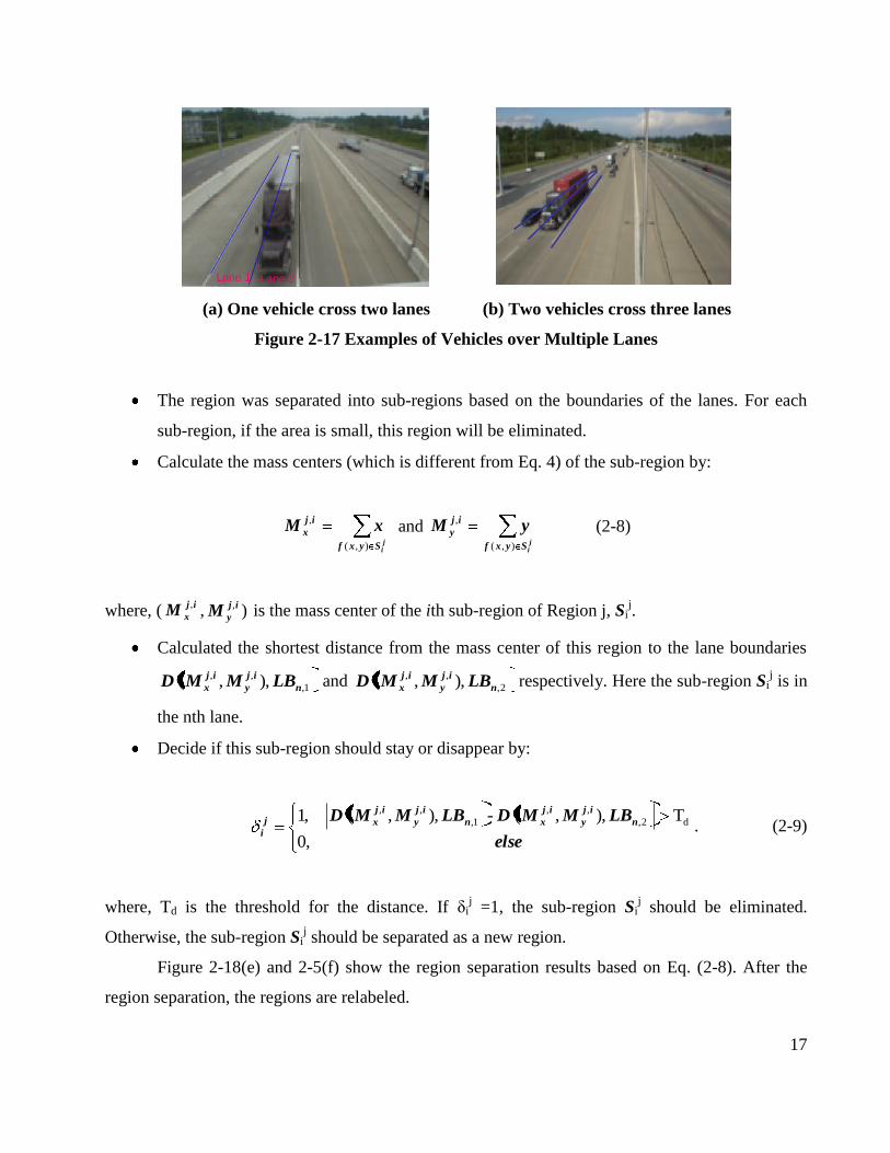
17

(a) One vehicle cross two lanes (b) Two vehicles cross three lanes

Figure 2-17 Examples of Vehicles over Multiple Lanes

The region was separated into sub-regions based on the boundaries of the lanes. For each

sub-region, if the area is small, this region will be eliminated.

Calculate the mass centers (which is different from Eq. 4) of the sub-region by:

jiSyxf

ij

x xM),(

, and

jiSyxf

ij

y yM),(

, (2-8)

where, (ij

xM,

, ),ij

yM is the mass center of the ith sub-region of Region j, Sij.

Calculated the shortest distance from the mass center of this region to the lane boundaries

1,

,, ),,( n

ij

y

ij

x LBMMD and 2,

,, ),,( n

ij

y

ij

x LBMMD respectively. Here the sub-region Sij is in

the nth lane.

Decide if this sub-region should stay or disappear by:

else

LBMMDLBMMD n

ij

y

ij

xn

ij

y

ij

xj

i,0

T ),,(-),,(,1 d2,

,,

1,

,,

. (2-9)

where, Td is the threshold for the distance. If δij =1, the sub-region Si

j

should be eliminated.

Otherwise, the sub-region Sij

should be separated as a new region.

Figure 2-18(e) and 2-5(f) show the region separation results based on Eq. (2-8). After the

region separation, the regions are relabeled.

Lane 1 Lane 2Lane 1 Lane 2

18

(a) Original

(b) Downsampled

(c) Calculated

Background Image

d) Subtraction of

Background Image

e) Threshold of

Subtraction Frame

f) Cleaned Threshold

g) Adjacent Cars

Separation

h) Joined Regions (Final Segmentation Results)

Figure 2-18 Illustration of the Separation Process

19

(e) Reconnect the Regions. After region separation, it is needed to check if there are regions

that satisfy the three rules in the section of Content-Based Region Connection, and connect those

regions.

(f) Dynamic Region Tracking. In this step, it is to find the moving direction of the regions

by finding the related location of in two consecutive video frames. If the entire region areas are used

to track the vehicle, there will be more computation complexity. Moreover, lane changing, or other

abnormal traffic patterns can be miss-identified. In this study, the center-tracking method was

employed.

If two regions from two consecutive video frames have certain a percentage of overlapping,

two regions are from same vehicle. Suppose 1i

nR and i

mR are from same vehicle. 1),( in

y

n

x CC and

im

y

m

x CC ),( are the centers for 1i

nR and i

mR respectively. The moving direction of the vehicle is

decided by the location of the centers. By tracking vehicle movement of initial video frames, the

traffic patterns can be determined for each lane.

Dynamic Vehicle Counting

To count the vehicle accurately, it is needed to avoid multiple counts of the same vehicle, or

miss-counting of any single vehicle. In real life, the patterns of the traffic may be abnormal, for

example, a vehicle may stop in the middle of driving for mechanical problems. Since, in this

system, our camera is setup to monitor the incoming or outgoing traffic, an invisible counting line is

initialized horizontally close the bottom of the video image. However, this invisible counting line

can be initialized vertically if the vehicles are in a side view.

Using the method described in the section of Dynamic Region Tracking, the movement of

the center can be monitored for each vehicle. For our cases, the camera is setup to take incoming or

outgoing patterns of the traffic. Only when the center of the vehicle passes the counting line in the

similar direction of a traffic patterns for that lane, the vehicle will be counted. To validate our

approach, a single video camera was set up on a tripod (6 feet high) on the cross bridge (Kessler

Ave.) over the interstate highway I-65 in Indianapolis, Indiana. The video frames are from both

incoming and outgoing traffics. The system was implemented on a dual Pentium 1.8G M laptop to

20

measure the accuracy of the system, two criteria that are commonly used to evaluate performance in

information retrieval are the precision rate and recall rates (18):

cars detected of No.

cars detectedcorrectly of No.rateprecision (2-10)

cars of No.

cars detectedcorrectly of No.rate recall (2-11)

The precision rate measures the percentage of the correctly detected and counted cars within

each video frames as opposed to detected cars, while the recall rate measures the percentage of

correctly detected cars that actually a cars. In 3000 video frames for incoming traffic and 3000

video frames for outgoing traffic. There are 70 cars for outgoing traffic, and 61 cars for incoming

traffic. For outgoing traffic, all 70 cars were correctly detected, but 6 cars have been counted twice.

For incoming traffic, 60 cars were correctly detected, but 2 cars have been counted twice. The

overall precision rate is 94.2%, and the recall rate is 99.2%. The experimental results demonstrate

the effectiveness of our system.

Dynamic Vehicle Classification

To make the system to be flexible, the users are allowed to setup the camera at wide range of

locations, heights, and angles. This created a great challenge in vehicle classification, where there is

no baseline about what the size and projection of a typical vehicle could be. In the literature,

researchers have used two approaches: using the parameters of the camera to accurately estimate the

projection and the size of vehicle; or use neural network approach for the training.

However, both approaches would not work in this project. In the first approach, to

accurately measure the parameters of the camera setting, the users need to have a lot of

measurements of the setup, including the height from the camera to the ground, the road curvature,

the tripod setup, the angle of the camera, the camera room ration, and the angle between the camera

to the vehicle when it proceeds in the scene. All of these are not only taking time, but also may not

be feasible. In the second approach, to use neural network, a lot of training would be necessary and

the accuracy may not be high (18).

21

In this study, the Maximum-likelihood approach was utilized for vehicle classification.

(a) Review of the Maximum-likelihood Method. The maximum-likelihood estimation

method has two advantages (19). First, it has very good convergence properties as the number of

training samples increases. Second, it is very simple in implementation and gives firm estimation.

Suppose that a collection of samples is separated according to class, the c data sets, cDD ,...,1 can be

determined with the samples in jD having been drawn independently according to the probability

law )|( jp x . There are several cases. When the samples behavior is unknown, the worst scenario

where samples are independent and identically distributed random variables (i.i.d), )|( jp x can be

assumed, and is therefore determined uniquely by the value of a parameter vector jθ .

Assume that the )|( jp x is Gaussian distribution: )|( jp x ~ ),( jjN μ , where jμ

represents the mean vector of the distribution of jθ , and j represents the variance vector of the

distribution. And jθ consists of the components of jμ and j . Since )|( jp x is independent of

jθ , )|( jp x can be rewritten as ),|( jjp θx . The goal is to use training samples to obtain good

estimates for the unknown parameter vectors cθθ ,...,1 . Suppose that D contains n samples nxx ,...,1 .

Because the samples were drawn independently, the following equation is obtained.

n

k

kpDp1

)|()|( θxθ . (2-12)

If )|( θDp is well-behaved, differential function of θ , θ̂ can be found by the standard

methods of differential calculus. If the parameters to be estimated is p, let θ denote the p-component

vector t),..., p1(θ , and θ be the gradient operator:

22

p

1

θ (2-13)

Defining )(θl as the log-likelihood function yields the following equation:

θ)θ |(ln)( Dpl (2-14)

The estimated θ̂ can be derived as:

)(ˆ θmax argθθ

l (2-15)

where, the dependence on the data set D is implicit. Plot Eq. (2-12) into Eq. (2-14) yields the

equations as follows:

n

k

pl1

|(ln)( θ)xθ k (2-16)

n

k

pl1

|(ln)( θ)xθ kθθ (2-17)

Thus, a set of necessary conditions for the maximum-likelihood for θ can be obtained from

the set of p equations.

0)(θθl (2-18)

A solution θ̂ to Eq. (2-18) could represent a true global maximum, a local maximum or

minimum, or (rarely) an inflection point of )(θl . Therefore, it is important to check if the extreme

occurs at a boundary of the parameter space, which might not be apparent from the solution. If all

solutions are found, it is guaranteed that one represents the true maximum.

23

(b) Data Training. In this study, the sample training is necessary. More training data can

help improve the recognition accuracy. However, it can take longer time. In a real-time setting,

more training could mean loose more data.

In this study, a quick training method that can be performed as little as 2000 frames (about 1

minute) training was proposed. The users can also change the number of training frames according

to their needs. When the unknown size vehicle passes by, the system will ask the users to input the

vehicle class. And the system will use the maximum likelihood estimation method introduced in the

section, Review of the Maximum-likelihood Method, to train the system. The value of this type of

vehicle will be updated and listed in the software for the users to review.

Occasionally, the segmentation may not be correct due to the quality of the image. As a

result, the trained result may not be correct. The proposed system allow the users to correct the

numbers based their experience.

(c) Image Projection and Size Correction Using Projection Geometrics. When acquiring

the image, due to the angle of the camera, the lane sizes are usually non-uniform in the image. The

vehicles (3D objects) are projected into 2-D plane (images). Many researchers have tried to model

the 3D objects from the 2D image. Some of them used multiple cameras, and some of them used

quite complicated math functions. These approaches not only made the system unnecessarily

complicated, but also have to have a lot of ideal assumption which would not work at all in real-life

scenario.

Figure 2-19 gives a demonstration of how image acquisition process becomes the projection

process. As a result, the center lanes tend to be wider than the side lanes in an image (if the camera

is focused on the center lanes). Also, the road closer to the camera are usually much wider than the

road further way. All these would affect the actual size of the vehicle in the image. For vehicles, the

closer to the camera parts would look much bigger/wider than those of further way. It is important

to properly project the data in the right plane.

24

Figure 2-19 Demonstration of Object Projection from 3D to 2D (20)

In this study, the projective geometry method was used to project the vehicles into the

corrected plane. The challenging of the projection is that the object may be locally deformed. And

different locations of the same object may have their own projection metrics. In computer graphics,

one of the most common matrices used for projection is 6=tuple, (left, right, bottom, top, near, far),

which defines the clipping planes. These planes form a box with the minimum corner at (left,

bottom, near), and the maximum corner at (right, top, far). The box is translated by:

(2-19)

It can also be given as a translation followed by a scaling of the form:

(2-20)

http://upload.wikimedia.org/wikipedia/commons/4/48/Axonometric_projection.svg

25

However, in this study, it was unable to get the three dimensional parameters from the 2D

image. It is ill-posed to model an 3D object by 2D image. Fortunately, only the size information

from the vehicle is needed for classification purpose. In this study, instead of modeling the

projection process as a 3D object to a 2D object, it was proposed to model the projection process as

from 2D plane to another 2D plane. It was assumed that the original 2D plane has corrected ration

of the vehicles in the lane, while the observed image was the projected result. Figure 2-20 demos

our linear projection idea. In this way, it becomes a linear projective geometry question to estimate

the correct vehicle sizes for classification. Here RP plane assumes to be the correct sized vehicle

plane, pp plane is the observed image plane. Since it is from 2D to another 2D plane, the parameters

can be easily and accurately estimated.

Figure 2-20 Linear Projective Geometry, Image from (21)

The following is a brief introduction of Projective Geometry.

26

Figure 2-21 Fundamental Theorem of Similarity, Image from (21)

The fundamental theorem of similarity (Figure 2-21) is used in this project to vehicle

projection transformation. In this theorem, it is a fact that for a triangle ABC, with line segment DE

parallel to side AB:

CD/DA = CE/EB. (2-21)

Figure 2-22 Parallel Lines in Projective Planes (Menelaus’s Theorem), Image from (21)

27

Figure 2-23 Cross Ratio, Image from (21)

Now in the plane situation (Figure 2-22), it is noted that A’B’ and D’E’ are not parallel; i.e.

the angles are not preserved. From the point of view of the projection, the parallel lines AB and DE

appear to converge at the horizon, or at infinity, whose project in the picture plane is labeled .

With the introduction of , the projected figure corresponds to a theorem discovered by Menelaus:

C’D’/D’A’ = C’E’/E’B’ B’/ A’ (2-22)

The cross ratio given four distinct collinear points A, B, C, D (Figure 2-23), the cross ratio is

defined as:

CRat(A,B,C,D) = AC/BC BD/AD (2-23)

Or CRat(A,B,C,D) = AC/BC AD/BD (2-24)

Eq. (2-24) reveals the cross ratio as a ratio of ratios of distances. Pappus proved that the

startling fact that the cross ratio was invariant, even though neither distance nor the ratio of distance

is preserved under projection:

CRat(A,B,C,D) = CRat(A’,B’,C’,D’) (2-25)

28

In this project, Eq. (2-25) and Eq. (2-21) were used to correctly estimate the vehicle size in a

corrected plane. Please note: this plane does not exist in the image, but it is mathematically used to

correct the ratio of the vehicle.

Shadow Reduction

Shadows (Figure 2-24) are determined based on three criteria; average color of the cluster,

cluster location relative to a cluster in an adjacent lane, and the shadow probability for that

particular lane. A shadow is defined as an adjacent cluster whose average color is less than 105.

For a given training period, the number of potential shadows is counted. Once the training period

expires, and a potential shadow is detected, one of two clusters could potentially be the shadow. If

both clusters are dark in color, the cluster with the higher probability is determined to be the shadow

and is removed from the difference frame. Figure 2-25 provides the flow chart for the shadow

detection algorithm.

Figure 2-24 Example of a Video Frame with Shadow

29

average color of

adjacent cluster <=

105?

Remove shadow

Is the shadow prob >

shadow prob of adjacent

cluster?

YES

YES

Update shadow

prob.

Check next lane

Average color of cluster

<= 105

adjacent cluster similar

in size and location?

YES

NO

YES

Figure 2-25 Shadow Removal Algorithm

As expected, the mean shift algorithm is too computationally expensive for a real-time

system. As a trivial case, an example image was created with clearly defined boundaries. The

mean shift clustering algorithm was successfully used to determine the boundaries, but took several

seconds to process the trivial image. Although the results were favorable, such a large processing

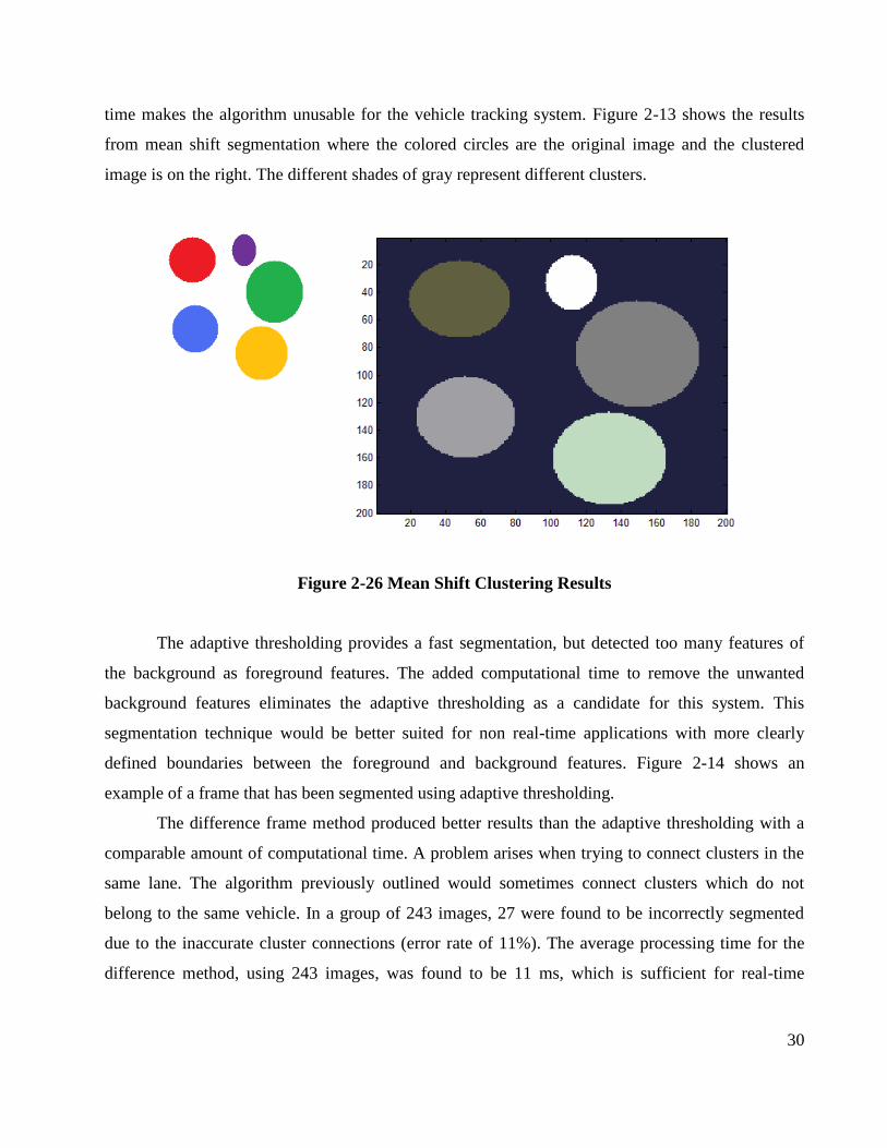
30

time makes the algorithm unusable for the vehicle tracking system. Figure 2-13 shows the results

from mean shift segmentation where the colored circles are the original image and the clustered

image is on the right. The different shades of gray represent different clusters.

Figure 2-26 Mean Shift Clustering Results

The adaptive thresholding provides a fast segmentation, but detected too many features of

the background as foreground features. The added computational time to remove the unwanted

background features eliminates the adaptive thresholding as a candidate for this system. This

segmentation technique would be better suited for non real-time applications with more clearly

defined boundaries between the foreground and background features. Figure 2-14 shows an

example of a frame that has been segmented using adaptive thresholding.

The difference frame method produced better results than the adaptive thresholding with a

comparable amount of computational time. A problem arises when trying to connect clusters in the

same lane. The algorithm previously outlined would sometimes connect clusters which do not

belong to the same vehicle. In a group of 243 images, 27 were found to be incorrectly segmented

due to the inaccurate cluster connections (error rate of 11%). The average processing time for the

difference method, using 243 images, was found to be 11 ms, which is sufficient for real-time

31

processing, but the error rate of 11% is too high. Figure 2-15 shows the incorrect connections

between clusters while Figure 2-16 gives an example of a correct connection using the difference

frame method.

Figure 2-14 Adaptive Thresholding Result

Figure 2-15 Incorrect Cluster Connection

Figure 2-16 Correct Cluster Connection

The shadow detection and removal algorithm has provided promising results. Of the 154

images tested, only 6 shadows were left unresolved, giving a preliminary success rate of 96%, with

an average computational time of 13 ms. Although the results are promising, the tests conducted

were with still images and further testing must be completed using the real-time system. Also, the

only test data available included a two lane road and for completeness, the algorithm needs to be

32

tested with three or more lanes. Figure 2-17 illustrates results of a successful shadow removal

scenario.

Figure 2-17 Results from the Shadow Detection and Removal Algorithm

In summary, several segmentation methods were studied in an attempt to find an alternative

method for a real-time vehicle counting and classification system. The mean shift clustering

algorithm has shown promising accuracy, but is computationally expensive and is therefore not best

suited for this system. The adaptive thresholding technique is fast, but the segmentation results are

highly inaccurate. The difference frame method has the best combination of accuracy and

computation time, but requires the use of an algorithm to connect neighboring clusters. The

connection algorithm provides inaccuracies in the final segmentation by connecting clusters which

do not belong to the same vehicle. In the end, it is determined that the current segmentation system

provides a better balance of accuracy and speed as compared to the three methods attempted. In

addition to investigating segmentation techniques, an algorithm was developed to detect and remove

unwanted shadows in the real-time system. The preliminary results show promise and thus

prompting the integration into the real-time system.

The Video Image Processing System

In order to validate the unclassified vehicle data associated with WIM vehicle classification

using automatic vehicle classification with video, a video image processing system as shown in

33

Figure 2-18 was developed using the dynamic content-based vehicle tracking and traffic monitoring

algorithms. In this study, a camcorder, DCR-SR100 30GB Handycam® CamcorderDCR-SR100,

was used to record the video vehicle data onto a VHS tape at the selected WIM sites.

The step-by-step instruction to use this system is provided in Appendix I.

Figure 2-18 Full View of the Software

34

Chapter 3

VALIDATION OF WIM VEHICLE CLASSIFICATION DATA USING VIDEO COUNTS

WIM Vehicle Classification Data

Potential Errors Associated with WIM vehicle Classification

For vehicle classification at a WIM site, sensors are placed in pavement to detect the arrival

of vehicle axles and generate correspondent signals. The signals are processed to determine vehicle

sizes and axle configurations to identify vehicle classes with a specific algorithm. Therefore, the

accuracy of vehicle classification depends on the sensitivity of sensors, environments, and road

conditions such as the number of lanes and traffic characteristics. Two types of errors may arise in

WIM vehicle classifications. First, data are missing from a particular WIM lane or all WIM lanes

(22). Data missing from all lanes is probably due to a system failure. However, data missing from a

particular lane is probably due to a lane closure or a sensor malfunction.

The second type of vehicle classification errors is that vehicles may not be classified. When

a vehicle executes lane changing on a multi-lane road, it is possible that only part of the vehicle

crosses the sensors. Vehicles may also accelerate or decelerate over the sensor, resulting in a speed

variation over the sensor. Additionally, different sensors may use different classification algorithms

that are not a pure science. As a result, errors may be involved in vehicle classifications. Because

missing data can be easily identified from WIM reports and because vehicle unclassification may be

involved at every WIM site, the validation of WIM classification focused on vehicle

unclassification.

WIM Classification Data

There are forty seven WIM sites on the highways under INTOT jurisdiction, thirty one sites

on interstate highways, and sixteen sites on US highways and State roads. The selection of WIM

sites for examining vehicle classifications was made mainly by taking into account those factors

affecting vehicle classifications, in particular number of lanes, traffic volume, and truck volume. In

35

addition, the ground conditions at the WIM sites should be suitable for safely setting up a camera

tripod to record quality video tapes of traffic at a certain angle. Presented in Table 3-1 is the data on

vehicle counts and unclassified vehicles at the selected eighteen WIM sites.

Table 3-1 WIM Vehicle Classification Data at Selected WIM Sites

WIM Site Info Traffic Counts Unclass.

(%) Site Road Dir. Lanes Vehicle Category Total

Counts 1 2 3 4 Unclass.

2000 I69 NB 2 603 56 190 5 49 903 13.3

2000 I69 SB 2 457 197 16 0 311 981 50.6

2300 I69 SB 2 397 316 279 4 22 1018 4.2

3400 I65 NB 3 1734 208 142 6 333 2423 40.3

3400 I65 SB 3 1846 206 278 14 82 2426 10.1

3510 I465 NB 6 3709 358 410 7 142 4626 34.5

3530 I465 SB 6 4626 252 309 10 212 5409 23.5

3600 I70 EB 2 648 70 264 15 95 1092 16.3

3600 I70 WB 2 822 36 208 24 52 1142 8.6

3700 I70 EB 2 667 73 312 23 20 1095 3.8

3700 I70 WB 2 706 177 329 11 32 1255 4.9

4000 I80/94 EB 4 1273 160 861 9 67 2370 7.6

4000 I80/94 WB 4 1023 133 376 5 883 2420 87.5

4100 I65 NB 2 814 102 160 1 313 1390 44.9

4100 I65 SB 2 912 59 316 13 14 1314 2.1

4200 I65 NB 3 2714 121 371 7 53 3266 4.8

4210 I65 SB 3 2864 149 341 11 59 3424 5.3

4400 I80/94 EB 3 2042 176 901 18 57 3194 5.6

4400 I80/94 WB 3 1836 178 868 9 276 3167 23.2

5300 I74 EB 2 1129 130 148 4 16 1427 2.3

5300 I74 WB 2 549 43 95 0 7 694 2.7

5400 I64 EB 2 778 59 161 6 11 1015 2.1

5400 I64 WB 2 1195 103 185 2 25 1510 3.1

5500 I65 NB 3 1156 165 364 9 95 1789 15.8

5510 I65 SB 3 1500 143 359 15 48 2065 6.9

6100 I64 EB 2 504 39 164 2 12 721 3.0

6100 I64 WB 2 538 42 187 2 15 784 4.0

6200 I64 EB 2 520 40 128 2 21 711 5.4

36

Video Vehicle Classification Data

Video Traffic Data Acquisition

Two main concerns may arise during video traffic data recording. In reality, the workplace

is a temporary roadside work zone involving people and equipment. While most overpass bridges

are on low volume roads, temporary traffic control devices to delineate the workplace. As a general

rule of thumb (23, 24), it is necessary to ensure all people, recording system, and vehicles are

visible to motorists. Equipment should not be placed behind grades or curves where sight distance

may not be sufficient. The second concern is the quality of data. In order to record the vehicle data

in the whole site, the camcorder should be placed above the middle of the driveway and oriented

down at 30~45 degrees (Figure 3-1). Light condition requires the clear view of the scene and no

long shadow of the vehicle. The best recording time period is 11am-2pm. To ensure the

camcorder’s tolerance, temperature should be 32 to 95 oF.

Figure 3-1 Camcorder Setting

Video Classification Data

In this study, Video traffic data was collected in July-August, 2007. The video tapes of

traffic were recorded using a camcorder, DCR-SR100 30GB Handycam® CamcorderDCR-SR100.

The camera tripod was usually set up on overpass bridges or places with a relatively high elevation

above the road. During traffic data recording, the camera was pointed to the back end of the traffic

flow downstream so as to avoid possible intrusion to motorists. At most selected WIM site, the

traffic flows in both directions were recorded. Due to the limitation of the video tape length, only

one hour traffic data was recorded in each direction. Table 3-2 shows the vehicle classification data

collected at twenty WIM sites.

37

Table 3-2 Video Vehicle Classification Data at WIM Sites

WIM Sites Vehicle Category Total

Counts Site Road Dir. Lanes 1 2 3 4

1100 I-65 SB 2 436 159 187 30 812

1100 I-65 NB 2 939 167 177 0 1283

1300 I-70 WB 2 1090 80 368 29 1567

1300 I-70 EB 2 565 80 212 23 880

2000 I-69 NB 2 530 116 203 45 894

2000 I-69 SB 2 637 50 218 13 918

3400 I-65 NB 3 1630 143 286 19 2078

3400 I-65 SB 1 500 19 6 0 525

3400 I-65 SB 3 1818 189 289 12 2308

3600 I-70 EB 2 410 49 178 11 648

3600 I-70 WB 2 810 76 240 24 1150

3700 I-70 EB 2 803 99 290 12 1204

3700 I-70 WB 2 807 69 260 7 1143

4000 I-80/94 EB 3 1570 188 1050 17 2825

4010 I-80/94 WB 3 1171 123 1100 20 2414

4100 I-65 SB 2 732 88 180 23 1023

4100 I-65 NB 2 707 49 350 6 1112

4200 I-65 NB 3 2106 120 366 12 2604

4210 I-65 SB 3 2300 140 295 12 2747

4400 I-80/94 WB 3 1860 148 928 16 2952

4400 I-80/94 EB 3 1730 262 754 168 2914

4700 SR-49 NB 2 683 47 78 3 811

4700 SR-49 SB 2 1000 111 72 9 1192

5100 I-65 NB 2 952 81 226 5 1264

5100 I-65 SB 2 657 233 99 103 1092

5300 I-74 WB 2 458 21 165 9 653

5300 I-74 EB 2 460 39 158 1 658

5400 I-64 EB 2 632 107 57 9 805

5400 I-64 WB 2 1140 176 130 6 1452

5500 I-65 NB 4 1178 171 230 40 1619

5510 I-65 SB 4 2284 354 297 100 3035

6100 I-64 EB 2 470 48 141 2 661

6100 I-64 WB 2 545 40 176 3 764

6200 I-64 EB 2 505 36 152 2 695

6200 I-64 WB 2 450 48 153 7 658

38

Data Analysis

Tolerance for Unclassified Vehicle Counts

Three observations can be made by careful inspection of the data in Table 3-1. First, at WIM

Site 4000, the unclassified vehicles reached 87.5% of total vehicle counts in westbound. This is

extremely high and might be due to a sensor failure. This site consists of four lanes in each

direction. Further examination of the WIM report indicated that the data was missed for the left lane

in both directions. However, the adjacent lane in west bound did not exhibit an increased vehicle

counts. This implies that the missing data was probably due to a sensor malfunction. Other WIM

sites that might experience sensor problems are those where unclassified vehicles exceed 30% of

the total vehicle counts. The second observation is that traffic volume might also contribute to the

vehicle unclassification issue. Plotted in Figure 3-2 are the variations of unclassified vehicles (%)

with vehicle counts. Notice that the data for those WIM site that might experience sensor

malfunctions was not included.

Figure 3-2 Variations of Unclassified Vehicles with Traffic Volume

It is shown that while most WIM sites witnessed a traffic volume varying from 600 to 3000

vehicles per hour, it appears that the percentage of unclassified vehicles increases as vehicle counts

39

increases. In reality, it was hypothesized that as traffic volume increases, the interaction between

vehicles increases and more vehicles may execute lane changing and passing. The third observation

is that in general, the percentage of unclassified vehicles increases as the number of travel lanes

increases at the WIM site as shown in Figure 3-3. This is probably because at a WIM site with more

travel lanes, the possibility for vehicles to execute lane changing or passing increases. Therefore,

more vehicles may occupy the two adjacent lanes or change speeds at sensors, which leads to

greater percentages of unclassified vehicles.

Figure 3-3 Variations of Unclassified Vehicles with Number of Lanes

This project examined the vehicle counts and classification data lane by lane and eliminated

those WIM sites with suspicious vehicle count data. As shown in Table 3-3 are the summaries of

the percentages of unclassified vehicles in each WIM lane with verified data. Since the WIM sites

utilize various sensors and the number of lanes varies from site to site, it is difficult to determine

specific bounds for estimating the percentage of unclassified vehicles at each WIM site. Based on

the unclassified vehicle data in Table 3-3, however, it appears that unacceptable errors may be

involved in the vehicle classification when the percentage of unclassified vehicles for a single lane

40

exceeds 4% of the total vehicle counts in that lane at a confidence level of 95%. In other words, it is

not acceptable when the percentage of unclassified vehicles exceeds 4% for a single lane.

Table 3-3 Summaries of Percentages of Unclassified Vehicles for Each WIM Lane

WIM

Site

Lane

ID

Unclass. (%)

WIM

Site

Lane

ID

Unclass. (%)

WIM

Site Lane ID

Unclass. (%)

2000 NB-#1 2.56 3600 WB-#3 5.34 4400 WB-#2 18.36

2000 NB-#2 10.69 3600 WB-#4 3.25 4400 WB-#3 1.91

2000 SB-#4 5.07 3700 EB-#1 1.72 5300 EB-#1 0.78

2300 SB-#1 2.38 3700 EB-#2 2.06 5300 EB-#2 1.51

2300 SB-#2 1.8 3700 WB-#3 3.03 5300 WB-#3 0.22

3400 NB-#2 2.51 3700 WB-#4 1.89 5300 WB-#4 2.44

3400 NB-#3 0.56 4000 EB-#1 1.34 5400 EB-#1 1.19

3400 SB-#4 5.62 4000 EB-#2 2.49 5400 EB-#2 0.88

3400 SB-#5 2.19 4000 EB-#3 3.75 5400 WB-#3 2.24

3400 SB-#6 2.31 4010 WB-#5 2.71 5400 WB-#4 0.9

3500 NB-#1 21.19 4010 WB-#6 3.35 5500 NB-#1 5.18

3500 NB-#2 2.92 4100 NB-#2 0.58 5500 NB-#2 6.35

3500 NB-#3 3.42 4100 SB-#1 1.15 5500 NB-#3 4.24

3510 NB-#4 2.23 4100 SB-#2 0.97 5510 SB-#4 1.33

3510 NB-#5 2.06 4200 NB-#1 1.05 5510 SB-#5 3.35

3510 NB-#6 2.63 4200 NB-#2 2.12 5510 SB-#6 2.19

3520 SB-#1 6.28 4200 NB-#3 1.67 6100 EB-#1 1.8

3520 SB-#2 3.42 4210 SB-#4 1.35 6100 EB-#2 1.2

3520 SB-#3 3.66 4210 SB-#5 2.87 6100 WB-#3 1.8

3530 SB-#4 3.98 4210 SB-#6 1.05 6100 WB-#4 2.2

3530 SB-#5 3.61 4400 EB-#4 2.6 6200 EB-#1 3.11

3530 SB-#6 2.51 4400 EB-#5 2.78 6200 EB-#2 2.27

3600 EB-#1 11.09 4400 EB-#6 0.25

3600 EB-#2 5.19 4400 WB-#1 2.89

Adjustment of Unclassified Vehicle Counts

In order to identify the compositions of unclassified vehicle counts at WIM sites, the video

vehicle counts presented in Table 3-2 are employed to validate the WIM vehicle counts.

Comparison can be made on the total WIM vehicle counts and the total video vehicle counts in each

direction at the WIM site as illustrated in Figure 3-4. In general, both the WIM vehicle counts and

the video vehicle counts follow a similar trend. However, great discrepancies can be observed at

41

some WIM sites, such as Sites 4200, 4210, 5510 SB, and 5300 WB. There are two possible

contributing factors. First, it is very difficult to exactly match the time period for WIM vehicle

counting to the time period for video vehicle counting. Any discrepancy between counting time

periods may lead to a large discrepancy between vehicle counts. Second, errors may be involved in

the unclassified vehicle count. It is possible that two or more vehicles might be counted as one

unclassified vehicle.

Figure 3-4 Comparison of WIM and Video Vehicle Counts

Therefore, the validation of unclassified vehicle counts was made by comparing the vehicle

category distributions in WIM and video vehicle counts, rather than the vehicle counts. The vehicle

category distribution is defined as the percentage of each vehicle category. Presented in Table 3-4

are the vehicle category distributions calculated from both the WIM and video vehicle counts.

Category 1, i.e., passenger cars, accounts for the greatest percentage of the total vehicle counts,

followed by Category 3, i.e., single tractor trailers, which accounts for up to 37% of the total vehicle

counts. Single unit trucks are the third largest category and account for 10% at most WIM sites.

Multi-trailer trucks under Category 4 account for the least percentage of the total vehicle counts,

which is less than 3% at most WIM sites.

41

Table 3-4 Comparison of Vehicle Category Distributions

WIM Site Information WIM Vehicle Category Distribution Video Vehicle category Distribution

Site Road Dir. Lanes 1 2 3 4 Unclass. Sum 1 2 3 4 Sum

2000 I69 NB 2 66.8 6.2 21.0 0.6 5.4 903 59.3 13.0 22.7 5.0 894

2000 I69 SB 2 46.6 20.1 1.6 0.0 31.7 981 69.4 5.4 23.7 1.4 918

3400 I65 NB 3 71.6 8.6 5.9 0.2 13.7 2423 78.4 6.9 13.8 0.9 2078

3400 I65 SB 3 76.1 8.5 11.5 0.6 3.4 2426 78.8 8.2 12.5 0.5 2308

3600 I70 EB 2 59.3 6.4 24.2 1.4 8.7 1092 63.3 7.6 27.5 1.7 648

3600 I70 WB 2 72.0 3.2 18.2 2.1 4.6 1142 70.4 6.6 20.9 2.1 1150

3700 I70 EB 2 60.9 6.7 28.5 2.1 1.8 1095 66.7 8.2 24.1 1.0 1204

3700 I70 WB 2 56.3 14.1 26.2 0.9 2.5 1255 70.6 6.0 22.7 0.6 1143

4000 I80/94 EB 4 53.7 6.8 36.3 0.4 2.8 2370 55.6 6.7 37.2 0.6 2825

4000 I80/94 WB 4 42.3 5.5 15.5 0.2 36.5 2420 48.5 5.1 45.6 0.8 2414

4100 I65 NB 2 58.6 7.3 11.5 0.1 22.5 1390 71.6 8.6 17.6 2.2 1023

4100 I65 SB 2 69.4 4.5 24.0 1.0 1.1 1314 63.6 4.4 31.5 0.5 1112

4200 I65 NB 3 83.1 3.7 11.4 0.2 1.6 3266 80.9 4.6 14.1 0.5 2604

4210 I65 SB 3 83.6 4.4 10.0 0.3 1.7 3424 83.7 5.1 10.7 0.4 2747

4400 I80/94 EB 3 63.9 5.5 28.2 0.6 1.8 3194 63.0 5.0 31.4 0.5 2952

4400 I80/94 WB 3 58.0 5.6 27.4 0.3 8.7 3167 59.4 9.0 25.9 5.8 2914

5300 I74 EB 2 79.1 9.1 10.4 0.3 1.1 1427 70.1 3.2 25.3 1.4 653

5300 I74 WB 2 79.1 6.2 13.7 0.0 1.0 694 69.9 5.9 24.0 0.2 658

5400 I64 EB 2 76.7 5.8 15.9 0.6 1.1 1015 78.5 13.3 7.1 1.1 805

5400 I64 WB 2 79.1 6.8 12.3 0.1 1.7 1510 78.5 12.1 9.0 0.4 1452

5500 I65 NB 3 64.6 9.2 20.3 0.5 5.3 1789 72.8 10.6 14.2 2.5 1619

5510 I65 SB 3 72.6 6.9 17.4 0.7 2.3 2065 75.3 11.7 9.8 3.3 3035

6100 I64 EB 2 69.9 5.4 22.7 0.3 1.7 721 71.1 7.3 21.3 0.3 661

6100 I64 WB 2 68.6 5.4 23.9 0.3 1.9 784 71.3 5.2 23.0 0.4 764

6200 I64 EB 2 73.1 5.6 18.0 0.3 3.0 711 72.7 5.2 21.9 0.3 658

42

The concerns on the unclassified vehicle counts have been raised by some researchers (25).

Since the vehicle classification data has been widely used by transportation agencies, the

importance of the work on making corrections on the unclassified vehicle counts can never be

overestimated. It is shown that in Table 3-4, the greatest discrepancy between the WIM and video

vehicle category distributions arose from Category 3, followed by Category 1 regardless of the

number of lanes. This implies that the unclassified vehicles mainly involved single tractor trailers

and passenger cars. The least discrepancy was observed for Category 2, which indicates that single

unit trucks were most likely classified. While traffic volume and lane number are the two main

contributing factors, it is unrealistic to predict the unclassified vehicles in terms of traffic volume

and lane number at this time. However, the adjustment factors in Table 3-5 can be utilized to

allocate the unclassified vehicles when it is needed. These factors are determined from the data in

Table 3-4 and represent the percentages of the unclassified vehicles for the four vehicle categories,

respectively.

Table 3-5 Adjustment Factors of Unclassified Vehicles

Vehicle Category 1 2 3 4

Adjustment Factors, % 35.0 5.0 48.0 12.0

43

Chapter 4

EVALUATION OF TIRTL’S FIELD PERFORMANCE

The TIRTL Vehicle Data Collection

One TIRTL system was installed to collect vehicle count and classification data by this

study as shown in Figure 4-1. The installation site is located at milepost 177.43 on I-65 in Lafayette,

Indiana, and is approximately 1.49 miles north of a weigh-in-motion (WIM) site on I-65. No any

access exists between the TIRTL site and the WIM site. Figure 4-2 shows a graphical illustration of

the locations of the TIRTL and WIM sites. There are four lanes at this site, two in each direction.

The installation of TIRTL was fully completed in April, 2008. The transmitter is placed southbound

and the receiver northbound. Both the transmitter and receiver are placed on a wood pole (see

Figure 4-1), respectively, so as to avoid possible blocking of the light beam pathways by ground

grasses or other obstacles in the median. The lane configuration at the TIRTL site is shown in

Figure 4-3. The driving and passing lanes in the northbound are designated as Lane 1 and Lane 2

with negatively signed velocities, respectively. In the southbound, the driving and passing lanes are

designated as Lane 4 and Lane 3 with positively signed velocities, respectively.

Figure 4-1 TIRTL System Installed on I-65 in Lafayette, IN

44

Figure 4-2 Graphical Illustration of TIRTL and WIM Sites

Figure 4-3 Lane Configuration

Three main files, including vehicle log file, system log file, and alarm log file can be

downloaded with point to point protocol connection. The vehicle log file records vehicle data,

including date, time, lane, velocity, and class number, axle count, wheel base, and class name. The

vehicle classification is based on the so-called “Scheme F”, in which, vehicles are classified into 15

categories. Categories 1 to 13 are as defined in Figure 2-1 in Chapter 2. Category 14 includes the

special vehicles defined by DOT personnel. Category 15 includes those vehicles which do not

confirm to the classification criteria for Class 1 through Class 14. The system log file is used to

record all activities, including internal maintenance and development support.

45

The alarm log data includes date, time, alarm name, and channels. There are three main

types of alarm, such as Beams Blocked, Beam Levels Degraded, and Beams Not Aligned. “Beams

Blocked” simply indicates the beams are totally blocked due probably to an obstruction such as a

vehicle parked front of the TIRTL system. “Beam Levels Degraded” implies that the generated

bema light may experience the loss of lumens due to surrounding factors such as fog. If this occurs,

however, the system may still perform well. “Beams Not Aligned” indicates that the beams are not

traveling directly between the transmitter and receiver. This may occur during set up, and may also

occur if the system cabinet is twisted.

Validation of TIRTL Data Accuracy by Manual Vehicle Counts

This study employed a manual vehicle count to validate the accuracy of the TIRTL vehicle

classification data since the manual count usually represents the baseline in many circumstances.

The manual vehicle count was conducted in the northbound direction on the Swisher Road overpass

bridge that is located immediately upstream of the TIRTL site on November 2, 2009. It was clear,

sunny. In order to reduce possible errors, the manual vehicle counting was made by two persons,

one person for the passing lane and the other for the driving lane. Since the traffic volume was

relatively high, the manual vehicle counting was made for one hour (9:10 am–10:10 am) in terms of

four vehicle categories as defined in Table 2-1. Table 4-1 shows the detailed manual and TIRTL

vehicle counts.

Table 4-1 Comparison of Manual and TIRTL Vehicle Counts

Vehicle

Category

Manual Count TIRTLE Count P. E.

Driving

Lane

Passing

Lane

Driving

Lane

Passing

Lane

Driving

Lane

Passing

Lane

1 291 241 295 240 1.4% 0.4%

2 38 1 32 0 15.8% 100.0%

3 237 38 244 36 3.0% 5.3%

4 10 1 9 1 10.0% 0%

Sub-Total 576 281 580 277 0.7 1.42

Total 857 857 0%

46

In order to measure the accuracy of the TIRTL vehicle count, the percent error used

elsewhere (26) is employed by this study to quantify the potential errors associated with the TIRTL

vehicle count. The calculation of the percent error depends on the baseline vehicle count. In this

case, the percent error is computed as follows:

(4-1)

where, P.E. is the percent error, the baseline count represents the manual vehicle count, and the

observed count represents the TIRTL vehicle count.

However, special care should be exercised when interpreting the percent errors, in particular

if the baseline count is low. This is because the percent error represents a relative error. When the

baseline count such as the manual count in Equation (4-1) is low, the calculated percent error may

be very high. As a result, the performance of the traffic counter may be exaggerated. It is shown that

the percent error for the total vehicle count in these two lanes is 0% and both the total manual

vehicle count and the total TIRTL vehicle count are 857 vehicles, respectively. The percent error for

the sub-total vehicle count in each lane is 0.7% for the driving lane and 1.4% for the passing lane.

Apparently, the total TIRTL vehicle counts agree extremely well with the total manual vehicle

count. For vehicle category count (or classification count), the percent error for Category 2 in the

passing lane is 100% and 0% for Category 4 in the passing lane. However, this should be ignored

simply because the baseline count, i.e., the manual count, is only one.

A more meaningful comparison should focus on Category 1 and Category 3 that account for

approximately 94% of the total traffic volume. As demonstrated in Table 4-1, the percent error for

Category 1 is 0.4% in the passing lane and 1.4% in the driving lane. For category 3, the percent

error is 3.0% in the driving lane and 5.3% in the passing lane. The TIRTL vehicle category count

agrees well with the manual vehicle category count for both Category 1 and Category 3. It was

observed that during manual vehicle counting, the errors might arise due to two main factors. First,

some vehicles executed lane-changing before arriving at the TIRTL site. Second, pick-up trucks

towing trailers might be misclassified. The percent error for Category 3 is greater than that for

Category 1. This implies that for TIRTL, the accuracy of vehicle classification for passenger cars is

47

better that that for tractor trailers. This is similar to the finding for the vehicle classification by WIM

as shown in Table 3-5.

Comparison of TIRTL and WIM Vehicle Counts

The Accuracy of WIM Vehicle Counts

In many circumstances, it is extremely labor intensive or even impractical to conduct

manual vehicle counting, in particular on multi-lane interstate highways with high traffic volumes,

in adverse weathers or for long duration counting. Therefore, the WIM vehicle classification data

collected at the WIM site as shown in Figure 4-2 was employed to further evaluate the TIRTL

performance. The requirements for WIM performance can be found elsewhere (27). In this study,

video vehicle counts were used to double check the accuracy of the WIM vehicle counts. As

tabulated in Table 4-2 are the Video and WIM vehicle counts made on November 21, 2008. The

weather was clear.

Table 4-2 Comparison of Video and WIM Vehicle Counts

Vehicle

Category

Video Count WIM Count P. E.

NB SB NB SB NB SB

0 - - 12 73 - -

1 829 984 787 843 5.1% 14.3%

2 56 69 44 159 21.4% 130.4%

3 360 309 370 265 2.8% 14.2%

4 20 13 21 7 5.0% 46.2%

Total 1265 1375 1234 1347 2.5% 2.0%

The vehicle counts were made on the Swisher Road overpass bridge during a duration of one

hour from 11:13am to 12:13pm in the northbound, and from 13:03pm to 14:03pm in the

southbound. Since the Video and WIM sites are approximately one and half miles apart, Table 4-2

presents the total vehicle counts in direction instead of each individual lane because of the possible

lane changing by vehicles between the Video and WIM sites. Category 0 represents the unclassified

vehicles. It is shown that the total Video and WIM vehicle counts agree very well in both directions.

The percent error is 2.5% in the northbound and 2.0% in the southbound. The percent errors for

48

Category 2 and Category 4 are very large. However, the vehicles in these two categories account

only for about 6% of the total vehicles. This may not affect the overall performance of WIM vehicle

classification very much.

TIRTL and WIM Daily Vehicle Class Counts

In order to make the comparison analysis more reliable, this study examined the vehicle

counts made by WIM and TIRTL during a duration of 24 hours. Presented in Table 4-3 are the daily

vehicle class counts made by WIM and TIRTL on five individual days, including three days in 2008

and two days in 2009. Class 0 represents those vehicles that could not be classified by WIM. For

TIRTL, Class 0 represents those vehicles under Class 14 and Class 15. Also presented in Table 4-3

are the percent errors (P.E.) between the WIM and TIRTL daily vehicle counts, and other

information such as average speed (V) and weather conditions.

Table 4-3 Comparison of WIM and TIRTL Daily Vehicle Class Counts

Vehicle Class

8/1/08 9/4/09 12/23/08 1/1/09 5/1/09

WIM TIRTLE WIM TIRTLE WIM TIRTLE WIM TIRTLE WIM TIRTLE

0 2282 1 7861 2 2517 3 712 0 680 2

1 502 975 115 782 118 511 98 41 82 245

2 20599 29897 9596 16577 10414 13690 10514 19035 24519 29233

3 16634 8825 10685 6088 11030 4319 9835 3905 12745 7623

4 270 721 215 564 145 440 56 70 215 313

5 4417 1386 3651 1386 2845 1030 2336 141 1474 1058

6 575 576 296 459 226 188 98 95 438 388

7 244 133 11 59 31 19 15 12 39 28

8 555 941 317 1073 283 562 104 112 478 1036

9 10054 9662 8166 10185 6704 4716 3072 3272 10048 7936

10 49 171 48 262 29 117 5 31 49 188

11 781 817 545 627 483 450 46 57 820 624

12 194 208 137 160 126 117 34 41 237 172

13 3 19 2 28 5 14 1 7 5 36

Total 57159 54332 41645 38252 34956 26176 26926 26819 51829 48882

P. E. 4.9% 8.1% 25.1% 0.4% 5.7&

V, mph 68 65 68 64 56 56 71 71 67 68

Weather Fog, Clear,

haze, Cloudy Rain, Overcast,

Cloudy, haze Overcast, Snow,

Freezing Rain Clear, Cloudy,

Overcast Rain, Overcast,

Cloudy

49

The total daily vehicle counts by TIRTL agree well with the total daily vehicle counts by

WIM, except December 23, 2008 when the percent error reached 25%. However, the overall

average speeds agree very well on December 23, 2008. While overcast, snow, and freezing rain

were observed on December 23, 2008, and while the average speeds reduced greatly, it remains

unclear, at this time, why the total daily vehicle counts by WIM and TIRTL differed greatly. The

unclassified vehicle count might be very large and become an issue associated with WIM vehicle

classification. Under Class 2 (passing cars), the vehicle class count by TIRTL is always greater than

that by WIM. Under Class 3 (van and pick-up truck), however, the vehicle class count by TIRTL is

always less than that by WIM. It was also observed that under Class 5 (single unit truck), the

vehicle class count by TIRTL is always much less than that by WIM.

The above observations confirm previous research findings reported elsewhere (28, 29),

which indicate that great discrepancies existed between the vehicle counts under Classes 2, 3 and 5

by TIRTL and other vehicle classifiers. To the authors’ knowledge, it appears that the vehicle

counts of Class 5 by TIRTL are more reasonable. This is because as shown in Tables 4-1 and 4-2,

the vehicles under Category 2 approximately account for 4.6% (manual counts) or 4.7% (video

counts) of the total vehicle counts. Since Category 2 consists of all vehicles under Classes 4, 5, 6,

and 7, the actual vehicle counts under Class 5 should be less than 4.6% or 4.7%. As shown in Table

4-3, Based on the vehicle counts in Table -4-3, the vehicle counts under Class 5 by WIM account

for 7.5% of the total vehicle counts by five-day average. However, the vehicle counts under Class 5

by TIRTL constitute 2.6% of the total vehicle counts by average.

Vehicle Class Distributions

In order to avoid possible concerns over the accuracy of WIM vehicle counts, this study

further computed the vehicle class distributions from the WIM and TIRTL vehicle class counts.

The vehicle class distribution is the variation of the percentages of vehicle class counts and

indicates how large one vehicle class count is in relative to the other vehicle class counts. At a

specific location on a certain road, the vehicle class distribution represents the relative values and

should not exhibit abrupt changes from time to time even though the total vehicle count may change

from time to time. In addition, the vehicle class distribution can find many applications in highway

50

project economic analysis, crash analysis, asset management, and pavement design. As presented in

Figure 4-4 are the vehicle class distributions computed from WIM and TIRTL vehicle counts,

respectively.

Figure 4-4 Vehicle Class Distributions by WIM and TIRTL

Apparently, discrepancies exist between the WIM and TIRTL vehicle class distributions.

First, the vehicle class distributions from TIRTL vehicle counts exhibit two outstanding peaks, one

at Class 2, and the other at Class 9. However, the vehicle class distributions from WIM vehicle

51

counts demonstrate more peaks and spread more evenly. Second, in the case of two-axle, four-tire

vehicles, i.e., all vehicles under Classes 2 and 3, the passenger cars (Class 2) are the dominant

vehicle type for TIRTL. Nevertheless, the other two-axle, four-tire vehicles, including pickups and

vane, may be more than the passenger cars for WIM. This implies that TIRTL may work better than

WIM to distinguish Class 3 from Class 2. Third, much more vehicles were classified as Class 5 by

WIM than by TIRTL.

The default truck class distributions (30) were also utilized to validate the TIRTL and WIM

vehicle class distributions. Figure 4-5 shows a comparison of vehicle class distributions among

TIRTL, WIM and other sources. TTC-1, TTC-2 and TTC-4 indicate the default truck class

distribution for major single-trailer truck routes under Type I, Type II, and Type III, respectively.

The truck class distribution for TIRTL or WIM is the average distribution determined from Figure

4-4. Again, the percentage of Class 5 by WIM is greater than those by TIRTL and default values.

Overall, the truck class distribution determined by TIRTL agrees with the default distributions

better than that by WIM. While it is difficult to confirm whether TIRTL or WIM provides better

performance, it appears that TIRTL can provide vehicle classification information with accuracy not

worse than WIM.

Figure 4-5 Comparison of Truck Class Distributions

52

Chapter 5

IMPACT OF WEATHER CONDITIONS ON TIRTL’S PERFORMANCE

The TIRTL System Operations

It is well known that the TIRTL system utilizes infra-red light technology to detect vehicle

information needed to count and classify passing vehicles. The detection method can be illustrated

using Figure 5-1 (31). When a TIRTL system is in operation, the transmitter emits two parallel and

two cross infra-red light beams that traverse across the roadway to the receiver on the opposite side

of the roadway. While a vehicle passing between the transmitter and receiver, each wheel interrupts

and breaks each of the four light beam pathways. Breaking of a light beam is called a Break Beam

Event. Re-establishment of the broken light beam’s continuity is called a Make Beam Event. The

receiver detects the precise time of each Beam Event. The speed is measured according to the

parallel beam breaking. The vehicle classification is performed on the basis of axle counts and inter-

axle spacings. The lane identification is accomplished on the basis of both parallel and cross beam

beaks.

Figure 5-1 Configuration of TIRTL Infra-Red Light Beams

It is highlighted that by the TIRTL vendor, the alignment of the transmitter and receiver

units plays a critical role. The beams traversing the roadway should be set at a point as low as

53

possible so as to reduce the interference from mud-flaps and other features hanging from the main

body of the vehicles. Since the accuracy of TIRTL system depends largely on the effective

detection of the Beam Events between the transmitter and receiver, any disturbance to the light

beams by objects other than passing wheels may degrade the system performance. In order to avoid

the disturbance to the light beams by vegetation in the median of roadway, the transmitter and

receiver can be placed above the pavement at a pre-determined height. However, the possible

disturbance to the light beams due to rain and snow remains unknown and needs to be further

investigated (28).

Impact of Weather Conditions

Clear Weather

In order to evaluate the potential impacts of adverse weathers on the TIRTL performance,

this study examined both TIRTL and WIM data under different weather conditions. Since no

manual vehicle counts were available, WIM data was considered as the baseline data. Presented in

Table 5-1 are the percent errors between the WIM and TIRTL vehicle counts for Classes 2, 3, 5, and

9 under clear weather conditions. Also presented in Table 5-1 are the percent errors between the

total vehicle counts for all 13 classes by WIM and TIRTL. The positive sign, “+”, indicates that the

TIRTL count is greater than the WIM count, and the negative sign, “-“, indicates that TIRTL count

is less than the WIM count. As anticipated, the greatest percent error occurred under Class 5,

followed by Class 2 and Class 3. Under a given vehicle class except for Class 3, the TIRTL counts

may greater or less than the WIM counts. This indicates that the percent errors are random numbers

in clear weather. However, the TIRTL counts is always less than WIM counts under Class 3

Table 5-1 Percent Errors in Clear Weather

Class 1/21/09 5/24/09 6/23/09 8/2/08 9/25/08

2 54.5(+) 29.4(+) 51.1(+) 71.7(+) 30.1(-)

3 46.4(-) 38.5(-) 14.7(-) 49.0(-) 69.5(-)

5 33.3(-) 121.7(+) 49.0(+) 81.8(-) 37.2(-)

9 1.2(-) 5.7(-) 39.1(-) 3.6(+) 63.2(-)

All Classes 0.3(-) 14.0(+) 30.7(+) 1.4(+) 45.6(-)

54

Adverse Weathers

Presented in Table 5-2 are the percent errors between the WIM and TIRTL counts under

foggy weather conditions. The greatest percent error arose under Class 2. Under Class 2, the TIRTL

counts are greater than the WIM counts. Under Classes 3 and 5, the TIRTL counts are less than the

WIM counts. Under Class 9, the TIRTL count is greater than the WIM count on August 6, 2008 and

less than the WIM count on January 4, 2009. It looks that the percent errors in foggy weather are

greater than those in clear weather. Under All Classes, however, the percent errors in foggy weather

are similar to those in clear weather in Table 5. Due to limited data, there is no evidence to indicate

the impact of foggy weather.

Table 5-2 Percent Errors in Foggy Weather

Class 8/6/08 1/4/9

2 124.5(+) 58.3(+)

3 4.5(-) 70.5(-)

5 82.8(-) 81.8(-)

9 13.7(+) 60.4(-)

All Classes 11.2(+) 39.1(-)

Table 5-3 shows the percent errors between TIRTL and WIM counts in normal snowy

weather. The TIRTL counts are greater the WIM counts under some classes, and less than the WIM

counts under other classes. No evidence is available to indicate the impact of snow. Again, the

TIRTL counts under Class 3 are less than the WIM counts. Tabulated in Table 5-4 are the percent

errors in wet weathers, such as normal rainy and thunderstorm weathers. In normal rainy weather,

the TIRTL counts are greater than the WIM counts in some cases, and less than the WIM counts in

other cases. As anticipated, the TIRTL counts are less than the WIM counts under Class 3. No

specific pattern can be identified in the variations of the percent errors.

In thunderstorm weather, the TIRTL counts are always less than the WIM counts regardless

of vehicle class and survey date. Compared to all other weathers, it looks that the percent errors in

thunderstorm weather are very large. Class 9 witnessed the greatest percent errors, followed by

Class 3. Even the overall percent errors for All Classes are very high and close to 95%. It can be

concluded that in thunderstorm weather, the TIRTL system may undercount vehicles. This agrees

55

with a finding by another study (28), which indicated that severe weather affects the TIRTL

sensor’s performance and causes traffic to be undercounted.

Table 5-3 Percent Errors in Normal Snowy Weather

Class 8/6/08 1/4/09

2 23.8(+) 72.9(+)

3 63.3(-) 45.1(-)

5 62.7(-) 76.6(-)

9 40.3(-) 6.2(+)

All Classes 42.3(-) 0.2(-)

Table 5-4 Percent Errors in Wet Weather

Class Normal Rainy Weather Thunderstorm Weather

8/23/08 9/4/08 5/1/09 6/18/09 3/13/09 5/15/09 6/1/09 8/5/08

2 57.4(+) 14.9(+) 0.7(-) 16.7(-) 88.9(-) 96.7(-) 27.1(-) 68.1(-)

3 48.7(-) 60.3(-) 47.2(-) 40.4(-) 92.7(-) 98.2(-) 54.3(-) 87.2(-)

5 22.7(-) 25.6(-) 23.7(+) 23.5(+) 81.6(-) 79.3(-) 40.8(-) 91.7(-)

9 12.8(-) 54.5(-) 80.8(-) 82.3(-) 100.0(-) 100.0(-) 61.9(-) 100.0(-)

All Classes 0.7(+) 27.8(+) 22.0(+) 36.1(+) 92.4(-) 94.9(-) 42.3(-) 87.5(-)

56

Chapter 6

CONCLUSIONS

Video Vehicle Detection and Classification

The digital image based vehicle monitoring and classification system developed by this

study is user friendly and can be easily to setup, and perform data acquisition, vehicle monitoring,

and length-based vehicle classification. This system can help develop the models for correcting

weigh-in-station data, in particular the unclassified vehicle counts. It was shown that the traditional

method to treat all unclassified vehicle counts as trucks is too conservative and will largely

overestimate the truck traffic volume. Video technologies can provide accurate and effective vehicle

detection when vehicles are classified into four categories, including two-axle, four-tire vehicles,

single unit trucks, single-trailer trucks, and multi-trailer trucks.

WIM Vehicle Detection and Classification

WIM sensor malfunction can generate serious vehicle classification issues. The percentage

of unclassified vehicles increases as vehicle counts increases. As the number of travel lanes

increases, the possibility for vehicles to execute lane changing or passing increases. Therefore, more

vehicles may occupy two adjacent lanes or change speeds on sensors, leading to greater percentages

of unclassified vehicles. It becomes unacceptable when the percentage of unclassified vehicles

exceeds 4% for a single lane.

Based on the WIM data statewide, the unclassified vehicles mainly involved single tractor

trailers and passenger cars. Single unit trucks were most likely classified by WIM. While traffic

volume and lane number are the two main contributing factors, it is unrealistic to predict the

unclassified vehicles in terms of traffic volume and lane number at this time. Overall, vehicles

under Categories 1, 2, 3, and 4 account respectively for 35%, 5%, 48%, and 12% of the total

unclassified vehicles.

57

TIRTL Vehicle Detection and Classification

Under clear weather conditions, the TIRTL vehicle counts agreed very well with the manual

and video vehicle counts, respectively. When vehicles are classified into four categories, such as

two-axle, four-tire vehicles, single unit trucks, single-trailer trucks, and multi-trailer trucks, the

accuracy of vehicle classification for Category 1, including all two-axle, four-tire vehicles, was

better than that for tractor trailers. WIM vehicle counts were utilized to validate the performance of

TIRTL system. Unlike WIM system, the number of unclassified vehicles by TIRTL was very small.

For axle-based vehicle classification, i.e., the 13-class FHWA vehicle classification scheme,

great discrepancies existed between the WIM and TIRTL vehicle class counts. Both WIM and

TIRTL demonstrated difficulties to distinguish Class 3 from Class 2. However, TIRTL

demonstrated better performance to identify vehicles under Class 3 than WIM, regardless of

weather conditions. Under Class 5, the TIRTL vehicle counts were more reasonable than the WIM

vehicle counts. The WIM system might over-count vehicles under Class 5. Based on the default

truck class distributions, TIRTL might provide vehicle classification more accurate than WIM.

Under normal weathers, fog, snow, and rain did not affect TIRTL’s performance. Under

thunderstorm weather, however, TIRTL might undercount vehicles regardless of vehicle class.

58

References

(1) Mechanistic-Empirical Pavement Design Guide, Interim Edition: A Manual of Practice Manual,

American Association of State Highway and Transportation Officials, Washington, DC, July,

2008.

(2) Office of Highway Policy Information, Traffic Monitoring Guide, Federal Highway

Administration, U.S. Department of Transportation, 2001.

(3) Shuo Li, Tommy Nantung, and Yi Jiang (2005). “Assessing issues, technologies, and data needs

to meet traffic input requirements by M-E pavement design guides: Implementation

Initiatives.” Transportation Research Record 1917, Journal of the Transportation Research

Board, 141-148.

(4) Andrew P. Nichols and Darcy M. Bullock, Quality Control Procedures for Weigh-in-Motion

Data, JTRP Preliminary Draft, Purdue University, 2004.

(5) TIRTLsoft V1.19 User Manual–Edition1.1.0, Control Specialists Company, Winter Park, FL

32789.

(6) D. Beymer, P. Mclauchlan, B. Coifman, and J. Malik (1997). “A real-time computer vision

system for measuring traffic parameters.” Proc. of IEEE Conf. Computer Vision and Pattern

Recotniion, 496-501.

(7) D. Koller, J. Weber, and J. Malik (1994). “Robust multiple car tracking with occlusion

reasoning.” Proc. of ECCV, 189-196.

(8) K. P. Karmann, and A. Von Brandt (1990). “Moving object recognition using an adaptive

background memory.” Proc. of Time-Varying Image Processing and Moving Object

Recognition, Vol. 2.

(9) O. Masoud, N.P. Papanikolopoulos, and N. Kwon (1997). “Vision-based monitoring of weaving

sections.” Proc. of IEEE Conf. Intelligent Transportation Systems, 338-343.

(10) S. Gupte, O. Masoud, R. F. K. Martine, and N. P. Papanikolopoulos (2002). “Detection and

Classification of Vehicles.” IEEE Transactions on Intelligent Transportation Systems, 3(1), 37-

47.

(11) B. Bhanu, S. Lee, and S. Das (1995). “Adaptive image segmentation using genetic and hybrid

search methods.” IEEE Trans. Aerosp. Electron. Syst., 31(4), 1268-1290.

59

(12) C.-S. Fuh, S.-W. Cho, and K. Essing (2000). “Hierarchical color image region segmentation

for content-based image retrieval system.” IEEE Trans. Image Processing, 9(1), 156-162.

(13) J. Chen, T.N. Pappas, A. Majsilovic, B.E. Rogowitz (2005). “Adaptive perceptual color-texture

image segmentation,” IEEE Trans. Image Processing, 14(10), 1524-1536.

(14) T. Gevers, “Image segmentation and similarity of color-texture objects (2002).” IEEE

Transactions on Multimedia, 4(4), 509-516.

(15) S. Sun, D. R. Haynor, Y. Kim (2003). “Semiautomatic video object segmentation using

vsnakes,” IEEE Trans. Circuits and Systems for Video Technology, 13(1).

(16) M. E. Farmer and A. K. Jain (2005). “A wrapper-based approach to image segmentation and

classification,” IEEE Trans. Image Processing, 14(12), 2060-2072, 2005.

(17) Design and Construction Reference Guide. Indiana Department of Transportation, 2007.

(18) Y. Du, C.I Chang, and P.D. Thouin (2003). "Automated system for text detection in individual

video Images.” Journal of Electronic Imaging, Vol. 12, No. 3, 410-422.

(19) R.O.Duda, P.E. Hart, and D.G. Stork, Pattern Classification, 2nd

Edition, Wiley Interscience:

New York, 2000.

(20) http://en.wikipedia.org/wiki/File:Axonometric_projection.svg.

(21) http://www.britannica.com/EBchecked/topic/478486/projective-geometry.

(22) Bill McCall, and W. C. Vodrazka, Jr. (1997). States’ Successful Practices Weigh-In-Motion

Handbook, CTRE, Iowa State University.

(23) Manual on Uniform Traffic Control Devices, 2003 Edition, Federal Highway Administration,

U.S. Department of Transportation.

(24) Best Practices Guidebook: Collecting Short Duration Manual Vehicle Classifications Counts

on Highway Volume Urban Facilities, Carter and Burgess, Inc., Denver, CO 80202, 2005.

(25) Nikiforos Stamatiadis and David L. Allen (1997). “Seasonal factors using vehicle classification

data.” Transportation Research Record 1593, Journal of the Transportation Research Board,

23-28.

(26) Battelle Memorial Institute (2004). Traffic Data Quality Measurement, Final Report. Work

Order Number BAT 03-007. 505 King Avenue, Columbus, Ohio 43201.

(27) ASTM Designation E 1318-02. Standard Specification for Highway Weigh-In-Motion (WIM)

Systems with User Requirements and Test Methods, ASTM 04.03.

http://en.wikipedia.org/wiki/File:Axonometric_projection.svg

http://www.britannica.com/EBchecked/topic/478486/projective-geometry

60

(28) Jerry Kotzenmacher, Erik Minge, and Bingwen Hao (2005). Evaluation of Portable Non-

Intrusive Traffic Detection System, Final Report, 2005-37, Minnesota Department of

Transportation.

(29) Xin Yu (2009). “Evaluation of non-intrusive sensors for vehicle classification on freeways.”

2nd

International Symposium on Freeway and Tollway Operations, June 21-24, 2009,

Honolulu, Hawaii.

(30) Guide for Mechanistic-Empirical Design of New and Rehabilitated Pavement Structures,

NCHRP 1-37A, Final Report, ERES Consultants Division, ARA Incorporation, March 2004.

(31) TIRTLsoft V1.19 for Windows: User Manual, Doc: TSUM 001, Edition: 1.1.0, CEOS

Industrial Pty. Ltd., Unit 3, 17 Burgundy Street, Heidelberg, Victoria, 3084, Australia.

site verification of weigh-in-motion traffic and tirtl

Documents