This article was downloaded by: [The University of Manchester Library]On: 26 October 2014, At: 16:24Publisher: Taylor & FrancisInforma Ltd Registered in England and Wales Registered Number:1072954 Registered office: Mortimer House, 37-41 Mortimer Street,London W1T 3JH, UK

International Journal ofMathematical Education inScience and TechnologyPublication details, including instructions forauthors and subscription information:http://www.tandfonline.com/loi/tmes20

Six ways to look at linearinterpolationAnwar H. JoarderPublished online: 11 Nov 2010.

To cite this article: Anwar H. Joarder (2001) Six ways to look at linearinterpolation, International Journal of Mathematical Education in Science andTechnology, 32:6, 932-937, DOI: 10.1080/002073901317147915

To link to this article: http://dx.doi.org/10.1080/002073901317147915

PLEASE SCROLL DOWN FOR ARTICLE

Taylor & Francis makes every effort to ensure the accuracy of allthe information (the “Content”) contained in the publications on ourplatform. However, Taylor & Francis, our agents, and our licensorsmake no representations or warranties whatsoever as to the accuracy,completeness, or suitability for any purpose of the Content. Any opinionsand views expressed in this publication are the opinions and views ofthe authors, and are not the views of or endorsed by Taylor & Francis.The accuracy of the Content should not be relied upon and should beindependently verified with primary sources of information. Taylor andFrancis shall not be liable for any losses, actions, claims, proceedings,demands, costs, expenses, damages, and other liabilities whatsoeveror howsoever caused arising directly or indirectly in connection with, inrelation to or arising out of the use of the Content.

This article may be used for research, teaching, and private studypurposes. Any substantial or systematic reproduction, redistribution,reselling, loan, sub-licensing, systematic supply, or distribution in anyform to anyone is expressly forbidden. Terms & Conditions of access

and use can be found at http://www.tandfonline.com/page/terms-and-conditions

Dow

nloa

ded

by [

The

Uni

vers

ity o

f M

anch

este

r L

ibra

ry]

at 1

6:24

26

Oct

ober

201

4

Six ways to look at linear interpolation

ANWAR H. JOARDER

Department of Mathematical Sciences, King Fahd University of Petroleum and Minerals,PO Box 1334, Dhahran 31261, Saudi Arabia

Email: anwarj@kfupm.edu.sa

(Received 30 November 2000)

Linear interpolation has been explained from di� erent perspectives that arelikely to be easily understood by students. Some methods seem to be moreinteresting in some situations. Apart from its suitability in classrooms, it hasalso a mnemonic value often expected by many readers.

1. Introduction

If a line is used to estimate a functional value between y-values for which the x-values are known, the process is called linear interpolation. In other words itconsists of putting a line through two points over small regions on a curve, andthen using the line to approximate the curve. Consider three points A…x1; y1†,C…x; y†, B…x2; y2† on a line where y is unknown and y1 < y < y2. Let us representthem by

x1 y1

x y

x2 y2

The value of y is obtained by equating slopes as follows:

y ¡ y1

x ¡ x1

ˆ y2 ¡ y1

x2 ¡ x1

…1†

which is popularly known as linear interpolation.In this note linear interpolation has been viewed in several ways. They have

been labelled as the ratio method, the distance method, the weighing method, thedeterminant method, the least squares method and the expected value method.They are also illustrated with examples. An application is shown to derive theformula for median in the context of a frequency distribution. Finally linearinterpolation has been characterized as the expected value of a random variablebased on a uniform probability distribution.

2. Some representations of linear interpolation

2.1. The ratio methodSince A, C and B are assumed to be on a line, it is easy to check that C divides

AB at the ratio

932 Classroom notes

Dow

nloa

ded

by [

The

Uni

vers

ity o

f M

anch

este

r L

ibra

ry]

at 1

6:24

26

Oct

ober

201

4

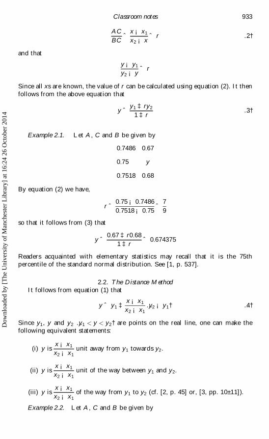
AC

BCˆ x ¡ x1

x2 ¡ xˆ r …2†

and that

y ¡ y1

y2 ¡ yˆ r

Since all xs are known, the value of r can be calculated using equation (2). It thenfollows from the above equation that

y ˆ y1 ‡ ry2

1 ‡ r…3†

Example 2.1. Let A, C and B be given by

0:7486 0:67

0:75 y

0:7518 0:68

By equation (2) we have,

r ˆ0:75 ¡ 0:7486

0:7518 ¡ 0:75ˆ

7

9

so that it follows from (3) that

y ˆ 0:67 ‡ r0:68

1 ‡ rˆ 0:674375

Readers acquainted with elementary statistics may recall that it is the 75thpercentile of the standard normal distribution. See [1, p. 537].

2.2. The Distance MethodIt follows from equation (1) that

y ˆ y1 ‡ x ¡ x1

x2 ¡ x1

…y2 ¡ y1† …4†

Since y1, y and y2 …y1 < y < y2† are points on the real line, one can make thefollowing equivalent statements:

(i) y isx ¡ x1

x2 ¡ x1

unit away from y1 towards y2.

(ii) y isx ¡ x1

x2 ¡ x1

unit of the way between y1 and y2.

(iii) y isx ¡ x1

x2 ¡ x1

of the way from y1 to y2 (cf. [2, p. 45] or, [3, pp. 10±11]).

Example 2.2. Let A, C and B be given by

Classroom notes 933

Dow

nloa

ded

by [

The

Uni

vers

ity o

f M

anch

este

r L

ibra

ry]

at 1

6:24

26

Oct

ober

201

4

0:9495 1:64

0:95 y

0:9505 1:65

Here

x ¡ x1

x2 ¡ x1

ˆ 0:0005

0:0010ˆ 0:5

so that y is 0.5 unit away from y1 towards y2. That is y ˆ 1:64 ‡ 0:5…1:65 ¡ 1:64† ˆ1:645. Readers acquainted with elementary statistics may recall that 1.645 is the95th percentile of the standard normal distribution. See [1, p. 537].

2.3. The weighing methodThe equation (1) can also be written as

y ˆ y1 ‡ x ¡ x1

x2 ¡ x1

y2 ¡ x ¡ x1

x2 ¡ x1

y1 ˆ …1 ¡ w†y1 ‡ wy2 …5†

where

w ˆx ¡ x1

x2 ¡ x1

If x1 < x < x2, then by subtracting x1 from both sides of x < x2, it follows that0 < w < 1. Similarly it can be proved that 0 < w < 1 if x1 > x > x2. Let us applythis method to Example 2.1 so that

w ˆ x ¡ x1

x2 ¡ x1

ˆ 0:75 ¡ 0:7486

0:7518 ¡ 0:7486ˆ 0:4375

which, by the distance method, means that y is 0.4375 unit away from y1 towardsy2. Clearly y is closer to y1 than it is to y2. By the weighing method we then have

y ˆ …1 ¡ w†y1 ‡ wy2 ˆ …1 ¡ 0:4375†y1 ‡ 0:4375y2

ˆ …0:5625†0:67 ‡ …0:4375†0:68 ˆ 0:674375

It may be remarked here that in many situations x2 ¡ x1 ˆ 1 so that w ˆ x ¡ x1. Inthose situations the weighing method is easily grasped by students. It is explainedbelow by an example.

Example 2.3. Consider a sample [1, p. 46] with n ˆ 10 observations with thesecond largest 5.4 and the third largest 5.7. The rank of the lower quartile …Q1† is…n ‡ 1†=4 ˆ …10 ‡ 1†=4 ˆ 2 ‡ 0:75 so that the lower quartile is an observationbetween the second and the third as depicted in the following table:

Rank Observation

2 5:4

2:75 Q1

3 5:7

934 Classroom notes

Dow

nloa

ded

by [

The

Uni

vers

ity o

f M

anch

este

r L

ibra

ry]

at 1

6:24

26

Oct

ober

201

4

Here w ˆ x ¡ x1 ˆ 2:75 ¡ 2 ˆ 0:75 so that it follows from (5) that

Q1 ˆ …1 ¡ 0:75† …second observation† ‡ 0:75 …third observation†

ˆ …1 ¡ 0:75†…5:4† ‡ 0:75…5:7† ˆ 5:625

It is interesting to note that the weights are intuitively appealing here. The rank2.75 of the lower quartile implies that it is closer to the 3rd observation than it is tothe second. So the weights 0.75 and 0.25 must be attached to the third and thesecond observations respectively. This type of problem is frequently encounteredin statistics and it seems this method is the best, especially in classrooms, forcalculating quartiles, deciles, percentiles or in general for quantiles.

2.4. The determinant methodSince the three points are on a line, the area of the triangle made by the three

points must vanish, hence in general we have

x1 y1 1

x y 1

x2 y2 1

­­­­­­­­­

­­­­­­­­­

ˆ 0 …6†

Those who are acquainted with determinants can easily evaluate that

x1…y ¡ y2† ¡ y1…x ¡ x2† ‡ …xy2 ¡ yx2† ˆ 0

Consider interpolating the value of y from Example 2.1. We have

0:7486 0:67 1

0:75 y 1

0:7518 0:68 1

­­­­­­­­­

­­­­­­­­­

ˆ 0

whence

0:7486…y ¡ 0:68† ¡ 0:67…0:75 ¡ 0:7518† ‡ 1‰0:75…0:68† ¡ 0:7518yŠ ˆ 0

and consequently, y ˆ 0:674375.

2.5. The least squares methodThe equation (1) can be written as

y ˆ ¡ x1y2 ¡ y1x2

x2 ¡ x1

‡ y2 ¡ y1

x2 ¡ x1

x …7†

But it is easy to check that the least squares estimates of ­ 0 and ­ 1 in the liney ˆ ­ 0 ‡ ­ 1x based on the points …x1; y1† and …x2; y2† are given by

­ 1 ˆ …x1 ¡ ·xx†…y1 ¡ ·yy† ‡ …x2 ¡ ·xx†…y2 ¡ ·yy†…x1 ¡ ·xx†2 ‡ …x2 ¡ ·xx†2

ˆ y2 ¡ y1

x2 ¡ x1

and

­ 0 ˆ ·yy ¡ ­ 1 ·xx ˆ y1x2 ¡ x1y2

x2 ¡ x1

Classroom notes 935

Dow

nloa

ded

by [

The

Uni

vers

ity o

f M

anch

este

r L

ibra

ry]

at 1

6:24

26

Oct

ober

201

4

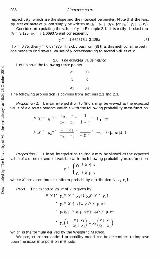
respectively, which are the slope and the intercept parameter. Note that the leastsquares estimate of ­ 0 can simply be written as ­ 0 ˆ y1 ¡ ­ 1x1 (or ­ 0 ˆ y2 ¡ ­ 1x2).

Consider interpolating the value of y in Example 2.1. It is easily checked that

­ 1 ˆ 3:125, ­ 0 ˆ ¡1:669375 and consequently

y ˆ ¡1:669375 ‡ 3:125x …8†

If x ˆ 0:75, then y ˆ 0:674375. It is obvious from (8) that this method is the best ifone needs to ®nd several values of y corresponding to several values of x.

2.6. The expected value methodLet us have the following three points

x1 y1

x c

x2 y2

The following proposition is obvious from sections 2.1 and 2.3.

Proposition 1. Linear interpolation to ®nd c may be viewed as the expectedvalue of a discrete random variable with the following probability mass function:

P …Y ˆ y1† ˆ x2 ¡ x

x2 ¡ x1

ˆ 1

1 ‡ rˆ 1 ¡ w

P …Y ˆ y2† ˆ x ¡ x1

x2 ¡ x1

ˆ r

r ‡ 1ˆ w; 0 µ w µ 1

Proposition 2. Linear interpolation to ®nd c may be viewed as the expectedvalue of a discrete random variable with the following probability mass function:

Y ˆy1 if X ¶ x

y2 if X µ x

(

where X has a continuous uniform probability distribution U…x1; x2†.

Proof. The expected value of y is given by

E…Y† ˆ y1P…Y ˆ y1† ‡ y2P…Y ˆ y2†

ˆ y1P…X ¶ x† ‡ y2P…X µ x†

ˆ y1‰1 ¡ P…X µ x†Š ‡ y2P…X µ x†

ˆ y1 1 ¡x ¡ x1

x2 ¡ x1

³ ´‡ y2

x ¡ x1

x2 ¡ x1

³ ´

which is the formula derived by the Weighing Method.We conjecture that optimal probability model can be determined to improve

upon the usual interpolation methods.

936 Classroom notes

Dow

nloa

ded

by [

The

Uni

vers

ity o

f M

anch

este

r L

ibra

ry]

at 1

6:24

26

Oct

ober

201

4

3. An application to statistics

Consider a frequency distribution having median class ‰y; y ‡ hŠ with relativefrequency Fy‡h ¡ Fy where Fy‡h ˆ cumulative relative frequency up to the medianclass and Fy ˆ cumulative relative frequency up to the class preceding the medianclass. Also let y0:50 be the median. Then we have the following representation

Fy y

0:50 y0:50

Fy‡h y ‡ h

Then by (4) we have

y0:50 ˆ y ‡ 0:50 ¡ Fy

Fy‡h ¡ Fh

h

which is the well-known formula for the median of grouped data in a frequencydistribution. See [4, p. 72].

AcknowledgmentsThe author acknowledges the excellent research facilities available at King

Fahd University of Petroleum and Minerals, Dhahran, Saudi Arabia.

References[1] Lapin, L. L., 1997, Modern Engineering Statistics (New York: Wadsworth Publishing

Co).[2] Newbold, P., 1995, Statistics for Business and Economics (New Jersey: Prentice Hall).[3] Briddle, D. F., 1982, Analytic Geometry (California: Wadsworth Publishing Co).[4] Kvanli, A. H., Guynes, C. H., and Pavur, R. J., 1992, Introduction to Business

Statistics: A Computer Integrated Approach (New York: West Publishing Co).

Progressing geometrically from ancient thought to fractals

MARK MCCARTNEY1

School of Computing & Mathematical Sciences, University of Ulster at Jordanstown,Northern Ireland, BT37 0QB

(Received 14 November 2000)

A range of applications of geometric progressions and their summation areintroduced. Potential classroom applications are emphasized in relation to theuse of geometric progressions to introduce students to the topics of in®niteseries and fractals and as a solution tool in complex numbers, mechanics andmathematical modelling.

Classroom notes 937

1 e-mail: m.mccartney@ulst.ac.uk

Dow

nloa

ded

by [

The

Uni

vers

ity o

f M

anch

este

r L

ibra

ry]

at 1

6:24

26

Oct

ober

201

4