Six Ways to Sum a Series

Dan KalmanAmerican University

kalman@american.edu

December 6, 2002

The concept of an infinite sum is mysterious and intriguing. How can you add up an infinite numberof terms? Yet, in some contexts, we are led to the contemplation of an infinite sum quite naturally. Forexample, consider the calculation of a decimal expansion for 1/3. The long division algorithm generatesan endlessly repeating sequence of steps, each of which adds one more 3 to the decimal expansion. Weimagine the answer therefore to be an endless string of 3’s, which we write .333· · ·. In essence we aredefining the decimal expansion of 1/3 as an infinite sum

1/3 = .3 + .03 + .003 + .0003 + · · · .

For another example, in a modification of Zeno’s paradox, imagine partitioning a square of side 1 asfollows: first draw a diagonal line that cuts the square into two triangular halves, then cut one of thehalves in half, then cut one of those halves in half, and so on ad infinitum. (See Figure 1.) Then thearea of the square is the sum of the areas of all the pieces, leading to another infinite sum

1 =12

+14

+18

+116

+ · · · .

Although these examples illustrate how naturally we are led to the concept of an infinite sum, thesubject immediately presents difficult problems. It is easy to describe an infinite series of terms, muchmore difficult to determine the sum of the series. In this paper I will discuss a single infinite sum, namely,the sum of the squares of the reciprocals of the positive integers. In 1734 Leonhard Euler was the firstto determine an exact value for this sum, which had been considered actively for at least 40 years. Bytoday’s standards, Euler’s proof would be considered unacceptable, but there is no doubt that his resultis correct. Logically correct proofs are now known, and indeed, there are many different proofs thatuse methods from seemingly unrelated areas of mathematics. It is my purpose here to review several ofthese proofs and a little bit of the mathematics and history associated with the sum.

1

1/2

1/4

1/8

1/16

1/32

Figure 1: Partitioned Unit Square

1 Background

It is clear that when an infinite number of positive quantities are added, the result will be infinitely largeunless the quantities diminish in size to zero. One of the simplest infinite sums that has this property isthe harmonic series,

1 +12

+13

+14

+15

+ · · · .

It may come as a surprise that this sum becomes infinitely large (that is, it diverges). To see this, weignore the first term of the sum and group the remaining terms in a special way: the first group has 1term, the next group has 2 terms, the next group 4 terms, the next 8 terms, and so on. The first severalgroups are depicted below:

12

13

+14

>14

+14

15

+16

+17

+18

>18

+18

+18

+18

19

+110

+111

+112

+113

+114

+115

+116

>116

+116

+116

+116

+116

+116

+116

+116

The inequalities are derived by observing that in each group the last term is the smallest, so thatrepeatedly adding the last term results in a smaller sum than adding the actual terms in the group. Nownotice that in each case, the right-hand side of the inequality is equal to 1/2. Thus, when the terms aregrouped in this way, we see that the sum is larger than adding an infinite number of 1/2’s, which is, ofcourse, infinite.

We may conclude that although the terms of the harmonic series dwindle away to 0, they don’t doit fast enough to produce a finite sum. On the other hand, we have already seen that adding all the

2

powers of 1/2 does produce a finite sum. That is,

12

+14

+18

+116

+ · · · = 1.

(More generally, for any |z| < 1, the geometric series 1+z+z2 +z3 + · · · adds up 1/(1−z)). Apparently,these terms get small so fast that adding an infinite number of them still produces a finite result. Itis natural to wonder what happens for a sum that falls between these two examples, with terms thatdecrease more rapidly than the harmonic series, but not so rapidly as the geometric series. An obviousexample comes readily to hand, the sum of the squares of the reciprocals of the integers: 1+ 1

4 + 19 + 1

16 +· · ·.For reference, we will call this Euler’s series. Does the sum get infinitely large? The answer is no, whichcan be seen as follows. We are interested in the sum

1 +1

2 · 2 +1

3 · 3 +1

4 · 4 +1

5 · 5 + · · · .

This is evidently less than the sum

1 +1

1 · 2 +1

2 · 3 +1

3 · 4 +1

4 · 5 + · · · .

Now rewrite each fraction as a difference of two fractions. That is,

11 · 2 =

11− 1

21

2 · 3 =12− 1

31

3 · 4 =13− 1

41

4 · 5 =14− 1

5... .

Substitute these values into the sum and we obtain

1 +11− 1

2+

12− 1

3+

13− 1

4+

14− 1

5+ · · · .

If we add all the terms of this last sum, the result is 2. So we may conclude at least that the sum westarted with, 1 + 1

4 + 19 + 1

16 + · · ·, is less than 2. This implies that the terms actually add up to somedefinite number. But which one?

Before proceeding, let us take another look at the two arguments advanced above, the first for thedivergence of the harmonic series, and the second for the convergence of Euler’s series. It might appearat first glance that we have indulged in some mathematical sleight of hand. The two arguments are ofsuch different flavors. It seems unfair to apply different methods to the two series and arrive at differentconclusions, as if the conclusion is a consequence of the method rather than an inherent property of the

3

series. If we applied the divergence argument to Euler’s series, might we then arrive at the conclusionthat it diverges? This is an instructive exercise, and the reader is encouraged to undertake it.

We return to the question, what is the sum of Euler’s series? Of course, you can use a calculatorto estimate the sum. Adding up 10 terms gives 1.55, but that doesn’t tell us much. The correct twodecimal approximation is 1.64, and is not reached until after more than 200 terms. And even then it isnot at all obvious that the these first two decimal places are correct. Compare the case of the harmonicseries which we know has an infinite sum. After 200 terms of that series, the total is still less than 6.For these reasons, direct calculation is not very helpful.

It is possible to make accurate estimates of the sum by using methods other than direct calculation.On a very elementary level, by comparing a single term 1/n2 with

∫ n+1

ndx/x2, the methods of calculus

can be used to show that1 +

14

+19

+ · · ·+ 1n2

+1

n+ 1is a much better approximation to the full total than just using the first n or n + 1 terms. In fact,with this approximation, the error must be less than 1/n(n + 1). Taking n = 14, for example, theapproximation will be accurate to two decimal places. This is a big improvement on adding up 200terms, and not knowing even then if the first two decimals are correct.

Calculating the first few decimal places of the sum of Euler’s series was a problem of some interestin Euler’s time. He himself worked on the problem, obtaining approximation formulas that allowed himto determine the first several decimal places, in the same way that the approximation and error estimatewere used in the preceding paragraph. Later, Euler derived an exact value for the sum. Erdos andDudley [5] describe Euler’s contribution this way:

In 1731 he obtained the sum accurate to 6 decimal places, in 1733 to 20, and in 1734 toinfinitely many . . .

A more detailed history of this problem, and of Euler’s contribution are presented in [4]. Briefly, Oresmeshowed the divergence of the harmonic series in the 14th century. In 1650, Mengali asked whether Euler’sseries converges. In 1655 John Wallis worked on the problem, as did John Bernoulli in 1691. Thus, whenEuler published his value for the sum in 1734, the problem had already been worked on by formidablemathematicians for several decades. By an ingenious application of formal algebraic methods, Eulerderived the value of the sum to be π2/6.

2 Euler’s Proof

As mentioned earlier, Euler’s proof is not considered valid today. Nevertheless, it is quite interesting,and worth reviewing here. Actually, Euler gave several proofs over a number of years, including two inthe paper of 1734 [6] . What we present here is essentially the same as the argument given in sections

4

16 and 17 of that paper, and is in the same form as in [8] and [18]. The basic idea is to obtain a powerseries expansion for a function whose roots are multiples of the perfect squares 1, 4, 9, etc. Then weapply a property of polynomials to obtain the sum of the reciprocals of the roots. The other derivationgiven in Euler’s 1734 paper is discussed in [4, section 4] and [10, pp. 308 – 309].

Here is the argument: The sine function can be represented as a power series

sinx = x− x3

3 · 2 +x5

5 · 4 · 3 · 2 −x7

7 · 6 · 5 · 4 · 3 · 2 + · · ·

which we think of as an infinite polynomial. Divide both sides of this equation by x and we obtain aninfinite polynomial with only even powers of x; replace x with

√x and the result is

sin√x√

x= 1− x

3 · 2 +x2

5 · 4 · 3 · 2 −x3

7 · 6 · 5 · 4 · 3 · 2 + · · · .

We will call this function f . The roots of f are the numbers π2, 4π2, 9π2, 16π2, · · ·. Note that 0 is not aroot, because there the left-hand side is undefined, while the right-hand side is clearly 1.

Now Euler knew that adding up the reciprocals of all the roots of a polynomial results in the negativeof the ratio of the linear coefficient to the constant coefficient. In symbols, if

(x− r1)(x− r2) · · · (x− rn) = xn + an−1xn−1 + · · ·+ a1x+ a0 (1)

then1r1

+1r2

+ · · ·+ 1rn

= −a1/a0.

Assuming that the same law must hold for a power series expansion, he applied it to the function f ,concluding that

16

=1π2

+1

4π2+

19π2

+1

16π2+ · · · .

Multiplying both sides of this equation by π2 yields π2/6 as the sum to Euler’s series.

Why is this not considered a valid proof today? The problem is that power series are not polynomials,and do not share all the properties of polynomials. To get an understanding of the property that Eulerused, that the reciprocals of a polynomial’s roots add up to the negative ratio of the two lowest ordercoefficients, let us consider a polynomial of degree 4. Let

p(x) = x4 + a3x3 + a2x2 + a1x+ a0

have roots r1, r2, r3, r4. Then

p(x) = (x− r1)(x− r2)(x− r3)(x− r4).

If we multiply out the factors at the right, we find that

a0 = r1r2r3r4

a1 = −r2r3r4 − r1r3r4 − r1r2r4 − r1r2r3.

5

From these it is clear that−a1/a0 =

1r1

+1r2

+1r3

+1r4.

A similar argument works for a polynomial of any degree.

Notice that this argument would not work for an infinite polynomial without, at the very least, sometheory of infinite products. In any case, the result does not apply to all power series. For example, theidentity

11− x = 1 + x+ x2 + x3 + · · ·

holds for all x of absolute value less than 1. Now consider the function g(x) = 2− 1/(1− x). Clearly, ghas a single root, 1/2. The power series expansion for g(x) is 1−x−x2−x3−· · ·, so a0 = 1 and a1 = −1.The sum of the reciprocal roots does not equal the ratio −a1/a0. While this example shows that thereciprocal root sum law cannot be applied blindly to all power series, it does not imply that the lawnever holds. Indeed, the law must hold for the function f(x) = sin

√x/√x because we have independent

proofs of Euler’s result. Notice the differences between this f and the g of the counterexample. Thefunction f has an infinite number of roots, where g has but one. And f has a power series that convergesfor all x, where the series for g only converges for −1 < x < 1. Is there a theorem which providesconditions under which a power series satisfies the reciprocal root sum law? I don’t know.

Euler’s proof is generally conceded not to hold up to today’s standards. There are a number of proofsthat are considered acceptable, and they display a wide variety of methods and approaches. Shortlywe will cover several of these proofs. However, before leaving Euler, two more points deserve mention.First, the aspect of Euler’s methods that are considered invalid today generally involve the informaland intuitive way he manipulated the infinitely large and small. The modern subject of nonstandardanalysis has provided in our time what Euler lacked in his: a sound treatment of analysis using infiniteand infinitesimal quantities. The methods of nonstandard analysis have been used to validate someof Euler’s arguments. That is, it has been possible to develop logically correct arguments that areconceptually the same as Euler’s. In [12], for example, Euler’s derivation of an infinite product forthe sine function is made rigorous. This product formula is closely related to Euler’s argument tracedabove. Euler gave another proof in 1748, again by comparing a power series to an infinite product. Thisargument has also been made rigorous using nonstandard analysis [14].

The second point I wish to make is that Euler was able to generalize his methods to many othersums. In particular, he developed a formula that gives the sum 1 + 1/2s + 1/3s + 1/4s + · · · for any evenpower s. The idea of allowing the power s to vary prompts the definition of a function of s : ζ(s) =1 + 1/2s + 1/3s + 1/4s + · · ·. This is called the Riemann zeta function, and it has great significance innumber theory. When s is an even integer, Euler’s formula gives the value of ζ(s) as a rational multipleof πs. Interestingly, while the zeta function values are known exactly for the even integers, things aremuch more obscure for the odd integers. For example, it was not even known for sure that ζ(3) isirrational until 1978. An interesting account of this discovery can be found in [19]. The November 1983issue of Mathematics Magazine is devoted to articles on Euler, [10] being one example.

6

3 Modern Proofs

Let us turn now to the modern proofs of Euler’s result. We will consider five different approaches. Thefirst proof uses no mathematics more advanced than trigonometry. It is not as spectacular as some of theother proofs, in that it doesn’t really have strange twists or connections to other areas of mathematics.On the other hand, it generalizes in a direct way to derive Euler’s formula for ζ(2n). The second proofis based on methods of calculus, and involves a sequence of transformations that will take your breathaway. Next, we will enter the realm of complex analysis and use a method called contour integration.The third proof, also in the complex world, involves techniques from Fourier analysis. Finally, we finishwith a proof based on formal manipulations that Euler himself would have been proud of. This lastapproach uses both complex numbers and elementary calculus. Somewhere in the middle of this sequenceof proofs we will take a brief time out for an application.

Complex numbers show up repeatedly in these proofs, so it is appropriate here to remember a fewelementary properties. Most important is the identity eix = cosx+ i sinx, along with the special caseseiπ = −1 and einπ = (−1)n. Raising both sides of the general identity to the nth power produces deMoivre’s Theorem: cosnx+ i sinnx = (cosx+ i sinx)n. By expanding the power on the right and thengathering real and complex parts, formulas for cosnx and sinnx are obtained. For a complex numberx+ iy, the absolute value is defined as |x+ iy| =

√x2 + y2 and the conjugate is x+ iy = x− iy. If (r, θ)

are the polar coordinates for (x, y), then x+ iy = reiθ.

It will also be necessary to use the familiar sigma notation

∞∑k=1

f(k) = f(1) + f(2) + f(3) + · · · ,

which renders Euler’s result as ∞∑k=1

1k2

=π2

6.

3.1 Trigonometry and Algebra

The first proof, published by Papadimitriou [15], depends on a special trigonometric identity. Once theidentity is known, the derivation of Euler’s result is fairly direct and unsurprising. Apostol [2] generalizesthis proof to compute the formula for ζ(2n). A closely related proof is given by Giesy [7]. Note thatApostol and Giesy each give several additional references to elementary derivations of Euler’s result.

The trigonometric identity involves the angle ω = π/(2m + 1), and several of its multiples. Theidentity reads

cot2 ω + cot2(2ω) + cot2(3ω) + · · ·+ cot2(mω) =m(2m− 1)

3. (2)

7

For example, with m = 3 we have ω = π/7 and the identity reads

cot2 ω + cot2(2ω) + cot2(3ω) = 5.

We will use identity (2) to derive the sum of Euler’s series, and then discuss the derivation of the identity.

For any x between 0 and π/2, the following inequality holds.

sinx < x < tanx

Squaring and inverting each term in the inequality leads to

cot2 x <1x2

< 1 + cot2 x.

Now to use (2), we will successively replace x in this inequality by ω, 2ω, 3ω, and so on, and sum theresults. This gives

cot2 ω + cot2(2ω) + cot2(3ω) + · · · + cot2(mω)< 1/ω2 + 1/4ω2 + 1/9ω2 + · · · + 1/m2ω2

< m+ cot2 ω + cot2(2ω) + cot2(3ω) + · · · + cot2(mω).

Using identity (2) then produces

m(2m− 1)3

<1ω2

(1 +14

+19

+ · · ·+ 1m2

) <m(2m− 1)

3+m.

For a final transformation, multiply through by ω2 and substitute ω = π/(2m+ 1)

m(2m− 1)π2

3(2m+ 1)2< 1 +

14

+19

+ · · ·+ 1m2

<m(2m− 1)π2

3(2m+ 1)2+

mπ2

(2m+ 1)2.

This final set of inequalities provides upper and lower bounds for the sum of the first m terms of Euler’sseries. Now let m go to infinity. The lower bound is

m(2m− 1)π2

3(2m+ 1)2= (π2/6)

2m2 −m2m2 + 2m+ .5

which approaches π2/6. At the same time, the upper bound also approaches π2/6 as its second termdecreases to 0. Euler’s sum is squeezed in between these bounds, and so it must equal π2/6 as well.

This completes the proof of Euler’s result, subject to the validity of identity (2). For completeness,we will prove that next. Interestingly enough, the derivation uses a property of polynomials very similarto the one used in Euler’s proof above. Specifically, for any polynomial

anxn + an−1x

n−1 + · · ·+ a0

the sum of the roots is just −an−1/an. The derivation of this property is so similar to the previouslygiven proof of the reciprocal root sum law that it is recommended an exercise for the reader. We will

8

use the property by considering a polynomial whose roots are the terms cot2(kω) on the left side of (2).Equating the sum of the roots to the negative ratio of the two highest order coefficients will yield thedesired identity.

The polynomial is generated by manipulating de Moivre’s identity with n odd. Considering just theimaginary parts of each side of the identity, we begin with

sinnθ = (n1) sin θ cosn−1 θ − (n3) sin3 θ cosn−3 θ + · · · ± sinn θ= sinn θ((n1) cotn−1 θ − (n3) cotn−3 θ + · · · ± 1).

Assuming that 0 < θ < π/2, we may divide through by sinn θ to obtain

sinnθsinn θ

= (n1) cotn−1 θ − (n3) cotn−3 θ + · · · ± 1.

Now n is odd, so n− 1 is even. Let us replace n− 1 by 2m on the right side of the preceding equation.

sinnθsinn θ

= (n1) cot2m θ − (n3) cot2m−2 θ + · · · ± 1.

This is where we see the polynomial emerge. Make the substitution x = cot2 θ and we have

sinnθsinn θ

= (n1)xm − (n3)xm−1 + · · · ± 1.

At the right is a polynomial; we can read off the two leading coefficients. The expression at the leftreveals to us m distinct roots. Indeed sinnθ = 0 for θ = π/n, 2π/n, · · · ,mπ/n, so we would like toconclude that x = cot2 π/n, cot2 2π/n, · · · , cot2mπ/n are m distinct roots of the polynomial. It willsuffice to verify that all of the θ’s are strictly between 0 and π/2 since then they generate distinctpositive values of the cotangent function. Remembering that n = 2m + 1, we see that the largest θ isπ ·m/(2m+ 1) which is evidently less than π/2.

From this analysis, we conclude that the polynomial (n1)xm − (n3)xm−1 + · · · ± 1 has the rootscot2 π/n, cot2 2π/n, cot2 3π/n, · · · , cot2mπ/n. The sum of these roots is the negative ratio of the twoleading coefficients: (n3)/(n1). To complete the derivation, we set ω = π/(2m+ 1) and compute

cot2 ω + cot2(2ω) + · · ·+ cot2(mω) =(n3)(n1)

=n(n− 1)(n− 2)/6

n

=(n− 1)(n− 2)

6

=2m(2m− 1)

6

=m(2m− 1)

3.

9

This completes the first proof. Although it is fairly direct, it requires the use of an obscure identity.Other than that, nothing more difficult than high school trigonometry is required, and there is nothingparticularly surprising or exciting about the argument. The next proof provides a dramatic contrast. Ituses methods of calculus, and makes several surprising and unexpected transformations.

3.2 Odd Terms, Geometric Series, and a Double Integral

The next proof is one I originally saw presented in a lecture by Zagier [20]. He mentioned that the proofwas shown to him by a colleague who had learned of it ’through the grapevine.’ It is closely related toa proof given by Apostol [3], but has a couple of unique twists. I have not seen this proof in print.

It will simplify the discussion to let E represent∑∞k=1 1/k2. The point of the proof is then to show

that E = π2/6. We begin with just the even terms of the sum. Observe:

122

+142

+162

+ · · · =∞∑k=1

1(2k)2

=∞∑k=1

14k2

=14

∞∑k=1

1k2

=14E.

Since the even terms add up to one fourth of the total, the odd terms must account for the remainingthree fourths. Write this in equation form as

34E =

∞∑k=0

1(2k + 1)2

. (3)

Now we shift gears. Consider the following definite integral:∫ 1

0

x2kdx =x2k+1

2k + 1

1

0

=1

2k + 1.

Of course, this equation would be just as correct if we used the variable y in place of x. Therefore wemay write (

12k + 1

)2

=∫ 1

0

x2kdx

∫ 1

0

y2kdy

=∫ 1

0

∫ 1

0

x2ky2kdxdy

10

1

1

x

y

p/2 u

v

p/2x = sin u / cos vy = sin v / cos u

and this is substituted in Eq. (3) to obtain

34E =

∞∑k=0

∫ 1

0

∫ 1

0

x2ky2kdxdy.

For the next step, exchange the sum and the double integral to obtain

34E =

∫ 1

0

∫ 1

0

∞∑k=0

x2ky2kdxdy.

Concentrating on the sum part, notice that its terms are the powers of x2y2. The geometric seriesformula mentioned in Section 1 gives the total as 1/(1− x2y2), leading to

34E =

∫ 1

0

∫ 1

0

11− x2y2

dxdy.

To complete the derivation, we need only evaluate this double integral. An ingenious change ofvariables makes this step trivial. The substitution is given by x = sinu/ cos v and y = sin v/ cosu.

Figure 2: Transformed Region of Integration

Applying the methods of multivariate calculus, we can show that 11−x2y2 dxdy = dudv, and that the

region of integration in terms of u and v is the triangle in the first quadrant illustrated in Figure 2.Therefore, the double integral yields the area of the triangle, π2/8, which implies that

34E =

π2

8.

11

Thus, E = π2/6, as required.

Two comments should be made here. First, interchanging the integral and the sum does require somejustification. In Euler’s day, the conditions under which such an operation is valid were not understood.Today the conditions are known and are generally considered in an advanced calculus course. In thecase at hand, since 1/(1 − x2ky2k) is positive at every point in the region of integration save (1,1), themonotone convergence theorem [16, Theorem 10.30] provides the necessary justification. One shouldalso address the fact that the integrand in the original integral is undefined at one point of the region ofintegration; the usual methods for improper integrals apply.

Second, the change of variables in the double integral also requires a little work. Recall that therule for transforming dxdy into an expression involving dudv depends on calculating the Jacobian of thetransformation. And there is some effort involved in verifying that the change of variables transformationmaps the triangle illustrated in uv space into the unit square in xy space.

3.3 Residue Calculus

The third proof applies a technique from complex analysis known as residue calculus. A full account ofthis technique can be found in any introductory text on complex analysis. For the present discussionthe goal is simply an intuitive feel for the structure of the argument. For this purpose, we will discussthe basic ideas of residue calculus informally.

Residue calculus concerns functions with poles (which may be thought of as places where a denom-inator goes to 0) defined in the complex plane. Suppose that f is such a function, and has a pole at z0.Then there is a power series expansion that describes how f behaves near z0. It might look like this:

f(z0 + z) = a−2z−2 + a−1z

−1 + a0 + a1z + · · · .

The fact that there is a pole at z0 is revealed by the negative powers of z. It is evident that as z goesto 0, f(z0 + z) blows up. In this example there are two terms with negative powers of z. In the generalcase, there may be any finite number of terms with negative powers of z.

A second central ingredient in residue calculus is the complex integral. For this discussion, thecomplex integral may be thought of as a kind of line integral. The integrand f(z)dz is an exact differentialif f is the derivative of a complex function throughout a region containing the path. The complexintegral behaves like a line integral in that over a closed path, the integral of an exact differential is0. In particular, we will consider a closed path that encloses 0, and for the integrand we take theexpansion of f(z0 + z). Each term in the expansion is the derivative of a complex function, except forthe term with exponent -1. This corresponds to the fact in real calculus that the antiderivative of xk isxk+1/(k + 1), except when k = −1. Of course, in the real case, we know that the antiderivative of 1/xis lnx. Unfortunately, in the complex plane, it is not possible to define a natural logarithm consistentlyon any closed path encircling the origin. In fact, a line integral of z−1 around such a path does notproduce 0, rather, it produces 2πi. This actually makes good sense intuitively, if we think about howa complex natural logarithm should behave. In polar form, any complex number z can be expressed as

12

reiθ = eln r+iθ where (r, θ) are the usual polar coordinates for the point z in the complex plane. Thenatural logarithm should then be ln r + iθ. Now if we integrate 1/z along a path from z1 to z2, weexpect the result to be ln r2 + iθ2 − ln r1 − iθ1. On our closed path, z1 = z2, and r2 − r1 = 0. Butif we traverse the path once counterclockwise, varying θ continuously along the way, then θ2 − θ1 is2π. Thus, the integral should produce a value of 2πi. To generalize slightly, if we integrate f(z0 + z)along a path circling 0 once counterclockwise, every term of the sum vanishes except the z−1 term, andintegrating that term results in a−1 · 2πi. Since the contribution of the z−1 term is all that is left of fafter integrating, the coefficient a−1 is called the residue of f at z0.

The functions studied in the residue calculus might blow up at more than one place. For example,the function 1/(z2 + 1) has poles at both i and −i. But if a function can always be expanded in a powerseries with a finite number of negative exponent terms, then the line integral about a simple closed path(in the counterclockwise direction) encircling a finite number of poles is equal to 2πi times the sum ofthe residues at those poles.

This is all very interesting, but what on earth does it have to do with Euler’s sum? The answer isthat using residue calculus, we can compute a sum by doing a complex integral. Actually, we will usea limiting argument involving a sequence of paths Pn. Each of these paths encloses a finite number ofpoles for our function f(z), and the sum of the residues will include finitely many of the terms of Euler’ssum. As n goes to infinity, two things will happen. First, the line integral of f over the path Pn will goto 0. But at the same time, the sum of the residues will approach an expression which contains all theterms of Euler’s sum. Equating the sum of the residues to 0 then yields our final result.

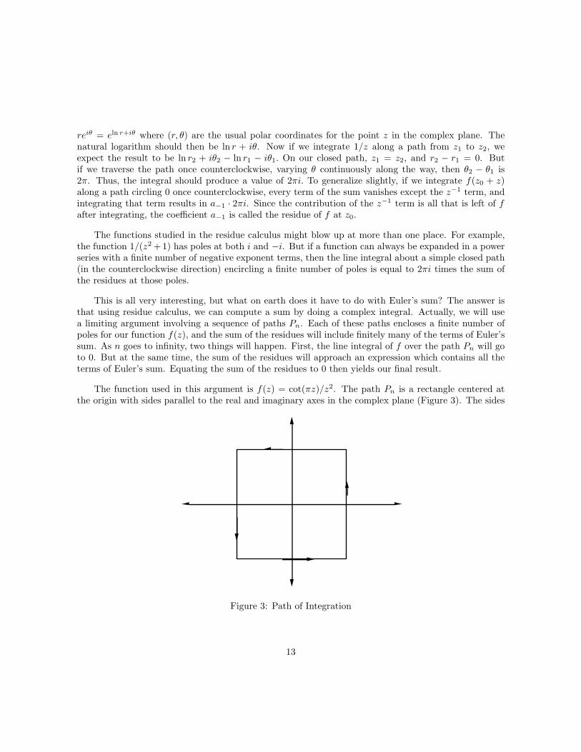
The function used in this argument is f(z) = cot(πz)/z2. The path Pn is a rectangle centered atthe origin with sides parallel to the real and imaginary axes in the complex plane (Figure 3). The sides

Figure 3: Path of Integration

13

intersect the real axis at ±(n+ 1/2) and the imaginary axis at ±ni. It may be shown that | cot(πz)| < 2for all z on the path Pn. (Actually, we can get a much more accurate bound than 2, but accuracy is notimportant here.) At the same time |z| ≥ n on the path, so |f(z)| < 2/n2. Bounding |f(z)| on the pathin this way permits us to estimate the integral. We have

|∮Pn

f(z)dz| < 2n2

(8n+ 2)

where 8n+ 2 is the length of the path. Now it is clear that as n goes to infinity, the integral goes to 0.

To complete the argument, we observe that f has poles at each of the integers, and determine thatthe residue is 1/πk2 at k 6= 0, and −π/3 at 0. Before carrying through these calculations, let us see howthe derivation of Euler’s formula concludes. Since the integral over Pn goes to 0, we infer that the 2πitimes the sum of all the residues is 0. Combining the residues at k and −k into a single term, this leadsto

−2π2i

3+ 4i

(1 +

122

+132

+142

+ · · ·)

= 0.

A trivial rearrangement of this equation reveals E = π2/6.

All that remains of this proof is the calculation of the residues. For the residue at 0, let us observethat

z cot(πz) = zcos(πz)sin(πz)

= z1− π2z2/2 + π4z4/24− · · ·πz − π3z3/6 + π5z5/120− · · ·

=1− π2z2/2 + π4z4/24− · · ·π − π3z2/6 + π5z4/120− · · · .

Using the long division algorithm, the ratio can be expressed as a power series. The first few terms areshown below.

z cot(πz) =1π− πz2

3− π3z4

45+ · · ·

By dividing both sides of this equation by z3, we derive

cot(πz)z2

=z−3

π− πz−1

3− π3z

45+ · · · .

Reading off the coefficient of z−1, we see that the residue at 0 is −π/3.

We use a slightly different method for the residue at k. Suppose that we calculated the power seriesfor f(k + z) as

f(k + z) = a−1z−1 + a0 + a1z + a2z

2 + · · · .Then

zf(k + z) = a−1 + a0z + a1z2 + a2z

3 + · · ·

14

and it is clear that

a−1 = limz→0

[zf(k + z)]

= limz→0

zcot(π(k + z))

(k + z)2

= limz→0

z

sin(π(k + z))cos(π(k + z))

(k + z)2.

Apply L’Hospital’s rule to the first factor, and find a−1 = 1/πk2. This gives the residue at k as previouslyasserted.

This calculation appears to rely on knowing in advance that the power series for f(k + z) has onlyone term with a negative power of z. Why were there no terms involving z−2, z−3, as there were forthe residue at 0? Actually, the answer is implicit in the limit we calculated above. Since zf(k + z) hasa limit at 0, its power series cannot have any terms with negative powers of z. Thus, every term of theseries for f(k+ z) must have an exponent of at least -1. Trying to apply the same argument at 0 wouldrequire evaluating the limit of zf(z) = cot(πz)/z. The failure of that step alerts us to the existence ofadditional negative exponent terms in the power series at 0.

It seems to me that the key insight in the foregoing proof is using an integral to evaluate a sum.In this case, it is the machinery of residue calculus that connects the sum and integral. Once f hasbeen defined, the remaining steps are a straightforward exercise of residue calculus methods. The nextargument also uses an integral to evaluate a sum, and again involves complex numbers, but it has adistinctly different flavor. There, we use vector algebra techniques in the context of Fourier analysis.

3.4 Fourier Analysis

Before discussing the proof using Fourier analysis, it will be helpful to review a little vector analysis. Inthree-dimensional space, think of a vector as a directed line segment (that is, a segment with an arrowat one end). For vectors a and b, a fundamental operation is the dot or inner product a · b. This maybe defined as the product of the lengths of a and b and the cosine of the angle between them. Thus, ifa and b are perpendicular, then a · b = 0, while for parallel a and b, the dot product is just the productof the lengths (or the negative of the product if the vectors are parallel and oppositely directed).

The inner product is useful in breaking down vectors into simple pieces. Let ex, ey, and ez bevectors of length 1 starting at the origin and pointing along the x, y, and z axes. Every other vector inspace can be built up using sums and multiples of these three special vectors. A typical example wouldbe something of the form 3ex + 5ey + 1.3ez. This is the vector which begins at the origin and ends atthe point (3,5,1.3). Just as the three coefficients, 3, 5, and 1.3, completely determine the vector in thisexample, so any vector is uniquely determined by its three coefficients relative to the e vectors.

Notice that since any two of the e vectors are perpendicular, their dot product is 0. And the dotproduct of any of these vectors with itself is 1. These two properties, which are characteristic of an

15

orthonormal basis, provide a simple way to compute the coefficients which describe any vector. Indeed,if we have a = (pex + qey + rez), then by taking the dot product of each side with ex we find p = a · ex.Similar reasoning leads to q = a ·ey and r = a ·ez. That is, the coefficient for each of the e vectors can befound by computing the dot product of a with that vector. As another consequence of orthonormality,observe that a · a = p2 + q2 + r2. The derivation of this identity,

a · a = (pex + qey + rez) · (pex + qey + rez)= p2ex · ex + q2ey · ey + r2ez · ez + 2pqex · ey + 2prex · ez + 2qrey · ez= p2 + q2 + r2

again uses the fact that the dot product of any of the e’s with itself is 1, while the dot product betweentwo different e’s is 0.

In Fourier analysis, there is a wonderful analogy with the ideas of vectors, dot products, and orthonor-mality. In place of vectors we deal with complex-valued functions of a real variable. The dot product oftwo functions is defined using integrals: f · g = (1/2π)

∫ π−π f(t)g(t)dt (the bar denotes complex conjuga-

tion). In place of the special vectors ex, ey, and ez, we have the functions 1 = e0it, e±it, e±2it, e±3it, · · · .These form an orthonormal basis, and any well behaved function f can be expressed using the basisfunctions in just the same way that vectors in space can be expressed in terms of the e vectors. Aswas the case for vectors, the coefficients for the basis functions are just dot products. Thus, if we writef(t) = · · ·+ a−2e

−2it + a−1e−it + a0 + a1e

it + a2e2it + · · · , then

a2 = f · e2it

=1

2π

∫ π

−πf(t)e−2itdt

and similarly for all the other coefficients. Finally, in Fourier analysis there is an analog for the formulaa · a = p2 + q2 + r2. Because the coefficients in the Fourier case can be complex numbers, it is theirsquared absolute values (not simply their squares) that must be summed, but otherwise the analogy isexact. Thus, we have the formula f · f = · · ·+ |a−2|2 + |a−1|2 + |a0|2 + |a1|2 + |a2|2 + · · ·. It is this lastfact that we use to derive the value of Euler’s sum.

Here is how it works. The function to use is f(t) = t. By direct calculation,

f · f =1

2π

∫ π

−πt2dt

=1

2πt3

3

π

−π

=π2

3.

Now we will compute f · f in terms of the coefficients ak. As an example, let’s calculate a2.

a2 =1

2π

∫ π

−πte−2itdt

16

=1

2π2it+ 1

4e−2it

π

−π

=i

2.

The last step in this calculation takes advantage of the fact that eπi = −1. A similar calculation donewith an arbitrary integer n in place of 2 discovers that an = ±i/n for all n except 0, and that a0 = 0.Thus, for every n but 0, |an| = 1/n, and · · · + |a−2|2 + |a−1|2 + |a0| + |a1|2 + |a2|2 + · · · is none otherthan Euler’s sum written twice. This leads to 2E = π2/3, and dividing by 2 completes the proof.

3.5 Interlude: An Application of Euler’s Result

Let’s take a break from all these proofs, and consider an application. If an infinite sum of positiveterms converges, it can be used to create a probability distribution. Just so for Euler’s sum. Letpk = (6/π2)(1/k2). Then the pk sum to 1, and can be regarded as a discrete probability distribution,with pk the probability of the kth outcome. Does this distribution actually have any use? As it turns out,it does. In fact, pk is the probability that two randomly selected positive integers have greatest commondivisor (GCD) equal to k. One must be a little careful about what is meant by randomly selecting aninteger, for there is obviously no way to make all the positive integers equally likely and still have totalprobability 1. This is a technical point that can be put aside for the moment, in favor of a heuristicapproach. To proceed, define qk to be the probability that two randomly selected positive integers haveGCD k. We show that qk = pk.

The GCD of integers a and b equals k if and only if two conditions hold. First, both integers mustbe multiples of k. Second, the GCD of a/k and b/k must be 1. Now the probability that two randomlyselected integers are both multiples of k is 1/k2. The probability that GCD(a/k, b/k) = 1, given thata and b are multiples of k, is just the same as the unconditional probability that two positive integershave GCD 1, for as a and b range over the multiples of k, a/k and b/k range over the full set of positiveintegers. Combining the two preceding observations shows that qk = q1(1/k2). Since the qk must sumto 1, we see that q1 = 6/π2, hence qk = pk, as asserted.

In retrospect, knowing the value of Euler’s sum was a necessary step in determining the distributionof the GCD function. As an interesting consequence, we can now assert that a randomly generatedfraction will be in lowest terms with probability 6/π2. I found these ideas in [1] (which comments onthe technical point we set aside above) and [13].

Let us return now to our tour of proofs and examine a final derivation.

17

3.6 A Real Integral with an Imaginary Value

The final proof was published by Russell [17]. It begins with the definite integral

I =∫ π/2

0

ln(2 cosx)dx.

Now 2 cosx = eix + e−ix = eix(1 + e−2ix). Therefore, ln(2 cosx) = ln(eix) + ln(1 + e−2ix) = ix+ ln(1 +e−2ix). We make the substitution in the integral and arrive at

I =∫ π/2

0

ix+ ln(1 + e−2ix)dx

= iπ2

8+∫ π/2

0

ln(1 + e−2ix)dx. (4)

The next step is to replace the logarithm with a power series, and integrate term by term. The powerseries expansion is [9, p.401]

ln(1 + x) = x− x2/2 + x3/3− x4/4 + · · ·

or, replacing x by e−2ix

ln(1 + e−2ix) = e−2ix − e−4ix/2 + e−6ix/3− e−8ix/4 + · · · .

Integrate: ∫ln(1 + e−2ix)dx =

e−2ix

−2i− e−4ix

−2i · 22+

e−6ix

−2i · 32− e−8ix

−2i · 42+ · · ·

=−12i

(e−2ix − e−4ix

22+e−6ix

32− e−8ix

42+ · · ·).

This last expression is to be evaluated from 0 to π/2. That yields∫ π/2

0

ln(1 + e−2ix)dx =−12i

(e−iπ − 1− e−2iπ − 122

+e−3iπ − 1

32− e−4iπ − 1

42+ · · ·).

Now every exponential either evaluates to 1 (for even multiples of iπ) or to -1 (for odd multiples).Therefore, half of the terms drop out, and the remaining terms are all fractions with a -2 in the numeratorand an odd square in the denominator. Thus∫ π/2

0

ln(1 + e−2ix)dx =1i(1 +

132

+152

+ · · ·).

As we have seen before, the odd terms of Euler’s sum add up to 3/4 of the total. Combining this withthe fact that 1/i = −i, we conclude that∫ π/2

0

ln(1 + e−2ix)dx =−3i

4E.

18

At this point, we must return to the integral we first considered. Substituting the expression justderived into (4), we obtain

I = i(π2

8− 3

4E).

But I is real, and it is equal to a pure imaginary. This forces both sides of the equation to vanish.Setting the right-hand side to 0 gives us the familiar conclusion E = π2/6. Setting the left-hand side to0 produces an added bonus: ∫ π/2

0

ln(cosx)dx = −π2

ln 2.

In this whirlwind of manipulations, there is probably nothing that would have disturbed Euler. Incontrast, a modern student of mathematics would find reasons for skepticism at practically every step.First off, the original integral is improper, so we need to worry about convergence. Next, in order to usethe natural logarithm for complex variables, we need to be sure that we can restrict the complex numbersto a suitable domain. (In this case, it is enough to observe that we never need to apply the logarithm toa negative real.) Thirdly, the power series for the natural logarithm converges within a circle of radius1 centered at 0 in the complex plane. Unfortunately, for every x in the domain of integration, e−2ix

is on the boundary of this circle, so that we must be concerned about convergence of the power series,too. (For this step we may appeal directly to a Theorem 3.44 of [16].) And finally, there is the term byterm integration of the sum. In general terms, we handle these problems by starting in the middle andworking our way out. The idea is to start with the series formulation of the integral, but let the upperlimit be less than π/2. Then we can justify the term by term integration and take a limit to reach theupper limit of π/2, determining the value for the integral in the process. Working in the other direction,now that we know that the integral exists in the case of the power series formulation, we are justifiedin performing the manipulations that generate the integral that the argument above started with. Thisverifies that the original improper integral is indeed defined. For additional comments on justifying thesteps in the proof, see [17].

4 ConclusionWe have seen a variety of proofs of Euler’s result. It is interesting how wide a range of mathematicalsubjects appeared in these proofs. Euler’s proof has the appearance of direct algebraic manipulation,but involves an unfounded assumption about the properties of power series. The first valid proof weconsidered works directly from the definition of convergent power series by providing bounds for partialsums of Euler’s series. Two proofs each involve replacing the sum with a different operation. Thus,in residue calculus, a sum of residues is replaced by a complex line integral, while in Fourier Analysis,a sum of squared coefficients is replaced by a dot product. And finally, two proofs use a technique ofinterchanging a sum and an integral to transform Euler’s series into another form that can be summeddirectly. It should come as no surprise that there are still more proofs of Euler’s formula (including afew by Euler himself). The interested reader is encouraged to consult the references for more approachesand additional references. Of historical interest is reference [11], the first edition of which appeared in1921. In this encyclopedic work, several proofs of Euler’s result can be found (see articles 136, 156, 189,

19

210) in the context of general procedures for manipulating and analyzing series expansions. The proofin article 210 is closely related to the fourier analysis proof given above.

Acknowledgments: Thanks are due Melvin Henriksen, Richard Katz, and Alan Krinik for alerting me to some of the

papers cited in the article, to Judith Grabiner and Mark McKinzie for help with the historical references, and to the

referees for many helpful suggestions.

References

[1] Aaron D. Abrams and Matteo J. Paris, The Probability that (a, b) = 1. College MathematicsJournal (23)1:47, January 1992.

[2] Tom M. Apostol, Another Elementary Proof of Euler’s Formula for ζ(2n). American MathematicalMonthly, 80(4):425 – 431, April 1973.

[3] Tom M. Apostol, A Proof that Euler Missed: Evaluating ζ(2) the Easy Way. MathematicalIntelligencer, 5(3):59 – 60, Summer 1983.

[4] Raymond Ayoub, Euler and the Zeta Function. American Mathematical Monthly, 81(10):1067 –1085, December 1974.

[5] Paul Erdos and Underwood Dudley, Some Remarks and Problems in Number Theory Related tothe Work of Euler. Mathematics Magazine, 56(5):292 – 298, November 1983.

[6] Leonhard Euler, De Summis Serierum Reciprocarum. Comm. acad. sci. Petrop., 7 (1734/35), 1740,pp. 123 – 134 = Opera Omnia, 14, 73 – 86.

[7] Daniel P. Giesy, Still Another Elementary Proof that∑

1/k2 = π2/6. Mathematics Magazine,45(3):148 – 149, March 1972.

[8] Judith V. Grabiner, Who Gave You the Epsilon? Cauchy and the Origins of Rigorous Calculus.American Mathematical Monthly, 90(3):185 – 194, March 1983.

[9] Melvin Henriksen and Milton Lees, Single Variable Calculus (New York: Worth, 1970).

[10] Morris Kline, Euler and Infinite Series. Mathematics Magazine, 56(5):307 – 314, November 1983.

[11] Konrad Knopp, Theory and Application of Infinite Series (Translated from the second Germanedition and revised in accordance with the fourth) (New York: Hafner, ca. 1947).

[12] W. A. J. Luxemburg, What is nonstandard analysis? American Mathematical Monthly (80)6 partII:38–67, June-July 1973.

[13] Bill Leonard and Harris S. Shultz, A Computer Verification of a Pretty Mathematical Result.Mathematical Gazette (72)459:7–10, March 1988.

[14] Mark B. McKinzie and Curtis D. Tuckey, Euler’s Proof of∑∞n=1 1/n2 = π2/6. Annual Meeting of

the American Mathematics Society, San Antonio, Texas, January 1993.

[15] Ioannis Papadimitriou, A Simple Proof of the Formula∑∞k=1 k

−2 = π2/6. American MathematicalMonthly, 80(4):424 – 425, April 1973.

20

[16] Walter Rudin, Principles of Mathematical Analysis, 2nd Edition (New York: McGraw-Hill, 1964).

[17] Dennis C. Russell, Another Eulerian-Type Proof. Mathematics Magazine, 60(5): 349, December1991.

[18] Nicholas Shea, Summing the Series 112 + 1

22 + 132 + · · ·. Mathematical Spectrum, 21(2):49 – 55,

1988-89.

[19] Alfred Van der Poorten, A Proof that Euler Missed . . .Apery’s Proof of the Irrationality of ζ(3).Mathematical Intelligencer, 1(4):195 – 203, 1978-79.

[20] Don Bernard Zagier, Zeta Functions in Number Theory. Annual Meeting of the American Mathe-matics Society, Phoenix, Arizona, January 1989.

21