skewness in stock returns: reconciling the evidence …ruialbuquerque.webs.com/rev. financ....
TRANSCRIPT
Skewness in Stock Returns:Reconciling the Evidence on Firm VersusAggregate Returns
Rui AlbuquerqueBoston University, Catolica-Lisbon School of Business and Economics
Aggregate stock market returns display negative skewness. Firm stock returns displaypositive skewness. The large literature that tries to explain the first stylized fact ignoresthe second. This article provides a unified theory that reconciles the two facts byexplicitly modeling firm-level heterogeneity. I build a stationary asset pricing model of firmannouncement events where firm returns display positive skewness. I then show that cross-sectional heterogeneity in firm announcement events can lead to conditional asymmetricstock return correlations and negative skewness in aggregate returns. I provide evidenceconsistent with the model predictions. (JEL G12, G14, D82)
Aggregate stock market returns display negative skewness, the propensityto generate negative returns with greater probability than suggested by asymmetric distribution. A large body of literature has aimed to explain thisstylized fact about the distribution of aggregate stock returns (e.g.,Fama1965; Black 1976; Christie 1982; Blanchard and Watson 1982;Pindyck1984; French, Schwert, and Stambaugh 1987; Hong and Stein 2003). Theevidence on aggregate returns contrasts with another stylized fact; namely,that firm-level returns are positively skewed. For this reason, theories ofnegative skewness that model single-firm stock markets necessarily depict anincomplete picture. In this article, I provide a unified theory for both stylizedfacts by explicitly modeling firm-level heterogeneity and studying the effectsof aggregation, and present evidence consistent with the theory.
The implications from the disconnect between firm-level return skewnessand aggregate return skewness are best illustrated using the definition of
I would like to thank Pietro Veronesi (the Editor) and two anonymous referees for constructive suggestions,and also the comments from Adlai Fisher, Marcin Kacperczyk, Emilio Osambela, Lukasz Pomorski, ClaraRaposo, Martin Schneider, Kevin Sheppard, and Grigory Vilkov as well as from seminar participants at BostonUniversity, Catolica-Lisbon, ESSEC, Michigan Ross School of Business, Said School of Business and Oxford-Man Institute of Oxford University, University of Miami, and at the 2010 European Finance Association andthe 2011 UBC Winter Finance conferences. Financial support from a grant from the Portuguese Foundation forScience and Technology-FCT is gratefully acknowledged. Send correspondence to: Rui Albuquerque, FinanceDepartment, Boston University School of Management, 595 Commonwealth Avenue, Boston, MA 02215.E-mail: [email protected]. The author is also affiliated with the Centre for Economic Policy Research and theEuropean Corporate Governance Institute. The usual disclaimer applies.
c© The Author 2012. Published by Oxford University Press on behalf of The Society for Financial Studies.All rights reserved. For Permissions, please e-mail: [email protected]:10.1093/rfs/hhr144
RFS Advance Access published January 9, 2012 at B
iblioteca Joao Paulo II - Universidade C
at?lica Portuguesa on January 12, 2012http://rfs.oxfordjournals.org/
Dow
nloaded from

TheReview of Financial Studies / v 00 n 0 2012
sampleskewness of a portfolio return. Skewness of a portfolio return is the sumof mean firm-return skewness andcoskewnessterms. Because mean firm skew-ness is positive, negative portfolio-return skewness must be caused by negativecoskewness terms. The coskewness terms capture the average comovement inone firm’s return with the variance of the portfolio that comprises the remainingfirms. Thus, coskewness depends on the cross-sectional heterogeneity offirm comovement, which makes the observed negative skewness in aggregatereturns a cross-sectional phenomenon.
This article argues that the behavior of stock prices around certain firmannouncement events is consistent with the existence of positive skewness infirm returns and that cross-sectional heterogeneity in the timing of these eventscan account for the negative skewness in aggregate returns.
The article provides a stationary asset pricing model of cash payout andearnings announcement events that captures the basic stylized facts on volatil-ity and mean returns around such events. When cash payouts are periodic, cashflow news is discounted according to the time remaining until the next payout,and the impact of cash flow news on the conditional return volatility is greaterfor news released closer to the payout. The model predicts that conditionalvolatility exhibits a spike around the payout event despite homoscedastic cash-flow news shocks. The presence of a risk-return trade-off in the model impliesthat this property applies also to conditional mean returns, and the rarity ofspikes induces positive skewness in conditional mean returns. Similarly, themodel predicts conditionally higher return volatility and mean returns aroundearnings announcement events due to large contemporaneous informationflows. Firm returns may thus display sporadic and short-lived periods of highvolatility and high mean returns around earnings announcements, and positiveskewness in conditional mean returns.
The simplicity of the model allows for a complete characterization ofthe conditional and unconditional distributional properties of equilibriumreturns. I show that the unconditional distribution of equilibrium returns isa mixture of normals distribution. Under a mixture of normals distribution,skewness in stock returns is given by two components. The first componentis skewness in conditional mean returns. The second component captures theassociation between expected returns and conditional return variance and ispositive given the risk-return trade-off embedded in the model. With bothterms positive, the model can generate positive skewness in firm-level stockreturns.
To study market return skewness, I introduce heterogeneity in firms’announcement events. When firms have different announcement event dates,the high mean return and return volatility of some firms around their eventdate contrasts with the low return volatility of the portfolio of the remainingfirms and may generate negative coskewness in the market portfolio. Inthe model, sharp stock market downturns are likely to occur during anannouncement season in which a significant fraction of firms display high
2
at Biblioteca Joao Paulo II - U
niversidade Cat?lica Portuguesa on January 12, 2012
http://rfs.oxfordjournals.org/D
ownloaded from

Skewness in Stock Returns: Reconciling the Evidence on Firm versus Aggregate Returns
return volatility and strong comovement with the market, while the restdisplay low expected returns and low return volatility. These periods generateconditional asymmetry in stock correlations: stocks become more stronglycorrelated with the market return in a market downturn than in a marketupturn.
The article provides evidence consistent with the above model predictions.Using Centre for Research in Security Prices (CRSP) daily stock returns tocompute skewness over six-month periods from 1973 to 2009, I documenttwo stylized facts. First, firm-level skewness is higher than aggregate skewness96% of the time. Second, firm-level return skewness is always positive (exceptin the second half of 1987), whereas market skewness is almost alwaysnegative.
The evidence that the cross-sectional dispersion in event dates can producethe correct sign for aggregate return coskewness uses data on earningsannouncement events. As in the model, earnings announcements are associatedwith brief periods of high volatility and high mean returns (e.g.,Beaver 1968;Ball and Kothari 1991; Cohen et al. 2007). I use earnings announcement datesover the 1973 to 2009 period from the merged CRSP/Compustat quarterlyfile. I construct two experiments, both of which use daily return data oversix-month periods. In the first experiment, I form portfolios of firms basedon the calendar week of their first earnings announcement in each semester. Ithen group the firms in the first portfolio (first-week announcers) with thosefirms announcingk weeks later and report the six-month portfolio returnskewness. I show that, as in the model, there is a symmetric U-shaped patternin skewness: the portfolio of firms that announce in weeks 1 and 2 hassimilar return skewness to the portfolio of firms that announce in weeks 13and 1, and their skewness is higher than the skewness in any other portfolioconfiguration.
In the second experiment, I form portfolios of firms that announce in weeks1 throughk in the quarter fork = 2, . . . ,13, and report the respective portfolioreturn skewness. This experiment constructs stock markets with announcementseasons. I show that, consistent with the model, there is a negative relationshipbetween skewness and the increased heterogeneity that results from addingdispersion in event dates. I also show that portfolio skewness in the model canbe negative if sufficient heterogeneity in event dates is allowed.
The predictive power of the model hinges on information flowing tothe market in the form of announcement seasons. Consistent with otherstudies (e.g.,Chambers and Penman 1984; Kross and Schroeder 1984),I show that firms in the United States tend to announce between weekstwo and eight in each quarter, giving rise to an earnings announcementseason. The beginning of an announcement season is also the period inthe model that most contributes to the overall negative skewness in themarket. Consistent with this model prediction, I split aggregate skewnessinto its weekly components and document that aggregate skewness is
3
at Biblioteca Joao Paulo II - U
niversidade Cat?lica Portuguesa on January 12, 2012
http://rfs.oxfordjournals.org/D
ownloaded from

TheReview of Financial Studies / v 00 n 0 2012
particularly negative around the beginning of an earnings announcementseason.
An alternative explanation for why market skewness differs in sign fromfirm skewness is the existence of a negatively skewed return factor (seeDuffee 1995). FollowingDuffee (1995), I remove the market return—anegatively skewed factor—from firm returns to obtain “idiosyncratic” returns.I show that while some results are weaker when CAPM-based idiosyncraticreturns are used, the evidence is still broadly consistent with the model.Ideally, the use of structural models that nest various theories of negativeaggregate skewness can provide for more statistically powerful identificationstrategies.
The model is related to the literature that analyzes the flow of informationin the stock market (e.g.,He and Wang 1995) and the literature that studiesproperties of stock returns around public news events (e.g.,Kim and Verrecchia1991, 1994). Especially relevant is the work ofAcharya, DeMarzo, andKremer (forthcoming). They study the optimal release of information andthe clustering of announcements upon public news releases. In their model,as in Dye (1990), firms delay the release of bad news, which gives rise topositively skewed firm values. In addition, they show that when firms canpreempt the release of public industry news, there is clustering of bad newsupon the announcement, which, they argue, could give rise to conditionalnegative aggregate skewness. There are two main differences between theirsetting and mine. First, the mechanism in my article does not rely on theendogeneity of the decision to release information. Acharya et al. have amodel of voluntary disclosures, which are rare and difficult to predict (seeBhojraj, Li, and Yang 2010). In this article, I model and present evidencebased on earnings announcements, which are mandatory and generally morepredictable (e.g.,Givoly and Palmon 1982;Chambers and Penman 1984).Second, Acharya et al. present a result about conditional skewness, whereasmy result and the data presented speak to unconditional skewness in marketreturns.
Many studies have focused on asymmetric volatility as an explanationfor negative skewness in aggregate stock returns.Black (1976) andChristie(1982) posit the existence of a leverage effect, whereby a low price leadsto increased market leverage, which in turn leads to high volatility (see alsoVeronesi 1999). Pindyck (1984), French, Schwert, and Stambaugh(1987),Campbell and Hentschel(1992), Bekaert and Wu(2000), Wu (2001), andVeronesi(2004) further propose the existence of a volatility feedback effect,whereby high volatility is associated with a high risk premium and a lowprice. Blanchard and Watson(1982) show that negative skewness can resultfrom the bursting of stock price bubbles.Hong and Stein(2003) hypothesizethat short-sales constraints limit the market’s ability to incorporate bad news.According to their model, when more bad news arrives in the market, the priceresponds to the cumulative effect of news and falls at a time when volatility
4
at Biblioteca Joao Paulo II - U
niversidade Cat?lica Portuguesa on January 12, 2012
http://rfs.oxfordjournals.org/D
ownloaded from
Skewness in Stock Returns: Reconciling the Evidence on Firm versus Aggregate Returns
may be high (however, seeBris, Goetzmann, and Zhu 2007).1 Thesearticleshave made important contributions to our understanding of the dynamics ofreturn volatility and skewness, but they do not address the disconnect betweenfirm skewness and market skewness. The current article contributes to thisliterature by providing a bottom-up theory for negative skewness in aggregatestock returns that explicitly models positive skewness in firm-level returnsand firm-level heterogeneity. This article also contributes to the literatureby documenting empirically the sources of negative skewness in aggregatereturns: asymmetric correlations between firm and market returns explain thenegative skewness in market returns in this article. This prediction is consistentwith the conditional asymmetry in stock correlations found inLongin andSolnik (2001) andAng and Chen(2002), where market downturns are shownto be associated with higher stock correlations.
The model in this article is consistent with the evidence from dividend andearnings announcements.Aharony and Swary(1980),Kalay and Loewenstein(1985), andAmihud and Li (2006) show that dividend announcements areassociated with high returns and high volatility of stock returns.Beaver(1968),Givoly and Palmon(1982),Ball and Kothari(1991),Cohen et al.(2007), andothers show that the high expected returns around earnings announcementsare also associated with high volatility.Patton and Verardo(2010) documentan economically and statistically significant increase in firm beta on days ofearnings announcements. Finally, there is evidence that firm-level stock returnsare well described by a mixture of normals distribution (seeKon 1984;Zangari1996;Haas, Mittnik, and Paolella 2004).
The article is organized as follows. Section1 presents several facts aboutskewness and discusses the need to model cross-sectional heterogeneity.Section2 describes the basic model and presents the stock market equilib-rium. Section3 extends the model to incomplete information and earningsannouncement events. Section4 analyzes the skewness properties of aggregatestock returns. Section5 presents evidence on the article’s main hypotheses, andSection6 concludes. The Appendix contains the proofs of the propositions andresults on the correlated cash flow model.
1. Some Skewness Facts
This section starts by documenting several well-known facts about firm-leveland aggregate return skewness. Figure1 plots the time series of the mean firmstock return skewness and of skewness in the equally weighted market returncomputed using six months of daily data. The return is the holding periodarithmetic return from CRSP, inclusive of dividends. The data are further
1 For models of positive skewness at the firm level, see Acharya et al. (forthcoming),Dye (1990),Duffee(2002),Grullon, Lyandres, and Zhdanov(forthcoming),Hong, Wang, and Yu(2008), andXu (2007).Hong, Stein, andYu (2007) develop a model that predicts negatively skewed returns for glamour stocks and positively skewedreturns for value stocks.
5
at Biblioteca Joao Paulo II - U
niversidade Cat?lica Portuguesa on January 12, 2012
http://rfs.oxfordjournals.org/D
ownloaded from

The Review of Financial Studies / v 00 n 0 2012
Figure 1Skewness in firm-level and aggregate stock returnsThe figure plots mean skewness in daily firm-level returns (dashed line) and skewness in the equally weightedmarket return (solid line), both computed using six months of trading data. Data comprise all firms in CRSPwith complete daily return data by semester. Period of analysis is January 1, 1973, to December 31, 2009.
described in Section5below. Four salient stylized facts emerge from the figure.First, firm-level skewness is always positive, except in the second half of 1987.Second, skewness in market returns is almost always negative, representing77% of the observations. Third, and as a combination of the two factsabove, most semesters of large negative skewness in market returns are notaccompanied by negative skewness in firm-level returns. Fourth, firm skewnessis higher than aggregate skewness in 96% of the semesters. Because skewnessis generally lower and more often negative for larger firms, I reproduce thesame statistics using value-weighted mean (or median) firm skewness andvalue-weighted market return skewness. Not surprisingly, the value-weightedmean (or median) of firm skewness is lower, but the general gist of the resultsabove is unaffected. Results are also robust to using logarithmic returns andare available upon request.
To better understand these results and the need for cross-sectional hetero-geneity in a model-free way, it is useful to write the expression for samplenonstandardized skewness for a market composed ofN firms (i.e., the sampleestimate of the third-centered moment of returns). Assuming equal weightsfor simplicity, let r pt = N−1∑N
i =1 ri t be the timet market return,r i =T−1∑T
t=1 ri t be the mean sample return for firmi , andr p = T−1∑Tt=1 r pt be
6
at Biblioteca Joao Paulo II - U
niversidade Cat?lica Portuguesa on January 12, 2012
http://rfs.oxfordjournals.org/D
ownloaded from
Skewness in Stock Returns: Reconciling the Evidence on Firm versus Aggregate Returns
themean sample market return. Then, sample nonstandardized skewness is
T−1∑
t
(r pt − r p
)3 =1
N3
N∑
i =1
1
T
∑
t
(ri t − r i )3 (1)
+3
T N3
∑
t
N∑
i =1
(ri t − r i )
N∑
i ′ 6=i
(ri ′t − r i ′)2
+6
T N3
∑
t
N∑
i =1
(ri t − r i )
N∑
i ′>i
N∑
l>i ′(ri ′t − r i ′) (rl t − r l ) .
Thefirst term in (1) is the mean of firm skewness and, as Figure1 shows, it ispositive. The second and third terms in (1) are the coskewness terms. I labelthese termsco-vol andco-cov, respectively. Together, they must be negativefor skewness in market returns to be negative.
Loosely speaking, the coskewness terms capture the average comovement inone firm’s return with the variance of the portfolio that comprises the remainingfirms. Thus, coskewness depends on the cross-sectional heterogeneity of firmcomovement, implying that the negative skewness in aggregate returns isa cross-sectional phenomenon. Specifically, theco-vol term describes howone firm’s return comoves with the return variance in the other firms in theportfolio. Theco-covterm describes how one firm’s return behaves at times ofgreater or smaller comovement in other stocks.
Next, I show that theco-cov term dominates the sum in (1). Thenumber of firms in a portfolio does not directly affect the calculation ofsample skewness. Inspection of Equation (1) reveals thatN−3 multipliesevery term. At the same time,N−3 also multiplies every term in the de-nominator of standardized skewness, because standardized skewness equalsT−1∑
t
(r pt − r p
)3/[T−1∑
t
(r pt − r p
)2]3/2, canceling off in the calculationof skewness. Where the number of firms matters is in the weights placed in thevarious terms. Observe that there areN firm-level skewness terms,N (N − 1)terms inco-vol, andN!/ [3! (N − 3)!] terms inco-cov. Hence, as the numberof firms increases, the number of terms associated withco-covincreases fasterthan the number of terms associated with any other component of skewness.This does not immediately imply that theco-cov terms dominate the sum,because it may be the case that their component terms cancel each other out.In Figure 2, I plot the ratio of the standardizedco-cov term to the sampleskewness of market returns. With a ratio close to 100%, on average, the figuresuggests that it is theco-covterm that drives negative skewness at the marketlevel.
What determines the sign of theco-covterm is the presence of conditionalasymmetries in stock correlations. Take a market downturn characterizedby the average firm experiencing a return below the mean. If the pairwise
7
at Biblioteca Joao Paulo II - U
niversidade Cat?lica Portuguesa on January 12, 2012
http://rfs.oxfordjournals.org/D
ownloaded from
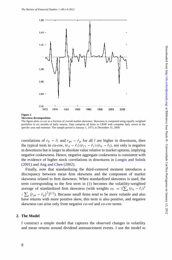
The Review of Financial Studies / v 00 n 0 2012
Figure 2Skewness decompositionThe figure plotsco-covas a fraction of overall market skewness. Skewness is computed using equally weightedportfolios in six months of daily returns. Data comprise all firms in CRSP with complete daily return in thespecific year and semester. The sample period is January 1, 1973, to December 31, 2009.
correlations ofrlt − r l and r pt − r p for all l are higher in downturns, thenthe typical term inco-cov, (ri t − r i ) (ri ′t − r i ′) (rlt − r l ), not only is negativein downturns but is larger in absolute value relative to market upturns, implyingnegative coskewness. Hence, negative aggregate coskewness is consistent withthe evidence of higher stock correlations in downturns inLongin and Solnik(2001) andAng and Chen(2002).
Finally, note that standardizing the third-centered moment introduces adiscrepancy between mean firm skewness and the component of marketskewness related to firm skewness. When standardized skewness is used, theterm corresponding to the first term in (1) becomes the volatility-weightedaverage of standardized firm skewness (with weightsωi = [
∑t (ri t − r i )
2
/∑
t
(r pt − r p
)2]3/2). Because small firms tend to be more volatile and alsohave returns with more positive skew, this term is also positive, and negativeskewness can arise only from negativeco-volandco-covterms.
2. The Model
I construct a simple model that captures the observed changes in volatilityand mean returns around dividend announcement events. I use the model to
8
at Biblioteca Joao Paulo II - U
niversidade Cat?lica Portuguesa on January 12, 2012
http://rfs.oxfordjournals.org/D
ownloaded from

Skewness in Stock Returns: Reconciling the Evidence on Firm versus Aggregate Returns
show that these patterns in the conditional mean and volatility of returns leadto positive skewness in firm-level returns. In Section3, I study a model ofincomplete information with earnings announcement events that shares similarproperties of returns.
2.1 Investment opportunitiesTime is discrete and indexed byt = 1,2, . . .. There is a risk-free asset withperfectly elastic supply that earns the gross rate of return ofR > 1. Fornow, consider a stock market with one stock only that has a fixed supply ofone share. The general case is treated in Section4. The share of the stock isinfinitely divisible and trades competitively at timet at the ex dividend pricePt . A dividend is announced (and simultaneously paid) everyK + 1 periods,
Dt = Ft +K∑
j =0
εDt−K+ j . (2)
If t correspondsto a nondividend period, thenDt = 0.To keep track of the time to the next dividend announcement, trading periods
are further identified by event time using the indexk = 0, . . . , K , wherek = 0refers to a dividend-paying period, andk > 0 refers to a non-dividend-payingperiod. It helps to think of a trading period as one week and ofK +1 periods asone quarter: weekk in the quarter isk weeks since the last dividend payment,andK + 1 − k weeks to the next dividend payment.
The dividend can be decomposed into a persistent component,
Ft = ρF Ft−1 + εFt , 0 ≤ ρF ≤ 1,
with εFt ∼ N
(0,σ 2
F
), and a transitory component,
∑Kj =0 εD
t−K+ j , with
εDt ∼ N
(0,σ 2
D
). Note that dividend shocks are conditionally homoscedastic,
and thus any conditional heteroscedasticity in equilibrium returns is generatedendogenously.
Denote byPkt and Qk
t the stock price and return, respectively, that occurin period t , k periods after the last dividend payout. The excess return in adividend-paying period is
Q0t ≡ P0
t + Dt − RPKt−1,
andin a non-dividend-paying period is
Qkt ≡ Pk
t − RPk−1t−1 .
2.2 Investors’ problemThere is a continuum of identical investors with unit mass. Investors choosetheir timet asset allocation,θt , to maximize expected utility over next-period
9
at Biblioteca Joao Paulo II - U
niversidade Cat?lica Portuguesa on January 12, 2012
http://rfs.oxfordjournals.org/D
ownloaded from

TheReview of Financial Studies / v 00 n 0 2012
wealth,Wt+1,
E[− exp−γ Wt+1 |It
], (3)
whereγ > 0 is the coefficient of absolute risk aversion. The maximization issubject to the budget constraint,
Wt+1 = Qk+1t+1θt + RWt , (4)
andthe information set,
It ={
Pt−s, Dt−s, Ft−s, εDt−s
}
s≥0. (5)
For simplicity, I adopt the shorthand notation for the expectations operator,Et [.] = E [.|It ].
2.3 Stock market equilibriumInvestors trade competitively in the stock market, making their asset allocationwhile taking prices as given. In equilibrium, the stock price is consistent withmarket clearing:
θt = 1. (6)
In the Appendix, I show that
Proposition 1. The equilibrium price function is
Pkt = pk + Γk Ft + R−(K+1−k)
k−1∑
j =0
εDt− j , (7)
for Γk ≡ (ρF/R)K+1−k
1−(ρF /R)K+1 andanyk = 0, . . . , K . The constantspk < 0 are given
by
pk = −1
RK+1 − 1
K∑
j =0
RK− j Et
[Qk+1+ j
t+1
], (8)
wherefor anyk, Et
[Qk+1+K
t+1
]= Et
[Qk
t+1
].
The expression in Equation (7) uses the convention that∑−1
j =0 εDt− j = 0.
The stock price atk reflects the present value of dividends conditional onall available information. The present value accounts for the fact that attime t—afterk periods have elapsed since the last dividend payment—it willtake anotherK + 1 − k periods until dividends are paid again. Consider
10
at Biblioteca Joao Paulo II - U
niversidade Cat?lica Portuguesa on January 12, 2012
http://rfs.oxfordjournals.org/D
ownloaded from

Skewness in Stock Returns: Reconciling the Evidence on Firm versus Aggregate Returns
first the coefficient associated withFt . With k = 0, the coefficient is[(R/ρF )K+1 − 1
]−1, and the stock resembles a perpetuity discounted at rate
(R/ρF )K+1−1.This is because the next payment arises inK +1 periods and isdiscounted byRK+1, and by that timeFt will have decreased in expectation byρK+1
F . K + 1 periods later, another payment occurs, which is also discountedat the same rate, and so on.
The transitory shockεD entersthe stock price function because investorslearn about it before it is paid as a dividend:εD
t entersthe price function attime t with a coefficient ofR−(K−k), whereasεD
t+1 entersthe price functionat time t + 1 with a coefficient ofR−(K−k−1) > R−(K−k). Despite beingtransitory,εD
t hasde facto persistence of one until the next dividend payment,and persistence of zero thereafter.
2.4 Conditional distribution of stock returnsDefine the conditional mean return asμk = Et
[Qk+1
t+1
]andthe conditional
volatility of returns asσ 2k = Et
[Qk+1
t+1 − Et
(Qk+1
t+1
)]2. The investors’ first-
order condition together with the stock market clearing condition requires that
μk = γ σ 2k . (9)
To solve for the equilibrium values of{μk, σ
2k
}k, use the price function
above to express excess returns as
Qkt = pk − Rpk−1 + Γkε
Ft + R−(K+1−k)εD
t , (10)
for anyk. In this expression,Q0t is recovered by replacingk with K + 1 and
noting thatpK+1 = p0 andQK+1t = Q0
t . Therefore,
Corollary 1. The conditional distribution of stock returns is normal,
Qk+1t+1 |t ∼ N
(μk, σ
2k
),
with μk given by Equation (9) andσ 2k given by
σ 2k = Γ2
kσ2F + R−2(K+1−k)σ 2
D. (11)
Theconditional mean and volatility of the stock return increase monotonicallyand are convex ink, all else equal.
The corollary states that the conditional stock return volatility increaseswith k despite the fact that the cash flow shocksεF
t andεDt areconditionally
homoscedastic. The intuition is that cash flow news that occurs further awayfrom the dividend payment is more highly discounted and contributes lessto risk than cash flow news that occurs closer to the dividend payment.
11
at Biblioteca Joao Paulo II - U
niversidade Cat?lica Portuguesa on January 12, 2012
http://rfs.oxfordjournals.org/D
ownloaded from

TheReview of Financial Studies / v 00 n 0 2012
Further, discounting penalizes news asymmetrically (i.e., conditional meanand volatility of stock returns are convex ink), which yields distributions ofconditional meanreturns andconditional volatilityof returns that are positivelyskewed.
Quantitatively, the effect of discounting on conditional heteroscedasticityvia the persistent shocks can be very large even for small interest rates.Consider the impact ofk on the coefficient associated withσ 2
F in Equation(11). Specifically, evaluate the difference in coefficients atk = 0 andk = Kand take the limit asρF/R → 1. Applying L’Hopital’s rule,
limρF /R→1
(ρF/R)2 (1 − (ρF/R)2K )
(1 − (ρF/R)K+1)2
= +∞.
Intuitively, a lower interest rate (and higher persistenceρF ) reduces the impactof discounting associated with cash flow news that is released before the nextpayout, but increases the value of the perpetuity associated with the news. Thesecond effect is stronger than the first producing the result. Because transitoryshocks lack the second effect, whenR → 1 the discounting effect throughtransitory shocks disappears.
The result in the corollary shows that the model is consistent with theevidence that dividend announcements are associated with both higher meanreturns and higher volatility (e.g.,Aharony and Swary 1980; Kalay andLoewenstein 1985). More recently,Amihud and Li(2006) show evidence of adeclining, but still significant, dividend announcement effect.
2.5 Unconditional distribution of stock returnsCorollary 1 shows that the firm’s stock return is conditionally normallydistributed with meanμk and varianceσ 2
k . The unconditional distributionof the firm’s stock return is not normal because the mean and variance ofa randomly drawn return observation depend onk. In fact, because ak-period stock return is drawn from a normal densityφ
(Q; μk, σ
2k
)andsuch
observations occur with frequency 1/(K + 1), the unconditional distributionof returns is a mixture of normals distribution. Formally,
Proposition 2. For K ≥ 1, the unconditional distribution of stock returns isa mixture of normals distribution with density
f (Q) =1
K + 1
K∑
k=0
φ(
Q; μk, σ2k
), (12)
whereφ (.) is the normal density function. ForK = 0, returns are uncondi-tionally normally distributed.
12
at Biblioteca Joao Paulo II - U
niversidade Cat?lica Portuguesa on January 12, 2012
http://rfs.oxfordjournals.org/D
ownloaded from

Skewness in Stock Returns: Reconciling the Evidence on Firm versus Aggregate Returns
The periodicity of dividends—by generating time-varying conditionalvolatility in stock returns—leads to the derived mixture of normals distributionfor stock returns forK ≥ 1. This result provides a theoretical justification forattempting to fit a mixture of normals distribution to stock returns (e.g.,Fama1965;Granger and Orr 1972;Kon 1984;Tucker 1992).
In the Appendix, I prove the following corollary:
Corollary 2. The unconditional mean and variance of stock returns are
E (Qt+1) =1
K + 1
K∑
k=0
μk,
Var (Qt+1) =1
K + 1
K∑
k=0
[σ 2
k + (μk − E (Qt+1))2].
Theunconditional (nonstandardized) skewness in stock returns is
E[(Q − E (Qt+1))
3]
=1
K + 1
K∑
k=0
(μk − E (Qt+1))3
+3
(K + 1)2
K∑
k=0
∑
j <k
(σ 2
k − σ 2j
) (μk − μ j
). (13)
The unconditional mean return is simply the mean of thek-conditional expected returns. The unconditional mean variance is themean of thek-conditional variances plus the variance of thek-conditionalmeans.
Skewness in stock returns can be decomposed into two terms. The first termin (13) is the level of skewness in expected returns,μk. For K ≤ 3, it ispossible to show that this term is non-negative because of the monotonicityand convexity ofμk.2 For larger values ofK , it is not possible to sign thisterm, but numerically it is always found to be positive. Intuitively, this term ispositive because an increasing and convexμk in event time produces a spike-like pattern in expected returns in event time. The second term describes theimpact on skewness of the comovement between return volatility and expectedreturns. The risk-return trade-off implied by Equation (9) guarantees that thesecond term in (13) is positive: periods of high expected returns are associatedwith periods of high volatility. In summary, stock returns display positiveskewness.
2 Theproof is quite lengthy and is omitted but is available upon request.
13
at Biblioteca Joao Paulo II - U
niversidade Cat?lica Portuguesa on January 12, 2012
http://rfs.oxfordjournals.org/D
ownloaded from

TheReview of Financial Studies / v 00 n 0 2012
2.6 DiscussionThe stochastic discount factor implicit in the single firm equilibrium formu-lated above is3
mk+1t+1 = γ exp
[−γμk+1 − γ Γk+1ε
Ft+1 − γ R−(K+1−k)εD
t+1
].
It can be derived directly from the first-order conditions if written as
Et
[mk+1
t+1 Qk+1t+1
]= 0, and imposing the market clearing condition,θt = 1.
Thestochastic discount factor changes with both calendar time as well as eventtime, reflecting the fact that shocks to dividends carry a higher risk premiumthe closer they are to a payout period. Formulating the problem as partialequilibrium and assuming an exogenous stochastic discount factor, as opposedto specifying preferences and budget constraints, is less restrictive and offers asimple and general approach to modeling the effects described in this article,but lacks microfoundations. This article provides a microfoundation for event-time variation in the stochastic discount factor.
The model generates skewness in firm-level stock returns by making use ofthe time-series patterns in volatility that arise from having cash payouts spreadout over time. While these patterns in conditional volatility are consistent withthe evidence, there could be other explanations for the same facts. For example,it could be the case that the resolution of uncertainty afforded by earningsannouncements also results in greater volatility and higher expected returns.I explore this idea in the next section by modeling earnings announcements.
The model takes the cash payout dates as fully predictable, which eliminatesconsiderations about strategic timing of events and timing-related risk. Whilethis assumption is made for tractability, it finds some support in the data(Kalay and Loewenstein 1985). Likewise, earnings announcement days—to be discussed next—are generally predictable (e.g.,Givoly and Palmon1982; Chambers and Penman 1984; Kross and Schroeder 1984), and thispredictability arises mostly from past earnings announcement behavior, whichhas been attributed to tradition (e.g.,Givoly and Palmon 1982).
Positive skewness arises despite the fact that prices and returns are con-ditionally normally distributed. The source of skewness in the model isthus distinct from that which affects arithmetic returns mechanically due totruncation at zero. This benefit, due to exponential utility and normal shocks,comes at the cost of having negative prices with positive probability. Tominimize this probability, it is customary to add a positive long-run meandividend to the process in Equation (2). Because all main results (i.e., patternsin conditional volatility and expected returns in event time) are unchanged, Ihave assumed away this constant for simplicity of presentation. Nevertheless,one can never rule out the possibility of negative prices in this setting, which iswhy the model should be understood as an approximation to reality. Another
3 TheAppendix provides the general formula when there are many firms with correlated cash flow shocks.
14
at Biblioteca Joao Paulo II - U
niversidade Cat?lica Portuguesa on January 12, 2012
http://rfs.oxfordjournals.org/D
ownloaded from

Skewness in Stock Returns: Reconciling the Evidence on Firm versus Aggregate Returns
cost of the present setup is that it describes properties of dollar returns. Tocharacterize the properties of simple, percent returns, and for comparabilitywith the empirical analysis, I resort to numerical simulations of a model thatallows for a mean dividend. The results in this article appear robust to theseconsiderations as well (available upon request).
3. A Model with Earnings Announcements
I now construct a model of earnings announcement events and show that itpredicts the same return and volatility properties found for dividend announce-ment events.
Building on the model above, I allow for an intermediate earnings announce-ment event at event date 1< Ka < K . For the earnings announcementto be informative, I introduce incomplete information in the model. To dothis with minimal deviation from the existing model, I assume that for any1 ≤ k ≤ Ka − 1, investors learn
SFt = εF
t + εSFt ,
SDt = εD
t + εSDt ,
with the information noiseεSFt ∼N
(0,σ 2
SF
)andεSD
t ∼N(0,σ 2
SD
)independent
of each other and of all other shocks. It is assumed that the earningsannouncement at event dateKa reveals all current and past shocks. Also,for simplicity, shocks are known with certainty afterKa. This gives rise tothe following information structure. Lett be any trading period andk be thecorresponding date in event time. For anyk = 0 ork > Ka − 1,
Ikt+k =
{Pt+k−s, Dt+k−s, Ft+k−s, ε
Dt+k−s
}
s≥0,
andfor any 1≤ k ≤ Ka − 1,
Ikt+k =
{Pt+k−s, SF
t+k−s, SDt+k−s, I
0t
}
s=0,...,k−1.
TheAppendix shows the following proposition:
Proposition 3. The equilibrium price function is
Pkt = pk + ΓkEt (Ft ) + R−(K+1−k)
k−1∑
j =0
Et
(εD
t− j
),
for anyk = 0, . . . , K .
The stock price function takes the same form as before with the actualvalues of the random variables replaced by their conditional expectations.
15
at Biblioteca Joao Paulo II - U
niversidade Cat?lica Portuguesa on January 12, 2012
http://rfs.oxfordjournals.org/D
ownloaded from

TheReview of Financial Studies / v 00 n 0 2012
After Ka, the expectations operators drop out because the shocks are in theinvestors’ information set. With the equilibrium prices, it is possible to derivethe equilibrium stock return. For any period 1≤ k ≤ Ka − 1,
Qkt = pk − Rpk−1 + ΓkEt
(εF
t
)+ R−(K+1−k)Et
(εD
t
).
Whenthe signals that investors get are infinitely precise andσ 2SD = σ 2
SF = 0,Equation(10) is recovered. Fork = Ka,
Qkt = pk − Rpk−1 + Γkε
Ft + R−(K+1−k)εD
t
+ρF Γk[Ft−1 − Et−1 (Ft−1)
]
+R−(K+1−k)k−2∑
j =0
[εD
t−1− j − Et−1
(εD
t−1− j
)].
Theresolution of uncertainty with the earnings announcement implies that thestock return atKa respondsto the unanticipated realizations of the past shocks.Finally, for k > Ka, returns take the same form with the same conditionalmoments as before.
To conclude the derivation of the equilibrium, use the return process aboveto get the conditional stock return variance, and Equation (9) to obtain theconditional mean stock return. It is straightforward to show that for any period1 ≤ k ≤ Ka − 1,
Vart−1
(Qk
t
)= Γ2
kσ 4
F
σ 2F + σ 2
SF
+ R−2(K+1−k) σ 4D
σ 2D + σ 2
SD
,
andfor periodk = Ka,
Vart−1
(Qk
t
)= Γ2
kσ2F + R−2(K+1−k)σ 2
D + Γ2kρ
2F Vart−1 (Ft−1)
+R−2(K+1−k)k−2∑
j =0
Vart−1
(εD
t−1− j
).
The process for the conditional variance of firm returns is increasing andconvex up to Ka. At Ka, the conditional variance may drop so that
V art−1
(QKa
t
)> Vart
(QKa+1
t+1
). This case arises for sufficiently low
precision of the signals prior to the earnings announcement, which generatessignificant resolution of uncertainty atKa. This pattern resembles that of thenonstationary event model ofHe and Wang(1995).
The patterns in conditional volatility and mean returns described here areconsistent with the evidence inBeaver(1968),Givoly and Palmon(1982),Balland Kothari(1991),Dubinsky and Johannes(2004), andFrazzini and Lamont(2006). Studying a more recent sample,Cohen et al.(2007) report persistent,
16
at Biblioteca Joao Paulo II - U
niversidade Cat?lica Portuguesa on January 12, 2012
http://rfs.oxfordjournals.org/D
ownloaded from

Skewness in Stock Returns: Reconciling the Evidence on Firm versus Aggregate Returns
significantearnings announcement premia, albeit a smaller one in the later partof the sample. They associate the more recent lower premia with increasedvoluntary disclosures, which is also consistent with the model above.
In summary, it is possible to have the conditional return variance, and thusalso the conditional mean return, displaying two distinct spikes in the eventtime from 0 to K (one for the earnings announcement and another for thecash payout). By making the periods of high conditional mean returns morelikely, returns become less positively skewed. By itself this feature cannotgenerate negative skewness in aggregate returns, but may contribute to morenegative skewness in market returns relative to the benchmark model. Overall,the results with the earnings announcement model are qualitatively similar tothose in the model with dividend announcements.
4. Skewness in Aggregate Stock Returns
I consider stock markets composed of firms with i.i.d. cash flow shocks thatdiffer only with respect to the timing of their event dates. Together with theassumptions of negative exponential utility and normal shocks, the assumptionof i.i.d. cash flows guarantees that stock returns are independent and that theequilibrium firm returns share the properties of the equilibrium returns in thesingle-stock case studied above. While the independence of stock returns isan unrealistic result, it is useful for two reasons. First, it isolates the effect ofcross-sectional heterogeneity in event dates on aggregate skewness: trivially,with uncorrelated returns, market skewness can arise only from the cross-sectional heterogeneity in event dates. Second, it gives rise to a simplerpresentation with less notation. The main drawback of the independenceassumption is that returns are deterministic as the number of firms goes toinfinity, so the results below rely on a finite number of firms. In the Appendix,I show that the results follow through in the general case of correlated cashflows, where the assumption of finite number of firms is not needed, anddiscuss implications for systematic risk.
I start by presenting the unconditional distribution of aggregate stock returnsand computing skewness in aggregate returns.
4.1 The unconditional distribution of aggregate returnsLet the stock market be composed ofN firms. The stock market dollar returnis the return from buying and selling the stock on allN firms. Because eachfirm has one share, the purchase price of all firms is
∑Ni =1 Pi t−1 andthe sale
price plus the dividend is∑N
i =1 (Pi t + Di t ). Thus, the per-share dollar excessreturn isQMt = 1
N (Q1t + ... + QNt ). The unconditional distribution of thestock market return is therefore a mixture of normals distribution:
f(
QkM
)=
1
K + 1
K∑
k=0
φ(
QkM ; μM
k , σ 2M,k
). (14)
17
at Biblioteca Joao Paulo II - U
niversidade Cat?lica Portuguesa on January 12, 2012
http://rfs.oxfordjournals.org/D
ownloaded from

TheReview of Financial Studies / v 00 n 0 2012
Cross-sectionalheterogeneity is introduced in the following way. Eachfirm makes a dividend announcement at equidistant periods and with equalfrequency. Firms are assumed to differ at most byK periods in their announce-ments, which limits the amount of heterogeneity with respect to announcementdates toK + 1 possible dates. A firm of typek = 0,1, ..., K is identifiedin the following manner. I arbitrarily assign firm-type 0 to a group of firmsannouncing in the same period. All other firm types are identified using thedistance of their announcement date to that of firms of type 0. Therefore, afirm’s type is set vis-a-vis firm-type 0’s event time. To track the entire cross-section of firms, it is thus enough to track event time for one type of firm.I arbitrarily assign the indexk in Qk
M to track event time for firm-type 0.The Appendix shows that (nonstandardized) skewness in aggregate stock
returns is
E[(QMt − E (QMt ))
3]
=1
N3
N∑
i =1
E[(Qi t − E (Qi ))
3]
+3
K + 1
1
N3
K∑
k=0
N∑
i =1
(μi
k − E (Q))
×N∑
i ′ 6=i
[σ 2
k,i ′ +(μi ′
k − E (Q))2]
+6
K + 1
1
N3
K∑
k=0
N∑
i =1
(μi
k − E (Q))
×N∑
i ′>i
N∑
l>i ′
(μi ′
k − E (Q)) (
μlk − E (Q)
).
Skewness in aggregate stock returns is the sum of average firm skewness(first term on the right-hand side of Equation (15)) and the coskewness terms(remaining two terms). The first of the coskewness terms describes the co-movement of one firm’s stock with other firms’ volatility and is the theoreticalequivalent to theco-vol term. The second coskewness term describes the co-movement of one firm’s stock with the covariance between any two other firmsand is equivalent to theco-covterm. Note that it requiresN ≥ 3 in the stockmarket to be nonzero.
Because firm-level skewness is positive in this model, negative aggregateskewness must come from the coskewness terms: negative stock market skew-ness becomes a cross-sectional phenomenon. The portfolio return becomesnegatively skewed when a low return for one firm is associated with highvolatility in the remaining firms in the portfolio. One way in which this isachieved is via conditional asymmetric correlations. If stock return correlationsincrease in market downturns, then theco-covterm is negative. Indeed, I show
18
at Biblioteca Joao Paulo II - U
niversidade Cat?lica Portuguesa on January 12, 2012
http://rfs.oxfordjournals.org/D
ownloaded from

Skewness in Stock Returns: Reconciling the Evidence on Firm versus Aggregate Returns
below that the model can generate negative coskewness and that its main causeis the presence of conditional asymmetric correlations.
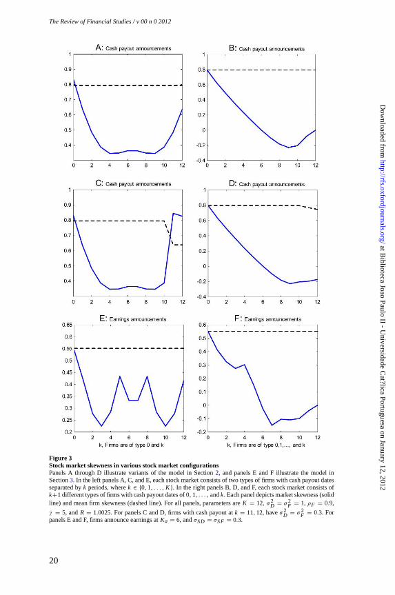
4.2 Skewness and cross-sectional heterogeneity in announcement eventsTo evaluate the effect of cross-sectional heterogeneity in event dates oncoskewness, I conduct two numerical experiments that simulate a variety ofstock market configurations. In all experiments and for simplicity, I assumeone firm per firm type. I use dollar returns because the model provides closed-form solutions for all relevant moments, but model simulations show that theresults hold for simple, percent returns as well. Figure3 presents the results.Panels A through D illustrate variants of the model in Section2, and panels Eand F illustrate the model in Section3. For each stock market configuration,I plot mean firm skewness (dashed line) and market skewness (solid line).For comparability with the empirical analysis, skewness is the third centeredmoment of returns normalized by the standard deviation cubed.
In the first experiment, reported in the left panels A, C, and E, each stockmarket is composed of two types of firms with cash payouts separated bykperiods, wherek ∈ {0,1, ..., K }. By varyingk, the two firms start off similar,become increasingly dissimilar, and end up similar again. I chooseK = 12so that each trading period represents one week and the time from 0 toKcorresponds to one calendar quarter. BecauseN = 2, this experiment exploresthe effect of cross-sectional heterogeneity ignoring theco-covterm.
In the second experiment, reported in the right panels B, D, and F, I allowa role for theco-covterm by having the number of firms in the stock marketgrow as heterogeneity across firms also changes. Each stock market is indexedby k, meaning it consists ofk + 1 firm types with cash payout dates at periods0,1, ..., andk. The period from 0 tok thus denotes an announcement seasonduring the window of time 0, ..., K .
In panel A, mean firm skewness is constant because with i.i.d. cash flowsfirm skewness does not depend on a firm’s payout date. Market skewnessis symmetric because having the second firm pay outk periods after thefirst firm or k periods before the first firm results in identical cross-sectionalheterogeneity. Coskewness can be very large and negative but never sufficientlyso in order to offset the individual skewness terms. Coskewness is particularlynegative when the two firms pay out at dates that are furthest apart becausethen the high volatility of the announcing firm contrasts the most with the con-temporaneously low expected return of the nonannouncing firm. In summary,the experiment suggests that theco-vol terms can significantly reduce marketskewness relative to firm-level skewness, but cannot generate negative marketskewness. This result is confirmed with many other parameterizations.
In panel B, mean firm skewness is also constant because each firm’sskewness does not depend on the payout date. Market skewness displays aflipped J-curve with respect tok. Fork = 0, there is only one firm type in the
19
at Biblioteca Joao Paulo II - U
niversidade Cat?lica Portuguesa on January 12, 2012
http://rfs.oxfordjournals.org/D
ownloaded from
The Review of Financial Studies / v 00 n 0 2012
Figure 3Stock market skewness in various stock market configurationsPanels A through D illustrate variants of the model in Section2, and panels E and F illustrate the model inSection3. In the left panels A, C, and E, each stock market consists of two types of firms with cash payout datesseparated byk periods, wherek ∈ {0,1, . . . , K }. In the right panels B, D, and F, each stock market consists ofk+1 different types of firms with cash payout dates of0,1, . . . , andk. Each panel depicts market skewness (solidline) and mean firm skewness (dashed line). For all panels, parameters areK = 12, σ2
D = σ2F = 1, ρF = 0.9,
γ = 5, andR = 1.0025.For panels C and D, firms with cash payout atk = 11,12, haveσ2D = σ2
F = 0.3. Forpanels E and F, firms announce earnings atKa = 6, andσSD = σSF = 0.3.
20
at Biblioteca Joao Paulo II - U
niversidade Cat?lica Portuguesa on January 12, 2012
http://rfs.oxfordjournals.org/D
ownloaded from

Skewness in Stock Returns: Reconciling the Evidence on Firm versus Aggregate Returns
stockmarket, and mean firm and market skewness are identical. Fork = 1,the stock market has two firm types, one with a cash payout at 0 and the otherat 1. This case is also present in panel A of the figure. Fork > 1, skewnessdrops faster than it did in panel A because of a negativeco-covterm. As morefirm types are added and the range of cash payout dates is widened, marketskewness becomes negative. The negative market skewness occurs despite thefact that mean firm skewness is positive. Market skewness remains negativeuntil the stock market consists of one firm of each type. When the stock marketconsists of one firm of each type, skewness is zero because every period looksthe same with equal aggregate stock market conditional mean and volatility ofreturns.
The result that skewness is zero when the stock market is composed of anequal number of firms announcing in each period is an artifact of the absenceof other forms of heterogeneity across firms. Assume, as way of an example,that firms with cash payouts atk = 11,12, have lower volatility of cash flowshocks. The model results are depicted in panels C and D of Figure3. Thedifferences to panels A and B are in the last two stock market configurationsof each panel, which contain one or both of these firm types. Loweringσ 2
D andσ 2
F implies lower announcement excess returns in the context of the model inSection2.4 Thesymmetry that exists in panel A is not perfect in panel C, butis still present. As for panel D, note that the lower volatility associated withfirms announcing atk = 11,12, and their associated lower expected returnscontribute to keeping skewness down and negative even when all firm typesare present in the market.
Finally, consider panels E and F. In general, adding earnings announcementevents produces similar observations to those of the cash payout model inpanels A and B. The plot in panel E shows a symmetric pattern for skewness,which as before results from the symmetry of event dates, and the plot in panelF shows a generally declining market skewness ask increases. As expected,panels E and F show that firm-level skewness is lower in the presence of theadditional event. This has implications for market skewness: with incompleteinformation, the numerical example shows that it is enough to have sevendifferent types of firms in order to generate negative market skewness, whereasin the complete information model of panels A and B, the same parametersrequire eight different firm types. From now on, I focus attention on the simplermodel of cash payouts and complete information.
The possibility that theco-covterm is responsible for the negative skewnessin the stock market is investigated further in Figure4. This figure plots market
4 Themotivation for allowing the additional firm heterogeneity comes fromCohen et al.(2007), who show thatfirms that made a preannouncement in the quarter have significantly lower announcement excess returns. Thisis to be expected as the preannouncement would have removed some of the uncertainty associated with firmearnings. Likewise, it would be expected that with correlated cash flows the firms announcing late in the quarterwould have lower announcement excess returns because some uncertainty would have been removed in theannouncements of other firms.
21
at Biblioteca Joao Paulo II - U
niversidade Cat?lica Portuguesa on January 12, 2012
http://rfs.oxfordjournals.org/D
ownloaded from

The Review of Financial Studies / v 00 n 0 2012
Figure 4Decomposing stock market skewnessEach stock market consists ofk + 1 different types of firms with cash payout dates of0,1, ..., andk as in panelB of Figure3. The figure depicts market skewness (solid) and its coskewness component termco-cov(dashed).Parameters areK = 12, σ2
D = σ2F = 1, ρF = 0.9, γ = 5, andR = 1.0025.
skewness (solid line) in each of the stock market configurations in panel B ofFigure3, as well as the respectiveco-covterm (dashed line) also standardizedby market volatility. A common property of the numerical examples studied,and of this one in particular, is that theco-cov term is the main driver ofnegative skewness in the stock market despite the small number of firms,consistent with evidence presented in Figure2. The symmetry of events inthe model implies that ask approachesK and market skewness goes to zero,the co-covterm turns positive and theco-vol terms turn negative. Theco-volterms are negative for largek because almost every periodt consists of anevent period with one firm with the highest conditional volatility (the one withan event att + 1) and all the others with low volatility possibly below theirrespective unconditional means.
A negativeco-covterm arises from asymmetric stock correlations in marketupturns versus market downturns. To show this, I followLongin and Solnik(2001) andAng and Chen(2002), and compute exceedance correlationsdefined as the correlation between a firm’s stock return and the market
22
at Biblioteca Joao Paulo II - U
niversidade Cat?lica Portuguesa on January 12, 2012
http://rfs.oxfordjournals.org/D
ownloaded from
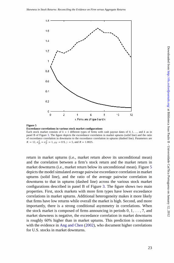
Skewness in Stock Returns: Reconciling the Evidence on Firm versus Aggregate Returns
Figure 5Exceedance correlations in various stock market configurationsEach stock market consists ofk + 1 different types of firms with cash payout dates of0,1, ..., and k as inpanel B of Figure3. The figure depicts the exceedance correlation in market upturns (solid line) and the ratioof exceedance correlation in downturns to the exceedance correlation in upturns (dashed line). Parameters areK = 12, σ2
D = σ2F = 1, ρF = 0.9, γ = 5, andR = 1.0025.
return in market upturns (i.e., market return above its unconditional mean)and the correlation between a firm’s stock return and the market return inmarket downturns (i.e., market return below its unconditional mean). Figure5depicts the model simulated average pairwise exceedance correlation in marketupturns (solid line), and the ratio of the average pairwise correlation indownturns to that in upturns (dashed line) across the various stock marketconfigurations described in panel B of Figure3. The figure shows two mainproperties. First, stock markets with more firm types have lower exceedancecorrelations in market upturns. Additional heterogeneity makes it more likelythat firms have low returns while overall the market is high. Second, and moreimportantly, there is a strong conditional asymmetry in correlations. Whenthe stock market is composed of firms announcing in periods 0, 1, . . . ,7, andmarket skewness is negative, the exceedance correlation in market downturnsis roughly 60% higher than in market upturns. This prediction is consistentwith the evidence inAng and Chen(2002), who document higher correlationsfor U.S. stocks in market downturns.
23
at Biblioteca Joao Paulo II - U
niversidade Cat?lica Portuguesa on January 12, 2012
http://rfs.oxfordjournals.org/D
ownloaded from

The Review of Financial Studies / v 00 n 0 2012
Figure 6Contribution of each trading period to stock market skewnessThe stock market consists of firms with cash payout dates of0,1, . . . , and7. The figure plots the componentof normalized skewness,E (Qt − E (Qt ))
3 /[E (Qt − E (Qt ))2]3/2, due to each trading period. Parameters are
K = 12, σ2D = σ2
F = 1, ρF = 0.9, γ = 5, andR = 1.0025.
It is also interesting to analyze which trading periods in the quartercontribute most toward overall skewness. Specifically, I am interested in theproperties of skewness with respect to the timing of the announcement season.Figure 6 presents a decomposition of the negative skewness for the stockmarket consisting of eight firm types, each firm type with a cash payoutat a different periodk, with k = 0, . . . ,7. The figure shows that mostnegative skewness occurs around the start of the event season when some firms’volatility spikes vis-a-vis that of others.
In the numerical examples above, I assume thatK = 12 so that there arealways 13 periods between any two events for the same firm. While the choiceis meant to identify each period as one week and each set of 13 periods asone quarter to match the regularity of the events studied, this choice is notinnocuous. TakingK = 0 means that payouts occur at every period, andin the model returns become unconditionally normally distributed with zeroskewness. More generally,K helps control the amount of firm heterogeneity inpayout dates. Small values ofK imply that there cannot be much heterogeneity
24
at Biblioteca Joao Paulo II - U
niversidade Cat?lica Portuguesa on January 12, 2012
http://rfs.oxfordjournals.org/D
ownloaded from

Skewness in Stock Returns: Reconciling the Evidence on Firm versus Aggregate Returns
and make it harder to generate negative aggregate skewness. For example,consider a stock market that consists of two firm types andK = 2. When onefirm-type has a payout event, the other will have one either next period or theperiod after. Because of the regularity of the payout events, both configurationswould imply the same level of market skewness. Because of the closeness ofthe announcements, market skewness would generally be positive.5
5. Empirical Evidence
I use daily return data on AMEX/NASDAQ/NYSE stocks from CRSP for theperiod between January 1, 1973, and December 31, 2009. I use the arithmeticholding period total return from CRSP, inclusive of dividends. I also obtainfrom CRSP dividend distribution information. I use variable DCLRDT toretrieve the date the board declares a distribution and variable DISTCD toselect ordinary dividends and notation of issuance. Information about earningsannouncement events is from the merged CRSP/Compustat quarterly file forthe period January 1, 1973, through June 30, 2009 (variable RDQ). Below,skewness is estimated using six months of daily return data. Firms are requiredto have complete return data within each semester to be included in the sample.
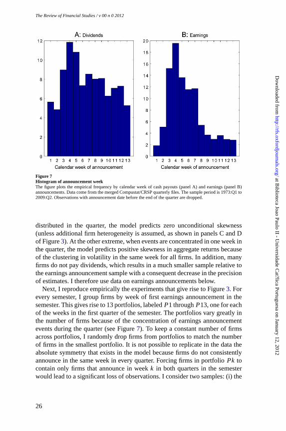
5.1 Cross-sectional heterogeneity in event datesI start by describing the cross-sectional dispersion in cash payout announce-ments and in earnings announcements. I am interested in the calendar weekof the announcement within the quarter. Figure7 plots the histograms of theannouncement week for cash payouts (panel A) and of the announcement weekfor earnings announcements (panel B).6 Cashpayouts are close to uniformlydistributed across the quarter. In contrast, and consistent with other studies(e.g., Chambers and Penman 1984; Kross and Schroeder 1984), earningsannouncements occur in seasons, being concentrated between weeks twoand eight in the calendar quarter and leaving the other half of the quarterwith less than 20% of the announcements. These patterns are consistentacross various subsamples and also across the various calendar quarters. Theevidence suggests that cross-sectional dispersion in payout dates may not beable to explain the negative skewness in aggregate returns, but that cross-sectional dispersion in earnings announcement events may explain the negativeskewness in aggregate returns. The reason is that when events are uniformly
5 Moreover, empirically, a largeK mayaffect the precision of the skewness estimates. In addition, two facts aboutthe timing of earnings announcements suggest looking at weekly periods. First, earnings announcements arefairly predictable (e.g.,Chambers and Penman 1984; Givoly and Palmon 1982). For quarterly announcements,Chambers and Penman estimate that for the representative firm the standard deviation of the actual earningsdate minus the estimated date is three to four calendar days. LettingK = 12 eliminatessome of the concernthat investors cannot predict the announcement date as well as they can in the model. Second, firms tend toannounce bad news on Fridays (e.g.,Damodaran 1989; Penman 1987). Letting K = 66 addsa concern forspecial weekdays that is absent in the model.
6 For earnings announcements, observations with an announcement date before the end of the quarter are dropped.
25
at Biblioteca Joao Paulo II - U
niversidade Cat?lica Portuguesa on January 12, 2012
http://rfs.oxfordjournals.org/D
ownloaded from
The Review of Financial Studies / v 00 n 0 2012
Figure 7Histogram of announcement weekThe figure plots the empirical frequency by calendar week of cash payouts (panel A) and earnings (panel B)announcements. Data come from the merged Compustat/CRSP quarterly files. The sample period is 1973:Q1 to2009:Q2. Observations with announcement date before the end of the quarter are dropped.
distributed in the quarter, the model predicts zero unconditional skewness(unless additional firm heterogeneity is assumed, as shown in panels C and Dof Figure3). At the other extreme, when events are concentrated in one week inthe quarter, the model predicts positive skewness in aggregate returns becauseof the clustering in volatility in the same week for all firms. In addition, manyfirms do not pay dividends, which results in a much smaller sample relative tothe earnings announcement sample with a consequent decrease in the precisionof estimates. I therefore use data on earnings announcements below.
Next, I reproduce empirically the experiments that give rise to Figure3. Forevery semester, I group firms by week of first earnings announcement in thesemester. This gives rise to 13 portfolios, labeledP1 throughP13, one for eachof the weeks in the first quarter of the semester. The portfolios vary greatly inthe number of firms because of the concentration of earnings announcementevents during the quarter (see Figure7). To keep a constant number of firmsacross portfolios, I randomly drop firms from portfolios to match the numberof firms in the smallest portfolio. It is not possible to replicate in the data theabsolute symmetry that exists in the model because firms do not consistentlyannounce in the same week in every quarter. Forcing firms in portfolioPk tocontain only firms that announce in weekk in both quarters in the semesterwould lead to a significant loss of observations. I consider two samples: (i) the
26
at Biblioteca Joao Paulo II - U
niversidade Cat?lica Portuguesa on January 12, 2012
http://rfs.oxfordjournals.org/D
ownloaded from
Skewness in Stock Returns: Reconciling the Evidence on Firm versus Aggregate Returns
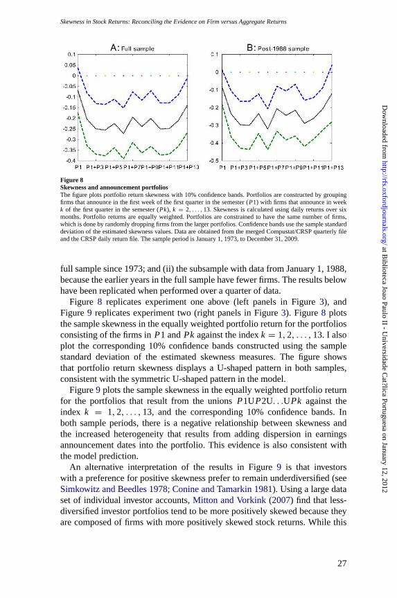
Figure 8Skewness and announcement portfoliosThe figure plots portfolio return skewness with10% confidence bands. Portfolios are constructed by groupingfirms that announce in the first week of the first quarter in the semester (P1) with firms that announce in weekk of the first quarter in the semester (Pk), k = 2, . . . ,13. Skewness is calculated using daily returns over sixmonths. Portfolio returns are equally weighted. Portfolios are constrained to have the same number of firms,which is done by randomly dropping firms from the larger portfolios. Confidence bands use the sample standarddeviation of the estimated skewness values. Data are obtained from the merged Compustat/CRSP quarterly fileand the CRSP daily return file. The sample period is January 1, 1973, to December 31, 2009.
full sample since 1973; and (ii) the subsample with data from January 1, 1988,because the earlier years in the full sample have fewer firms. The results belowhave been replicated when performed over a quarter of data.
Figure 8 replicates experiment one above (left panels in Figure3), andFigure9 replicates experiment two (right panels in Figure3). Figure8 plotsthe sample skewness in the equally weighted portfolio return for the portfoliosconsisting of the firms inP1 andPk against the indexk = 1,2, . . . ,13. I alsoplot the corresponding 10% confidence bands constructed using the samplestandard deviation of the estimated skewness measures. The figure showsthat portfolio return skewness displays a U-shaped pattern in both samples,consistent with the symmetric U-shaped pattern in the model.
Figure9 plots the sample skewness in the equally weighted portfolio returnfor the portfolios that result from the unionsP1UP2U. . .UPk against theindex k = 1,2, . . . ,13, and the corresponding 10% confidence bands. Inboth sample periods, there is a negative relationship between skewness andthe increased heterogeneity that results from adding dispersion in earningsannouncement dates into the portfolio. This evidence is also consistent withthe model prediction.
An alternative interpretation of the results in Figure9 is that investorswith a preference for positive skewness prefer to remain underdiversified (seeSimkowitz and Beedles 1978;Conine and Tamarkin 1981). Using a large dataset of individual investor accounts,Mitton and Vorkink(2007) find that less-diversified investor portfolios tend to be more positively skewed because theyare composed of firms with more positively skewed stock returns. While this
27
at Biblioteca Joao Paulo II - U
niversidade Cat?lica Portuguesa on January 12, 2012
http://rfs.oxfordjournals.org/D
ownloaded from

The Review of Financial Studies / v 00 n 0 2012
Figure 9Skewness and announcement portfoliosThe figure plots portfolio return skewness with10% confidence bands. Portfolios are constructed by groupingfirms that announce between the first week of the first quarter in the semester (P1) and weekk of the first quarterin the semester (Pk), k = 2, ...,13. Skewness is calculated using daily returns over six months. Portfolio returnsare equally weighted. Portfolios are constrained to have the same number of firms, which is done by randomlydropping firms from the larger portfolios. Confidence bands use the sample standard deviation of the estimatedskewness values. Data are obtained from the merged Compustat/CRSP quarterly file and the CRSP daily returnfile. The sample period is January 1, 1973, to December 31, 2009.
Figure 10Mean firm skewness and announcement portfoliosThe figure plots the mean firm return skewness with10% confidence bands. Portfolios are constructed bygrouping firms that announce between the first week of the first quarter in the semester (P1) and weekk of thefirst quarter in the semester (Pk), k = 2, . . . ,13. Firm skewness is calculated using daily returns over six months.PortfoliosPk are constrained to have the same number of firms as in Figure3. Confidence bands use the samplestandard deviation of the estimated skewness values. Data are obtained from the merged Compustat/CRSPquarterly file and the CRSP daily return file. The sample period is January 1, 1973, to December 31, 2009.
alternative interpretation is plausible, it does not apply to the announcement-week portfolios constructed here. Figure10 shows that the larger (and morediversified) portfolios in Figure9 have approximately the same mean firmskewness as the smaller portfolios. This alternative interpretation is also notconsistent with the evidence I present next.
28
at Biblioteca Joao Paulo II - U
niversidade Cat?lica Portuguesa on January 12, 2012
http://rfs.oxfordjournals.org/D
ownloaded from

Skewness in Stock Returns: Reconciling the Evidence on Firm versus Aggregate Returns
Figure 11Skewness and calendar weekThe figure plots the weekly component of market skewness with10%confidence bands. Skewness is calculatedusing daily returns over six months. Portfolio returns are equally weighted. Confidence bands use the samplestandard deviation of the estimated skewness values. Data are obtained from the CRSP daily return file. Thesample period is January 1, 1973, to December 31, 2009.
Finally, I present evidence of how the earnings announcement season isrelated to skewness. I decompose market skewness computed using six monthsof data into its weekly components. The decomposition guarantees that addingup the weekly components yields the market skewness for the six-monthperiod. Recalling panel B of Figure7, an earnings announcement season startsshortly after the beginning of every quarter. Figure11 shows that an earningsannouncement season is also when skewness has its most negative compo-nents during the quarter, consistent with the model prediction illustrated inFigure6.
There are two main caveats regarding the evidence presented and the modelpredictions. First, in Figure9, skewness strictly declines withk, whereas in themodel, when all firm types are allowed, skewness becomes zero. This propertyof the model is the result of (i) limiting heterogeneity across firms to the eventdate (see panel D of Figure3); and (ii) imposing that firms always announcein the same calendar week in every quarter, which is not validated in the data.Second, in both Figures8 and9, point estimates of portfolio return skewnessare negative. One possible explanation for the negative portfolio skewness isthat even the firms in the same portfolioPk differ in the week of earningsannouncement in the second quarter of the semester. Another explanation isthat the cross-sectional heterogeneity in events is not subsumed in the cross-sectional heterogeneity of earnings announcement events. Finally, it could bethe case that firm returns are exposed to a common factor that is negativelyskewed. I return to this last point in subsection5.3.
29
at Biblioteca Joao Paulo II - U
niversidade Cat?lica Portuguesa on January 12, 2012
http://rfs.oxfordjournals.org/D
ownloaded from
TheReview of Financial Studies / v 00 n 0 2012
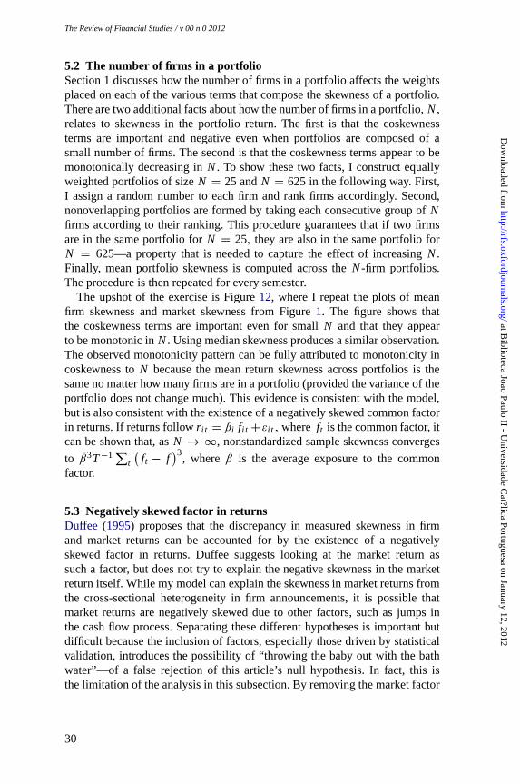
5.2 The number of firms in a portfolioSection 1 discusses how the number of firms in a portfolio affects the weightsplaced on each of the various terms that compose the skewness of a portfolio.There are two additional facts about how the number of firms in a portfolio,N,relates to skewness in the portfolio return. The first is that the coskewnessterms are important and negative even when portfolios are composed of asmall number of firms. The second is that the coskewness terms appear to bemonotonically decreasing inN. To show these two facts, I construct equallyweighted portfolios of sizeN = 25 andN = 625 in the following way. First,I assign a random number to each firm and rank firms accordingly. Second,nonoverlapping portfolios are formed by taking each consecutive group ofNfirms according to their ranking. This procedure guarantees that if two firmsare in the same portfolio forN = 25, they are also in the same portfolio forN = 625—a property that is needed to capture the effect of increasingN.Finally, mean portfolio skewness is computed across theN-firm portfolios.The procedure is then repeated for every semester.
The upshot of the exercise is Figure12, where I repeat the plots of meanfirm skewness and market skewness from Figure1. The figure shows thatthe coskewness terms are important even for smallN and that they appearto be monotonic inN. Using median skewness produces a similar observation.The observed monotonicity pattern can be fully attributed to monotonicity incoskewness toN because the mean return skewness across portfolios is thesame no matter how many firms are in a portfolio (provided the variance of theportfolio does not change much). This evidence is consistent with the model,but is also consistent with the existence of a negatively skewed common factorin returns. If returns followri t = βi fi t + εi t , where ft is the common factor, itcan be shown that, asN → ∞, nonstandardized sample skewness converges
to β3T−1∑t
(ft − f
)3, where β is the average exposure to the common
factor.
5.3 Negatively skewed factor in returnsDuffee (1995) proposes that the discrepancy in measured skewness in firmand market returns can be accounted for by the existence of a negativelyskewed factor in returns. Duffee suggests looking at the market return assuch a factor, but does not try to explain the negative skewness in the marketreturn itself. While my model can explain the skewness in market returns fromthe cross-sectional heterogeneity in firm announcements, it is possible thatmarket returns are negatively skewed due to other factors, such as jumps inthe cash flow process. Separating these different hypotheses is important butdifficult because the inclusion of factors, especially those driven by statisticalvalidation, introduces the possibility of “throwing the baby out with the bathwater”—of a false rejection of this article’s null hypothesis. In fact, this isthe limitation of the analysis in this subsection. By removing the market factor
30
at Biblioteca Joao Paulo II - U
niversidade Cat?lica Portuguesa on January 12, 2012
http://rfs.oxfordjournals.org/D
ownloaded from

Skewness in Stock Returns: Reconciling the Evidence on Firm versus Aggregate Returns
Figure 12Skewness in portfolios of varying sizeThe figure plots mean skewness in daily returns from portfolios of sizeN. Skewness is computed using equallyweighted portfolio returns and six months of daily data. The portfolios are constructed by randomly rankingthe firms and then grouping them. If two firms are in the same portfolio whenN = 25, then they will alsobe in the same portfolio forN = 625. The dash-dotted line plots firm-level skewness. The solid line, labeledMarket, plots skewness of equally weighted returns of all firms in CRSP. The sample period is January 1, 1973,to December 31, 2009.
from firm returns, it assumes that the skewness in the market factor is unrelatedto the mechanism proposed in the article.
I remove one common factor from returns for the following reasons. First,the Appendix shows that the model is a one-factor model. Second, the marketfactor may capture the effect of peso problems or jumps in (common factorsin) cash flows that would arise in a more general model, whereas a secondfactor may capture the skewness induced by cross-sectional heterogeneityin firm events. Third,Engle and Mistry(2007) suggest that the ICAPM isinconsistent with priced risk factors that do not display asymmetric volatilityor for which time aggregation changes the sign of skewness. In their article,the market factor is negatively skewed across all frequencies. The size andmomentum factors are negatively skewed at high frequencies but positivelyskewed at lower frequencies, and the book-to-market factor is positively
31
at Biblioteca Joao Paulo II - U
niversidade Cat?lica Portuguesa on January 12, 2012
http://rfs.oxfordjournals.org/D
ownloaded from
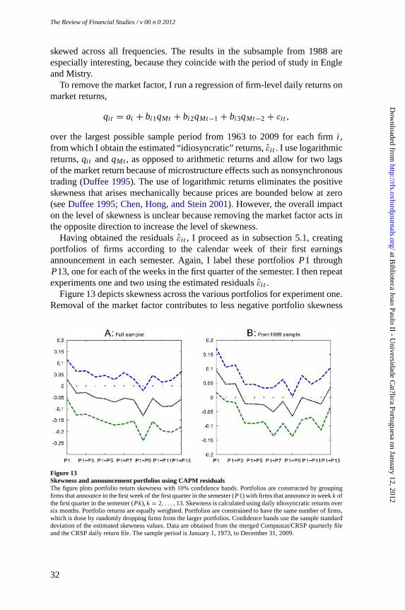
The Review of Financial Studies / v 00 n 0 2012
skewed across all frequencies. The results in the subsample from 1988 areespecially interesting, because they coincide with the period of study in Engleand Mistry.
To remove the market factor, I run a regression of firm-level daily returns onmarket returns,
qit = ai + bi 1qMt + bi 2qMt−1 + bi 3qMt−2 + εi t ,
over the largest possible sample period from 1963 to 2009 for each firmi ,from which I obtain the estimated “idiosyncratic” returns,εi t . I use logarithmicreturns,qit andqMt , as opposed to arithmetic returns and allow for two lagsof the market return because of microstructure effects such as nonsynchronoustrading (Duffee 1995). The use of logarithmic returns eliminates the positiveskewness that arises mechanically because prices are bounded below at zero(seeDuffee 1995;Chen, Hong, and Stein 2001). However, the overall impacton the level of skewness is unclear because removing the market factor acts inthe opposite direction to increase the level of skewness.
Having obtained the residualsεi t , I proceed as in subsection5.1, creatingportfolios of firms according to the calendar week of their first earningsannouncement in each semester. Again, I label these portfoliosP1 throughP13, one for each of the weeks in the first quarter of the semester. I then repeatexperiments one and two using the estimated residualsεi t .
Figure13depicts skewness across the various portfolios for experiment one.Removal of the market factor contributes to less negative portfolio skewness
Figure 13Skewness and announcement portfolios using CAPM residualsThe figure plots portfolio return skewness with10% confidence bands. Portfolios are constructed by groupingfirms that announce in the first week of the first quarter in the semester (P1) with firms that announce in weekk ofthe first quarter in the semester (Pk), k = 2, . . . ,13. Skewness is calculated using daily idiosyncratic returns oversix months. Portfolio returns are equally weighted. Portfolios are constrained to have the same number of firms,which is done by randomly dropping firms from the larger portfolios. Confidence bands use the sample standarddeviation of the estimated skewness values. Data are obtained from the merged Compustat/CRSP quarterly fileand the CRSP daily return file. The sample period is January 1, 1973, to December 31, 2009.
32
at Biblioteca Joao Paulo II - U
niversidade Cat?lica Portuguesa on January 12, 2012
http://rfs.oxfordjournals.org/D
ownloaded from

Skewness in Stock Returns: Reconciling the Evidence on Firm versus Aggregate Returns
Figure 14Skewness and announcement portfolios using CAPM residualsThe figure plots portfolio return skewness with10% confidence bands. Portfolios are constructed by groupingfirms that announce between the first week of the first quarter in the semester (P1) and weekk of the first quarterin the semester (Pk), k = 2, . . . ,13. Skewness is calculated using daily idiosyncratic returns over six months.Portfolio returns are equally weighted. Portfolios are constrained to have the same number of firms, which isdone by randomly dropping firms from the larger portfolios. Confidence bands use the sample standard deviationof the estimated skewness values. Data are obtained from the merged Compustat/CRSP quarterly file and theCRSP daily return file. The sample period is January 1, 1973, to December 31, 2009.
as compared with Figure8. In the full sample, portfolio skewness is alwaysinsignificant, though the point estimate forP1 is positive. However, thesymmetry present in Figure8 is lost. In the subsample with post-1988 data,not only is the skewness inP1 significantly positive, but there also is a moresymmetric relation in the point estimates. It is possible that the greater numberof firms listed in this subsample is contributing to the better results. Figure14 depicts the results for experiment two. Again, compared with Figure9,portfolio skewness is higher after the removal of the market factor. Consistentwith the model, there are now several positive point estimates for portfolioskewness and there also is a more pronounced flattening of the skewness curveask increases.
5.4 Timing of announcementsAcharya et al. (forthcoming) propose a model of endogenous information re-leases where each firm has positively skewed returns, but the stock market maydisplay negative conditional skewness when firms cluster their announcementsaround the release of bad economy-wide news. Despite the similarity of someof the predictions, the information events that Acharya et al. study are verydifferent in nature from earnings announcement events modeled here. Theirsis a model of voluntary disclosures, which have a median occurrence of zero ina quarter (Bhojraj, Li, and Yang 2010), whereas earnings announcements aremandatory.
To further distinguish the two hypotheses, I construct the distribution ofearnings announcements conditioning on market movements. According to
33
at Biblioteca Joao Paulo II - U
niversidade Cat?lica Portuguesa on January 12, 2012
http://rfs.oxfordjournals.org/D
ownloaded from

The Review of Financial Studies / v 00 n 0 2012
Figure 15Stationary conditional cumulative distributions of earnings announcementsPanel A classifies market upturns (downturns) as quarters preceded by a CRSP value-weighted return above(below) the historical median. Panel B classifies market upturns (downturns) as quarters preceded by a CRSPvalue-weighted return above the historical 75th percentile (below the 25% percentile). The distribution depictedusing a dashed line conditions on market upturns, and the distribution depicted using a solid line conditions onmarket downturns. Data on earnings announcements come from the merged Compustat/CRSP quarterly files.The sample period is 1973:Q1 to 2009:Q2. Observations with announcement dates before the end of the quarterare dropped.
Acharya et al., bunching of earnings announcements is to be expected aftermarket downturns, relative to market upturns. I take the monthly CRSP value-weighted return (including distributions) prior to every quarter and labelmarket upturns as those quarters that follow a return above the median andmarket downturns as those quarters that follow a return below the median.I repeat the analysis using as cutoffs the 75th percentile and the 25th percentile,respectively. The results are robust to using monthly market returns and to us-ing contemporaneous returns. Conditional on the market return, I construct thetransition matrix of earnings announcements by keeping track of when firmsannounced in the previous and current quarters. These transition matrices haveno zero elements and thus have a unique stationary distribution (seeLjungqvistand Sargent 2000). The stationary conditional cumulative distributions aredepicted in Figure15. The distribution depicted using a dashed (solid) lineconditions on market upturns (downturns). There is no apparent bunching aftermarket downturns and, contrary to Acharya et al., a slightly larger fraction offirms tend to announce at the beginning of the quarter after market upturns.
6. Conclusion
The main contribution of this article is to model and provide evidence ona new source of negative skewness in market returns. This source consists
34
at Biblioteca Joao Paulo II - U
niversidade Cat?lica Portuguesa on January 12, 2012
http://rfs.oxfordjournals.org/D
ownloaded from

Skewness in Stock Returns: Reconciling the Evidence on Firm versus Aggregate Returns
of the cross-sectional heterogeneity in the timing of earnings announcementevents. The article develops a simple model to capture the observed changesin volatility and mean returns around cash payout and earnings announcementevents. The model shows that periodicity in these events gives rise to condi-tional heteroscedasticity and positive skewness in firm returns consistent withthe data. The model also shows that heterogeneity in the timing of these eventscan lead to negative skewness in market returns despite the positive skewnessin firm returns. The negative skewness in market returns in the model is furthershown to be caused by stock correlations that are asymmetrically higher inmarket downturns. These model predictions are consistent with evidence basedon the cross-sectional dispersion of earnings announcement events.
The results in this article can be informative to the literature on rare disastersthat tries to explain the equity premium puzzle and also predicts negativeskewness in aggregate stock returns (e.g.,Rietz 1988;Barro 2006). Like thisarticle,Chang, Christoffersen, and Jacobs(2009) present evidence suggestivethat aggregate skewness may not be due to jump risk. Future research shoulddevelop structural models nesting several hypotheses to better identify thesources of negative skewness in aggregate returns.
The results in this article are also pertinent to the large literature that triesto model the dynamics of aggregate return volatility. The model predictsthat aggregate return volatility is partly explained by the cross-sectionalheterogeneity of firm-level volatility. Testing this prediction is left for futureresearch.
Appendix A: Proofs
ThisAppendix collects the proofs of the propositions in the text.
Proof of Proposition 1: Guess that equilibrium stock returns are conditionally normal with
Qk+1t+1 |t ∼ N
(μk, σ2
k
).
Therepresentative investor solves (3), subject to Equations (4) and (5). The problem yields thefamiliar first-order necessary and sufficient condition,
θt =μk
γ σ2k
.
Imposingthe market clearing condition that the representative investor holds all shares,θt = 1,gives Equation (9),μk = γ σ2
k . Using Equation (9), and assuming without loss of generality thattime t + 1 corresponds to a payout period, it is possible to write the following set of equilibriumconditions:
PKt = R−1
[−γ σ2
K + Et
[P0
t+1 + Dt+1
]]
PK−1t−1 = R−1
[−γ σ2
K−1 + Et−1
[PK
t
]]
. . .
35
at Biblioteca Joao Paulo II - U
niversidade Cat?lica Portuguesa on January 12, 2012
http://rfs.oxfordjournals.org/D
ownloaded from

TheReview of Financial Studies / v 00 n 0 2012
P0t−K = R−1
[−γ σ2
0 + Et−K
[P1
t−K+1
]]
PKt−K−1 = R−1
[−γ σ2
K + Et−K−1[Pt−K + Dt−K
]].
Assuming a stationary solution to this system of stochastic difference equations, recursivesubstitution yields Equation (7) in the proposition.
After constructing equilibrium returns from the price function (see Equation (10)), it isstraightforward to show that the values forpk obey the recursion
μk ≡ Et
[Qk+1
t+1
]= pk+1 − Rpk,
which can be solved to yield Equation (8). Stationarity implies that for anyk, Et
[Qk+1+K
t+1
]=
Et
[Qk
t+1
]. �
Proof of Corollary 1: Given Equation (7), construct returns (10). It is then straightforward toderive the conditional variance of stock returns. The conditional variance is increasing and convexin k, becauseR−(K+1−k) is increasing and convex ink and, withρF/R < 1, Γk is also increasingand convex ink. The conditional mean return is proportional to the conditional return variance (seeEquation (9)) and thus is also increasing and convex ink. �
Proof of Corollary 2: Using the definition off (Q), the unconditional mean stock return is
E(Qt+1
)=
1
K + 1
K∑
k=0
Ek(Qt+1
)=
1
K + 1
K∑
k=0
μk.
Theunconditional variance in stock returns is
V ar(Qt+1
)=
1
K + 1
K∑
k=0
∫ (Q − E
(Qt+1
))2φ(
Q; μk, σ2k
)dQ
=1
K + 1
K∑
k=0
∫ (Q − μk + μk − E
(Qt+1
))2φ(
Q; μk, σ2k
)dQ
=1
K + 1
K∑
k=0
(σ2
k +(μk − E
(Qt+1
))2)
.
Finally, unconditional skewness is
E[(
Q − E(Qt+1
))3]
=1
K + 1
K∑
k=0
∫ (Q − E
(Qt+1
))3φ(
Q; μk, σ2k
)dQ
=1
K + 1
K∑
k=0
∫ (Q − μk + μk − E
(Qt+1
))3φ(
Q; μk, σ2k
)dQ
=1
K + 1
K∑
k=0
[(μk − E
(Qt+1
))3 + 3σ2k(μk − E
(Qt+1
))].
Thethird equality uses∫
(Q − μk) φ(
Q; μk, σ2k
)dQ = 0 and the fact that skewness is zero for
a normal variable,∫
(Q − μk)3 φ(
Q; μk, σ2k
)dQ = 0. The second term under the summation
36
at Biblioteca Joao Paulo II - U
niversidade Cat?lica Portuguesa on January 12, 2012
http://rfs.oxfordjournals.org/D
ownloaded from

Skewness in Stock Returns: Reconciling the Evidence on Firm versus Aggregate Returns
signcan be manipulated to yield the expression in the corollary by noting that
μk − E(Qt+1
)=
1
K + 1
K∑
j =0, j 6=k
(μk − μ j
),
andgrouping terms together under the last summation sign. �
Proof of Proposition 3: Guess prices to be
Pkt = pk + Γk Et (Ft ) + R−(K+1−k)
k−1∑
j =0
Et
(εDt− j
),
for all k. Obviously fork ≥ Ka, the expectations operators drop out because the shocks are in theinvestors’ information set. Excess stock returns are
Qkt = Pk
t − RPk−1t−1
= pk + Γk Et (Ft ) + R−(K+1−k)k−1∑
j =0
Et
(εDt− j
)
−R
pk−1 +(ρF/R)K+2−k
1 − (ρF/R)K+1Et−1
(Ft−1
)+ R−(K+2−k)
k−2∑
j =0
Et−1
(εDt−1− j
)
,
for any period 1≤ k ≤ Ka − 1. Because
Et (Ft ) = ρF Et−1(Ft−1
)+ Et
(εFt
)
= ρF Et−1(Ft−1
)+
σ2F
σ2F + σ2
SF
SFt ,
theexpression for returns reduces to
Qkt = pk − Rpk−1 + Γk
σ2F
σ2F + σ2
SF
SFt + R−(K+1−k) σ2
D
σ2D + σ2
SD
SDt .
Above, I used
Et(Ft−1
)= Et−1
(Ft−1
), Et
(εDt−1
)= Et−1
(εDt−1
), . . . , Et
(εDt−k+1
)= Et−1
(εDt−k+1
),
knowing that timet signals are not informative aboutt − n shocks for anyn > 0. For periodk = Ka,
Qkt = Pk
t − RPk−1t−1
= pk + Γk Ft + R−(K+1−k)k−1∑
j =0
εDt− j
−R
pk−1 +(ρF/R)K+2−k
1 − (ρF/R)K+1Et−1
(Ft−1
)+ R−(K+2−k)
k−2∑
j =0
Et−1
(εDt−1− j
)
,
37
at Biblioteca Joao Paulo II - U
niversidade Cat?lica Portuguesa on January 12, 2012
http://rfs.oxfordjournals.org/D
ownloaded from

TheReview of Financial Studies / v 00 n 0 2012
or rearranging,
Qkt = pk − Rpk−1 + ΓkρF
[Ft−1 − Et−1
(Ft−1
)]+ ΓkεF
t
+R−(K+1−k)
εDt +
k−2∑
j =0
[εDt−1− j − Et−1
(εDt−1− j
)]
.
Finally, for k > Ka, returns take the same form with the same conditional moments as inCorollary1.
It is now easy to construct conditional return moments. For variance, and for any period 1≤k ≤ Ka − 1,
Vart−1
(Qk
t
)= Γ2
kσ4
F
σ2F + σ2
SF
+ R−2(K+1−k) σ4D
σ2D + σ2
SD
,
which is increasing and convex ink. For periodk = Ka,
Vart−1
(Qk
t
)= Γ2
kρ2F Vart−1
[Ft−1 − Et−1
(Ft−1
)]+ Γ2
kσ2F
+R−2(K+1−k)
σ2
D +k−2∑
j =0
Vart−1
[εDt−1− j − Et−1
(εDt−1− j
)]
.
In addition,
Et−1
(εDt−1
)=
σ2D
σ2D + σ2
SD
SDt−1,
Vart−1
(εDt−1
)=
σ2Dσ2
SD
σ2D + σ2
SD
,
and
Vart−1,Ka−1[Ft−1 − Et−1
(Ft−1
)]
= Vart−1,Ka−1
[εFt−1 − Et−1
(εFt−1
)+ ... + ρ
Ka−2F
(εFt−Ka+1 − Et−Ka+1
(εFt−Ka+1
))]
=σ2
Fσ2SF
σ2F + σ2
SF
{1 + ρ2
F + ... + ρKa−2F
}.
For k ≤ Ka,
Vart−1
(Qk
t
)> Vart−2
(Qk−1
t−1
).
Furthermore,
Vart−1
(QKa
t
)> Vart
(QKa+1
t+1
)
is possible if the arrival of information from past shocks is relevant enough. In that case, thepath of conditional variance displays two distinct periods of convexity. Finally, knowing that
μk = γ Vark(
Qk+1t+1
), it is possible to recover the constantspk verifying that the price function
above is an equilibrium price. �
38
at Biblioteca Joao Paulo II - U
niversidade Cat?lica Portuguesa on January 12, 2012
http://rfs.oxfordjournals.org/D
ownloaded from

Skewness in Stock Returns: Reconciling the Evidence on Firm versus Aggregate Returns
Calculationsin the many-firm case: Here, I derive several unconditional moments of aggregatereturns including skewness, which is given in the main text in Equation (15). Using the definitionof f (Q), for a stock market composed ofN firms, the unconditional mean stock return is
E(QMt+1
)=
1
K + 1
K∑
k=0
Ek(QMt+1
)=
1
K + 1
K∑
k=0
1
N
N∑
i =1
μik.
Theunconditional variance in stock returns is
V ar(QMt+1
)=
1
K + 1
K∑
k=0
∫ (Q − E
(Qt+1
))2φ(
Q; μMk , σ2
M,k
)dQ
=1
K + 1
K∑
k=0
∫ (Q − μM
k + μMk − E
(Qt+1
))2φ(
Q; μMk , σ2
M,k
)dQ
=1
K + 1
K∑
k=0
(σ2
M,k +(μM
k − E(Qt+1
))2)
.
Unconditionalskewness is
E[(QMt − E (QMt ))
3]
=1
K + 1
K∑
k=0
∫(Q − E (Q))3 φ (Q; k) dQ
=1
K + 1
K∑
k=0
∫ ((Q − μM
k
)3+(μM
k − E (Q))3)
φ (Q; k) dQ
+3
K + 1
K∑
k=0
∫ (Q − μM
k
)2 (μM
k − E (Q))
φ (Q; k) dQ
+3
K + 1
K∑
k=0
∫ (Q − μM
k
) (μM
k − E (Q))2
φ (Q; k) dQ,
or
E[(QMt − E (QMt ))
3]
=1
K + 1
K∑
k=0
(μM
k − E (Q))3
+3
K + 1
K∑
k=0
(μM
k − E (Q))
σ2M,k.
Expressingmarket returns as a sum of firm-level returns leads to
=1
N3
N∑
i =1
E[(Qi t − E (Qi t ))
3]
+3
K + 1
1
N3
K∑
k=0
N∑
i =1
N∑
i ′ 6=i
(μi
k − E (Qi ))2 (
μi ′k − E
(Qi ′
))
+3
K + 1
1
N3
K∑
k=0
N∑
i =1
(μi
k − E (Qi )) N∑
i ′ 6=i
σ2i ′k
+6
K + 1
1
N3
K∑
k=0
N∑
i =1
N∑
i ′>i
N∑
l>i ′
(μi
k − E (Qi )) (
μi ′k − E
(Qi ′
)) (μl
k − E (Ql ))
.
39
at Biblioteca Joao Paulo II - U
niversidade Cat?lica Portuguesa on January 12, 2012
http://rfs.oxfordjournals.org/D
ownloaded from

TheReview of Financial Studies / v 00 n 0 2012
Appendix B: Model with Correlated Cash Flows
In the correlated cash flow case, firmi ’s persistent dividend factor isFi t = ρFi Fi t−1 + εFi t ,
0 ≤ ρFi ≤ 1, with εFi t ∼ N
(0,σ2
Fi
), and the transitory component isεD
i t ∼ N(0,σ2
Di
). For
any two firmsi and i ′, E[εDi t εD
i ′t−s
]= σ D
i i ′ and E[εFi t ε
Fi ′t−s
]= σ F
i i ′ whens = 0, and zero
otherwise. I am interested in the case in which shocks have one or more common components thataffect the cash flows of all firms in the economy in the same direction,σ D
i i ′ , σFi i ′ ≥ 0.For simplicity,
E[εDi t εF
i ′t−s
]= 0 for any two firmsi andi ′ andanys. As in the main text, all dividend shocks
are homoscedastic.Denote byQk
t =(
Qk11t , ..., Q
kNNt
)ᵀthecolumn vector of timet stock returns. The superscriptk
indicates that firms of typek (if there are any) announce at timet . Again, with fixed heterogeneityin firm announcements,k is a sufficient statistic for the distribution of firms att .
Assuming that returns are jointly conditionally normal,
Qk+1t+1 |t ∼ N (μk, Vk) ,
theinvestors’ problem yields the first-order necessary and sufficient condition,
θt = γ −1V−1k μk.
Imposingthe equilibrium condition that the representative investor holds all shares in the market,θt = 1, givesμk = γ Vk1.
Following the steps of the proof of Proposition1 and assuming stationarity yields theequilibrium price function for firmi :
Pkii t = p
kii + Γki Fi t + R−(K+1−ki )
ki −1∑
j =0
εDi,t− j .
Theexpression for the constantspkii < 0 is the same as in Equation (8).
To solve for the equilibrium values of{μk, Vk}k, use the price function above to express excessreturns as
Qkii t = p
kii − Rp
ki −1i + Γki ε
Fi t + R−(K+1−ki )εD
i t ,
for anyki . Then, the elements ofVk are
σ2i k ≡ Vart
[Q
ki +1i t+1
]= Γ2
ki +1σ2Fi + R−2(K−ki )σ2
Di .
σi i ′,k ≡ Covt
[Q
ki +1i t+1 , Q
ki ′+1i ′t+1
]= Γki +1Γki ′+1σ F
i i ′ + R−(2K−ki −ki ′
)σ D
i i ′ .
For each firmi , the conditional mean and volatility of the stock return increase monotonically andare convex inki , all else equal. As in the uncorrelated cash flow case, the conditional stock returnvariance increases withki , all else equal.
In this model, as in the uncorrelated cash flow case, the stock market equilibrium has a
conditional CAPM representation. Letα ≡ 1/N, and write QkMt = α
ᵀQ
kt . Then, μM
k ≡
Et
[Qk+1
Mt+1
]= α
ᵀμk andσ2
M,k ≡ Et
[(Qk+1
Mt+1 − μMk
)2]
= αᵀ
Vkα. Then, usingμk = γ Vk1
gives
μk = βkμMk ,
whereβk ≡ Covk
(Qk
t , QkMt
)/σ2
M,k andαᵀβk = 1.
40
at Biblioteca Joao Paulo II - U
niversidade Cat?lica Portuguesa on January 12, 2012
http://rfs.oxfordjournals.org/D
ownloaded from

Skewness in Stock Returns: Reconciling the Evidence on Firm versus Aggregate Returns
If firm i has a high expected return around its announcement event, it must also be thatβ ik
is high around the event. This systematic risk is driven by the volatility associated with theinformation flow in common factors. For example, ifFi t = Ft for all t and i , andσ D
i i ′ = 0,then the economy has only one common factor, which is persistent. Shocks to this commonfactor, εF
t , affect stock returns of firms differently depending on how far each firm is fromits respective payout event. This timing explains the dynamics in the conditional stock returnmoments because proximity to a payout event determines the impact of (systematic) informationon returns. Consistent with this model prediction,Patton and Verardo(2010) show that dailyfirm betas increase by an economically and statistically significant amount around earningsannouncement events.
For comparability with the results in the main text, I present here the stochastic discount factorin the general case:
mk+1t+1 = γ exp
[−γ 1′μk+1 − γ 1′εk+1
t+1
],
where μk+1 is the vector of conditional mean returns andεk+1t+1 is the vector of common
innovations to the transitory and persistent dividend shocks with varianceVk+1. The cross-sectional dispersion of firm events determinesVk+1.
After deriving the equilibrium conditional distribution of stock returns, it is straightforward toderive the equilibrium unconditional distribution following the same steps as in the main text. ForK ≥ 1, the unconditional distribution of stock returns for firmi is a mixture of normals distributionwith density
f(
Qi)
=1
K + 1
K∑
k=0
φ(
Qi ; μik, σ2
i k
),
whereφ (.) is the normal density function, and forK = 0, returns are unconditionally normallydistributed. The expressions for the unconditional mean and variance of stock returns and theunconditional skewness in stock returns are the same as in the main text. With correlated cashflows, it is not possible to sign skewness because whenki changes,other firms’ event time, sayki ′ , also changes, which may lead to nonmonotonicity in the conditional return covariance betweeni andi ′ andhence in conditional mean returns for firmi . However, in numerical examples studied,this effect is dominated and firm-level skewness is positive.
The unconditional distribution of aggregate market returns is a mixture of normals distributionwith
f (QM ) =1
K + 1
K∑
k=0
φ(
QM ; μMk , σ2
M,k
),
andskewness in aggregate stock returns is as in Equation (15) plus the following term:
6
K + 1
1
N3
K∑
k=0
(μM
k − E (QM )) N∑
i =1
∑
i ′>i
σi i ′,k.
This term is likely to be positive because the return covariance is likely to be highest at eventdatesk, where mean returnsμM
k arealso likely to be higher. Hence, in the correlated cash flowcase, market skewness tends to be higher than in the uncorrelated case and there tends to beless conditional asymmetry in stock return correlations. However, numerical examples show thatqualitatively the results in the main text apply also to this more general model.
41
at Biblioteca Joao Paulo II - U
niversidade Cat?lica Portuguesa on January 12, 2012
http://rfs.oxfordjournals.org/D
ownloaded from

TheReview of Financial Studies / v 00 n 0 2012
ReferencesAcharya, V., P. DeMarzo, and I. Kremer. Forthcoming. Endogenous Information Flows and the Clustering ofAnnouncements.American Economic Review.
Aharony, J., and I. Swary. 1980. Quarterly Dividend and Earnings Announcements and Stockholders’ Returns:An Empirical Analysis.Journal of Finance35:1–12.
Amihud, Y., and K. Li. 2006. The Declining Information Content of Dividend Announcements and the Effect ofInstitutional Holdings.Journal of Financial and Quantitative Analysis41:637–60.
Ang, A., and J. Chen. 2002. Asymmetric Correlations of Equity Portfolios.Journal of Financial Economics63:443–94.
Ball, R., and S. P. Kothari. 1991. Security Returns Around Earnings Announcements.Accounting Review66:718–38.
Barro, R. J. 2006. Rare Disasters and Asset Markets in the Twentieth Century.Quarterly Journal of Economics121:823–66.
Beaver, W. H. 1968. The Information Content of Annual Earnings Announcements.Journal of AccountingResearch6:67–92.
Bekaert, G., and G. Wu. 2000. Asymmetric Volatility and Risk in Equity Markets.Review of Financial Studies13:1–42.
Bhojraj, S., Y. Li, and H. Yang. 2010. Differences of Opinion, Short-sale Constraints, and Voluntary Disclosures.Working Paper, Cornell University.
Black, F. 1976. Studies of Stock Price Volatility Changes. InProceedings of the American Statistical Association,Business and Economics Statistics Section, 177–81.
Blanchard, O. J., and M. W. Watson. 1982. Bubbles, Rational Expectations, and Financial Markets. InCrises inEconomic and Financial Structure, ed. P. Wachtel. Lexington, MA: Lexington Books.
Bris, A., W. N. Goetzmann, and N. Zhu. 2007. Efficiency and the Bear: Short Sales and Markets Around theWorld. Journal of Finance62:1029–1079.
Campbell, J., and L. Hentschel. 1992. No News Is Good News.Journal of Financial Economics31:281–318.
Chambers, A. E., and S. H. Penman. 1984. Timeliness of Reporting and the Stock Price Reaction to EarningsAnnouncements.Journal of Accounting Research22:21–47.
Chang, B. Y., P. Christoffersen, and K. Jacobs. 2009. Market Skewness Risk and the Cross-section of StockReturns. Working Paper, McGill University.
Chen, J., H. Hong, and J. C. Stein. 2001. Forecasting Crashes: Trading Volume, Past Returns, and ConditionalSkewness in Stock Returns.Journal of Financial Economics61:345–81.
Christie, A. A. 1982. The Stochastic Behavior of Common Stock Variances: Value, Leverage, and Interest RateEffects.Journal of Financial Economics10:407–32.
Cohen, D. A., A. Dey, T. Z. Lys, and S. V. Sunder. 2007. Earnings Announcement Premia and the Limits toArbitrage.Journal of Accounting and Economics43:153–80.
Conine, T. Jr., and M. Tamarkin. 1981. On Diversification Given Asymmetry in Returns.Journal of Finance36:1143–1155.
Damodaran, A. 1989. The Weekend Effect in Information Releases: A Study of Earnings and DividendAnnouncements.Review of Financial Studies2:607–23.
Dubinsky, A., and M. Johannes. 2004. Earnings Announcements and Equity Options. Working Paper, ColumbiaUniversity.
Duffee, G. R. 1995. Stock Returns and Volatility: A Firm-level Analysis.Journal of Financial Economics37:399–420.
42
at Biblioteca Joao Paulo II - U
niversidade Cat?lica Portuguesa on January 12, 2012
http://rfs.oxfordjournals.org/D
ownloaded from

Skewness in Stock Returns: Reconciling the Evidence on Firm versus Aggregate Returns
———. 2002. Balance Sheet Explanations for Asymmetric Volatility. Working Paper, Johns Hopkins University.
Dye, R. 1990. Mandatory versus Voluntary Disclosures: The Cases of Financial and Real Externalities.Accounting Review65:1–24.
Engle, R., and A. Mistry. 2007. Priced Risk and Asymmetric Volatility in the Cross-section of Skewness.Working Paper, New York University.
Fama, E. F. 1965. The Behavior of Stock-market Prices.Journal of Business38:34–105.
Frazzini, A., and O. Lamont. 2006. The Earnings Announcement Premium and Trading Volume. Working Paper,Yale University.
French, K. R., G. W. Schwert, and R. F. Stambaugh. 1987. Expected Stock Returns and Volatility.Journal ofFinancial Economics19:3–29.
Givoly, D., and D. Palmon. 1982. Timeliness of Annual Earnings Announcements: Some Empirical Evidence.Accounting Review57:486–508.
Granger, C. W. J., and D. Orr. 1972. Infinite Variance and Research Strategy in Time-series Analysis.Journal ofthe American Statistical Association67:275–85.
Grullon, G., E. Lyandres, and A. Zhdanov. Forthcoming. Real Options, Volatility, and Stock Returns.Journal ofFinance.
Haas, M., S. Mittnik, and M. Paolella. 2004. Mixed Normal Conditional Heteroscedasticity.Journal of FinancialEconometrics2:211–50.
He, H., and J. Wang. 1995. Differential Information and Dynamic Behavior of Stock Trading Volume.Reviewof Financial Studies8:919–72.
Hong, H., and J. C. Stein. 2003. Differences of Opinion, Short-sales Constraints, and Market Crashes.Review ofFinancial Studies16:487–525.
Hong, H., J. C. Stein, and J. Yu. 2007. Simple Forecasts and Paradigm Shifts.Journal of Finance62:1207–1242.
Hong, H., J. Wang, and J. Yu. 2008. Firms as Buyers of Last Resort.Journal of Financial Economics88:119–45.
Kalay, A., and U. Loewenstein. 1985. Predictable Events and Excess Returns: The Case of DividendAnnouncements.Journal of Financial Economics14:423–49.
Kim, O., and R. Verrecchia. 1991. Market Reaction to Anticipated Announcements.Journal of FinancialEconomics30:273–309.
———. 1994. Market Liquidity and Volume Around Earnings Announcements.Journal of Accounting andEconomics17:41–67.
Kon, S. 1984. Models of Stock Returns: A Comparison.Journal of Finance39:147–65.
Kross, W., and D. A. Schroeder. 1984. An Empirical Investigation of the Effect of Quarterly EarningsAnnouncement Timing on Stock Returns.Journal of Accounting Research22:153–76.
Ljungqvist, L., and T. Sargent. 2000. Recursive Macroeconomic Theory. Cambridge, MA: MIT Press.
Longin, F., and B. Solnik. 2001. Extreme Correlation of International Equity Markets.Journal of Finance56:649–76.
Mitton, T., and K. Vorkink. 2007. Equilibrium Underdiversification and the Preference for Skewness.Review ofFinancial Studies20:1255–1288.
Patton, A. J., and M. Verardo. 2010. Does Beta Move with News? Firm-specific Information Flows and LearningAbout Profitability. Working Paper, Duke University.
43
at Biblioteca Joao Paulo II - U
niversidade Cat?lica Portuguesa on January 12, 2012
http://rfs.oxfordjournals.org/D
ownloaded from

TheReview of Financial Studies / v 00 n 0 2012
Penman, S. H. 1987. The Distribution of Earnings News over Time and Seasonality in Aggregate Stock Returns.Journal of Financial Economics18:199–228.
Pindyck, R. S. 1984. Risk, Inflation, and the Stock Market.American Economic Review74:335–51.
Rietz, T. A. 1988. The Equity Risk Premium: A Solution.Journal of Monetary Economics22:117–31.
Simkowitz, M., and W. Beedles. 1978. Diversification in a Three-moment World.Journal of Financial andQuantitative Analysis13:927–41.
Tucker, A. 1992. A Reexamination of Finite- and Infinite-variance Distributions as Models of Daily StockReturns.Journal of Business and Economic Statistics10:73–81.
Veronesi, P. 1999. Stock Market Overreaction to Bad News in Good Times: A Rational Expectations EquilibriumModel.Review of Financial Economics12:975–1007.
———. 2004. The Peso Problem Hypothesis and Stock Market Returns.Journal of Economic Dynamics andControl28:707–25.
Wu, G. 2001. The Determinants of Asymmetric Volatility.Review of Financial Studies14:837–59.
Xu, J. 2007. Price Convexity and Skewness.Journal of Finance62:2521–52.
Zangari, P. 1996. An Improved Methodology for Measuring VaR. InRisk Metrics Monitor, Reuters/JP Morgan.
44
at Biblioteca Joao Paulo II - U
niversidade Cat?lica Portuguesa on January 12, 2012
http://rfs.oxfordjournals.org/D
ownloaded from