MPRAMunich Personal RePEc Archive

Slavery, Inequality, and EconomicDevelopment in the Americas: AnExamination of the Engerman-SokoloffHypothesis

Nathan Nunn

Harvard University

October 2007

Online at http://mpra.ub.uni-muenchen.de/5869/MPRA Paper No. 5869, posted 22. November 2007 05:56 UTC

Slavery, Inequality, and Economic

Development in the Americas:

An Examination of the

Engerman-Sokoloff Hypothesis

Nathan Nunn∗†

October 2007

Abstract

Recent research argues that among former New World colonies anation’s past dependence on slave labor was important for its subse-quent economic development (Engerman and Sokoloff, 1997, 2002). Itis argued that specialization in plantation agriculture, with its use ofslave labor, caused economic inequality, which concentrated power inthe hands of a small elite, adversely affecting the development of do-mestic institutions needed for sustained economic growth. I test forthese relationships looking across former New World economies andacross states and counties within the U.S. The data shows that slaveuse is negatively correlated with subsequent economic development.However, there is no evidence that this relationship is driven by largescale plantation slavery, or that the relationship works through slav-ery’s effect on economic inequality.

∗Department of Economics, Harvard University and NBER.†I thank Daron Acemoglu, Elhanan Helpman, Jim Robinson, Daniel Trefler, and sem-

inar participants at CIFAR’s Institutions, Organizations, and Growth Program Meetingfor valuable comments. I also thank Maira Avila, Yan Carriere-Swallow, and Wendy BoWu for excellent research assistance.

1

1 Introduction

In a series of influential papers (Engerman and Sokoloff, 1997, 2002, 2006;Sokoloff and Engerman, 2000), economic historians Stanley Engerman andKenneth Sokoloff argue that the different development experiences of thecountries in the Americas can be explained by initial differences in factorendowments, which resulted in differences in the use of production basedon slave labor. The authors argue that reliance on slavery resulted in ex-treme economic inequality, and this in turn hampered the evolution of in-stitutions necessary for sustained long-term economic growth. The authorshypothesize that inequality adversely affected the development of importantinstitutions such as voting rights (Engerman and Sokoloff, 2005b), taxation(Sokoloff and Zolt, 2007), and the provision of public schooling (Mariscaland Sokoloff, 2000).

In this chapter, I empirically examine two parts of Engerman and Sokoloff’shypothesis: that (1) large scale plantation slavery resulted in economic in-equality, and that (2) this resulted in subsequent underdevelopment.1

In section 2 of the chapter, I test for the reduced form relationship be-tween large scale plantation slavery and economic underdevelopment. Thisis done by examining whether there is evidence that countries that reliedmost heavily on slave use in the late 18th and early 19th centuries arepoorer today. I test for this relationship looking across former New Worldeconomies, and across counties and states within the U.S. In both settings,I find a significant negative relationship between past slave use and currenteconomic performance. I also examine whether large scale plantation slav-ery appears to have been particularly damaging for economic development.I do not find any evidence that large scale slavery was more detrimentalfor growth than other forms of slavery. Instead, the evidence suggests thatall forms of slavery were detrimental, and that if any form of slavery wasparticularly detrimental it was actually small scale non-plantation slavery.

In section 3 of the chapter, I examine whether, consistent with Engermanand Sokoloff’s hypotheses, the negative relationship between slavery andincome can be explained by slavery causing extreme economic inequality,which adversely affected economic growth. Looking within the U.S., I findthat slavery in 1860 is positively correlated with land inequality in the same

1I do not examine the first component of their argument, that natural resources, suchas soils suitable for plantation agriculture, were an important determinant of slave use inthe colonies. The link between geography and slavery, across counties within the UnitedStates, has been examined by Lagerlof (2005). He finds temperature, elevation, andprecipitation to all be important determinants of slave use.

2

year, but I do not find that initial land inequality had any subsequent effecteconomic development. In addition, I do not find that the effect of slavery oninequality is able to account for the estimated effect of slavery on economicdevelopment.

Overall, the results of this chapter support Engerman and Sokoloff’s ba-sic assertion that slavery was detrimental for economic development. How-ever, the data do not show that large scale plantation slavery was partic-ularly detrimental for development, and it does not appear that slavery’sadverse effect on subsequent economic performance is because of its impacton initial economic inequality.

2 Testing the Reduced-Form Relationship: Plan-

tation Slavery and Economic Development

2.1 Looking within Former New World Countries

To construct measures of the prevalence of slave use in each New Worldcountry, I use historic population data from a variety of sources, most oftenpopulation censuses. These data and their sources are described in detail inthe appendix. As my measure of the prevalence of slavery I use the fractionof each country’s total population that is in slavery in 1750. It is importantto note that I am not using the proportion of the population that is ofAfrican descent. Included in the category of slaves are enslaved Africansand Natives Americans, while free Africans are not included. One couldalso construct estimates of the proportion of a population that was African,but this is a much less precise measure of the variable of interest.

As a measure of economic development I use the natural log of per capitaGDP in 2000. The sample includes 29 former New World countries for whichslave and free persons population data, and income data are available.

The relationship between current income and the proportion of the pop-ulation in slavery in 1750 is shown in figure 1. In the raw data one observesweak evidence that slavery may have adversely affected economic develop-ment. There is a negative, but statistically insignificant, relationship be-tween past slave use and current income.

I further examine this relationship by estimating the following equation,which also controls for other potentially important determinants of economicdevelopment:

ln yi = α + βS Si/Li + γ Li/Ai + I′δ + εi (1)

3

Netherlands AntillesArgentina

Antigua & Barbuda

Bahamas

Belize

Brazil

Barbados

Canada

Chile

Colombia

CubaDominica

Dominican Republic

Ecuador

Grenada

Guyana

Haiti

Jamaica

St. Christ. & Nevis

St. Lucia

Mexico

PeruParaguay Suriname

Trinidad & TobagoUruguay

United States

St. Vincent & Gren.Venezuela

71

1ln

per

cap

ita

GD

P,

20

00

−.1 .5 1.1slaves / total population, 1750

beta coef = −.20, t−stat = −1.09, N = 29

Relationship between slavery in 1750 and income in 2000

Figure 1: Bivariate plot showing the relationship between the proportion ofthe population in slavery in 1750 Si/Li and the natural log of per capitaGDP in 2000 ln yi.

4

The subscript i indexes countries, yi is per capita GDP in 2000, Si/Li is theproportion of slaves in the total population in 1750, Li/Ai is the popula-tion density in 1750, and I denotes colonizer fixed effects for former French,British, Spanish, Portuguese, and Dutch colonies. The fixed effects areincluded to capture an important part of Engerman and Sokoloff’s over-all argument. The authors argue that although Spanish colonies did nothave large numbers of slaves, they were still characterized by high levels ofinequality. Primarily because large native populations survived Europeancontact, the Spanish adopted the native practice of awarding property rightsover land, labor, and minerals to a small elite.2 To capture this Spanish ef-fect, I include a fixed a fixed effect for countries that are former Spanishcolonies. I also include fixed effects for the nationalities of the other colo-nizers, which will capture other differences in colonial strategies that maybe important for economic development.

The coefficient of interest in equation (1) is βS , the estimated relationshipbetween past slave use and current income. A concern when interpretingthis coefficient is whether the estimated effect is actually causal. In this set-ting, the core issue is that initial country characteristics affected the use ofslave labor, and that these initial conditions may either persist affecting in-come today, or they may have affected the past evolution of income throughchannels other than slave use. It may be that countries with characteristicsthat were least favorable for economic growth may have been most likely touse slave labor. If this is the case, then this will tend to bias the estimatedrelationship between slave use and income downwards, and we may falselyconclude that slavery was bad for subsequent economic development even ifthis is untrue.

Because of the lack of availability of historic data for all countries in thesample, I am unable to control for all of the initial country characteristicsthat I would like to control for. However, one measure that is availableis initial population density (Li/Ai), which I include as a control in (1).The variable is meant to capture the economic prosperity of each countryin 1750, which was in turn determined by a host of factors such as climate,soil quality, and the distance to international markets.3 The variable willalso be positively correlated with the future growth potential of a countryat the time. This is because both voluntary and forced migration wouldhave been determined, at least in part, by the expected future profitability

2See Engerman and Sokoloff (2005a, p. 4) or Sokoloff and Engerman (2000, pp. 221–222) for details.

3See Acemoglu et al. (2002) for evidence showing that population density is highlycorrelated with per capita income.

5

of the colonies. Labor would have migrated to where the current and futurereturns to labor were the highest.4

OLS estimates of equation (1) are reported in table 1. The first columnreports estimates of (1) with colonizer fixed effects only, while the secondcolumn reports the fully specified estimating equation, also controlling forinitial population density. In both specifications the estimated coefficientfor Si/Li is negative and statistically significant. The magnitudes of theestimated coefficients, as well as being statistically significant, are also eco-nomically large. As an example, consider Jamaica, where 90% of its pop-ulation was in slavery in 1750. Today Jamaica is relatively poor with anaverage per capita GDP of $3,640 (measured in 2000).5 According to theestimates of column 2, if Jamaica had relied less on slave production so thatthe total proportion of slaves in its economy was only 46%, which was theproportion of slaves in the Bahamas at the time, then Jamaica’s incomewould be $11,580, rather than $3,640. This is an increase of well over 200%.An additional way to assess the estimated magnitude of βS is to calculatestandardized beta coefficients. In column 2, the beta coefficient for Si/Li is−1.51, which is extremely large. A one standard deviation decrease in Si/Li

results in an increase in ln yi of over 1.5 standard deviations.The partial correlation plot for Si/Li from column 2 is shown in figure

2. Although no single observation appears to be clearly biasing the results,Canada and the United States appear to be particularly important obser-vations. One may be concerned that the estimates may simply be reflectingdifferences between Canada and the United States, and all of the other NewWorld economies. If so, the estimated relationship between slavery andeconomic development may be driven by other differences between the twogroups, such as climate or the extent of European settlement.

Because of this concern, in the third column of table 1 I re-estimate (1)after omitting Canada and the United States from the sample. As shown,the magnitude of the estimated coefficient for Si/Li decreases, but it remainsstatistically significant. These results show that even ignoring Canada andthe United States, one still observes a negative relationship between pastslave use and subsequent economic development. This is significant be-cause the evidence presented in Engerman and Sokoloff (1997, 2002, 2006)and Sokoloff and Engerman (2000) generally relies on comparisons betweenCanada and the United States, and the other less developed countries in the

4For more on this point see the discussions in Wright (2006, pp. 29–30) and in Sokoloffand Engerman (2000, p. 220).

5Per capita GDP is measured in PPP adjusted dollars. By this measure the per capitaGDP of the United States in 2000 was $33,970.

6

Table 1: Slavery in 1750 and current income across former New Worldeconomies.

Omit Omit USA,Dependent variable: ln yi USA, CAN CAN, HTI

(1) (2) (3) (4)

Fraction slaves, Si/Li −2.31∗∗∗−2.63∗∗∗

−1.43∗−1.43∗

(.47) (.42) (.74) (.74)

Population density, Li/Ai .61∗∗∗ .59∗∗ .59∗∗∗

(.21) (.20) (.20)

Colonizer fixed effects Yes Yes Yes YesR2 .53 .66 .53 .37Number of observations 29 29 27 26

Notes: The table reports OLS estimates of equation (1). The dependent variables isthe natural log of per capita GDP in 2000, ln yi. The unit of observation is a country.Coefficients are reported with standard errors in brackets. ∗∗∗, ∗∗, and ∗ indicatesignificance at the 1, 5, and 10 percent levels. ‘Fraction slaves, Si/Li’ is the number ofslaves in the population divided by the total population, measured in 1750. ‘Populationdensity, Li/Ai’ is the total population in 1750 divided by land area. The colonizer fixedeffects are for Portugal, England, France, Spain, and the Netherlands.

7

United StatesCanada

Bahamas

Netherlands Antilles

BarbadosMexico

Ecuador

PeruParaguay

Colombia

BelizeVenezuela

BrazilDominican Republic

Chile

St. Christ. & Nevis

St. Vincent & Gren.

Dominica

Argentina

St. Lucia

Antigua & BarbudaTrinidad & Tobago

GrenadaCuba

Suriname

Uruguay

Jamaica

Guyana

Haiti

−2

02

.1e

( ln

per

cap

ita

GD

P,

20

00

| X

)

−.6 0 .6e ( slaves / total population, 1750 | X )

coef = −2.63, se = .42, t = −6.23

Partial correlation plot: slavery in 1750 and income in 2000

Figure 2: Partial correlation plot showing the relationships between theproportion of slaves in the population in 1750 Si/Li and the natural log ofper capita GDP in 2000 ln yi.

8

Americas. The results here show that even looking within the later groupone still observes a link between slavery and economic development. Thefinal column also omits Haiti, which from figure 2 is also a potentially in-fluential observation. The results show that even after dropping all threecountries from the sample, one still observes a significant negative relation-ship between slavery and subsequent income.

Given the admittedly sparse set of control variables in the estimatingequation, the results presented here do not prove with certainty that slav-ery adversely affected subsequent economic development. However, they doprovide very suggestive evidence, showing that the patterns that we observein the data are consistent with the general argument put forth by Engermanand Sokoloff.

2.2 Looking within the British West Indies

In this section, I examine an even smaller sample of 12 countries that werepart of the British West Indies. The sample includes: Antigua and Barbuda,Bahamas, Belize, Dominica, Grenada, Guyana, Jamaica, St. Christopherand Nevis, St. Lucia, St. Vincent and the Grenadines, Trinidad and Tobago,and Barbados. Although this is a much more restricted sample, there are anumber of benefits to examining this smaller group of countries. First, thedata are all from one source, British census records, all of which are recordedand summarized in Higman (1984). Because all data are from slave censusesthat were conducted by the British government using the same proceduresand administration, the data and information collected are quite reliable,and any biases or errors that may exist will be similar across all countries(Higman, 1984, pp. 6–15). Second, the sample of countries is homogenous inmany dimensions. They are all small former British colonies located in theCaribbean. As a result, many of the omitted factors that could potentiallybias the estimates of interest, such as differences in culture, geography, orhistorical experience, are diminished by looking at this more homogenoussample.

The final benefit is that much more information is available for eachcountry. Specifically, information on the size of plantations and on the useof slaves are available. This allows us to consider more deeply the hypothe-ses in Engerman and Sokoloff’s work. To this point, we have examinedthe relationship between slave use and economic development, finding that,consistent with their analysis, past slave use is associated with current un-derdevelopment. With the data from Higman we can begin to examinethe potential channels behind this relationship. Because the hypothesized

9

channel in Engerman and Sokoloff works through economic inequality, theauthors focus almost exclusively on the adverse effect of slavery on largescale plantations. Their argument is that this form of slavery resulted ineconomic inequality, poor institutions, and economic stagnation.

Using Higman’s data on slave use and the size of slave holdings, I exam-ine whether the negative relationship between slave use is driven by largescale plantation slavery rather than other forms of slavery. I do this by al-lowing the relationship between slavery and income to differ depending onthe manner in which the slaves were used. I divide the total number of slavesin each society into two groups, plantations slaves and slaves not workingon plantations, and calculate two measures of slavery: the proportion of thepopulation that are slaves working on plantations, denoted SP

i /Li, and theproportion of the population that are slaves but do not work on plantations,SNP

i /Li. The plantation slaves include those working on sugar plantations,coffee plantations, cotton plantations, or in other forms of agriculture. Non-plantation slaves are slaves that are either working in urban areas or slavesworking in industry, such as livestock, salt, timber, fishing, and shipping.6

In the sample, the mean value of SPi /Li is .61 and of SNP

i /Li is .13. This re-flects the fact that in the Caribbean the primary use of slaves was for manuallabor on sugar, coffee or cotton plantations. The two slavery measures arenegative correlated, with a correlation coefficient of −.90. This is a resultof the fact that, holding the total number of slaves constant, increasing thenumber of slaves in one occupation decreases the number in the other.

Using the two measures of slavery, I estimate a less restrictive version of(1), where the two types of slavery are allowed to have different effects oneconomic development:

ln yi = α + βP SPi /Li + βNP SNP

i /Li + γ Li/Ai + εi (2)

To see that equation (2) is simply a less restrictive version of (1), note thatif we restrict the two coefficients to be equal, βP = βNP , then (2) reducesto (1). The only difference is that in (2) the colonizer fixed effects drop outbecause all of the countries in the sample are former British colonies.

The slavery data are now from 1830 rather than 1750. Although thetotal number of slaves and free persons are available for both 1750 and1830, the number of slaves disaggregated by slave use is only available for

6For the later category, a further distinction can be made between urban slaves andthose working in industry. The results are qualitatively identical to what is reported hereif this further distinction is made. As well, one could alter the category of plantationslaves to not include slaves that worked in ‘other forms of agriculture’. Again, the resultsare similar if this alternative classification is chosen.

10

1830. Because by 1830 none of the countries in the sample had abolishedslavery, the proportion of slaves in 1830 is a good approximation of the useof slaves in the years prior to this date. This can be seen from the factthat the correlation between the proportion of the population in slavery in1750 and in 1830 within the sample is .74. As well, estimates of (1) aresimilar whether the 1750 data or the 1830 data are used. These estimatesare reported in columns 1 and 2 of table 2.

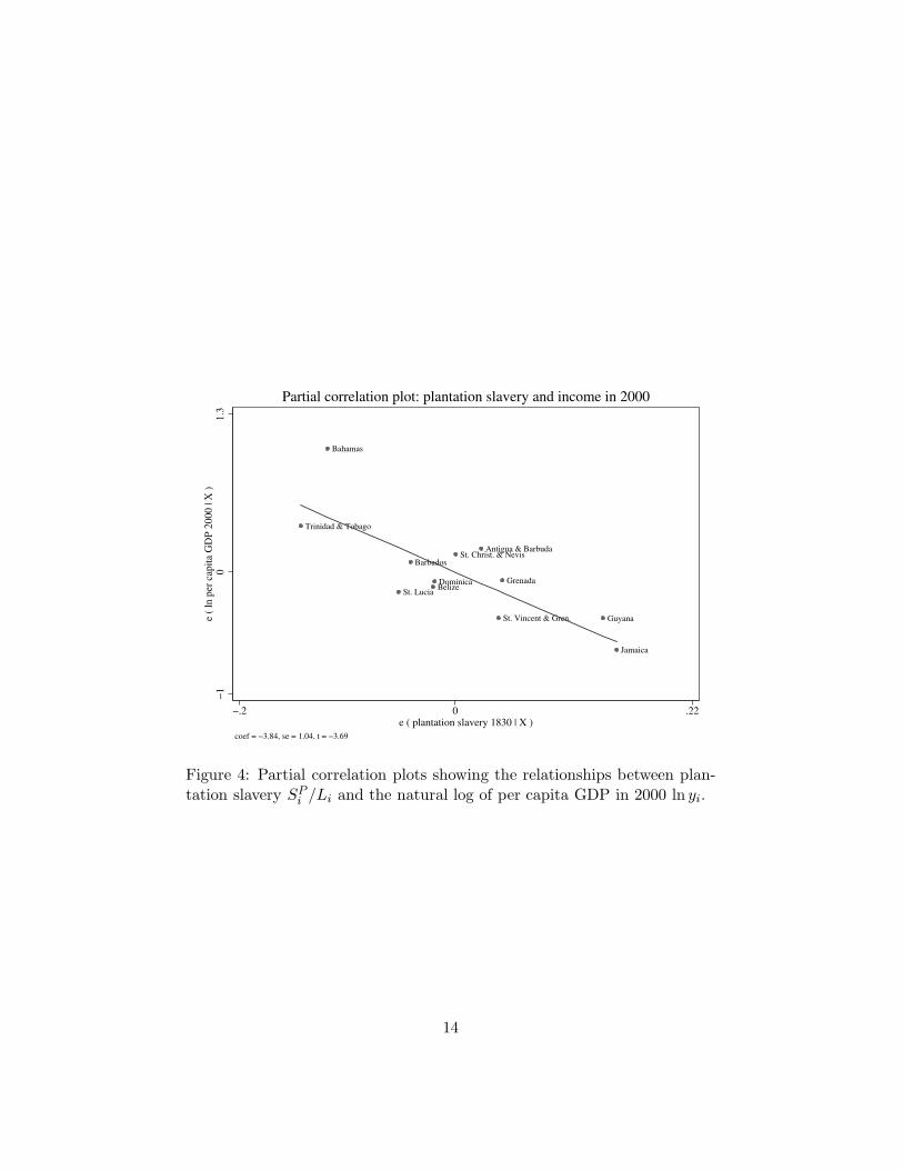
Estimates of (2) are reported in the third column of table 2. Both slaveryvariables enter with negative coefficients, and both coefficients are statisti-cally significant. These results confirm the previous negative relationshipbetween slave use and economic development. However, the relative magni-tudes of the coefficients do not support Engerman and Sokoloff’s focus onthe detrimental effects of large scale plantation agriculture. According tothe estimated magnitudes, it is not the use of slaves on large scale planta-tions that has the greatest negative impact on development, but the use ofnon-plantation slaves.

The partial correlation plots for the two slavery variables are shown infigures 3 and 4. From the plots it is apparent that neither relationship isbeing driven by a small number of outlying observations. Both relationshipsappear robust.

Next, I consider an alternative way of cutting the slavery data, andexamine whether the effect of slavery differs depending on the size of slaveholdings. Higman provides data on the number of slaves that are held onslave holdings with: (1) 10 slaves or less, (2) 11 to 50 slaves, (3) 51 to100 slaves, (4) 101 to 200 slaves, (5) 201 to 300 slaves, or (6) 301 slaves ormore.7 Because of the small number of observations available, I aggregatethe holdings into three categories: (1) small scale holdings of 10 slaves orless, (2) medium scale holdings with 11 to 200 slaves, and (3) large scaleholdings with 201 slaves or more. I then calculate of the proportion of thepopulation that are slaves held on small scale holdings SS

i /Li, medium scaleholdings SM

i /Li, and large scale holdings SLi /Li.

8

These measures provide an additional way of examining Engerman and

7Higman (1984, pp. 100–104) provides a detailed discussion of the difficulty of identify-ing a slave holding in the data. Slave holding are identified from each registration returnof the slave censuses. Slave owners that owned multiple plantations may have filled out adifferent form for each location. Also, if multiple owners owned slaves at one plantation,then these slaves may be identified as being in one slave holding.

8The conclusions reported here do not depend on the assumptions made in creatingthe categories. Alternatively, one could choose different cut-offs for the slave holdingcategories, or one could choose to create two categories rather than three, and the sameconclusions would be obtained.

11

Table 2: Slavery and income within the British West Indies.

Dependent variable: ln yi 1750 1830 1830 1830(1) (2) (3) (4)

Fraction of population that are:

Slaves, Si/Li −2.42∗∗∗−2.24∗∗

(.74) (.93)Non-plantation slaves, SNP

i /Li −6.55∗∗

(2.06)

Plantation slaves, SPi /Li −3.84∗∗∗

(1.04)Slaves on holdings with:

10 slaves or less, SSi /Li −20.92∗∗∗

(3.82)11 to 200 slaves, SM

i /Li −5.32∗∗∗

(.95)201 slaves or more, SL

i /Li −8.12∗∗∗

(1.30)

Population density, Li/Ai .24∗∗∗ .21∗∗∗ .20∗∗∗ .36∗∗∗

(.06) (.07) (.06) (.03)F-test of equality (p-value) .06 .00R2 .69 .55 .73 .96Number of observations 12 12 12 11

Notes: The table reports OLS estimates of equations (1), (2), and (3). The dependentvariables is the natural log of per capita GDP in 2000, ln yi. Coefficients are reportedwith standard errors in brackets. ∗∗∗, ∗∗, and ∗ indicate significance at the 1, 5, and10 percent levels. In column 1, all variables are measured in 1750, and in columns 2–4,all variables are measured in 1830. The null hypothesis of the reported F-test is theequality of the coefficients for the slavery variables.

12

Trinidad & Tobago

Bahamas

St. Lucia

DominicaBarbados

St. Christ. & NevisAntigua & Barbuda

St. Vincent & Gren.

Grenada

Belize

Guyana

Jamaica

−1

01

.3e

( ln

per

cap

ita

GD

P 2

00

0 |

X )

−.1 0 .12e ( non−plantation slavery 1830 | X )

coef = −6.55, se = 2.06, t = −3.17

Partial correlation plot: non−plantation slavery and income in 2000

Figure 3: Partial correlation plots showing the relationships between non-plantation slavery SNP

i /Li, and the natural log of per capita GDP in 2000ln yi.

13

Trinidad & Tobago

Bahamas

St. Lucia

Barbados

BelizeDominica

St. Christ. & NevisAntigua & Barbuda

St. Vincent & Gren.

Grenada

Guyana

Jamaica

−1

01

.3e

( ln

per

cap

ita

GD

P 2

00

0 |

X )

−.2 0 .22e ( plantation slavery 1830 | X )

coef = −3.84, se = 1.04, t = −3.69

Partial correlation plot: plantation slavery and income in 2000

Figure 4: Partial correlation plots showing the relationships between plan-tation slavery SP

i /Li and the natural log of per capita GDP in 2000 ln yi.

14

Table 3: Correlations between slave holding size and slave occupation acrosscountries within the British West Indies.

SSi /Li SM

i /Li SLi /Li

SPi /Li −.808 .881 .494

(.00) (.00) (.12)

SNPi /Li .649 −.843 −.232

(.03) (.00) (.49)

Notes: Pairwise correlation coefficient are reported with p-values in brackets. Each correlations is estimated across 11countries.

Sokoloff’s hypothesis that the detrimental impact of slavery arose becauseit was associated with economic inequality arising because of the existenceof large scale slave plantations. Across the countries in the sample, there isa strong positive relationship between the size of slave holdings and the useof slaves on plantations. This can be seen from table 3, which reports thecorrelation coefficients between the two measures of slave use disaggregatedby occupation and the three measures of slave use disaggregated by size ofslave holding. A clear pattern is apparent. The fraction of the populationthat are plantations slaves is negatively correlated with the fraction of thepopulation that are slaves on small scale holdings, and positively correlatedwith the fraction of the population that are slaves on medium and largescale holdings. These correlations confirm that the size of slave holdingsvariables provide an alternative indicator of the use of slaves on large scaleplantations. The relationship between slave holding size and the use of slavesis also shown in Higman (1984, pp. 104–106), where average slave holdingsize by slave use is provided for five of the colonies. The largest holdingstended to be on sugar plantations, followed by coffee, and then cotton. Thesmallest holdings were for slaves working in the livestock industry.

Allowing the effect of slavery to differ by the size of slave holdings, yieldsthe following estimating equation:

ln yi = α + βS SSi /Li + βM SM

i /Li + βL SLi /Li + γ Li/Ai + εi (3)

As before, this equation is simply a more flexible version of (1).

15

Trinidad & TobagoAntigua & Barbuda

St. Christ. & Nevis

St. Lucia

Grenada

St. Vincent & Gren.

GuyanaDominica

Barbados

Jamaica

Belize

−.5

0.6

e (

ln p

er c

apit

a G

DP

20

00

| X

)

−.03 0 .02e ( small scale slavery 1830 | X )

coef = −20.92, se = 3.82, t = −5.47

Partial correlation plot: small scale slavery and income in 2000

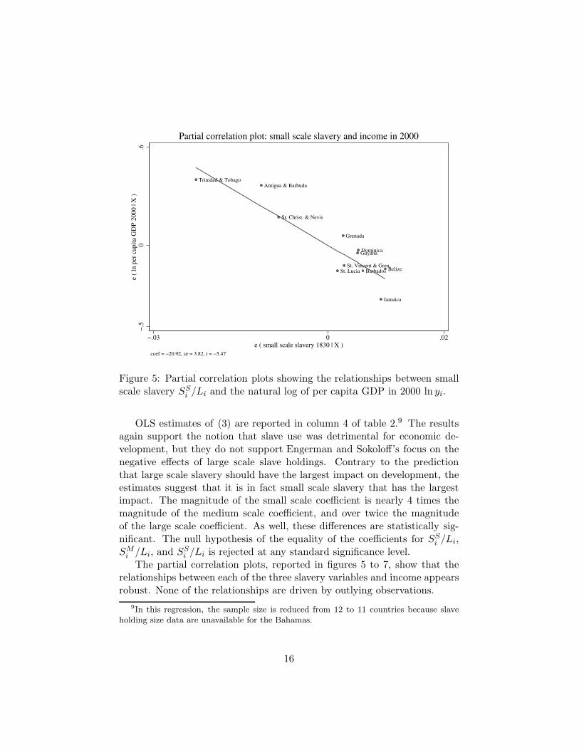
Figure 5: Partial correlation plots showing the relationships between smallscale slavery SS

i /Li and the natural log of per capita GDP in 2000 ln yi.

OLS estimates of (3) are reported in column 4 of table 2.9 The resultsagain support the notion that slave use was detrimental for economic de-velopment, but they do not support Engerman and Sokoloff’s focus on thenegative effects of large scale slave holdings. Contrary to the predictionthat large scale slavery should have the largest impact on development, theestimates suggest that it is in fact small scale slavery that has the largestimpact. The magnitude of the small scale coefficient is nearly 4 times themagnitude of the medium scale coefficient, and over twice the magnitudeof the large scale coefficient. As well, these differences are statistically sig-nificant. The null hypothesis of the equality of the coefficients for SS

i /Li,SM

i /Li, and SSi /Li is rejected at any standard significance level.

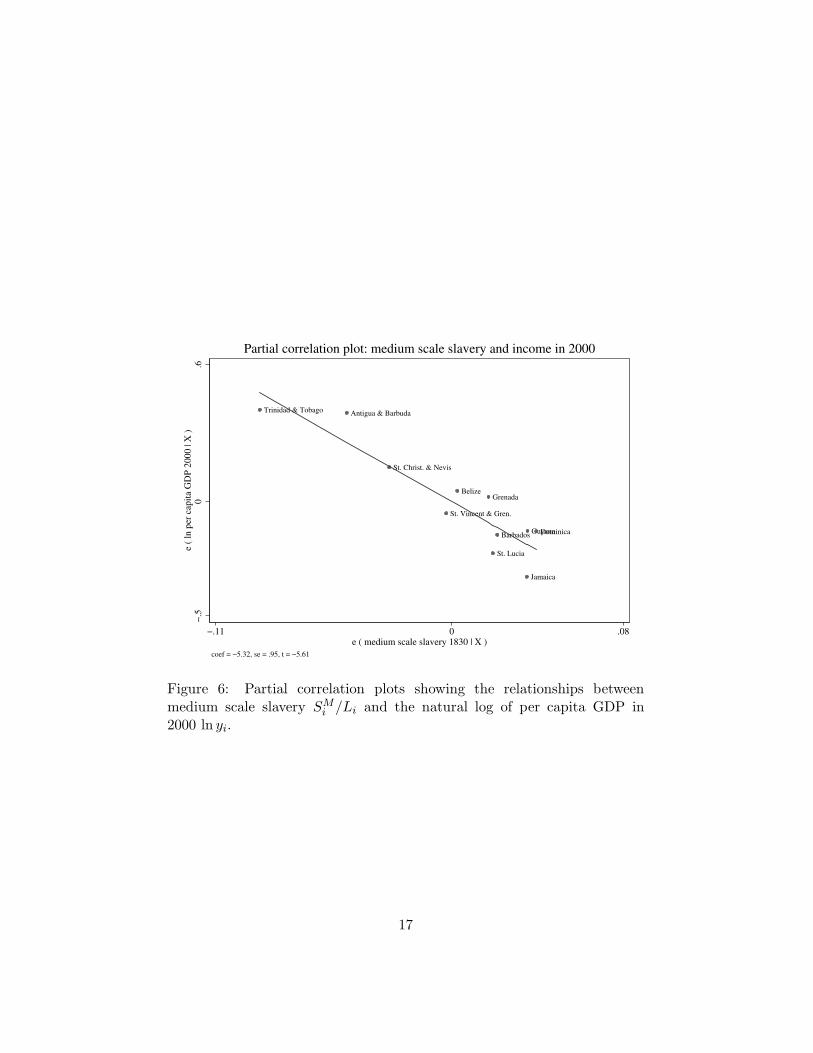
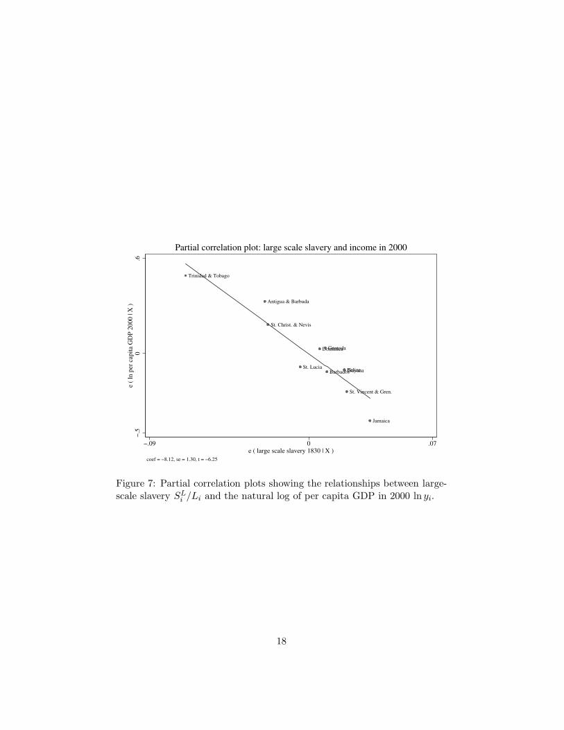
The partial correlation plots, reported in figures 5 to 7, show that therelationships between each of the three slavery variables and income appearsrobust. None of the relationships are driven by outlying observations.

9In this regression, the sample size is reduced from 12 to 11 countries because slaveholding size data are unavailable for the Bahamas.

16

Trinidad & Tobago Antigua & Barbuda

St. Christ. & Nevis

St. Vincent & Gren.

BelizeGrenada

St. Lucia

Barbados

Jamaica

GuyanaDominica

−.5

0.6

e (

ln p

er c

apit

a G

DP

20

00

| X

)

−.11 0 .08e ( medium scale slavery 1830 | X )

coef = −5.32, se = .95, t = −5.61

Partial correlation plot: medium scale slavery and income in 2000

Figure 6: Partial correlation plots showing the relationships betweenmedium scale slavery SM

i /Li and the natural log of per capita GDP in2000 ln yi.

17

Trinidad & Tobago

Antigua & Barbuda

St. Christ. & Nevis

St. Lucia

DominicaGrenada

BarbadosBelizeGuyana

St. Vincent & Gren.

Jamaica

−.5

0.6

e (

ln p

er c

apit

a G

DP

20

00

| X

)

−.09 0 .07e ( large scale slavery 1830 | X )

coef = −8.12, se = 1.30, t = −6.25

Partial correlation plot: large scale slavery and income in 2000

Figure 7: Partial correlation plots showing the relationships between large-scale slavery SL

i /Li and the natural log of per capita GDP in 2000 ln yi.

18

Overall, these results confirm the previous findings in section 2.1. Look-ing within the British West Indies, the data provide support for Sokoloff andEngerman’s hypothesis that slavery adversely affected subsequent economicdevelopment. However, they do not support their emphasis on the adverseeffects of large scale plantation slavery. According to the estimates, all formsof slavery appear similarly detrimental for economic development. There isno evidence that large scale plantation slavery was more detrimental thanother forms of slavery.

2.3 Looking within the United States

I now turn to a different source of evidence, and compare the relative de-velopment of counties and states within the U.S. Using information on thenumber of slaves and free persons in each county and state in each decadebetween 1790 and 1860, I again examine Engerman and Sokoloff’s assertionthat domestic slavery was detrimental for subsequent economic development.Population data for slaves and free persons are taken from the U.S. Decen-nial Censuses, while income data are from the BEA’s Regional EconomicAccounts.

The cross-state relationship between the proportion of the population inslavery in 1860, the year for which data are available for the largest numberof states, and the natural log of per capita income in 2000 is shown in figure8. The figure shows a clear negative relationship between slave use andsubsequent economic performance.

I explore this relationship further in table 4. Each column of the tablereports the estimated relationship between slavery in each decade between1790 and 1860 and log per capita income in 2000, controlling for initial pop-ulation density measured in the same year as slavery. The top panel of thetable reports the relationship between the proportion of the population inslavery and per capita income across U.S. states. The number of observa-tions begins at 17 in 1790 (the first column) and increases each decade to37 in 1860 (the last column). The reason that the 1790 estimates include17 states when only 13 states had joined the Union is that census data arealso available for West Virginia, Kentucky, Maine, and Vermont. In 1790West Virginia and Kentucky were part of Virginia, while Maine was a partof Massachusetts. Therefore, data are available for these three areas thatlater became independent states. As well, data are also available for theVermont Republic which joined the Union a year later in 1791, becomingthe state of Vermont.10

10Similarly, in 1800 there are 18 observations even though only 16 states had joined the

19

Alabama

Arkansas

California

Connecticut

Delaware

FloridaGeorgia

Illinois

IndianaIowa

Kansas

Kentucky

Louisiana

Maine

Maryland

Massachusetts

Michigan

Minnesota

Mississippi

MissouriNebraska

Nevada

New Hampshire

New Jersey

New York

North Carolina

OhioOregon

PennsylvaniaRhode Island

South Carolina

Tennessee

TexasVermont

Virginia

West Virginia

Wisconsin

9.9

10

.7ln

in

com

e p

er c

apit

a, 2

00

0

0 .32 .64slaves / total population, 1860

beta coef = −.52, t−stat = −3.63, N = 37

Relationship between slavery in 1860 and income in 2000

Figure 8: Bivariate plot showing the relationship between the proportionof the population in slavery 1860 Si/Li and the natural log of per capitaincome in 2000 ln yi.

20

All of the estimated coefficients for the fraction of population in slaverySi/Li are negative. For the three decades prior to 1820 the coefficients arestatistically insignificant, while for the five decades after 1810 the coefficientsare statistically significant. The insignificance of the results for the first threedecades is because three important slave states (Louisiana, Mississippi, andAlabama) did not join the Union until the decade after 1810. This can alsobe seen in figure 8. If one omits these three states, the negative relationshipis weakened substantially.

The magnitudes of the estimated coefficients are large. When controllingfor initial population density, the standardized beta coefficients range from−.09, for 1790, to −.41, for 1860. According to the 1860 estimates, if in1860 South Carolina had no slavery, rather than 57% of its population inslavery, then its average per capita income in 2000 would have been $29,400rather than $24,300. This is an increase in income of over 20%.

The second panel of table 4 reports the same estimates looking acrosscounties rather than states. As in the state level regressions, the coeffi-cient estimates for Si/Li are negative. To be as conservative as possible,I allow for non-independence of counties within a state, and report stan-dard errors clustered at the state level. This tends to at least double thereported standard errors. The coefficient estimates are negative and statis-tically significant for every year except 1810. Again, the coefficients are alsoeconomically large. The beta coefficients range from −.13 to −.23.

Union by this time. This is because of West Virginia and Maine.

21

Table 4: Slavery and income across counties and states within the U.S.

Dependent variable: ln yi 1790 1800 1810 1820 1830 1840 1850 1860

State level regressions

Fraction slaves, Si/Li −.13 −.10 −.11 −.28∗−.29∗∗

−.27∗∗−.34∗∗

−.33∗∗∗

(.24) (.23) (.20) (.15) (.14) (.13) (.13) (.11)Population density, Li/Ai .52∗∗ .57∗∗∗ .52∗∗∗ .46∗∗∗ .40∗∗∗ .33∗∗∗ .19∗∗ .16∗∗∗

(.20) (.19) (.17) (.13) (.11) (.10) (.07) (.05)R2 .38 .43 .44 .53 .53 .48 .42 .43Number of observations 17 18 19 25 27 30 33 37

County level regressions

Fraction slaves, Si/Li −.28∗∗−.21∗

−.15 −.17∗−.19∗∗

−.24∗∗∗−.23∗∗∗

−.22∗∗∗

(.11) (.12) (.10) (.10) (.09) (.08) (.08) (.07)Population density, Li/Ai .09∗∗∗ .06∗∗∗ .04∗∗∗ .03∗∗∗ .02∗∗ .01∗∗∗ .007∗∗∗ .004∗∗∗

(.01) (.01) (.007) (.006) (.003) (.002) (.001) (.001)R2 .17 .13 .10 .09 .09 .09 .08 .07Number of observations 283 400 521 739 964 1,273 1,588 2,014

Notes: The dependent variables is the natural log of per capita income in 2000, ln yi. Coefficients are reported withstandard errors in brackets. For the county level estimates the standard errors are clustered at the state level. ∗∗∗,∗∗, and ∗ indicate significance at the 1, 5, and 10 percent levels. Population density Li/Ai is measured in the sameyear as slavery.

22

The estimated relationship between slave use and subsequent economicperformance reported in table 4 are consistent with the recent findings ofMitchener and McLean (2003) and Lagerlof (2005). Mitchener and McLean(2003) estimate the relationship between slave use and subsequent laborproductivity across U.S. states, and find a significant negative relationshipbetween the fraction of the population in slavery in 1860 and average laborproductivity in the decades after this date. Lagerlof (2005), looking acrossU.S. counties, also documents a negative relationship between past slave use,measured in 1850, and subsequent per capita income measured in 1994.

The 1860 Census also reports the total number of slave holders that holdthe following number of slaves: 1, 2, 3, 4, 5, 6, 7, 8, 9, 10–14, 15–19, 20–29,30–39, 40–49, 50–69, 70–99, 100–199, 200–299, 300–499, 500–999, and 1,000and over. Because the census only reports information on the size holdingof each slave holder and not of each slave (as in the Higman data), I canonly calculate the number of slaves held in each size holding when the exactnumber of slaves per holder is given, which is only for holdings with lessthan 10 slaves. Therefore, although I can separate small scale holdings (9slaves or less) from medium or large scale holdings, I am unable to separateslaves held on medium scale holdings (10 to 199 slaves) from those held onlarge holdings (200 slaves or more).11

Using the Census data, I construct two measures of slavery: the propor-tion of the population that are slaves held on small scale holdings SS

i /Li,and the proportion of the population that are slaves held on medium orlarge scale holdings SML

i /Li. As before, I allow the two types of slavery toaffect economic development differently:

ln yi = α + βS SSi /Li + βML SML

i /Li + γ Li/Ai + εi (4)

The subscript i indexes either counties or states, and as before ln yi andLi/Ai denote log income in 2000 and initial population density.

Table 5 reports the estimates of (4). The first column reports estimateswhere a state is the unit of observation. The coefficients for SS

i /Li andSML

i /Li are both negative, but neither is statistically significant. Their in-significance appears to be the result of multi-collinearity. The correlationbetween SS

i /Li and SMLi /Li is .87. Although neither coefficient is individu-

ally significant, jointly the two coefficients are significant. An F-test of theirjoint significance is able to reject the null hypothesis that both coefficients

11Note that because of these same data limitations, the definition of small scale is slightlydifferent than in section 2.2. Here the definition of small scale is 9 slaves or less, while thedefinition in section 2.2 was 10 slaves or less.

23

are jointly equal to zero at the 2 percent level. This can also be seen fromthe R2, which increases from .28 to .43, when the two variables are includedin the estimating equation.

Turning to the point estimates, I find that contrary to Engerman andSokoloff’s hypothesis, there is no evidence that large scale slavery is moredetrimental for development than small scale slavery. Although these pointestimates do not support Engerman and Sokoloff’s focus on large scale plan-tation slavery, it is possible that the data are not sufficiently rich to identifythe more harmful effects of medium/large scale slavery relative to small scaleslavery. For this reason, I also examine county level data, which providesfiner variation that can help to better identify the differential effects of slav-ery. At the county level the collinearity between SS

i /Li and SMLi /Li is .65,

which is lower than the correlation at the state level.Column 2 reports county level estimates. Again, the results do not

provide a clear indication that large scale slavery had a worse impact oneconomic development relative to other forms of slavery. The estimatedcoefficients for both SS

i /Li and SMLi /Li are negative. Looking at the mag-

nitudes, small scale slavery is estimated to be slightly worse for economicdevelopment than large scale slavery, although the difference between thetwo coefficients is not statistically different from zero. Looking at the statis-tical significance of the coefficients, it is only medium/large scale slavery thatis statistically different from zero. Therefore, the results appear mixed anddiffer depending on whether one considers the magnitudes of the estimatedcoefficients or their statistical significance. As before, the evidence does notclearly indicate that large scale plantation slavery was more detrimental foreconomic development than other forms of slavery.

Overall, the results of this section show that, either looking across NewWorld economies, or across counties and states within the U.S., there is anegative relationship between past slave use and current economic develop-ment. However, the results do not provide support for the view that largescale plantation agriculture was particularly detrimental. All forms of slav-ery – smaller scale non-plantation forms of slavery and large scale plantationslavery – appear to have had similarly detrimental effects on economic de-velopment.

24

Table 5: Slavery and income within the United States.

State level County levelDependent variable: ln yi regressions regressions

(1) (2)

Fraction of the population that are slaves:

on holdings with 9 slaves or less, SSi /Li −.41 −.24

(.99) (.25)on holdings with 10 slaves or more, SML

i /Li −.31 −.22∗∗∗

(.26) (.06)

Population density, Li/Ai .16∗∗∗ .004∗∗∗

(.05) (.0006)

F-test of equality (p-value) .93 .94R2 .43 .07Number of observations 37 2,014

Notes: The dependent variables is the natural log of per capita income in 2000, ln yi.Coefficients are reported with standard errors in brackets. ∗∗∗, ∗∗, and ∗ indicatesignificance at the 1, 5, and 10 percent levels. For the county level estimates thestandard errors are clustered at the state level. In column 1 the unit of observationis a U.S. state and in column 2 the unit of observations is a U.S. county. The slaveryand populations density variables are measured in 1860.

25

3 Testing Specific Channels of Causality

I now turn to the specific channels of causality underlying the negative rela-tionship between slavery and economic development. Recall, that Engermanand Sokoloff’s argument is that plantation slavery resulted in increased eco-nomic inequality, which resulted in subsequent economic underdevelopment.This chain of causality is illustrated in diagram 1.

Plantation=⇒

Economic=⇒

EconomicSlavery Inequality Underdevelopment

Diagram 1: Testing the channels of causality in Engerman and Sokoloff’shypothesis.

In the previous section, I simultaneously examined both parts of theirargument, testing for a reduced form relationship between slavery and eco-nomic development. In this section, using data on the distribution of landholdings from the 1860 U.S. Census, I examine Engerman and Sokoloff’s ar-gument that slavery was detrimental because of its effect on initial economicinequality. That is, I examine separately both hypothesized relationshipsfrom diagram 1: (i) that plantation slavery resulted in increased economicinequality, and (ii) that inequality resulted in economic underdevelopment.The first hypothesis is examined in the section 3.1, and the second is exam-ined in section 3.2.

3.1 Testing Relationship 1: Plantation Slavery ⇒ Economic

Inequality

The 1860 U.S. Census provides data on the number of farms, in each countyand state, that are in each of the following seven size categories: (1) 9 acresor less, (2) 10 to 19 acres, (3) 20 to 49 acres, (4) 50 to 99 acres, (5) 100to 499 acres, (6) 500 to 999 acres, and (7) 1,000 acres or more. I use thisinformation to construct, for each county and state, the Gini coefficient ofland inequality in 1860. Full details of the construction are provided in theappendix.

I examine whether the data support Engerman and Sokoloff’s view thatslavery resulted in increased economic inequality by first considering the un-conditional relationship between the proportion of the population in slavery

26

Alabama

Arkansas

California

Connecticut

Delaware

Florida

Georgia

Illinois

Indiana

Iowa

Kansas

Kentucky

Louisiana

Maine

Maryland

Massachusetts

Michigan

Minnesota

Mississippi

Missouri

Nebraska

Nevada

New Hampshire

New Jersey

New York

North Carolina

Ohio

Oregon

Pennsylvania

Rhode IslandSouth Carolina

Tennessee

Texas

Vermont

Virginia

West Virginia

Wisconsin

.37

.57

Gin

i co

effi

cien

t o

f la

nd

in

equ

alit

y,

18

60

0 .35 .65slaves / total population, 1860

beta coef = .53, t−stat = 3.74, N = 37

Relationship between slavery in 1860 and land inequality in 1860

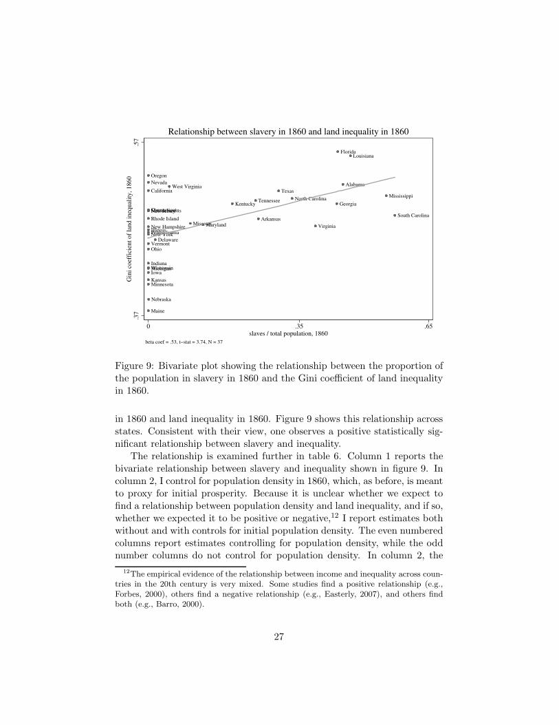
Figure 9: Bivariate plot showing the relationship between the proportion ofthe population in slavery in 1860 and the Gini coefficient of land inequalityin 1860.

in 1860 and land inequality in 1860. Figure 9 shows this relationship acrossstates. Consistent with their view, one observes a positive statistically sig-nificant relationship between slavery and inequality.

The relationship is examined further in table 6. Column 1 reports thebivariate relationship between slavery and inequality shown in figure 9. Incolumn 2, I control for population density in 1860, which, as before, is meantto proxy for initial prosperity. Because it is unclear whether we expect tofind a relationship between population density and land inequality, and if so,whether we expected it to be positive or negative,12 I report estimates bothwithout and with controls for initial population density. The even numberedcolumns report estimates controlling for population density, while the oddnumber columns do not control for population density. In column 2, the

12The empirical evidence of the relationship between income and inequality across coun-tries in the 20th century is very mixed. Some studies find a positive relationship (e.g.,Forbes, 2000), others find a negative relationship (e.g., Easterly, 2007), and others findboth (e.g., Barro, 2000).

27

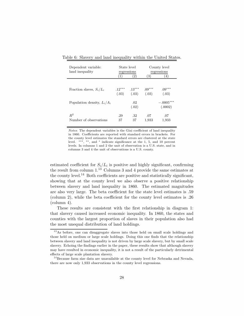
Table 6: Slavery and land inequality within the United States.

Dependent variable: State level County levelland inequality regressions regressions

(1) (2) (3) (4)

Fraction slaves, Si/Li .12∗∗∗ .13∗∗∗ .09∗∗∗ .09∗∗∗

(.03) (.03) (.03) (.03)

Population density, Li/Ai .02 −.0005∗∗∗

(.02) (.0002)

R2 .29 .32 .07 .07Number of observations 37 37 1,933 1,933

Notes: The dependent variables is the Gini coefficient of land inequalityin 1860. Coefficients are reported with standard errors in brackets. Forthe county level estimates the standard errors are clustered at the statelevel. ∗∗∗, ∗∗, and ∗ indicate significance at the 1, 5, and 10 percentlevels. In columns 1 and 2 the unit of observation is a U.S. state, and incolumns 3 and 4 the unit of observations is a U.S. county.

estimated coefficient for Si/Li is positive and highly significant, confirmingthe result from column 1.13 Columns 3 and 4 provide the same estimates atthe county level.14 Both coefficients are positive and statistically significant,showing that at the county level we also observe a positive relationshipbetween slavery and land inequality in 1860. The estimated magnitudesare also very large. The beta coefficient for the state level estimates is .59(column 2), while the beta coefficient for the county level estimates is .26(column 4).

These results are consistent with the first relationship in diagram 1:that slavery caused increased economic inequality. In 1860, the states andcounties with the largest proportion of slaves in their population also hadthe most unequal distribution of land holdings.

13As before, one can disaggregate slaves into those held on small scale holdings andthose held on medium or large scale holdings. Doing this one finds that the relationshipbetween slavery and land inequality is not driven by large scale slavery, but by small scaleslavery. Echoing the findings earlier in the paper, these results show that although slaverymay have resulted in economic inequality, it is not a result of the particularly detrimentaleffects of large scale plantation slavery.

14Because farm size data are unavailable at the county level for Nebraska and Nevada,there are now only 1,933 observations in the county level regressions.

28

Alabama

Arkansas

CaliforniaConnecticut

Delaware

Florida

Georgia

Illinois

Indiana

Iowa

Kansas

Kentucky

Louisiana

Maine Maryland

Massachusetts

Michigan

Minnesota

Mississippi

Missouri

Nebraska

Nevada

New Hampshire

New Jersey

New York

North Carolina

OhioOregon

Pennsylvania

Rhode IslandSouth Carolina

Tennessee

Texas

Vermont

Virginia

West Virginia

Wisconsin

.41

.5G

ini

coef

fici

ent

of

inco

me

ineq

ual

ity

, 2

00

0

.38 .58Gini coefficient of land inequality, 1860

beta coef = .65, t−stat = 5.13, N = 37

Relationship between land inequality in 1860 and income inequality in 2000

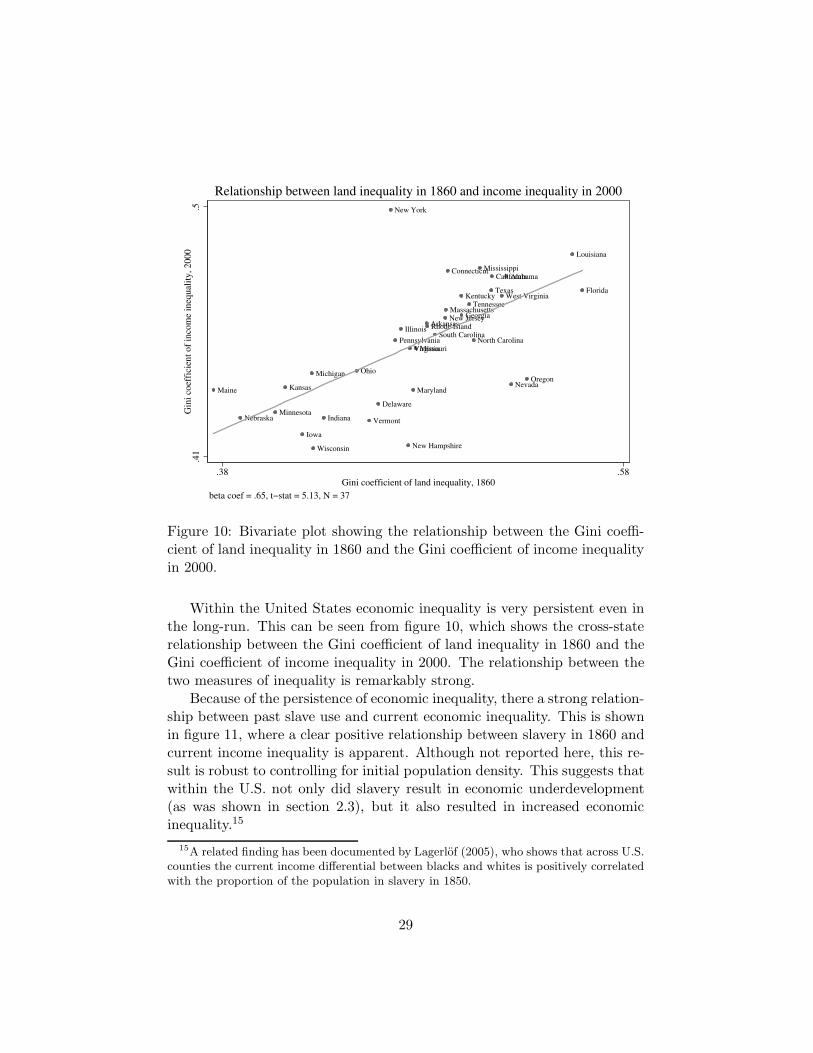
Figure 10: Bivariate plot showing the relationship between the Gini coeffi-cient of land inequality in 1860 and the Gini coefficient of income inequalityin 2000.

Within the United States economic inequality is very persistent even inthe long-run. This can be seen from figure 10, which shows the cross-staterelationship between the Gini coefficient of land inequality in 1860 and theGini coefficient of income inequality in 2000. The relationship between thetwo measures of inequality is remarkably strong.

Because of the persistence of economic inequality, there a strong relation-ship between past slave use and current economic inequality. This is shownin figure 11, where a clear positive relationship between slavery in 1860 andcurrent income inequality is apparent. Although not reported here, this re-sult is robust to controlling for initial population density. This suggests thatwithin the U.S. not only did slavery result in economic underdevelopment(as was shown in section 2.3), but it also resulted in increased economicinequality.15

15A related finding has been documented by Lagerlof (2005), who shows that across U.S.counties the current income differential between blacks and whites is positively correlatedwith the proportion of the population in slavery in 1850.

29

Alabama

Arkansas

CaliforniaConnecticut

Delaware

Florida

Georgia

Illinois

Indiana

Iowa

Kansas

Kentucky

Louisiana

Maine Maryland

Massachusetts

Michigan

Minnesota

Mississippi

Missouri

Nebraska

Nevada

New Hampshire

New Jersey

New York

North Carolina

OhioOregon

Pennsylvania

Rhode IslandSouth Carolina

Tennessee

Texas

Vermont

Virginia

West Virginia

Wisconsin

.41

.5G

ini

coef

fici

ent

of

inco

me

ineq

ual

ity

, 2

00

0

0 .32 .65slaves / total population, 1860

beta coef = .47, t−stat = 3.15, N = 37

Relationship between slavery in 1860 and income inequality in 2000

Figure 11: Bivariate plot showing the relationship between the proportion ofthe population in slavery in 1860 and the Gini coefficient of income inequalityin 2000.

30

3.2 Testing Relationship 2: Economic Inequality ⇒ Eco-

nomic Development

The second part of Engerman and Sokoloff’s hypothesis is that the economicinequality that arose because of slavery resulted in economic underdevelop-ment. They argue that inequality resulted in domestic institutions thatadvantaged the elites, rather than providing the foundation necessary forsustained economic growth. In columns 1 and 4 of table 7, I empiricallytest for a relationship between initial economic inequality and subsequenteconomic development. The columns report the estimated relationship be-tween the Gini coefficient of land inequality in 1860 and income in 2000,controlling for initial population density. Column 1 reports estimates at thestate level, while column 4 reports estimates at the county level. In bothspecifications, the estimated coefficient for land inequality is negative, butstatistically insignificant. Although the sign of the coefficient is consistentwith inequality adversely affecting development, its insignificance shows thatstatistically its estimated effect is not different from zero.

There is also a second testable prediction that follows from Sokoloff andEngerman’s argument. According to their hypothesis, the estimated rela-tionship between slavery and economic development (which was reported intable 4) should be accounted for by the relationship between initial inequal-ity and economic development. The remaining columns in table 7 test thisprediction of their theory. Columns 2 and 5, revisit the estimated relation-ship between slavery and economic development previously reported in table4. Column 2 simply reproduces the 1860 state level estimates, and column5 re-estimates the county-level regressions, using a slightly smaller sampleof counties for which land inequality data are also available. Because farmsize data are missing for the counties of Nebraska and Nevada, they are notincluded in the sample. This results in a reduction in the sample size from2,014 to 1,933 counties. As shown, one still finds a negative relationshipbetween slavery and income among this smaller sample of counties.

Columns 3 and 6 test whether the estimated relationships between slav-ery and income in columns 2 and 5 can be accounted for by the relationshipbetween land inequality and income. This is done by including both theGini coefficient of land inequality and the fraction of slaves in the popula-tion as explanatory variables in the estimating equation. If slavery affectsincome only through its effect on initial economic inequality, then controllingfor inequality should significantly reduce the estimated relationship betweenslavery and income. The results show that this is not the case. At both thestate and the county levels, including the land inequality measure actually

31

increases the magnitude of the estimated coefficient for Si/Li, rather thandecreasing it. At the state level, the estimated effect increases from −.33 to−.39, and at the county level, the effect increases from −.23 to −.24. Theresults, therefore, do not support Engerman and Sokoloff’s argument thatslavery adversely affecte economic development because it resulted in initialinequality.

The results in table 7 show clearly that land inequality in 1860 is un-correlated with income in 2000. These results are particularly interestinggiven that others have found evidence that early land inequality had ad-verse effects on outcomes measured in the early 1900s. Ramcharan (2006)finds a negative relationship between early land inequality and per capitaeducation expenditures in 1930, and Acemoglu et al. (2007) document anegative relationship between land inequality in 1860 and school enrollmentin 1950. The estimates from table 7 suggest that the effects documentedby Ramcharan (2006) and Acemoglu et al. (2007) died out by the end ofthe 20th century. This is not surprising given that beginning in the 1940s,average incomes in the Southern states began to catch-up to the Northernstates (Wright, 1987), and given the fact that the black-white education gapand the black-white wage gap have both decreased significantly since 1940(Smith and Welch, 1989).

32

Table 7: Slavery, land inequality, and income within the United States.

Dependent variable: ln yi State level regressions County level regressions

(1) (2) (3) (4) (5) (6)

Gini coefficient of land inequality −.46 .45 −.11 .07(.51) (.55) (.11) (.11)

Fraction slaves, Si/Li −.33∗∗∗−.39∗∗∗

−.23∗∗∗−.24∗∗∗

(.11) (.13) (.07) (.07)Population density: Li/Ai .21∗∗∗ .16∗∗∗ .15∗∗∗ .004∗∗∗ .004∗∗∗ .004∗∗∗

(.06) (.05) (.05) (.0006) (.0006) (.0006)R2 .30 .43 .45 .03 .08 .08Number of observations 37 37 37 1,933 1,933 1,933

Notes: The dependent variables is the natural log of per capita income in 2000, ln yi. Coefficients arereported with standard errors in brackets. For the county level estimates the standard errors are clusteredat the state level. ∗∗∗, ∗∗, and ∗ indicate significance at the 1, 5, and 10 percent levels. In columns 1–3 theunit of observation is a U.S. state, and in columns 4–6 the unit of observations is a U.S. county.

33

The results of section 3 are best summarized by returning to diagram 1.There is evidence of the first relationship in the diagram. Slavery in 1860is associated with greater land inequality in the same year. This was shownin table 6. Further, as a result of the persistence of economic inequality,there is also a strong positive relationship between slavery and current in-come inequality. However, I do not find evidence for the second relationshipin diagram 1. The results of table 7 show that land inequality in 1860 isnot correlated with income in 2000. They also show that the positive re-lationship between slavery and inequality is unable to explain the negativerelationship between slavery and economic development. Instead, the datasuggest that slavery had two distinct impacts. First, slavery resulted inlower long-term economic growth, and second, slavery resulted in greaterinitial inequality, which has persisted until today. These two effects appearto be unrelated. Contrary to Engerman and Sokoloff’s hypothesis, slaverywas not detrimental for economic development because it increased initialeconomic inequality.

Although these results take us a step towards better understanding thelong-term impacts of slavery in the Americas, an important question re-mains. If the relationship between past slave use and current income is notthrough the channel hypothesized by Engerman and Sokoloff, then what ex-plains the relationship? One possibility, which is highlighted by Acemogluet al.’s (2007) chapter in this book, is that what may have been important forlong-term economic development was political inequality, not economic in-equality. The authors, looking within Cundinamarca Colombia, show thateconomic and political inequality are not always strongly correlated, andthat they can diverge in significant ways. When examining the relationshipbetween inequality and economic development, they find that one reachesvery different conclusions depending on whether one looks at economic in-equality or political inequality. It is possible that the results reported herewould be very different if political inequality, rather than economic inequal-ity, was examined.

A second possibility follows from Wright (2006), who argues that slav-ery’s long-term effects are best understood by comparing its property rightsinstitutions to those that arise from a production system based on free labor.Because slavery provided slave owners with property rights over labor, whichallowed them to relocate labor as necessary, the slave states did not havea strong incentive to provide the public goods and institutions necessaryto attract migrants (Wright, 2006, pp. 70–77). This channel is similar toEngerman and Sokoloff’s, but is different in a subtle yet important way. Itis not economic inequality that caused the subsequent development of poor

34

institutions. Rather, it was slavery itself. Through the purchase and sale ofslaves, involuntary migration could substitute for voluntary migration, andtherefore, the growth promoting domestic institutions needed to attract freelabor were not developed.

4 Conclusions

This chapter has examined the core predictions that arise from a series ofinfluential papers written by Stanley Engerman and Kenneth Sokoloff (e.g.,Engerman and Sokoloff, 1997, 2002, 2006; Sokoloff and Engerman, 2000).Examining the relationship between past slave use and current economicperformance, I find evidence consistent with their general hypothesis thatslavery was detrimental for economic development. Looking either acrosscountries within the Americas, or across states and counties within the U.S.,one finds a strong significant negative relationship between past slave useand current income. However, contrary to the focus of their argument, thedata do not show that large scale plantation slavery was more harmful forgrowth than other forms of slavery. Instead, the evidence suggests that allforms of slavery were equally detrimental.

Turning to their hypothesized channels of causality, I examined whetherthe relationship between slavery and income can be explained by slavery’seffect on initial economic inequality. Looking within the U.S., I found that,consistent with their hypothesis, slave use in 1860 is positively correlatedwith land inequality in the same year. Because of the persistence of inequal-ity overtime, past slave use is also positively correlated with current incomeinequality. Thus, the data suggest that slavery had a long-term effect oninequality as well as income. However, after examining the relationship be-tween slave use, initial inequality, and current income, I found that slavery’seffect on initial economic inequality is unable to account for any of the es-timated relationship between slavery and economic development. Contraryto their hypothesis, slavery’s adverse effect on economic development doesnot appear to be because of its effect on initial economic inequality.

A Data Appendix

Data on country level per capita GDP in 2000 are from World Bank (2006).For countries with missing income data, when possible converted incomedata from the Penn World Tables or Maddison (2003) were used. For bothseries, data are measured in PPP adjusted dollars. State and county level per

35

capita income in 2000 are from the BEA’s Regional Economic Accounts. Thecounty level data are from Table CA1-3 located at www.bea.gov/regional/reis/,and the state level data are from Table SA1-3 at www.bea.gov/regional/spi/.

Population density is measured in hundreds of persons per square kilome-ter in the cross-country regressions, and hundreds of persons per square milein the county and state level regressions. Country level land area data arefrom Harvard’s Center for International Development’s Geography Databaselocated at www.ksg.harvard.edu/CID/ciddata/Geog/physfact rev.dta. Landarea for U.S. states and counties are from U.S. Bureau of the Census (2006).

The country level slave and free populations data used in section 2.1 arefrom a variety of sources. All data are from 1750 or the closest available year.Figures for Barbados, Saint Christopher and Nevis, Antigua and Barbuda,Jamaica, Cuba, Dominica, Saint Lucia, Saint Vincent and the Grenadines,Trinidad and Tobago, Grenada, Guyana, Belize, Bahamas, Haiti, Suriname,Netherlands Antilles, and the Dominican Republic are from Engerman andHigman (1997). All figures are for 1750. Data for Canada are from the1784 Census of Canada. Data for the United States are for 1774 and arefrom Jones (1980). Brazilian data are for 1798 and are taken from Simonsen(1978, pp. 54–57). Chilean data are from 1777 and are from Sater (1974).The figures for Colombia are for 1778 and are from McFarlane (1993). Datafor Ecuador are for 1800 and are from Restrepo (1827, p. 14). Mexican dataare for 1742 and are from Aguirre Beltran (1940, pp. 220–223). Peruviandata are for 1795 and are from Rugendas (1940). Data from Paraguay arefor 1782 and are from Acevedo (1996, pp. 200–206). Venezuelan data are for1800 and are taken from Figueroa (1983, p. 58). Data for Uruguay are forthe city of Montevideo in 1800, and are taken from Williams (1987). Datafor Argentina are for the city of Buenos Aires in 1810, and are from RoutJr. (1976, pp. 91, 95) and Johnson et al. (1980).

Slave and free populations data for counties and states within the U.S.are from the 1790 to 1860 Decennial Censuses of the United States. The datahave been digitized and can be accessed at: http://fisher.lib.virginia.edu/collections/stats/histcensus/. The data on the size of slave holdings, andthe size of farms in 1860 are also from this source.

The Gini coefficient of income inequality for each state in 2000 is fromthe U.S. Census Bureau. I approximate income inequality in 2000 usinginequality in 1999, which is the closest year for which the inequality mea-sures are available. The data were accessed from Table S4 available at:www.census.gov/hhes/www/income/histinc/state/state4.html

The Gini coefficient of land inequality is calculated using informationabout the size of each farm in the 1860 Census. The number of farms in

36

each county is available for the following farm sizes: (1) 9 acres or less, (2)10 to 19 acres, (3) 20 to 49 acres, (4) 50 to 99 acres, (5) 100 to 499 acres, (6)500 to 999 acres, and (7) 1,000 acres or more. Because for each category Ido not know the mean farm size, I use the median size of the category. Forthe category 1,000 acres or more, I use 1,000 acres. The Gini coefficients arecalculated using the Stata program ineqdec0 written by Stephen P. Jenkins.The formula for calculating the Gini coefficient is:

1 + (1/n) −2∑n

i=1(n − i + 1)ai

n∑n

i=1 ai

where n is the number of farms, ai is farm size, and i denotes the rank,where farms are ranked in ascending order of ai.

References

Acemoglu, Daron, Marıa Angelica Bautista, Pablo Querubın, and James A.Robinson, “Economic and Political Inequality in Development: The Caseof Cundinamarca, Colombia,” (2007), mimeo, M.I.T.

Acemoglu, Daron, Simon Johnson, and James A. Robinson, “Reversal ofFortune: Geography and Institutions in the Making of the Modern WorldIncome Distribution,” Quarterly Journal of Economics, 117 (2002), 1231–1294.

Acevedo, Edberto Oscar, La Intendencia del Paraguay en el Virreinato delRıo de la Plata (Ediciones Ciudad Argentina, Buenos Aires, 1996).

Aguirre Beltran, Gonzalo, La Poblacion Negra de Mexico, 1519–1810(Fondo de Cultura Economica, Mexico City, 1940).

Barro, Robert J., “Inequality and Growth in a Panel of Countries,” Journalof Economic Growth, 5.

Easterly, William, “Inequality Does Cause Underdevelopment,” Journal ofDevelopment Economics, 84 (2007), 755–776.

Engerman, Stanley L., and B. W. Higman, “The demographic structure ofthe Caribbean slave societies in the eighteenth and nineteenth centuries,”in Franklin W. Knight, ed., General History of the Caribbean, VolumeIII: The slave societies of the Caribbean (UNESCO Publishing, London,1997), 45–104.

37

Engerman, Stanley L., and Kenneth L. Sokoloff, “Factor Endowments, Insti-tutions, and Differential Paths of Growth Among New World Economies:A View from Economic Historians of the United States,” in Stephen Har-ber, ed., How Latin America Fell Behind (Stanford University Press, Stan-ford, 1997), 260–304.

———, “Factor Endowments, Inequality, and Paths of Development AmongNew World Economies,” Working Paper 9259, National Bureau of Eco-nomic Research (2002).

———, “Colonialism, Inequality, and Long-Run Paths of Development,”Working Paper 11057, National Bureau of Economic Research (2005a).

———, “The evolution of suffrage institutions in the Americas,” Journal ofEconomic History, 65 (2005b), 891–921.

———, “The Persistence of Poverty in the Americas: The Role of Institu-tions,” in Samuel Bowles, Steven N. Durlauf, and Karla Hoff, eds., PovertyTraps (Princeton University Press, Princeton, 2006), 43–78.

Figueroa, Federico Brito, La estructura economica de Venezuela colonial(Universidad Central de Venezuela, Ediciones de la Biblioteca, Caracas,1983).

Forbes, Kristin, “A Reassessment of the Relationship Between Inequalityand Growth,” American Economic Review, 90 (2000), 869–887.

Higman, Barry W., Slave Populations of the British Caribbean, 1807–1834(The John Hopkins University Press, Baltimore, 1984).

Johnson, Lyman L., Susan Migden Socolow, and Sibila Seibert, “Poblaciony Espacio en el Buenos Aires del Siglo XVIII,” Desarrollo Economico, 20(1980), 329–349.

Jones, Alice Hanson, Wealth of a Nation to Be (Columbia University Press,New York, 1980).

Lagerlof, Nils-Petter, “Geography, Institutions and Growth: The UnitedStates as a Microcosm,” (2005), mimeo, York University.

Maddison, Angus, The World Economy: Historical Statistics (Organisationfor Economic Co-operation and Development, Paris, 2003).

38

Mariscal, Elisa, and Kenneth L. Sokoloff, “Schooling, Suffrage, and the Per-sistence of Inequality in the Americas, 1800–1945,” in Stephen Haber,ed., Political Institutions and Economic Growth in Latin America: Es-says in Poicy, History, and Political Economy (Hoover Institution Press,Stanford, 2000), 159–218.

McFarlane, Anthony, Colombia before Independence: Economy, Society, andPolitics under Bourbon Rule (Cambridge University Press, New York,1993).

Mitchener, Kris James, and Ian W. McLean, “The Productivity of U.S.States Since 1880,” Journal of Economic Growth, 8 (2003), 73–114.

Ramcharan, Rodney, “Inequality and Redistribution: Evidence From USCounties and States, 1890-1930,” (2006), mimeo, International MonetaryFund.

Restrepo, Jose Manuel, Historia de la Revolucion de la Republica de Colom-bia en la America meridional, vol I (Bensanzon, Paris, 1827).

Rout Jr., Leslie B., The African Experience in Spanish America (CambridgeUniversity Press, London, 1976).

Rugendas, Joao Maurıcio, Viagem Pitoresca atraves do Brasil (LivrariaMartins, Sao Paulo, 1940).

Sater, William F., “The Black Experience in Chile,” in Robert Brent Toplin,ed., Slavery and Race Relations in Latin America (Greenwood Press,Westport, 1974), 13–50.

Simonsen, Roberto Cochrane, Historia Economica do Brasil: 1500/1820(Companhia Editora Nacional, Sao Paulo, 1978).

Smith, James P., and Finis R. Welch, “Black Economic Progress AfterMyrdal,” Journal of Economic Literature, 27 (1989), 519–564.

Sokoloff, Kenneth L., and Stanley L. Engerman, “History Lessons: Institu-tions, Factor Endowments, and Paths of Development in the New World,”Journal of Economic Perspectives, 14 (2000), 217–232.

Sokoloff, Kenneth L., and Eric M. Zolt, “Inequality and the Evolution of In-stitutions of Taxation: Evidence from the Economic History of the Amer-icas,” in Sebastian Edwards, Gerardo Esquivel, and Graciela Marquez,eds., The Decline of Latin American Economies: Growth, Institutions,and Crises (University of Chicago Press, Chicago, 2007), 83–136.

39

U.S. Bureau of the Census, County and City Data Book, 2000 (U.S. De-partment of Commerce, Bureau of the Census, Washington, D.C., 2006).

Williams, John Hoyt, “Observations on Blacks and Bondage in Uruguay,1800-1836,” The Americas, 43 (1987), 411–427.

World Bank, World Development Indicators (World Bank, Washington,D.C., 2006).

Wright, Gavin, “The Economic Revolution in the American South,” Journalof Economic Perspectives, 1 (1987), 161–178.

———, Slavery and American Economic Development (Louisiana State Uni-versity Press, Baton Rouge, 2006).

40