slide 8.4- 1 copyright © 2007 pearson education, inc. publishing as pearson addison-wesley
TRANSCRIPT

Slide 8.4- 1 Copyright © 2007 Pearson Education, Inc. Publishing as Pearson Addison-Wesley

Copyright © 2008 Pearson Education, Inc. Publishing as Pearson Addison-Wesley
OBJECTIVES
Systems of Linear Inequalities; Linear Programming
Learn to graph linear systems of inequalities in two variables.
Learn to graph a linear inequality in two variables.
Learn to apply systems of linear inequalities to linear programming.
SECTION 8.4
1
2
3

Slide 8.4- 3 Copyright © 2007 Pearson Education, Inc. Publishing as Pearson Addison-Wesley
DefinitionsThe statements x + y > 4, 2x + 3y < 7, y ≥ x, and x + y ≤ 9 are examples of linear inequalities in the variables x and y.A solution of an inequality in two variables x and y is an ordered pair (a, b) that results in a true statement when x is replaced by a, and y is replaced by b in the inequality.The set of all solutions of an inequality is called the solution set of the inequality. The graph of an inequality in two variables is the graph of the solution set of the inequality.
Slide 8.4- 4 Copyright © 2007 Pearson Education, Inc. Publishing as Pearson Addison-Wesley
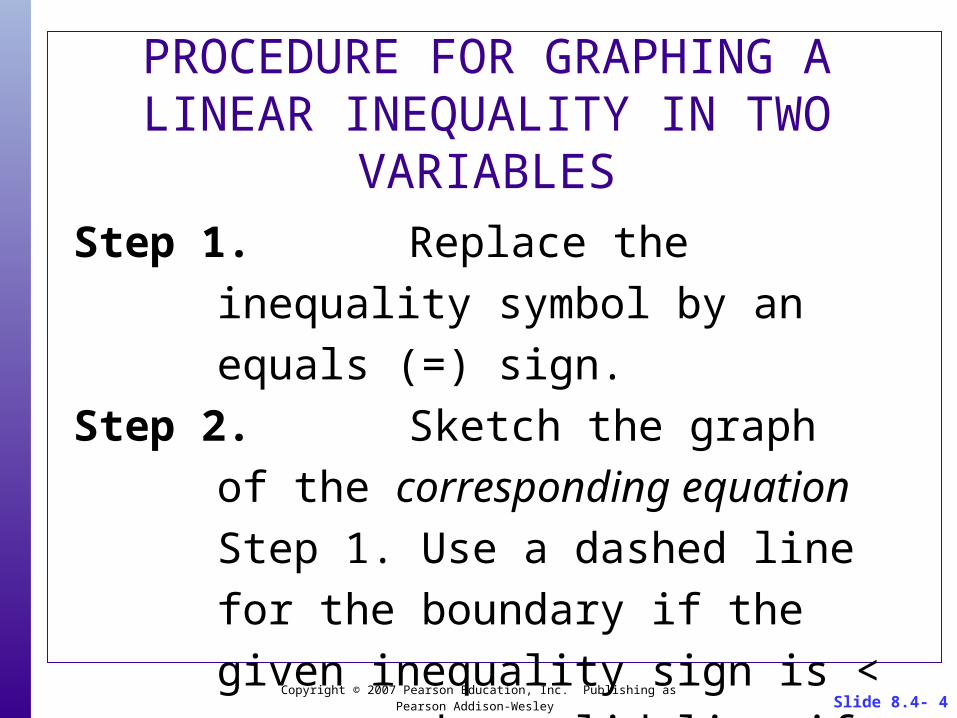
PROCEDURE FOR GRAPHING A LINEAR INEQUALITY IN TWO VARIABLES
Step 1. Replace the inequality symbol by an
equals (=) sign.
Step 2. Sketch the graph of the corresponding
equation Step 1. Use a dashed line for
the boundary if the given inequality
sign is < or >, and a solid line if the
inequality symbol is ≤ or ≥.

Slide 8.4- 5 Copyright © 2007 Pearson Education, Inc. Publishing as Pearson Addison-Wesley
PROCEDURE FOR GRAPHING A LINEAR INEQUALITY IN TWO VARIABLES
Step 3. The graph in Step 2 will divide the
plane into two regions. Select a test
point in the plane. Be sure that the test
point does not lie on the graph of the
equation in Step 1.
Step 4. (i) If the coordinates of the test point
satisfy the given inequality, then so do
all the points of the region that contains
Slide 8.4- 6 Copyright © 2007 Pearson Education, Inc. Publishing as Pearson Addison-Wesley
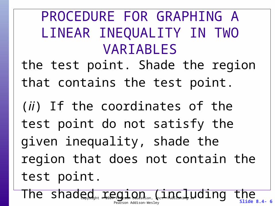
PROCEDURE FOR GRAPHING A LINEAR INEQUALITY IN TWO VARIABLES
the test point. Shade the region that contains
the test point.
(ii) If the coordinates of the test point do not
satisfy the given inequality, shade the region
that does not contain the test point.
The shaded region (including the boundary if it
is solid) is the graph of the given inequality.

Slide 8.4- 7 Copyright © 2007 Pearson Education, Inc. Publishing as Pearson Addison-Wesley
EXAMPLE 2 Graphing Inequalities
Sketch the graph of each of the following inequalities. a. x ≥ 2 b. y < 3 c. x + y < 4
Solution
a. Step 1 Change the ≥ to = : x = 2Step 2 Graph x = 2
with a solid line.Step 3 Test (0, 0). 0 ≥ 2 is a false statement.

Slide 8.4- 8 Copyright © 2007 Pearson Education, Inc. Publishing as Pearson Addison-Wesley
EXAMPLE 2 Graphing Inequalities
Solution continued
Step 3 continuedThe region not containing (0, 0), together with the vertical line, is the solution set.
Step 4 Shade the solution set.

Slide 8.4- 9 Copyright © 2007 Pearson Education, Inc. Publishing as Pearson Addison-Wesley
EXAMPLE 2 Graphing Inequalities
Solution continued
Step 2 Graph y = 3 with a dashed line.
Step 3 Test (0, 0). 0 < 3 is a true statement. The region containing (0, 0) is the solution set.
Step 4 Shade the solution set.
b. Step 1 Change the < to = : y < 3

Slide 8.4- 10 Copyright © 2007 Pearson Education, Inc. Publishing as Pearson Addison-Wesley
EXAMPLE 2 Graphing Inequalities
Solution continued
Step 2 Graph x + y = 4 with a dashed line.
Step 3 Test (0, 0). 0 < 4 is a true statement. The region containing (0, 0) is the solution set.
Step 4 Shade the solution set.
c. Step 1 Change the < to = : x + y = 4

Slide 8.4- 11 Copyright © 2007 Pearson Education, Inc. Publishing as Pearson Addison-Wesley
SYSTEMS OF LINEAR INEQUALITIES IN TWO VARIABLES
An ordered pair (a, b) is a solution of a system of inequalities involving two variables x and y if and only if, when x is replaced by a and y is replaced by b in each inequality of the system, all resulting statements are true.
The solution set of a system of inequalities is the intersection of the solution sets of all the inequalities in the system.
Slide 8.4- 12 Copyright © 2007 Pearson Education, Inc. Publishing as Pearson Addison-Wesley
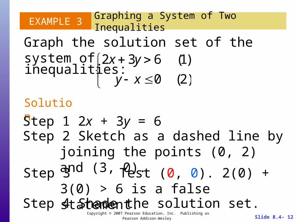
EXAMPLE 3 Graphing a System of Two Inequalities
Graph the solution set of the system of
Solution
Step 1 2x + 3y = 6Step 2 Sketch as a dashed line by joining the
points (0, 2) and (3, 0).
2x 3y 6 (1)
y x 0 (2)
inequalities:
Step 3 Test (0, 0). 2(0) + 3(0) > 6 is a false statement.
Step 4 Shade the solution set.
Slide 8.4- 13 Copyright © 2007 Pearson Education, Inc. Publishing as Pearson Addison-Wesley
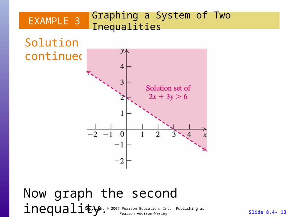
EXAMPLE 3 Graphing a System of Two Inequalities
Solution continued
Now graph the second inequality.

Slide 8.4- 14 Copyright © 2007 Pearson Education, Inc. Publishing as Pearson Addison-Wesley
EXAMPLE 3 Graphing a System of Two Inequalities
Solution continued
Step 2 Sketch as a solid line by joining the points (0, 0) and (1, 1).
Step 3 Test (1, 0). 2(0) – 3(1) > 6 is a false statement.
Step 4 Shade the solution set.
Step 1 y – x = 0

Slide 8.4- 15 Copyright © 2007 Pearson Education, Inc. Publishing as Pearson Addison-Wesley
EXAMPLE 3 Graphing a System of Two Inequalities
Solution continued
The graph of the solution set of inequalities (1) and (2) is the region where the shading overlaps.

Slide 8.4- 16 Copyright © 2007 Pearson Education, Inc. Publishing as Pearson Addison-Wesley
LINEAR PROGRAMMINGThe process of finding a maximum or minimum value of a quantity is called optimization.
A linear programming problem satisfies the following two conditions:
1. The quantity f to be maximized or minimized can be written as a linear expression in x and y. That is,
f = ax + by,where a ≠ 0, b ≠ 0 are constants.

Slide 8.4- 17 Copyright © 2007 Pearson Education, Inc. Publishing as Pearson Addison-Wesley
LINEAR PROGRAMMING
The inequalities that determine the region S are called constraints, the region S is called the set of feasible solutions, and f = ax + by is called the objective function. A point in S at which f attains its maximum (or minimum) value, together with the value of f at that point, is called an optimal solution.
2. The domain of the variables x and y is restricted to a region S that is determined by (is a solution set of) a system of linear inequalities.

Slide 8.4- 18 Copyright © 2007 Pearson Education, Inc. Publishing as Pearson Addison-Wesley
PROCEDURE FOR SOLVING A LINEAR PROGRAMMING PROBLEM
Step 1. Write an expression for the quantity to be maximized or minimized. This expression is the objective function.
Step 2. Write all constraints as linear inequalities.
Step 3. Graph the solution set of the constraint inequalities. This set is the set of feasible solutions.

Slide 8.4- 19 Copyright © 2007 Pearson Education, Inc. Publishing as Pearson Addison-Wesley
Step 4. Find all the vertices of the solution set in Step 3 by solving all pairs of corresponding equations for the constraint inequalities.
Step 5. Find the values of the objective function at each of the vertices of Step 4.
Step 6. The largest of the values (if any) in Step 5 is the maximum value of the objective function, and the smallest of the values (if any) in Step 5 is the minimum value of the objective function.

Slide 8.4- 20 Copyright © 2007 Pearson Education, Inc. Publishing as Pearson Addison-Wesley
EXAMPLE 5 Nutrition; Minimizing Calories
Fat Albert wishes to go on a crash diet and needs your help in designing a lunch menu. The menu is to include two items: soup and salad. The vitamin units (milligrams) and calorie counts in each ounce of soup and salad are given in the table.
Item Vitamin A Vitamin C Calories
SoupSalad
11
32
5040

Slide 8.4- 21 Copyright © 2007 Pearson Education, Inc. Publishing as Pearson Addison-Wesley
EXAMPLE 5 Nutrition; Minimizing Calories
Find the number of ounces of each item in the menu needed to provide the required vitamins with the fewest number of calories.
The menu must provide at least:10 units of Vitamin A24 units of Vitamin C
Solution
a. State the problem mathematically. Step 1 Write the objective function.
x = ounces of soupy = ounces of salad

Slide 8.4- 22 Copyright © 2007 Pearson Education, Inc. Publishing as Pearson Addison-Wesley
EXAMPLE 5 Nutrition; Minimizing Calories
Minimize the total number of calories. Solution continued
Step 2 Write the constraints.1 ounce soup provides 1 unit vitamin A1 ounce salad provides 1 unit vitamin ASo the total vitamin A is x + y and this must be at least 10 units so
x + y ≥ 10.
50 calories per ounce of soup: 50x40 calories per ounce of salad: 40yTotal calories = f = 50x + 40y

Slide 8.4- 23 Copyright © 2007 Pearson Education, Inc. Publishing as Pearson Addison-Wesley
EXAMPLE 5 Nutrition; Minimizing Calories
Solution continued
Step 2 Write the constraints. (continued)
1 ounce soup provides 3 units vitamin C
1 ounce salad provides 2 units vitamin C
So the total vitamin C is 3x + 2y and this
must be at least 24 units so
3x + 2y ≥ 24.
x and y cannot be negative so
x ≥ 0 and y ≥ 0.

Slide 8.4- 24 Copyright © 2007 Pearson Education, Inc. Publishing as Pearson Addison-Wesley
EXAMPLE 5 Nutrition; Minimizing Calories
Solution continued
Find x and y such that the value of f = 50x + 40y
is a minimum, with the restrictionsx y 10
3x 2y 24
x 0
y 0
b. Solve the linear programming problem.
Summarize the information.

Slide 8.4- 25 Copyright © 2007 Pearson Education, Inc. Publishing as Pearson Addison-Wesley
EXAMPLE 5 Nutrition; Minimizing Calories
Solution continued
Step 3 Graph the set of feasible solutions.
The set is bounded by
x y 10
3x 2y 24
x 0
y 0x y 10
3x 2y 24

Slide 8.4- 26 Copyright © 2007 Pearson Education, Inc. Publishing as Pearson Addison-Wesley
EXAMPLE 5 Nutrition; Minimizing Calories
Solution continued
Step 4 Find the vertices. The vertices of the feasible solutions are A(10, 0), B(4, 6) and C(0, 12).
y 0
x y 10
A (10, 0) is obtained by solving
x y 10
3x 2y 24
B (4, 6) is obtained by solving
x 0
3x 2y 24
C (0, 12) is obtained by solving

Slide 8.4- 27 Copyright © 2007 Pearson Education, Inc. Publishing as Pearson Addison-Wesley
EXAMPLE 5 Nutrition; Minimizing Calories
Solution continued
Step 5 Find the value of f at the vertices.
Vertex (x, y) Value of f = 50x + 40y
(10, 0)(4, 6)
(0, 12)
50(10) + 40(0) = 50050(4) + 40(0) = 44050(0) + 40(0) = 480
Step 6 Find the maximum or minimum value of f. The smallest value of f is 440, which occurs when x = 4 and y = 6.
Slide 8.4- 28 Copyright © 2007 Pearson Education, Inc. Publishing as Pearson Addison-Wesley
EXAMPLE 5 Nutrition; Minimizing Calories
Solution continued
c. State the conclusion
The lunch menu for Fat Albert should contain 4 ounces of soup and 6 oounces of salad. His intake of 440 calories will be as small as possible under the given constraints.