slide : in defense of smart algorithms over hardware ...as143/papers/slide_mlsys.pdfslide : in...

SLIDE : IN DEFENSE OF SMART ALGORITHMS OVER HARDWAREACCELERATION FOR LARGE-SCALE DEEP LEARNING SYSTEMS

Beidi Chen 1 Tharun Medini 1 James Farwell 2 Sameh Gobriel 2 Charlie Tai 2 Anshumali Shrivastava 1

ABSTRACTDeep Learning (DL) algorithms are the central focus of modern machine learning systems. As data volumeskeep growing, it has become customary to train large neural networks with hundreds of millions of parametersto maintain enough capacity to memorize these volumes and obtain state-of-the-art accuracy. To get around thecostly computations associated with large models and data, the community is increasingly investing in specializedhardware for model training. However, specialized hardware is expensive and hard to generalize to a multitude oftasks. The progress on the algorithmic front has failed to demonstrate a direct advantage over powerful hardwaresuch as NVIDIA-V100 GPUs. This paper provides an exception. We propose SLIDE (Sub-LInear Deep learningEngine) that uniquely blends smart randomized algorithms, with multi-core parallelism and workload optimization.Using just a CPU, SLIDE drastically reduces the computations during both training and inference outperformingan optimized implementation of Tensorflow (TF) on the best available GPU. Our evaluations on industry-scalerecommendation datasets, with large fully connected architectures, show that training with SLIDE on a 44 coreCPU is more than 3.5 times (1 hour vs. 3.5 hours) faster than the same network trained using TF on Tesla V100 atany given accuracy level. On the same CPU hardware, SLIDE is over 10x faster than TF. We provide codes andscripts for reproducibility.

1 INTRODUCTION

Deep Learning (DL) has become a topic of significant inter-est in the research community. The last few years have seena remarkable growth of using DL to significantly improvethe state-of-the-art in many applications, particularly image,text classification, and speech recognition.

The Need for Hardware Acceleration: Vast amounts ofdata powered by the exponential increase in computing ca-pabilities have been instrumental in the success of DL. Morenotably, with the advent of the powerful Graphic ProcessingUnit (GPU) (Owens et al., 2008), training processes of theDL models have been drastically accelerated.

Fast Matrix Multiplication has been heavily researched forthe past several decades. We are now reaching a limit onspeeding up matrix multiplication further. Furthermore,the need for astronomical size neural networks and un-precedented growth in the data volumes have worsenedthis problem. As a result, the community is heavily invest-ing in dedicated hardware to take DL further beyond thispoint (Jouppi et al., 2017). Designing dedicated hardware is

1Rice University 2Intel Corporation. Correspondence to: BeidiChen <[email protected]>.

Proceedings of the 3 rd MLSys Conference, Austin, TX, USA,2020. Copyright 2020 by the author(s).

risky because they require significant investment and time todevelop. Moreover, dedicated hardware caters to a specificalgorithm for which they are designed. Thus, change in thestate-of-the-art algorithms can render specialized hardwareless effective in the future. However, for the case of DL, thisinvestment is justified due to the lack of significant progressin the algorithmic alternatives for years.

Unsuccessful Alternatives to Matrix Multiplication: Onthe orthogonal side, there have been several works on replac-ing the costly matrix multiplication with cheaper algorithmicalternatives (Le Gall, 2014). Unfortunately, we have seenminimal practical benefits from the algorithmic front. So far,there has been no demonstration, even remotely, that a smartalgorithmic implementation in any form can outperform theadvantages of hardware acceleration.

Exploiting Adaptive Sparsity in Neural Networks: Inpopular frameworks like Tensorflow (TF), Sampled Soft-max (Jean et al., 2015) is deployed to approximate the fullsoftmax efficiently. While sampled softmax offers computa-tional savings, it has high estimation bias (Blanc & Rendle,2018). This leads to poor convergence behavior which isempirically verified in our experiments in section 5. In thispaper, we will exploit the idea of adaptive sparsity (Blanc &Rendle, 2018) or adaptive dropouts (Ba & Frey, 2013). Theidea stems from several recent observations (Makhzani &Frey, 2015; 2013) that we can accurately train neural net-

SLIDE : In Defense of Smart Algorithms over Hardware Acceleration for Large-Scale Deep Learning Systems

works by selectively sparsifying most of the neurons, basedon their activation, during every gradient update. (Srivas-tava et al., 2014) has also shown that selective sparsificationcan in-fact be superior in accuracy due to implicit regulariza-tion. However, selective sparsification does not directly leadto computational savings. (Spring & Shrivastava, 2017b)shows the first possibility of an algorithmically efficient so-lution by employing Locality Sensitive Hash (LSH) tablesto identify a sparse set of neurons efficiently during eachupdate. The proposed algorithm has an added advantage ofmaking the gradient update HOGWILD style parallel (Rechtet al., 2011). Such parallelism does not hurt convergence be-cause extremely sparse and independent updates are unlikelyto overlap and cause conflicts of considerable magnitude.Despite all the niceness presented, current implementationof (Spring & Shrivastava, 2017b) fails to demonstrate thatthe computational advantage can be translated into a fasterimplementation when directly compared with hardware ac-celeration of matrix multiplication. In particular, it is notclear if we can design a system that can effectively leveragethe computational advantage and at the same time compen-sate for the hash table overheads using limited (only a fewcores) parallelisms. In this paper, we provide the first suchimplementation for large fully connected neural networks.

1.1 Our Contributions

Our main contributions are as follows:

• We show the first C++ OpenMP based system SLIDEwith modest multi-core parallelism on a standard CPUthat can outperform the massive parallelism of a powerfulV100 GPU on a head-to-head time-vs-accuracy compari-son. This unique possibility is because the parallelism inSLIDE is naturally asynchronous by design. We have ourcode and benchmark scripts for reproducibility1.

• We make several novel algorithmic and data-structuralchoices in designing the LSH based sparsification tominimize the computational overheads to a few memorylookups only (truly O(1)). At the same time, it does notaffect the convergence of the DL algorithm. The imple-mentation further takes advantage of the sparse gradientupdates to achieve negligible update conflicts, which cre-ates ideal settings for Asynchronous SGD (StochasticGradient Descent) (Recht et al., 2011). These contribu-tions could be of independent interest in both the LSHand DL literature.

• We provide a rigorous evaluation of our system on twolarge benchmark datasets involving fully connected net-works. We show that SLIDE, on a modest CPU can beup to 2.7x faster, in wall clock time, than the best possi-ble alternative with the best possible choice of hardware,at any accuracy. We perform a CPU-efficiency analy-

1https://github.com/keroro824/HashingDeepLearning

sis of SLIDE using Intel VTune Performance Analyzerand show that memory-bound inefficiencies reduce forSLIDE with an increasing number of cores while it is theopposite for TF-CPU.

• Our analysis suggests that SLIDE is a memory-boundapplication, prone to some bottlenecks described in ap-pendix D. With careful workload and cache optimizations(eg. Transparent Hugepages) and a data access pattern(eg. SIMD instructions), we further speed up SLIDE byroughly 1.3x, making the overall speed up to 3.5x fasterthan TF-GPU and over 10x faster than TF-CPU.

2 LOCALITY SENSITIVE HASHING

Our paper is based on several recent and classical ideas inLocality Sensitive Hashing (LSH) and adaptive dropoutsin neural networks. LSH is a family of functions with theproperty that similar input objects in the domain of thesefunctions have a higher probability of colliding in the rangespace than non-similar ones. A popular technique for ap-proximate nearest-neighbor search uses the underlying the-ory of Locality Sensitive Hashing (Indyk & Motwani, 1998).In formal terms, considerH to be a family of hash functionsmapping RD to some set S.

Definition 2.1 (LSH Family) A familyH is called(S0, cS0, p1, p2)-sensitive if for any two points x, y ∈ RDand h chosen uniformly fromH satisfies the following:

• if Sim(x, y) ≥ S0 then Pr(h(x) = h(y)) ≥ p1• if Sim(x, y) ≤ cS0 then Pr(h(x) = h(y)) ≤ p2

Typically, for approximate nearest-neighbor search, we needp1 > p2 and c < 1 to hold. An LSH allows us to constructdata structures that give provably efficient query time algo-rithms for the approximate nearest-neighbor problem withthe associated similarity measure.

One sufficient condition for a hash familyH to be an LSHfamily is that the collision probability PrH(h(x) = h(y))should be a monotonically increasing with the similarity, i.e.

PrH(h(x) = h(y)) = f(Sim(x, y)), (1)

where f is a monotonically increasing function. In fact,most of the popular known LSH families, such as Simhash(Gionis et al., 1999) and WTA hash (Yagnik et al., 2011;Chen & Shrivastava, 2018), satisfy this strong property. Itcan be noted that Equation 1 automatically guarantees thetwo required conditions in the Definition 2.1.

It was shown in (Indyk & Motwani, 1998) that having anLSH family for a given similarity measure is sufficient for ef-ficiently solving nearest-neighbor search in sub-linear time.

The Algorithm: The LSH algorithm uses two parameters,(K,L). We construct L independent hash tables. Each


000000…11

000110…

11

h1 hk Buckets……

Empty……

LSH as Samplers

h1, h2 : RD → {0,1,2,3}

RD

h1

h2

Figure 1. Schematic diagram of LSH. For an input, we obtain hashcodes and retrieve candidates from the respective buckets.

hash table has a meta-hash function H that is formed byconcatenating K random independent hash functions fromthe collection F . Given a query, we collect one bucketfrom each hash table and return the union of L buckets.Intuitively, the meta-hash function makes the buckets sparseand reduces the number of false positives, because only validnearest-neighbor items are likely to match all K hash valuesfor a given query. The union of the L buckets decreasesthe number of false negatives by increasing the numberof potential buckets that could hold valid nearest-neighboritems. The candidate generation algorithm works in twophases [See (Spring & Shrivastava, 2017a) for details]:

1. Pre-processing Phase: We construct L hash tables fromthe data by storing all elements x. We only store pointersto the vector in the hash tables because storing wholedata vectors is very memory inefficient.

2. Query Phase: Given a query Q; we search for itsnearest-neighbors. We report the union from all of thebuckets collected from the L hash tables. Note that wedo not scan all the elements but only probe L differentbuckets, one bucket for each hash table.

After generating the set of potential candidates, the nearest-neighbor is computed by comparing the distance betweeneach item in the candidate set and the query.

2.1 LSH for Estimation and Sampling

Although LSH provides provably fast retrieval in sub-lineartime, it is known to be very slow for accurate search becauseit requires very large number of tables, i.e. large L. Also,reducing the overhead of bucket aggregation and candidatefiltering is a problem on its own. Consequent research ledto the sampling view of LSH (Spring & Shrivastava, 2017b;Chen et al., 2018; 2019; Luo & Shrivastava, 2018) thatalleviates costly searching by efficient sampling, as shownin figure 1. It turns out that merely probing a few hashbuckets (as low as 1) is sufficient for adaptive sampling.Observe that an item returned as a candidate from a (K,L)-parameterized LSH algorithm is sampled with probability1− (1− pK)L, where p is the collision probability of LSHfunction (sampling probability is monotonic in p). Thus,with LSH algorithm, the candidate set is adaptively sampledwhere the sampling probability changes with K and L.

This sampling view of LSH was the key for the algorithmproposed in paper (Spring & Shrivastava, 2017b) that showsthe first possibility of adaptive dropouts in near-constanttime, leading to efficient backpropagation algorithm.

2.1.1 MIPS Sampling

Recent advances in maximum inner product search (MIPS)using asymmetric locality sensitive hashing has made itpossible to sample large inner products. Given a col-lection C of vectors and query vector Q, using (K,L)-parameterized LSH algorithm with MIPS hashing (Shrivas-tava & Li, 2014a), we get a candidate set S. Every elementin xi ∈ C gets sampled into S with probability pi, where piis a monotonically increasing function of Q · xi. Thus, wecan pay a one-time linear cost of preprocessing C into hashtables, and any further adaptive sampling for query Q onlyrequires few hash lookups.

Algorithm 1 SLIDE Algorithm1: Input: data X , iterations n, batch size B2: Output: θ3: Initialize weights wl for each layer l4: Create hash tables HTl, functions hl for each layer l5: Compute hl(wal ) for all neurons6: Insert all neuron ids a, into HTl according to hl(wal )7: for i = 1 : n do8: Input0 = Batch(X,B)9: for l = 1 : Layers do

10: Sl = Sample(Inputl−1, HTl, hl) (Algorithm 2)11: Activation = Forward Propagation (Inputl−1, Sl)12: Inputl = Activation13: end for14: for l = 1 : Layers do15: Backpropagation (Sl)16: end for17: end for18: return θ

Algorithm 2 Algorithm for LSH Sampling1: Input: Q, HT , h2: Output: Sl (a set of active neurons on layer l)3: Compute h(Q).4: for t = 1 : L do5: S = S∩ Query(hl(Ql), HT tl )6: end for7: return S

3 PROPOSED SYSTEM: SLIDE3.1 Introduction to the overall system

Before introducing SLIDE in details, we define importantnotations: 1) B: input batch size 2) N j

l : Neuron j in layer l


12345

1234

1234

InputHidden1 Hidden2

1

5

……

…

9

Output

Layer

Active Inputs

1 0 1 ……Active Inputs

0.1 0.2 0.5 ……Activation for each Inputs

0.3 0.8 0.7 ……

Accumulated Gradients

-0.3 …Weights

0.8 -0.5

BatchSize

NeuronNetwork

HashTable1 HashTableL

00

00

00…

11

…

…

…

…

…

00

01

10…

11

ℎ"" ℎ#"… Buckets…

…

Empty…

…

…1 92

00

00

00…

11

…

…

…

…

…

00

01

10…

11

ℎ"$ ℎ#$… Buckets…

…

Empty…

…

19

5

1

2

…Previous Layer Size

Figure 2. Architecture: The central module of SLIDE is Network. The network is composed of few-layer modules. Each layer module iscomposed of neurons and a few hash tables into which the neuron ids are hashed. Each neuron module has multiple arrays of batch sizelength: 1) a binary array suggesting whether this neuron is active for each input in the batch 2) activation for each input in the batch 3)accumulated gradients for each input in the batch. 4) The connection weights to the previous layer. The last array has a length equal to thenumber of neurons in the previous layer.

3) xl: inputs for layer l in the network 4) wal : weights forath neuron in layer l 5) hl: hash functions in layer l 6) Na

l :the set of active neurons in layer l for the current input.

Initialization: Figure 2 shows the modular structure ofSLIDE and algorithm 1 shows the detailed steps. Everylayer object contains a list of neurons and a set of LSHsampling hash tables. Each hash table contains ids of theneurons that are hashed into the buckets. During the net-work initialization, the weights of the network are initializedrandomly. Afterwards, K × L LSH hash functions are ini-tialized along with L hash tables for each of the layers. Forinstance, the example network in Figure 2 maintains hashtables in two hidden layers as well as the output layer. Thedetails of using various hash functions are discussed in ap-pendix A. The LSH hash codes hl(wal ) of the weight vectorsof neurons in the given layer are computed according to thehash functions. The id a of the neuron is saved into thehash buckets mapped by the LSH function hl(wal ). Thisconstruction of LSH hash tables in each layer is a one-timeoperation which can easily be parallelized with multiplethreads over different neurons in the layer independently.

Sparse Feed-Forward Pass with Hash Table Sampling:In the feed-forward phase, given a single training instance,we compute the network activation until the final layer,which gives us the output. In SLIDE, instead of calcu-lating all the activations in each layer, the input to each layerxl is fed into hash functions to compute hl(xl). The hashcodes serve as a query to retrieve ids of active (or sampled)neurons from the matching buckets in hash tables. For ex-ample, in the figure 3, h1(x1) is first computed and thenused to retrieve N2

1 and N41 as the active neurons. Only the

activations of active neurons are calculated and passed on asthe inputs to the next layer. The other activations, like thoseof N1

1 and N31 , are directly treated as 0 and never computed.

We describe our design choices that reduce the samplingoverheads significantly in section 4.1.

12345

1234

1234

1

5

InputHidden1 Hidden2

……

…

9

H1

1|12|2,43|3

H2

1|32|1,43|2

Output

ForwardPass

Figure 3. Forward Pass: Given an input, we first get the hash codeH1 for the input, query the hash table for the first hidden layer,and obtain the active neurons. We get the activations for only thisset of active neurons. We do the same for the subsequent layersand obtain a final sparse output. In practice, we use multiple hashtables per layer.

The above-described operations are performed sequentiallyin every layer, starting from the very first layer where theinput is the data itself. Even in the output layer, which hassoftmax activation, only neurons sampled from hash tablesare treated as active neurons. For softmax, for every active

neuron, we compute its output as σ(Nko ) = exowk

o∑Na

oexowk

o.

Note that the normalizing constant for softmax is no longerthe sum over all neurons but only the active ones.

Sparse Backpropagation or Gradient Update: The back-propagation step follows the feed-forward step. After com-puting the output of the network, we compare it with theknown label of the input and backpropagate the errors layer-by-layer to calculate the gradient and update the weights.Here we use the classical backpropagation message passingtype implementation rather than vector multiplication based.For every training data instance, after updating the weightsof any given neuron, the neuron propagates the partial gra-dients (using error propagation) back to only active neuronsin previous layers via the connected weights. As a result,


we never access any non-active neuron or any non-activeweight, which is not part of the feed-forward process on agiven input. This process ensures that we take full advan-tage of sparsity. Our computation over each input is onlyof the order of active neurons and weights rather than thetotal number of parameters. It should be noted that if wecompute activation for s < 1 fraction of neurons in eachlayer (on an average), the fraction of weights that needs tobe updated is s2 only, which is a significant reduction whens is small (as is the case for our experiments).

Update Hash Tables after Weight Updates: After theweights are updated, we need to modify the positions ofneurons in the hash tables accordingly. Updating neuronstypically involves deletion from the old bucket followed byan addition to the new bucket, which can be expensive. Wediscuss several design tricks that we use to overcome thisoverhead of updating hash tables in section 4.2.

OpenMP Parallelization across a Batch: For any giventraining instance, both the feed-forward and backpropaga-tion operations are sequential as they need to be performedlayer by layer. SLIDE uses usual Batch Gradient Descentwith Adam optimizer, where the batch size is generally inthe order of hundreds. Each data instance in the batch runsin a separate thread and its gradients are computed in par-allel. To ensure the independence of computation acrossdifferent threads, every neuron stores two additional arrays,each of whose length is equal to the batch size. These arrayskeep track of the input specific neuron activations and errorgradients. Every input is assigned an id, which can be usedas an index to locate its activation (or error gradient) on anyneuron. Besides, we also have a bit array at each neuron todetermine whether the particular input activates a neuron ornot. This small memory overhead is negligible for CPUsbut it ensures that the gradient computation is independentacross different instances in the batch.

The extreme sparsity and randomness in gradient updates al-low us to asynchronously parallelize the accumulation stepof the gradient across different training data without leadingto a considerable amount of overlapping updates. SLIDEheavily capitalizes on the theory of HOGWILD (Recht et al.,2011), which shows that a small amount of overlap is tol-erable. It does not hurt the convergence even if we resolvethe concurrent updates randomly. Thus, after independentlycomputing the gradients, each thread pushes the updatesdirectly to the weights asynchronously. This asynchronousupdate avoids synchronization during batch accumulationwhich is otherwise sequential in the batch.

In section 5.3, we observe that due to this asynchronouschoice, we obtain near-perfect scaling of our implemen-tation with an increasing number of cores. Such perfectscaling is particularly exciting because even highly opti-mized implementation of TF on CPUs shows poor scalingbehavior with increasing cores beyond 16 cores.

3.2 Details of Hash Functions and Hash Tables

SLIDE provides a natural trade-off between the efficiencyof retrieving active neurons and the quality of the retrievedones. To facilitate this, we have three tunable parametersK,L,B. As mentioned in section 2, L serves as the numberof hash tables. To determine which bucket to choose, we useK hash codes for each hash table. Hence, SLIDE generatesK×L randomized hash functions all belonging to one hashfamily for each layer. In every bucket in a hash table, thenumber of entries is limited to a fixed bucket size. Such alimit helps with the memory usage and also balances theload on threads during parallel aggregation of neurons.

In our implementation of SLIDE, we support four types ofhash functions from LSH family: 1) Simhash 2) WTA hash3) DWTA hash and 4) Minhash respectively. Each of thesehash families preserves different similarities and hence isuseful for various scenarios. We discuss the implementa-tion details of Simhash and DWTA hash below and othersin appendix A. SLIDE also provides the interface to addcustomized hash functions based on need.

Simhash (Gionis et al., 1999): SimHash is a popular LSHfor the cosine similarity measure. We use K × L numberof random pre-generated vectors with components takingonly three values {+1, 0,−1}. The reason behind usingonly +1s and −1s is for fast implementation. It requiresadditions rather than multiplications, thereby reducing thecomputation and speeding up the hashing process. To fur-ther optimize the cost of Simhash in practice, we can adoptthe sparse random projection idea (Li et al., 2006). A simpleimplementation is to treat the random vectors as sparse vec-tors and store their nonzero indices in addition to the signs.For instance, let the input vector for Simhash be in Rd. Sup-pose we want to maintain 1/3 sparsity, we may uniformlygenerate K ∗ L set of d/3 indices from [0, d − 1]. In thisway, the number of multiplications for one inner productoperation during the generation of the hash codes wouldsimply reduce from d to d/3. Since the random indices areproduced from one-time generation, the cost can be ignored.

DWTA hash (Chen & Shrivastava, 2018): DWTA hashtransforms the input feature space into binary codes suchthat the Hamming distance in the resulting space closely cor-relates with rank similarity measure for sparse data. We gen-erate KLm

d number of permutations and every permutationis split into d

m bins. DWTA loops through all the nonzero(NNZ) indices of the sparse input. For each of them, we up-date the current maximum index of the corresponding binsaccording to the mapping in each permutation. It should benoted that the number of comparisons and memory lookupsin this step is O(NNZ ∗ KLmd ), which is significantly moreefficient than simply applying WTA hash to sparse input.For empty bins, the densification scheme proposed in (Chen& Shrivastava, 2018) is applied.


2000 3000 4000 5000 6000 7000# Samples

10 3

10 2

10 1Time

MIPS Strategies

Vanilla SamplingTopK SamplingHard Thresholding

Figure 4. Time consumed (in seconds) for various sampling strate-gies for retrieving active neurons from hash tables.

4 REDUCING OVERHEAD

4.1 Sampling Overhead

The key idea of using LSH for adaptive sampling of neuronsis sketched in section 3.1. We have designed three strategiesto sample neurons with large activation: 1) Vanilla Sampling2) Topk Sampling 3) Hard Thresholding. We introduce themhere and discuss their utility and efficiency in appendix B.

Vanilla Sampling: Denote βl as the number of activeneurons we target to retrieve in layer l. After computingthe hash codes of the input, we randomly choose a tableand only retrieve the neurons in its corresponding bucket.We continue retrieving neurons from another random tableuntil βl neurons are selected or all the tables have beenlooked up. Let us assume we retrieve from τ tables in total.Formally, the probability that a neuron N j

l gets chosen is,Pr(N j

l ) = (pK)τ (1 − pK)L−τ , where p is the collisionprobability of the LSH function that SLIDE uses. The timecomplexity of vanilla sampling is O(βl).

TopK Sampling: In this strategy, the basic idea is to ob-tain those neurons that occur more frequently among allL hash tables. After querying with the input, we first re-trieve all the neurons from the corresponding bucket ineach hash table and aggregate their frequencies across allhash tables. The frequencies are sorted, and only the neu-rons with top βl frequencies are selected. This requiresadditional O(|Na

l |) space for maintaining the hashmap andO(|Na

l |+ |Nal |log|Na

l |) time for both sampling and sorting.

Hard Thresholding: In this strategy, we bypass the sort-ing step in TopK sampling by selecting neurons that ap-pear at least m times in the retrieved buckets. Here, theprobability that a neuron N j

l gets chosen is, Pr(N jl ) =∑L

i=m

(Li

)(pK)i(1− pK)L−i.

Figure 4 is a preview of the empirical efficiency comparisonof above three strategies shown in appendix B. We see thatVanilla sampling is a lot more time efficient than the othertwo strategies at the cost of sample quality.

Table 1. Statistics of the datasetsFeature Dim Feature Sparsity Label Dim Training Size Testing Size

Delicious-200K 782,585 0.038 % 205,443 196,606 100,095Amazon-670K 135,909 0.055 % 670,091 490,449 153,025

4.2 Updating Overhead

We introduce the following heuristics for addressing theexpensive costs of updating the hash tables:

1) Recomputing the hash codes after every gradient update iscomputationally very expensive. Therefore, we dynamicallychange the update frequency of hash tables to reduce theoverhead. Assume that we update the hash tables for thefirst time after N0 iterations. Let t − 1 be the number oftimes the hash tables have already been updated. We applyexponential decay on the update frequency such that the tth

hash table update happens on iteration∑t−1i=0 N0e

λi, whereλ is a tunable decay constant. The intuition behind thisscheme is that the gradient updates in the initial stage of thetraining are larger than those in the later stage, especiallywhile close to convergence.

2) SLIDE needs a policy for adding a new neuron to a bucketwhen it is already full. To solve such a problem, we usethe same solution in (Wang et al., 2018) that makes useof Vitters reservoir sampling algorithm (Vitter, 1985) asthe replacement strategy. It was shown that reservoir sam-pling retains the adaptive sampling property of LSH tables,making the process sound. Additionally, we implement asimpler alternative policy based on FIFO (First In First Out).

3) For Simhash, the hash codes are computed by hsignw (x) =sign(wTx). During backpropagation, only the weights con-necting the active neurons across layers get updated. Onlythose weights contribute to the change of wTx. Therefore,we can also memorize the result of wTx besides the hashcodes. When x ∈ Rd gets updated in only d

′out of d di-

mensions, where d′ � d, we only need O(d

′) rather than

O(d) addition operations to compute the new hash codes.

5 EVALUATIONS

In this section, we’re going to empirically investigateSLIDE’s performance on multiple fronts such as: 1) SLIDEagainst TF-GPU with V100s 2) SLIDE against TF-CPU 3)SLIDE’s adaptive sampling against sampled softmax (plainrandom sampling) 4) Scalability against TF-CPU with CPUcore count 5) Effect of batch size 6) Benefits of DesignChoices. While we focus on evaluating the basic aspectsof SLIDE, we additionally perform several CPU optimiza-tions like support for Kernel Hugepages to reduce cachemisses which improve SLIDE’s performance by ≈ 30%.The optimization details are given in appendix D and theimprovement in performance is shown in section 5.4.

Fully-Connected Large Architecture: Fully connectednetworks are common in most applications. To show


102 103

Time (s)

0.25

0.30

0.35

0.40

0.45

Accu

racy

Delicious-200K

SLIDE CPUTF-GPUTF-CPU

102 103Iterations

0.25

0.30

0.35

0.40

0.45

Accuracy

Delicious-200K

SLIDE CPUTF-GPU

103 104 105Time (s)

0.05

0.10

0.15

0.20

0.25

0.30

Accuracy

Amazon-670KSLIDE CPUTF-GPUTF-CPU

103 104

Iterations

0.05

0.10

0.15

0.20

0.25

0.30

Accu

racy

Amazon-670KSLIDE CPUTF-GPU

Figure 5. It shows the comparison of SLIDE (in red) against TF-GPU (in blue) and TF-CPU (in black). The x-axis is plotted in log scaleto accommodate the otherwise slow TF-CPU curve. We notice that the time required for convergence is 2.7x lower than that of TF-GPU.When compared against iterations, the convergence behavior is identical, which confirms that the superiority of SLIDE is due to algorithmand implementation and not due to any optimization bells and whistles.

SLIDE’s real advantage, we will need large networks whereeven a slight decrease in performance is noticeable. Thus,the publicly available extreme classification datasets, requir-ing more than 100 million parameters to train due to theirextremely wide last layer, fit this setting appropriately. Forthese tasks, most of the computations (more than 99%) arein the final layer.

Datasets: We employ two large real datasets, Delicious-200K and Amazon-670K, from the Extreme ClassificationRepository (Kush Bhatia). Delicious-200K dataset is a sub-sampled dataset generated from a vast corpus of almost150 million bookmarks from Social Bookmarking Systems(del.icio.us). Amazon-670K dataset is a product to productrecommendation dataset with 670K labels. The statistics ofthe datasets are included in Table 5.

Infrastructure: All the experiments are conducted on aserver equipped with two 22-core/44-thread processors (In-tel Xeon E5-2699A v4 2.40GHz) and one NVIDIA TeslaV100 Volta 32GB GPU. The server has an Ubuntu 16.04.5LTS system with the installation of TF-GPU 1.12. We com-piled TF-CPU 1.12 from source with GCC5.4 in order tosupport FMA, AVX, AVX2, SSE4.1, and SSE4.2 instruc-tions, which boost the performance of TF-CPU by about35%. SLIDE is written in C++ and compiled under GCC5.4with OpenMP flag. The most exciting part is that SLIDEonly uses vanilla CPU thread parallelism and yet outper-forms TF-GPU (V100) by a large margin in performance.

Baselines: We benchmark the tasks with our system SLIDE,and compare against highly optimized TF framework forboth CPU and GPU. Specifically, the comparison is betweenthe same tasks, with the exact same architecture, runningon TF-CPU and TF-GPU. The optimizer and the learninghyperparameters (details later) were also the same to avoidunfair comparisons. Most of the computations in our archi-tecture are in the softmax layer. Hence, to corroborate theadvantage of adaptive sampling (Yen et al., 2018) vs vanillasampling, we also compare against the popular sampledsoftmax algorithm (Jean et al., 2015) which is a fast proxy

to the full softmax. We use the optimized Sampled Softmaxfunctionality provided in TF-GPU. This comparison shedslight on the necessity of LSH based input dependent adap-tive sampling compared to static sampling scheme which isthe only other alternative in practice.

Hyper Parameters: For both the datasets, we adopt thesame model architecture in (Yen et al., 2018). We choosethe standard fully connected neural network with one hid-den layer of size 128. We choose a batch size of 128 forDelicious-200K dataset and 256 for Amazon-670K datasetas the input dimension for the former is very large. We runall algorithms until convergence. To quantify the superiorityof SLIDE over other baselines, we also use the same opti-mizer, Adam (Kingma & Ba, 2014) by varying the initialstep size from 1e−5 to 1e−3 which leads to better conver-gence in all experiments. For SLIDE, we maintain the hashtables for the last layer, where we have a computational bot-tleneck of the models. For specific LSH setting, we chooseSimhash, K = 9, L = 50 for Delicious dataset and DWTAhash, K = 8, L = 50 for Amazon-670k dataset. We updatethe hash tables with an initial update period of N0 = 50iterations and then exponentially decaying (section 4.2).

Main Results: We show the time and iteration wise com-parisons for SLIDE vs TF GPU/CPU in Figure 5. Note thatthe x-axis is in log-scale, and all the curves have a long flatconverged portion when plotted on a linear scale indicat-ing clear convergence behavior. Red, blue and black linesrepresent the performance of SLIDE, TF-GPU, TF-CPU,respectively. We can see from the plots that SLIDE on CPUachieves any accuracy faster than TF on V100. TF-GPUis always faster than TF-CPU which is expected. It shouldbe noted that these datasets are very sparse, e.g., Deliciousdataset has only 75 non-zeros on an average for input fea-tures, and hence the advantage of GPU over CPU is notalways noticeable.

SLIDE is around 1.8 times faster than TF-GPU on Delicious200k. On the larger Amazon 670k dataset, where we needmore computations, the gains are substantially more. SLIDE


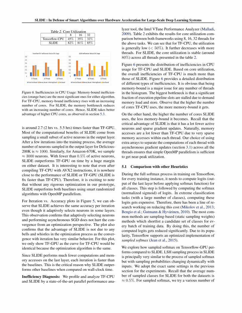
Table 2. Core Utilization8 16 32

Tensorflow-CPU 45% 35% 32%SLIDE 82% 81% 85%

0

0.1

0.2

0.3

0.4

0.5

0.6

8Threads 16Threads 32Threads

Tensorflow-CPU Inefficiencies Ratio in CPU Usage

Front-EndBound MemoryBound RetiringBound CoreBound

0

0.1

0.2

0.3

0.4

0.5

0.6

8Threads 16Threads 32Threads

SLIDEInefficiencies Ratio in CPU Usage

Front-EndBound MemoryBound RetiringBound CoreBound

Figure 6. Inefficiencies in CPU Usage: Memory-bound inefficien-cies (orange bars) are the most significant ones for either algorithm.For TF-CPU, memory-bound inefficiency rises with an increasingnumber of cores. For SLIDE, the memory bottleneck reduceswith an increasing number of cores. Hence, SLIDE takes betteradvantage of higher CPU cores, as observed in section 5.3.

is around 2.7 (2 hrs vs. 5.5 hrs) times faster than TF-GPU.Most of the computational benefits of SLIDE come fromsampling a small subset of active neurons in the output layer.After a few iterations into the training process, the averagenumber of neurons sampled in the output layer for Delicious-200K is ≈ 1000. Similarly, for Amazon-670K, we sample≈ 3000 neurons. With fewer than 0.5% of active neurons,SLIDE outperforms TF-GPU on time by a huge marginon either dataset. It is interesting to note that even aftercompiling TF-CPU with AVX2 instructions, it is nowhereclose to the performance of SLIDE or TF-GPU (SLIDE is8x faster than TF-CPU). Therefore, it is exciting to notethat without any rigorous optimization in our prototype,SLIDE outperforms both baselines using smart randomizedalgorithms with OpenMP parallelism.

For Iteration vs. Accuracy plots in Figure 5, we can ob-serve that SLIDE achieves the same accuracy per iterationeven though it adaptively selects neurons in some layers.This observation confirms that adaptively selecting neuronsand performing asynchronous SGD does not hurt the con-vergence from an optimization perspective. The plot alsoconfirms that the advantage of SLIDE is not due to anybells and whistles in the optimization process as the conver-gence with iteration has very similar behavior. For this plot,we only show TF-GPU as the curve for TF-CPU would beidentical because the optimization algorithm is the same.

Since SLIDE performs much fewer computations and mem-ory accesses on the last layer, each iteration is faster thanthe baselines. This is the critical reason why SLIDE outper-forms other baselines when compared on wall-clock time.

Inefficiency Diagnosis: We profile and analyze TF-CPUand SLIDE by a state-of-the-art parallel performance ana-

lyzer tool, the Intel VTune Performance Analyzer (Malladi,2009). Table 2 exhibits the results for core utilization com-parison between both frameworks using 8, 16, 32 threads forthe above tasks. We can see that for TF-CPU, the utilizationis generally low (< 50%). It further decreases with morethreads. For SLIDE, the core utilization is stable (around80%) across all threads presented in the table 2.

Figure 6 presents the distribution of inefficiencies in CPUusage for TF-CPU and SLIDE. Based on core utilization,the overall inefficiencies of TF-CPU is much more thanthose of SLIDE. Figure 6 provides a detailed distributionof different types of inefficiencies. It is obvious that beingmemory-bound is a major issue for any number of threadsin the histogram. The biggest bottleneck is that a significantfraction of execution pipeline slots are stalled due to demandmemory load and store. Observe that the higher the numberof cores TF-CPU uses, the more memory-bound it gets.

On the other hand, the higher the number of cores SLIDEuses, the less memory-bound it becomes. Recall that thecritical advantage of SLIDE is that it has a lot fewer activeneurons and sparse gradient updates. Naturally, memoryaccesses are a lot fewer than TF-CPU due to very sparsememory accesses within each thread. Our choice of usingextra arrays to separate the computations of each thread withasynchronous gradient updates (section 3.1) across all thethreads ensures that simple OpenMP parallelism is sufficientto get near-peak utilization.

5.1 Comparison with other Heuristics

During the full softmax process in training on Tensorflow,for every training instance, it needs to compute logits (out-put of the last layer before applying softmax function) forall classes. This step is followed by computing the softmax(normalized sigmoid) of logits. In extreme classificationtasks (with a large number of classes), computing theselogits gets expensive. Therefore, there has been a line of re-search working on reducing this cost (Mikolov et al., 2013;Bengio et al.; Gutmann & Hyvarinen, 2010). The most com-mon methods are sampling-based (static sampling weights)methods which shortlist a candidate set of classes for ev-ery batch of training data. By doing this, the number ofcomputed logits gets reduced significantly. Due to its popu-larity, Tensorflow supports an optimized implementation ofsampled softmax (Jean et al., 2015).

We explore how sampled softmax on Tensorflow-GPU per-forms compared to SLIDE. LSH sampling process in SLIDEis principally very similar to the process of sampled softmaxbut with sampling probabilities changing dynamically withinputs. We adopt the exact same settings in the previoussection for the experiments. Recall that the average num-ber of sampled classes for SLIDE for both the datasets is≈ 0.5%. For sampled softmax, we try a various number of


102 103

Time (s)

0.050.100.150.200.250.300.350.400.45

Accu

racy

Delicious-200K

SLIDE CPUTF-GPU SSM

102 103 104

Iterations

0.050.100.150.200.250.300.350.400.45

Accu

racy

Delicious-200K

SLIDE CPUTF-GPU SSM

102 103 104Time (s)

0.00

0.05

0.10

0.15

0.20

0.25

0.30

Accuracy

Amazon-670KSLIDE CPUTF-GPU SSM

103 104 105

Iterations

0.00

0.05

0.10

0.15

0.20

0.25

0.30

Accu

racy

Amazon-670KSLIDE CPUTF-GPU SSM

Figure 7. It shows the comparison of SLIDE (in red) against the popular Sampled Softmax heuristic (in green). The plots clearly establishthe limitations of Sampled Softmax. On Amazon-670K dataset, we notice that Sampled Softmax starts to grow faster than SLIDE in thebeginning stages of training but saturates quickly to lower accuracy. SLIDE starts to grow slowly but attains much higher accuracy thanSampled Softmax. SLIDE has the context of choosing the most informative neurons at each layer. Sampled Softmax always chooses arandom subset of neurons in the final layer. This reflects in the superior performance of SLIDE over Sampled Softmax.

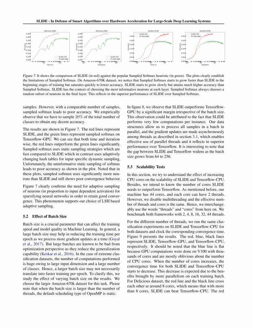
samples. However, with a comparable number of samples,sampled softmax leads to poor accuracy. We empiricallyobserve that we have to sample 20% of the total number ofclasses to obtain any decent accuracy.

The results are shown in Figure 7. The red lines representSLIDE, and the green lines represent sampled softmax onTensorflow-GPU. We can see that both time and iterationwise, the red lines outperform the green lines significantly.Sampled softmax uses static sampling strategies which arefast compared to SLIDE which in contrast uses adaptivelychanging hash tables for input specific dynamic sampling.Unfortunately, the uninformative static sampling of softmaxleads to poor accuracy as shown in the plot. Noted that inthese plots, sampled softmax uses significantly more neu-rons than SLIDE and still shows poor convergence behavior.

Figure 7 clearly confirms the need for adaptive samplingof neurons (in proportion to input dependent activation) forsparsifying neural networks in order to retain good conver-gence. This phenomenon supports our choice of LSH basedadaptive sampling.

5.2 Effect of Batch Size

Batch size is a crucial parameter that can affect the trainingspeed and model quality in Machine Learning. In general, alarge batch size may help in reducing the training time perepoch as we process more gradient updates at a time (Goyalet al., 2017). But large batches are known to be bad fromoptimization perspective as they reduce the generalizationcapability (Keskar et al., 2016). In the case of extreme clas-sification datasets, the number of computations performedis huge owing to large input dimension and a large numberof classes. Hence, a larger batch size may not necessarilytranslate into faster training per epoch. To clarify this, westudy the effect of varying batch size on the results. Wechoose the larger Amazon-670k dataset for this task. Pleasenote that when the batch size is larger than the number ofthreads, the default scheduling type of OpenMP is static.

In figure 8, we observe that SLIDE outperforms Tensorflow-GPU by a significant margin irrespective of the batch size.This observation could be attributed to the fact that SLIDEperforms very few computations per instance. Our datastructures allow us to process all samples in a batch inparallel, and the gradient updates are made asynchronouslyamong threads as described in section 3.1, which enableseffective use of parallel threads and it reflects in superiorperformance over Tensorflow. It is interesting to note thatthe gap between SLIDE and Tensorflow widens as the batchsize grows from 64 to 256.

5.3 Scalability Tests

In this section, we try to understand the effect of increasingCPU cores on the scalability of SLIDE and Tensorflow-CPU.Besides, we intend to know the number of cores SLIDEneeds to outperform Tensorflow. As mentioned before, ourmachine has 44 cores, and each core can have 2 threads.However, we disable multithreading and the effective num-ber of threads and cores is the same. Hence, we interchange-ably use the words “threads” and “cores” from here on. Webenchmark both frameworks with 2, 4, 8, 16, 32, 44 threads.

For the different number of threads, we run the same clas-sification experiments on SLIDE and Tensorflow-CPU forboth datasets and clock the corresponding convergence time.Figure 9 presents the results. The red, blue, black linesrepresent SLIDE, Tensorflow-GPU, and Tensorflow-CPU,respectively. It should be noted that the blue line is flatbecause GPU computations were done on V100 with thou-sands of cores and are mostly oblivious about the numberof CPU cores. When the number of cores increases, theconvergence time for both SLIDE and Tensorflow-CPUstarts to decrease. This decrease is expected due to the ben-efits brought by more parallelism on each training batch.For Delicious dataset, the red line and the black line crosseach other at around 8 cores, which means that with morethan 8 cores, SLIDE can beat Tensorflow-CPU. The red


102 103 104

Time (s)

0.00

0.05

0.10

0.15

0.20

0.25

0.30Ac

curacy

Amazon-670K, Batch_Size=64SLIDE CPUTF-GPUTF-GPU SSM

102 103 104

Time (s)

0.00

0.05

0.10

0.15

0.20

0.25

0.30

Accuracy


102 103 104

Time (s)

0.00

0.05

0.10

0.15

0.20

0.25

0.30

0.35

Accu

racy


Figure 8. Performance of SLIDE vs. Tensorflow-GPU vs. Sampled Softmax at different batch sizes. SLIDE outperforms the baselines atall batch sizes. As the batch size gets larger, the gap between SLIDE and TF-GPU gets wider.

21 22 23 24 25# Cores

103Conv

erge

nce Time

Delicious-200KSLIDETF-CPUTF-GPU

21 22 23 24 25

# Cores

104

105

Conv

erge

nce

Tim

e

Amazon-670KSLIDETF-CPUTF-GPU

Figure 9. Scalability Tests: Comparison of performance gains withthe number of CPU cores for SLIDE (in red ) vs. Tensorflow-CPU (in black) vs. Tensorflow-GPU (in blue). The blue lineis flat because the performance of TF-GPU does not depend onCPU cores. We notice that the convergence time drops steeply forSLIDE compared to TF-CPU/GPU. On Delicious-200K dataset,SLIDE beats TF-CPU with just 8 cores and TF-GPU with lessthan 32 cores. Similarly, on Amazon-670K dataset, SLIDE beatsTF-CPU with just 2 cores and TF-GPU with just 8 cores.

and blue lines intersect between 16 and 32 cores. Hence,with fewer than 32 cores, SLIDE outperforms Tensorflow-GPU on Delicious dataset. Similarly, for larger Amazondataset, the red and black line never intersect, and the redand blue line intersects on 8 cores. This means that SLIDEbeats Tensorflow-GPU with as few as 8 CPU cores andTensorflow-CPU with as few as 2 CPU cores.

5.4 Additional Speedup with Threading Model andPlatform Micro-architecture

In this section, we perform several CPU optimizations out-lined in appendix D to reduce cache misses. We first installHugepages package for Ubuntu, which offers 2MB and1GB cache pages in addition to default 4KB ones. Wepre-allocate 1000 2MB Hugepages and 10 1GB Hugepageswhich are found to be enough for both Delicious-200K andAmazon-670K datasets. To resolve the issue of the falsesharing for OpenMP mutli-thread, we give a provision toour data structures to align on cache line boundaries. Be-sides using Hugepages, we also used SIMD instructions(specifically, Intel-AVX) to facilitate per thread batching.In figure 10, we compare the benefit of aforementioned op-timizations against an un-optimized SLIDE and TF-GPU.

103 104Time (s)

0.05

0.10

0.15

0.20

0.25

0.30

Accuracy

Amazon-670K

SLIDE-CPUSLIDE-CPU OptimizedTF-GPU

102 103Time (s)

0.25

0.30

0.35

0.40

0.45

Accuracy

Delicious-200K

SLIDE-CPUSLIDE-CPU OptimizedTF-GPU

Figure 10. Impact of Hugepages and SIMD Optimization: Thecomparison of training time for optimized version of SLIDEagainst a plain version of SLIDE and TF-GPU. We can see thatSLIDE-Optimized is roughly 1.3x faster than the un-optimizedone on both datasets (x-axis is log scale).

We notice that Cache-Optimized SLIDE (in green) is ≈ 1.3times faster than basic SLIDE (in red). Since we alreadyhave a 2.7x speed-up over TF-GPU on Amazon-670K, ittranslates to 3.5x speedup over TF-GPU and a 10x speedupover TF-CPU.

In appendix D.1, we measure the impact of HugePageson various CPU-counter metrics like TLB miss rates andPageFaults. Concisely, we notice that HugePages reducesthe misses by a large margin.

6 CONCLUSION AND FUTURE WORK

We provide the first evidence that a smart algorithm withmodest CPU OpenMP parallelism can outperform the bestavailable hardware NVIDIA-V100, for training large deeplearning architectures. Our system SLIDE is a combinationof carefully tailored randomized hashing algorithms withthe right data structures that allow asynchronous parallelism.We show up to 3.5x gain against TF-GPU and 10x gainagainst TF-CPU in training time with similar precision onpopular extreme classification datasets. Our next steps are toextend SLIDE to include convolutional layers. SLIDE hasunique benefits when it comes to random memory accessesand parallelism. We anticipate that a distributed imple-mentation of SLIDE would be very appealing because thecommunication costs are minimal due to sparse gradients.


7 ACKNOWLEDGEMENTS

The work was supported by NSF-1652131, NSF-BIGDATA1838177, AFOSR-YIPFA9550-18-1-0152, Amazon Re-search Award, and ONR BRC grant for Randomized Nu-merical Linear Algebra.

REFERENCES

Ba, J. and Frey, B. Adaptive dropout for training deep neuralnetworks. In Advances in Neural Information ProcessingSystems, pp. 3084–3092, 2013.

Basu, A., Gandhi, J., Chang, J., Hill, M., and Swift, M.Efficient virtual memory for big memory servers. InInternational Symposium on Computer Architecture, pp.237–248, 2013.

Bengio, Y. et al. Quick training of probabilistic neural netsby importance sampling.

Blanc, G. and Rendle, S. Adaptive sampled softmax withkernel based sampling. In International Conference onMachine Learning, pp. 589–598, 2018.

Chen, B. and Shrivastava, A. Densified winner take all (wta)hashing for sparse datasets. In Uncertainty in artificialintelligence, 2018.

Chen, B., Shrivastava, A., and Steorts, R. C. Unique entityestimation with application to the syrian conflict. THEANNALS, 2018.

Chen, B., Xu, Y., and Shrivastava, A. Fast and accuratestochastic gradient estimation. In Advances in NeuralInformation Processing Systems, pp. 12339–12349, 2019.

Corbet, J. Transparent huge pages in 2.6.38.http://lwn.net/Articles/423584/, 2011.

Gionis, A., Indyk, P., and Motwani, R. Similarity searchin high dimensions via hashing. In Proceedings of the25th International Conference on Very Large Data Bases,VLDB ’99, pp. 518–529, San Francisco, CA, USA, 1999.Morgan Kaufmann Publishers Inc. ISBN 1-55860-615-7. URL http://dl.acm.org/citation.cfm?id=645925.671516.

Goyal, P., Dollar, P., Girshick, R., Noordhuis, P.,Wesolowski, L., Kyrola, A., Tulloch, A., Jia, Y., andHe, K. Accurate, large minibatch sgd: Training imagenetin 1 hour. arXiv preprint arXiv:1706.02677, 2017.

Gutmann, M. and Hyvarinen, A. Noise-contrastive esti-mation: A new estimation principle for unnormalizedstatistical models. In Proceedings of the Thirteenth Inter-national Conference on Artificial Intelligence and Statis-tics, pp. 297–304, 2010.

Hasabnis, N. Auto-tuning tensorflow threading model forCPU backend. CoRR, abs/1812.01665, 2018. URLhttp://arxiv.org/abs/1812.01665.

Indyk, P. and Motwani, R. Approximate nearest neigh-bors: towards removing the curse of dimensionality. InProceedings of the thirtieth annual ACM symposium onTheory of computing, pp. 604–613. ACM, 1998.

Jean, S., Cho, K., Memisevic, R., and Bengio, Y. On usingvery large target vocabulary for neural machine transla-tion. In Proceedings of the 53rd Annual Meeting of theAssociation for Computational Linguistics and the 7thInternational Joint Conference on Natural Language Pro-cessing (Volume 1: Long Papers), volume 1, pp. 1–10,2015.

Jouppi, N. P., Young, C., Patil, N., Patterson, D., Agrawal,G., Bajwa, R., Bates, S., Bhatia, S., Boden, N., Borchers,A., et al. In-datacenter performance analysis of a tensorprocessing unit. In 2017 ACM/IEEE 44th Annual Inter-national Symposium on Computer Architecture (ISCA),pp. 1–12. IEEE, 2017.

Karakostas, V., Unsal, O., Nemirovsky, M., Cristal, A.,and Swift, M. Performance analysis of the memorymanagement unit under scale-out workloads. In Inter-national Symposium on Workload Characterization, pp.1–12, 2014.

Keskar, N. S., Mudigere, D., Nocedal, J., Smelyanskiy,M., and Tang, P. T. P. On large-batch training for deeplearning: Generalization gap and sharp minima. arXivpreprint arXiv:1609.04836, 2016.

Kingma, D. P. and Ba, J. Adam: A method for stochasticoptimization. arXiv preprint arXiv:1412.6980, 2014.

Kumar, A., Soltis, D., Esmer, I., Yoaz, I., and Kottapalli, S.The new intel xeon scalable processor(formerly skylake-sp). In Hot Chips, 2017.

Kush Bhatia, Kunal Dahiya, H. J. Y. P. M. V. Theextreme classification repository: Multi-label datasetscode. http://manikvarma.org/downloads/XC/XMLRepository.html#Prabhu14.

Le Gall, F. Powers of tensors and fast matrix multiplication.In Proceedings of the 39th international symposium onsymbolic and algebraic computation, pp. 296–303. ACM,2014.

Li, P., Hastie, T. J., and Church, K. W. Very sparse randomprojections. In Proceedings of the 12th ACM SIGKDDinternational conference on Knowledge discovery anddata mining, pp. 287–296. ACM, 2006.

http://dl.acm.org/citation.cfm?id=645925.671516

http://dl.acm.org/citation.cfm?id=645925.671516

http://arxiv.org/abs/1812.01665

http://manikvarma.org/downloads/XC/XMLRepository.html#Prabhu14

http://manikvarma.org/downloads/XC/XMLRepository.html#Prabhu14


Luo, C. and Shrivastava, A. Scaling-up split-merge mcmcwith locality sensitive sampling (lss). arXiv preprintarXiv:1802.07444, 2018.

Makhzani, A. and Frey, B. K-sparse autoencoders. arXivpreprint arXiv:1312.5663, 2013.

Makhzani, A. and Frey, B. J. Winner-take-all autoencoders.In Advances in neural information processing systems,pp. 2791–2799, 2015.

Malladi, R. K. Using intel R© vtune performance analyzerevents/ratios & optimizing applications. http:/software.intel. com, 2009.

Meng, J. and Skadron, K. Avoiding cache thrashing due toprivate data placement in last-level cache for manycorescaling. In International Conference on Computer Design,pp. 283–297, 2009.

Mikolov, T., Sutskever, I., Chen, K., Corrado, G. S., andDean, J. Distributed representations of words and phrasesand their compositionality. In Advances in neural infor-mation processing systems, pp. 3111–3119, 2013.

Owens, J. D., Houston, M., Luebke, D., Green, S., Stone,J. E., and Phillips, J. C. Gpu computing. 2008.

Recht, B., Re, C., Wright, S., and Niu, F. Hogwild: A lock-free approach to parallelizing stochastic gradient descent.In Advances in neural information processing systems,pp. 693–701, 2011.

Shrivastava, A. and Li, P. Asymmetric lsh (alsh) for sub-linear time maximum inner product search (mips). InAdvances in Neural Information Processing Systems, pp.2321–2329, 2014a.

Shrivastava, A. and Li, P. Densifying one permutationhashing via rotation for fast near neighbor search. InInternational Conference on Machine Learning, pp. 557–565, 2014b.

Spring, R. and Shrivastava, A. A new unbiased and efficientclass of lsh-based samplers and estimators for partitionfunction computation in log-linear models. arXiv preprintarXiv:1703.05160, 2017a.

Spring, R. and Shrivastava, A. Scalable and sustainabledeep learning via randomized hashing. In Proceedingsof the 23rd ACM SIGKDD International Conference onKnowledge Discovery and Data Mining, pp. 445–454.ACM, 2017b.

Srivastava, N., Hinton, G., Krizhevsky, A., Sutskever, I.,and Salakhutdinov, R. Dropout: a simple way to preventneural networks from overfitting. The Journal of MachineLearning Research, 15(1):1929–1958, 2014.

Vitter, J. S. Random sampling with a reservoir. ACMTransactions on Mathematical Software (TOMS), 11(1):37–57, 1985.

Wang, Y., Shrivastava, A., Wang, J., and Ryu, J. Random-ized algorithms accelerated over cpu-gpu for ultra-highdimensional similarity search. In ACM SIGMOD Record,pp. 889–903. ACM, 2018.

Wicaksono, B., Tolubaeva, M., and Chapman, B. Detectingfalse sharing in openmp applications using the darwinframework. In Lecture Notes in Computer Science, pp.282–288, 2011.

Yagnik, J., Strelow, D., Ross, D. A., and Lin, R.-s. Thepower of comparative reasoning. In 2011 InternationalConference on Computer Vision, pp. 2431–2438. IEEE,2011.

Yen, I. E.-H., Kale, S., Yu, F., Holtmann-Rice, D., Kumar, S.,and Ravikumar, P. Loss decomposition for fast learningin large output spaces. In International Conference onMachine Learning, pp. 5626–5635, 2018.

A DIFFERENT HASH FUNCTIONS

Signed Random Projection (Simhash) : Refer (Gioniset al., 1999) for explanation of the theory behind Simhash.We use K × L number of random pre-generated vectorswith components taking only three values {+1, 0,−1}. Thereason behind using only +1s and −1s is for fast imple-mentation. It requires additions rather than multiplications,thereby reducing the computation and speeding up the hash-ing process. To further optimize the cost of Simhash inpractice, we can adopt the sparse random projection idea (Liet al., 2006). A simple implementation is to treat the randomvectors as sparse vectors and store their nonzero indices inaddition to the signs. For instance, let the input vector forSimhash be in Rd. Suppose we want to maintain 1/3 spar-sity, we may uniformly generate K ∗ L set of d/3 indicesfrom [0, d− 1]. In this way, the number of multiplicationsfor one inner product operation during the generation of thehash codes would simply reduce from d to d/3. Since therandom indices are produced from one-time generation, thecost can be safely ignored.

Winner Takes All Hashing (WTA hash) : In SLIDE,we slightly modify the WTA hash algorithm from (Yagniket al., 2011) for memory optimization. Originally, WTAtakes O(KLd) space to store the random permutations Θgiven the input vector is in Rd. m << d is a adjustablehyper-parameter. We only generate KLm

d rather than K ∗ Lpermutations and thereby reducing the space to O(KLm).Every permutation is split into d

m parts (bins) evenly andeach of them can be used to generate one WTA hash code.


Computing the WTA hash codes also takes O(KLm) oper-ations.

Densified Winner Takes All Hashing (DWTA hash) : Asargued in (Chen & Shrivastava, 2018), when the input vectoris very sparse, WTA hashing no longer produces represen-tative hash codes. Therefore, we use DWTA hashing, thesolution proposed in (Chen & Shrivastava, 2018). Similarto WTA hash, we generate KLm

d number of permutationsand every permutation is split into d

m bins. DWTA loopsthrough all the nonzero (NNZ) indices of the sparse input.For each of them, we update the current maximum indexof the corresponding bins according to the mapping in eachpermutation.

It should be noted that the number of comparisons andmemory lookups in this step is O(NNZ ∗ KLmd ), which issignificantly more efficient than simply applying WTA hashto sparse input. For empty bins, the densification schemeproposed in (Chen & Shrivastava, 2018) is applied.

Densified One Permutation Minwise Hashing(DOPH):The implementation mostly follows the description ofDOPH in (Shrivastava & Li, 2014b). DOPH is mainly de-signed for binary inputs. However, the weights of the inputsfor each layer are unlikely to be binary. We use a thresh-olding heuristic for transforming the input vector to binaryrepresentation before applying DOPH. The k highest valuesamong all d dimensions of the input vector are convertedto 1s and the rest of them become 0s. Define idxk as theindices of the top k values for input vector x. Formally,

Threshold(xi) =

{1, if i ∈ idxk.0, otherwise.

We could use sorting algorithms to get the top k indices, butit induces at least O(dlogd) overhead. Therefore, we keepa priority queue with indices as keys and the correspondingdata values as values. This requires O(dlogk) operations.

B REDUCING THE SAMPLING OVERHEAD

The key idea of using LSH for adaptive sampling of neuronswith large activation is sketched in ‘Introduction to over-all system’ section in the main paper. We have designedthree strategies to sample large inner products: 1) VanillaSampling 2) Topk Sampling 3) Hard Thresholding. We firstintroduce them one after the other and then discuss theirutility and efficiency. Further experiments are reported insection C.

Vanilla Sampling: Denote βl as the number of activeneurons we target to retrieve in layer l. After computing thehash codes of the input, we randomly choose a table and onlyretrieve the neurons in that table. We continue retrievingneurons from another random table until βl neurons areselected or all the tables have been looked up. Let us assume

we retrieve from τ tables in total. Formally, the probabilitythat a neuron N j

l gets chosen is,

Pr(N jl ) = (pK)τ (1− pK)L−τ , (2)

where p is the collision probability of the LSH function thatSLIDE uses. For instance, if Simhash is used,

p = 1−cos−1

((wj

l )T xl

||wjl ||2·||xl||2

)π

.

From the previous process, we can see that the time com-plexity of vanilla sampling is O(βl).

TopK Sampling: In this strategy, the basic idea is to obtainthose neurons that occur more frequently among all L hashtables. After querying with the input, we first retrieve allthe neurons from the corresponding bucket in each hashtable. While retrieving, we use a hashmap to keep trackof the frequency with which each neuron appears. Thehashmap is sorted based on the frequencies, and only theneurons with top βl frequencies are selected. This requiresadditional O(|Na

l |) space for maintaining the hashmap andO(|Na

l |+ |Nal |log|Na

l |) time for both sampling and sorting.

Hard Thresholding: The TopK Sampling could be expen-sive due to the sorting step. To overcome this, we proposea simple variant that collects all neurons that occur morethan a certain frequency. This bypasses the sorting step andalso provides a guarantee on the quality of sampled neurons.Suppose we only select neurons that appear at least m timesin the retrieved buckets, the probability that a neuron N j

l

gets chosen is,

Pr(N jl ) =

L∑i=m

(Li

)(pK)i(1− pK)L−i, (3)

Figure 11 shows a sweep of curves that present the relationbetween collision probability of hl(w

jl ) and hl(xl) and the

probability that neuron N jl is selected under various values

of m when L = 10. We can visualize the trade-off betweencollecting more good neurons and omitting bad neurons bytweaking m. For a high threshold like m = 9, only theneurons with p > 0.8 have more than Pr > 0.5 chance ofretrieval. This ensures that bad neurons are eliminated butthe retrieved set might be insufficient. However, for a lowthreshold like m = 1, all good neurons are collected butbad neurons with p < 0.2 are also collected with Pr > 0.8.Therefore, depending on the tolerance for bad neurons, wechoose an intermediate m in practice.

C DESIGN CHOICE COMPARISONS

In the main paper, we presented several design choices inSLIDE which have different trade-offs and performancebehavior, e.g., executing MIPS efficiently to select active


0.1 0.2 0.3 0.4 0.5 0.6 0.7 0.8 0.9p

0.0

0.2

0.4

0.6

0.8

1.0

PrTrade off for Frequency Thresholding

m=1m=3m=5m=7m=9

Figure 11. Hard Thresholding: Theoretical selection probabilityPr vs the collision probabilities p for various values of frequencythreshold m (eqn. 3). High threshold (m = 9) gets less numberof false positive neurons but misses out on many active neurons.A low threshold (m = 1) would select most of the active neuronsalong with lot of false positives.

neurons, adopting the optimal policies for neurons insertionin hash tables, etc. In this section, we substantiate thosedesign choices with key metrics and insights. In order tobetter analyze them in more practical settings, we chooseto benchmark them in real classification tasks on Delicious-200K dataset.

C.1 Evaluating Sampling Strategies

Sampling is a crucial step in SLIDE. The quality and quan-tity of selected neurons and the overhead of the selectionstrategy significantly affect the SLIDE performance. Weprofile the running time of these strategies, including Vanillasampling, TopK thresholding, and Hard thresholding, forselecting a different number of neurons from the hash tablesduring the first epoch of the classification task.

Figure 12 presents the results. The blue, red and green dotsrepresent Vanilla sampling, TopK thresholding, and Hardthresholding respectively. It shows that the TopK thresh-olding strategy takes magnitudes more time than Vanillasampling and Hard thresholding across all number of sam-ples consistently. Also, we can see that the green dots arejust slightly higher than the blue dots meaning that the timecomplexity of Hard Thresholding is slightly higher thanVanilla Sampling. Note that the y-axis is in log scale. There-fore when the number of samples increases, the rates ofchange for the red dots are much more than those of theothers. This is not surprising because TopK thresholdingstrategy is based on sorting algorithms which has O(nlogn)running time. Therefore, in practice, we suggest choos-ing either of Vanilla Sampling or Hard Thresholding forefficiency. For instance, we use Vanilla Sampling in our

2000 3000 4000 5000 6000 7000# Samples

10 3

10 2

10 1

Time

MIPS Strategies

Vanilla SamplingTopK SamplingHard Thresholding

Figure 12. Sampling Strategies: Time consumed (in seconds) forvarious sampling methods after retrieving active neurons fromHash Tables.

extreme classification experiments because it is the mostefficient one. Furthermore, the difference between iterationwise convergence of the tasks with TopK Thresholding andVanilla Sampling are negligible.

C.2 Addition to Hashtables

SLIDE supports two implementations of insertion policiesfor hash tables described in section 3.1 in main paper. Weprofile the running time of the two strategies, ReservoirSampling and FIFO. After the weights and hash tables ini-tialization, we clock the time of both strategies for insertionsof all 205,443 neurons in the last layer of the network, where205,443 is the number of classes for Delicious dataset. Thenwe also benchmark the time of whole insertion process in-cluding generating the hash codes for each neuron beforeinserting them into hash tables.

The results are shown in Table C.2. The column “Full Inser-tion” represents the overall time for the process of adding allneurons to hash tables. The column “Insertion to HT” repre-sents the exact time of adding all the neurons to hash tablesexcluding the time for computing the hash codes. ReservoirSampling strategy is more efficient than FIFO. From an al-gorithmic view, Reservoir Sampling inserts based on someprobability, but FIFO guarantees successful insertions. Weobserve that there are more memory accesses with FIFO.However, compared to the full insertion time, the benefitsof Reservoir Sampling are still negligible. Therefore wecan choose either strategy based on practical utility. Forinstance, we use FIFO in our experiments.


Table 3. Time taken by hash table insertion schemesInsertion to HT Full Insertion

Reservoir Sampling 0.371 s 18 sFIFO 0.762 s 18 s

D THREADING MODEL AND PLATFORMMICRO-ARCHITECTUREOPTIMIZATION

Our experimental analysis shows that SLIDE is a memory-bound workload. We show that a careful workload optimiza-tion to design a threading model and a data access pattern totake into consideration the underlying platform architectureleads to a significant performance boost.

OpenMP and Cache Optimizations: A key metric forthe identification of memory and cache performance bottle-necks in a multi-threaded application, e.g., SLIDE, is thenumber of data misses in the core private caches. This is asignificant source of coherence traffic, potentially makingthe shared bus a bottleneck in a symmetric multiprocessor(SMP) architecture, thus increasing memory latency.

OpenMP provides a standard, easy to use model for scalingup a workload among all the available platform cores. Themaster thread forks a specified number of worker threadsto run concurrently, and by default, threads are kept un-bound and are spread across available cores, if any. Gen-erally speaking, an inclusive last level cache (LLC) canimprove data sharing, because a new thread created to runon a remote core, can probably find a copy of a shared datastructure in the LLC, this is especially true if the accessesare mostly read-only, and ignoring the effect of evictionsoverhead from private core caches (Meng & Skadron, 2009).With the new trend in CPU architecture of a non-inclusiveLLC (e.g. Intel’s Skylake architecture (Kumar et al., 2017))multi-threaded workloads can operate on larger data perthread (due to increased L2 size). However, due to the newdesign of a non-inlusive LLC remote thread missing on ashared data structure can cause cache thrashing, invalidation,and bouncing of shared data among cores. We noticed thatSLIDE is prone to this bottleneck.

Fortunately, OpenMP provides a control for thread affinitywhere a mask is set by an affinity preference and checkedduring runtime for possible locations for a thread to run.When threads are accessing mostly private independent dataitems, it is best to scatter these among the available possi-ble cores for an almost linear speedup with the availablecores due to no data dependency. On the other hand, ifthese threads are accessing items in a shared data struc-ture, it is generally better to schedule these threads in amore compact packing (using the OpenMP Affinity=close)where threads are scheduled closer (same CPU socket) as

the master thread.

Furthermore, CPU caches are arranged into cache lines.Multiple threads updating data items that happen to co-locate into the same cache line (called false sharing) canalso cause cache thrashing, since these updates need to be se-rialized to ensure correctness, leading to performance degra-dation. Much previous work (e.g., (Wicaksono et al., 2011))have tried to detect and resolve the issue of false sharing forOpenMP multi-threads mainly using compiler optimizationsand hardware performance counters. However, generallyspeaking, carefully allocating data structures and aligningthem on cache line boundaries (e.g., by padding) signifi-cantly reduce the false sharing opportunities. We chose touse the later alternative for SLIDE.

Address Translation and Support for KernelHugepages: Virtual memory provides applicationswith a flat address space and an illusion of sufficiently largeand linear memory. The addressed memory is divided intofixed-size pages, and a page table is used to map virtualpages to physical ones. The address lookup is acceleratedusing Translation Lookaside Buffers (TLBs).

Since SLIDE is a workload with a large memory footprint,the performance of virtual memory paging can suffer dueto stagnant TLB sizes. TLB address translation is on theprocessors critical path. It requires low access times whichconstrain TLB size (and thus, the number of pages it holds).On a TLB miss, the system must walk the page table, whichmay incur additional cache misses. Recent studies showthat workloads with large memory footprints can experiencea significant performance overhead due to excessive pagetable walks (Karakostas et al., 2014; Basu et al., 2013).

We employ Hugepages for SLIDE, which is a technologyfor x86-64 architectures to map much larger pages than thedefault 4KB normal-sized pages on the orders of 2 MB to1 GB. Use of huge pages (Transparent Hugepages and lib-hugetlbfs (Corbet, 2011)) increases TLB reach substantially,and reduces the overhead associated with excessive TLBmisses and table walks.

Vector Processing, Software Pipelining, and Prefetch-ing: We further use software optimization techniques toimprove workload performance in SLIDE. In particular,we use Vector processing which is capable of exploitingdata-level parallelism through the use of Single-Instruction-Multiple-Data (SIMD) execution, where a function is calledwith a batch of inputs instead of an individual input (e.g.,the function to update a large matrix of weights in the back-propagation phase). The implementation uses SIMD instruc-tions (e.g., Intel AVX (Kumar et al., 2017)) to implementthe update to multiple weights simultaneously. Implement-ing a software pipeline is an excellent way to hide memorylatency for memory-bound workloads. Our implementation


divides the processing of data items into stages of a pipeline,where explicit software prefetch stage (using, for example,x86 PREFETCHT0 instruction set) is followed by a process-ing stage(s). The data items that are accessed in the futureare prefetched into the core caches in advance to the timewhen they are needed to get processed. In particular, fora vector processing of updating of N weights, a softwareimplementation can prefetch weight Wi+d (where d is thedepth of the pipeline) while updating weight Wi, as a result,when it is time to process weight Wi+d it is already in theCPU cache.

D.1 Measuring the Impact of Transparent Hugepages

In table 4, we show the results for examining the impact ofTransparent Hugepages on various CPU-counter metrics.

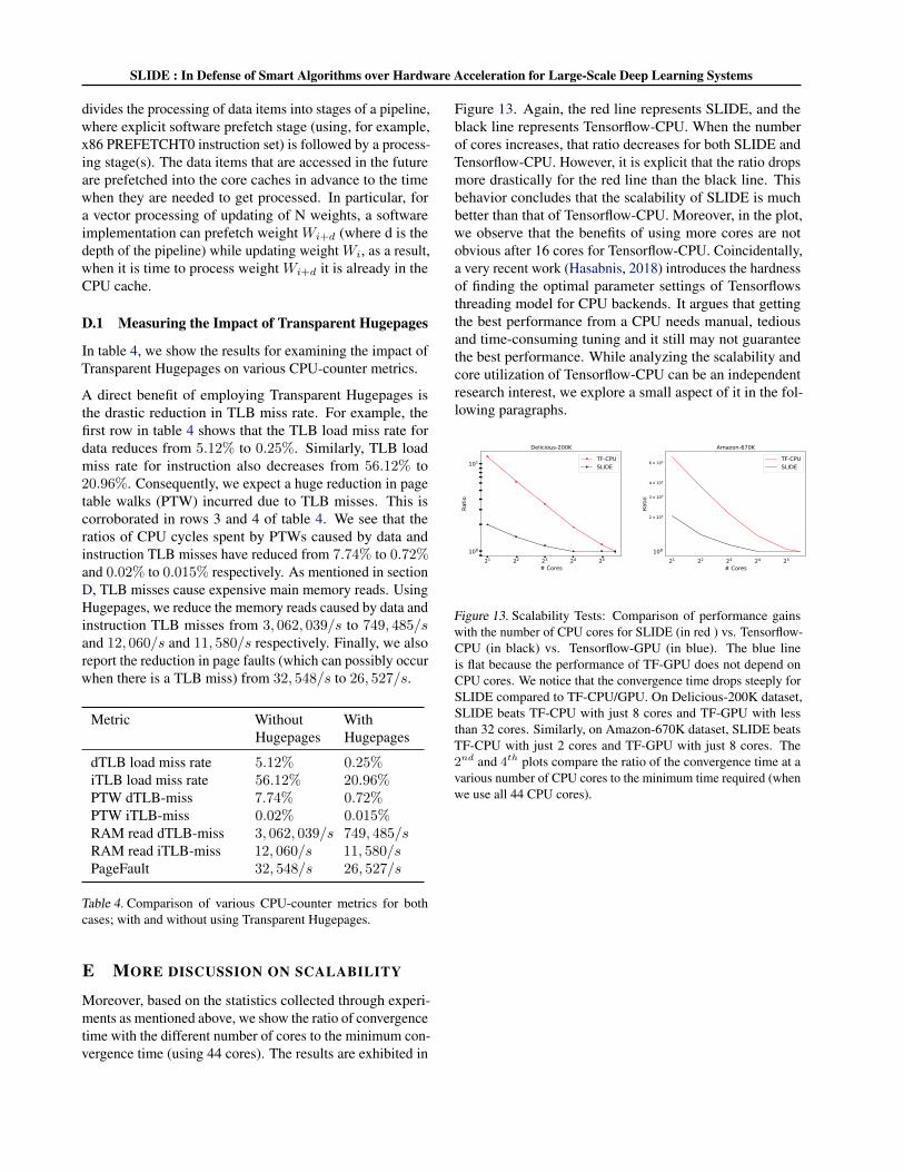
A direct benefit of employing Transparent Hugepages isthe drastic reduction in TLB miss rate. For example, thefirst row in table 4 shows that the TLB load miss rate fordata reduces from 5.12% to 0.25%. Similarly, TLB loadmiss rate for instruction also decreases from 56.12% to20.96%. Consequently, we expect a huge reduction in pagetable walks (PTW) incurred due to TLB misses. This iscorroborated in rows 3 and 4 of table 4. We see that theratios of CPU cycles spent by PTWs caused by data andinstruction TLB misses have reduced from 7.74% to 0.72%and 0.02% to 0.015% respectively. As mentioned in sectionD, TLB misses cause expensive main memory reads. UsingHugepages, we reduce the memory reads caused by data andinstruction TLB misses from 3, 062, 039/s to 749, 485/sand 12, 060/s and 11, 580/s respectively. Finally, we alsoreport the reduction in page faults (which can possibly occurwhen there is a TLB miss) from 32, 548/s to 26, 527/s.

Metric WithoutHugepages

WithHugepages

dTLB load miss rate 5.12% 0.25%iTLB load miss rate 56.12% 20.96%PTW dTLB-miss 7.74% 0.72%PTW iTLB-miss 0.02% 0.015%RAM read dTLB-miss 3, 062, 039/s 749, 485/sRAM read iTLB-miss 12, 060/s 11, 580/sPageFault 32, 548/s 26, 527/s

Table 4. Comparison of various CPU-counter metrics for bothcases; with and without using Transparent Hugepages.

E MORE DISCUSSION ON SCALABILITY

Moreover, based on the statistics collected through experi-ments as mentioned above, we show the ratio of convergencetime with the different number of cores to the minimum con-vergence time (using 44 cores). The results are exhibited in

Figure 13. Again, the red line represents SLIDE, and theblack line represents Tensorflow-CPU. When the numberof cores increases, that ratio decreases for both SLIDE andTensorflow-CPU. However, it is explicit that the ratio dropsmore drastically for the red line than the black line. Thisbehavior concludes that the scalability of SLIDE is muchbetter than that of Tensorflow-CPU. Moreover, in the plot,we observe that the benefits of using more cores are notobvious after 16 cores for Tensorflow-CPU. Coincidentally,a very recent work (Hasabnis, 2018) introduces the hardnessof finding the optimal parameter settings of Tensorflowsthreading model for CPU backends. It argues that gettingthe best performance from a CPU needs manual, tediousand time-consuming tuning and it still may not guaranteethe best performance. While analyzing the scalability andcore utilization of Tensorflow-CPU can be an independentresearch interest, we explore a small aspect of it in the fol-lowing paragraphs.

21 22 23 24 25

# Cores

100

101Ra

tio

Delicious-200KTF-CPUSLIDE

21 22 23 24 25

# Cores

100

2 × 100

3 × 100

4 × 100

6 × 100

Ratio

Amazon-670KTF-CPUSLIDE

Figure 13. Scalability Tests: Comparison of performance gainswith the number of CPU cores for SLIDE (in red ) vs. Tensorflow-CPU (in black) vs. Tensorflow-GPU (in blue). The blue lineis flat because the performance of TF-GPU does not depend onCPU cores. We notice that the convergence time drops steeply forSLIDE compared to TF-CPU/GPU. On Delicious-200K dataset,SLIDE beats TF-CPU with just 8 cores and TF-GPU with lessthan 32 cores. Similarly, on Amazon-670K dataset, SLIDE beatsTF-CPU with just 2 cores and TF-GPU with just 8 cores. The2nd and 4th plots compare the ratio of the convergence time at avarious number of CPU cores to the minimum time required (whenwe use all 44 CPU cores).

slide : in defense of smart algorithms over hardware ...as143/papers/slide_mlsys.pdfslide : in...

Documents