sliding mode control of a three-dof robotic system driven

Scientific Technical Review, 2015,Vol.65,No.1,pp.3-14 3

UDK: 527.93:519.713:007.52 COSATI: 12-01, 06-04

Sliding Mode Control of a Three-DOF Robotic System Driven by DC Motors

Mihailo Lazarević1) Srećko Batalov2)

This paper proposes a sliding mode control of a 3-DOF robotic system driven by DC motors. Primarily, a conventional sliding mode controller based on a PD sliding surface is designed. Numerical simulations have been carried out to show the proposed control system's robustness properties as well as the significance of the proposed control which resulted in reducing output oscillations (chattering-free) of the given robot. Finally, a simulation example shows the feasibility and effectiveness of the proposed approach.

Key words: robots, robotic system, theory of control, sliding mode control, nonlinear system.

1) University of Belgrade, Faculty of Mechanical Engineering, Department of Mechanics, Kraljice Marije 16, 11020 Belgrade 35, SERBIA 2) Energoprojekt Entel, Bulevar Mihaila Pupina 12, 11070 Belgrade, SERBIA Correspondence to: Mihailo Lazarević; e-mail: [email protected]

Introduction N recent years, the use of robotic systems in industrial and non-industrial applications has significantly been increased.

Due to highly coupled nonlinear and time varying dynamics, the robot motion tracking control is one of the challenging problems, [1-3]. Generally, nonlinear system model imprecision may come from an actual uncertainty about the plant (e.g., unknown plant parameters), or from the purposeful choice of a simplified representation of the system’s dynamics. Modeling inaccuracies can be classified into two major kinds: structured (or parametric) uncertainties and unstructured uncertainties (or unmodeled dynamics). The first kind corresponds to inaccuracies on the terms actually included in the model, while the second kind corresponds to inaccuracies on the system order. Modeling inaccuracies can have strong adverse effects on nonlinear control systems, [4].

One of the most important approaches to dealing with model uncertainty is robust control. Robust design techniques are essential in any field of engineering design because the working and durability of their pieces of work is always jeopardized by mutable and unpredictable environments,[5,6]. There are several approaches in this direction, for example optimal control, H-infinity control, high gain feedback, variable structure, etc. [4,7,8]. One of the novel ideas in this field is sliding mode control (SMC), which is a subset of variable structure control, [8,9]. Variable structure control (VSC) with sliding mode control was first proposed and elaborated in early 1950 in the USSR by Emelyanov and several co-researchers, [10-12]. In their pioneer works, the plant considered was a linear second-order system modeled in a phase variable form. Since then, VSC has developed into a general design method for a wide spectrum of system types including nonlinear systems, MIMO systems, discrete time models, and large scale and infinite dimensional systems,[13-15]. The most distinguished feature of VSC is its ability to result in very robust control systems. Loosely speaking, the term “invariant” means that the system is completely

insensitive to parametric uncertainty and external disturbances.

The SMC is a very popular strategy for the control of nonlinear uncertain systems, with a very large frame of application fields [5-8]. The sliding mode control methodology is one such robust control technique which has its roots in relay control. SMC has many attractive features such as invariance to matched uncertainties, model order reduction, simplicity in design, robustness against perturbations and some others [9,16,17].

One of the most intriguing aspects of the sliding mode is the discontinuous nature of the control action whose primary function is to switch between two distinctively different structures about some predefined manifold (sliding surface), such that a new type of system motion called a sliding mode exists in a manifold. The sliding mode contains two phases a) reaching phase in which the system states are driven from

any initial state to reach the switching manifolds (the anticipated sliding modes) in finite time, and

b) sliding phase in which the system is induced into the sliding motion on the switching manifolds, i.e., the switching manifolds become attractors. After sliding has been achieved, the system dynamics

matches that of the sliding surface. The robustness and the order reduction property of the sliding mode control come into picture only after the occurrence of the sliding mode. Due to the use of the discontinuous function, its main features are the robustness of the closed-loop system and the finite-time convergence. However, its design requires the knowledge of the bound on the uncertainties, which could be, from a practical point of view, a hard task: it often follows that this bound is overestimated, which yields excessive gain.

While, in theory, infinitely fast switching can provide asymptotically perfect tracking, in practice it implies a trade-off between tracking performance and control signal chatter, which is either undesirable due to noise considerations or impossible to achieve with real actuators.

I

4 LAZAREVIĆ,M.,BATALOV,S.: SLIDING MODE CONTROL OF A THREE-DOF ROBOTIC SYSTEM DRIVEN BY DC MOTORS

So, the main drawback of the sliding mode control, the well-known chattering phenomenon (for its analysis, see [18,19]) is important and could damage actuators and systems. Chattering is undesirable in the control of mechanical systems, since it causes an excessive control action leading to increased wear on the actuators and to excitation of the high order nonmodeled dynamics. Consequently, the demanded performance cannot be achieved, or even worse – the mechanical parts of the servo system can be destroyed. Therefore, chattering must be eliminated from the SMC system. Since chattering is caused by the discontinuous control, there exist several techniques to reduce a high switching amplitude, [20]. The first way to reduce chattering is the use of a boundary layer: in this case, many approaches have proposed adequate controller gains tuning [6]. The second way to decrease the effect of the chattering phenomenon is the use of a higher order sliding mode controller [21-23]. However, in both these control approaches, the knowledge of the bound on the uncertainties is required.

On the other hand, studies on the control of chain-like mechanical systems have been a subject of intensive and profitable research over the last three decades. Robotic systems, as dynamically coupled non-linear MIMO systems, have attracted the attention of many control scientists and engineers. The control of robotic systems is vital due to a wide range of their applications because these systems are multi-input multi-output, nonlinear and uncertain. Consequently, it is difficult to design accurately mathematical models for multiple degrees of freedom robot manipulators. As a significant tool for performing dangerous tasks, military robot systems can replace people in work in dangerous zones, so the controller designing military robot systems has become the focus in the field of automation. During the control process of robot systems, the presence of disturbances, model uncertainties, and nonlinear model parts is inevitable [24,25].

In addition, uncertainty in the parameters of both mechanical parts of robotic systems and actuating systems would cause more complexity. Therefore, strong mathematical tools are used in new control methodologies to design a controller with acceptable performance. It is obvious that stability is the minimum requirement in any control system; however, the proof of stability is not trivial especially in the case of nonlinear systems. One of the best nonlinear robust controls of robot manipulators is a sliding mode controller.The main reason to select this controller in a wide range area is to have acceptable control performance and solve two most important challenging topics in control, namely stability and robustness [26-28]. Here, because of nonlinear dynamics in robot manipulators, SMC is developed to control a three DOF robotic system with DC motors.

Introduction to classical sliding mode control

Problem statement The control of robot manipulators using the sliding mode

technique has a rather long history. Here, we briefly outline the basic theoretical concepts of sliding mode control, as it is done in [16, 26,29] and then the principle of the synthesis of control, firstly for SISO systems, then for MIMO systems.

First we define the sliding surface for a system defined by

( ), ( ) 0( ), ( ) 0

f x s xx =f x s x

+

−⎧ >⎨ <⎩

(1)

we say that the sliding surface is the set of all x such that

( ) 0s x = , and the functions ( )f x+ and ( )f x− tend towards that surface, for some x from its neighborhood, wherein the valid

( ) ( )( ) 0, ( ) 0,s x s xf x f xx x+ −∂ ∂< >

∂ ∂ (2)

Mathematically, ( )s x is often defined with

( ) [ ] ( )1 2 ... ... 0

Tnns x p p p x x x⎡ ⎤= =⎣ ⎦ (3)

where ip coefficients of the surface and dx x x= − is the deviation or as follows, [26]:

( ) ( )( )10, 0

nds x xdt λ λ−

= + = > (4)

The requirement that ( )f x+ and ( )f x− tend towards the surface ( ) 0s x = is crucial because it means that the trajectories of the system from the environmental surfaces in its "pooled", when the sliding mode occurs and the setpoint continues to move along the hypersurface with an infinite oscillating frequency and an infinitely small amplitude, while in the opposite trajectories of the system passed through the surface, without keeping on it. The following figures illustrate well how to modify the value of the function ( )f x near and on the sliding surface, as well as where the sliding mode occurs:

Figure 1. Value of the function f (.) in the neighborhood, and on the sliding surface.

Figure 2. Illustration when in systemsthe sliding operating mode occurs.

In a general case, the control algorithm in which a sliding operating mode appears, can be written in the form

( ) ( ), 0( ), 0

u x s(x)u xu x s(x)

+

−⎧ >= ⎨ <⎩

. (5)

A condition that generally appears in sliding regime it given as

0 0

lim 0, lim 0.s s

s s− +→ →

> < (6)

LAZAREVIĆ,M.,BATALOV,S.: SLIDING MODE CONTROL OF A THREE-DOF ROBOTIC SYSTEM DRIVEN BY DC MOTORS 5

When the system finds itself in a sliding operating mode, the question is how to describe its motions when the pre-defined control is undetermined on a hyperplane. Sliding dynamics can be described by introducing an equivalent control- fictitional continuous control that keeps the motion of the system on the sliding surface. Let us consider the nonlinear system described by:

( ) ( )x f x g x u= + (7)

From the condition of staying on the sliding surface

( ) ( )0, 0s x s x= = (8)

we can easily obtain the equivalent control and sliding dynamics

( ) ( ) ( ) ( ) ( )1

eqs x s x

u x g x f xx x

−∂ ∂⎛ ⎞= −⎜ ⎟∂ ∂⎝ ⎠ (9)

( ) ( ) ( ) ( ) ( )1s x s x

x I g x g x f xx x

−⎡ ⎤∂ ∂⎛ ⎞= −⎢ ⎥⎜ ⎟∂ ∂⎝ ⎠⎢ ⎥⎣ ⎦ (10)

Theoretically, in the ideal case, switching from ( ) 0u x+ =

to ( ) 0u x− = and vice versa takes place with an infinite frequency so that the actual behavior of the system is similar to the behavior of the system for the case when, instead of the proposed control, equivalent continuous control is used.

The object has greater time constants than the time constants of the correctional device, and higher harmonics, which appear in the slide operating mode, which arise from the discontinuous action of the relay, and which do not have a significant impact on the behavior of the whole system of automatic control, while the lower harmonics of the correctional device have only an impact on the behavior of the object and these harmonics are in fact equivalent control.

The dynamic characteristics of the system in the sliding operating mode depend on the position of the sliding hyperplane, and the desired behavior can be obtained by a suitable choice of the coefficients hypersurface. Besides the problem of describing the system in the sliding operating mode, a special problem is how to design a control system the states of which are led to the sliding hypersurface, possibly for the final time for each initial state. Generally, there are two main approaches to the synthesis of the sliding mode control. The first is that the control law consists only of the discontinuous control

( ) ( ) ( )1 sgnu x k x x= − (11)

and the second approach is that the proposed control is separated to the continuous and discontinuous part of the control,

( ) ( ) ( )2 sgnequ x u k x x= − (12)

Of course, there are other algorithms of the sliding mode control; as an example, we consider the algorithm which is introduced by [30]

( ) ( ) ( )3 4s k ( )equ x u k x x sgn x= − − (13)

But, here, we will explain the main idea in the case of the first two control laws. We have already mentioned that the sliding mode control has a discontinuous nature, and on the sliding plane there are infinitely fast changes of the control

signal. In practice, these oscillations have the final frequency as well as the limited accuracy of the calculation function

( ) 0s x = , which leads to an undesirable effect called chattering- oscillation output signals as well as problems to physically realize such control by the actuator.

The complete elimination of this phenomenon can be achieved by approximating the discontinuous function ( )sgn x with the symmetric saturation function sat(x) or the hyperbolic tangent tanh(x) .

/ ,

sgn( ) sgn(s),s s

x sε ε

ε<⎧≈ ⎨ >⎩

(14)

sgn( )x tanh(ks)≈ (15)

whose similarity with the function sgn( )x can be seen in the following Figures 3,4 for 1,0.5,0.1ε = and 1, 2,10k = .

-5 -4 -3 -2 -1 0 1 2 3 4 5

-1

-0.8

-0.6

-0.4

-0.2

0

0.2

0.4

0.6

0.8

1

t

sign

(t),

sat

(t/ ε

)

Figure 3. Saturation function ( )sat x

-5 -4 -3 -2 -1 0 1 2 3 4 5

-1

-0.8

-0.6

-0.4

-0.2

0

0.2

0.4

0.6

0.8

1

t

sign

(t),

tan

h(k*

t)

Figure 4. Function hyperbolic tangent tanh( )x

Mathematical model of a three DOF robotic system with DC motors

A robotic system is considered as an open linkage consisting of 1n + rigid bodies [ ]iV interconnected by n one-degree-of–freedom joints forming kinematical pairs of the fifth class, Fig.5, where the robotic system possesses n degrees of freedom. Here, the Rodriguez` method [31], is proposed for modeling the kinematics and dynamics of the


robotic system. The configuration of the robot mechanical model can be defined by the vector of the joint (internal) generalized coordinates q of the dimension ,n

( )q =(q1,q2,…,qn)T, with the relative angles of rotation (in the case of revolute joints) and relative displacements (in the case of prismatic joints). The geometry of the system has been defined by the unit vectors , 1,2,..., ,..,ie i j n= where the unit vectors ie describe the axis of rotation (translation) of the i -th segment with respect to the previous segment as well as the position vectors iρ and iiρ usually expressed in local

coordinate systems connected with the bodies ( ) ( )( ) ( ),i ii iiρ ρ .

The parameters , 1i iiξ ξ ξ= − denote the parameters for

recognizing the joints , 1i iiξ ξ ξ= − , 1iξ = -prismatic, 0-revolute. For the entire determination of this mechanical system, it is necessary to specify the masses im and the tensors of inertia CiJ expressed in local coordinate systems. In order that the kinematics of the robotic system may be described, the points ,i iO O′ are noticed somewhere at the axis of the corresponding joint ( )i such that they coincide in the reference configuration. The point iO is immobile with respect to the ( 1i − )-th segment and iO′ does so with respect to the i − th one; obviously, for a revolute joint ( )i , the points

iO and iO′ will coincide all the time during robotic motion. For example, the position vector of the end-effector Hr can be written as a multiplication of the matrices of transformation [ ]1,j jA − , the vectors iiρ and i

i iq eξ ,and it is expressed by

( )

[ ] ( ) ( )( )1

( ) ( )1,

1 1

( )n

iH ii i i

iin

i iij j iii i

i j

r q q e

A q e

ρ ξ

ρ ξ

=

−= =

= + =

⎛ ⎞⎜ ⎟= +⎜ ⎟⎝ ⎠

∑

∑∏ (16)

where the appropriate Rodriguez’ matrices of transformation are

[ ] [ ] ( ) ( )2( ) ( )1, 1 cos sind j d jj j

j j j jA I e q e q− ⎡ ⎤ ⎡ ⎤= + − +⎣ ⎦ ⎣ ⎦ (17)

and

( ) ( )( ) ( )0

, , , 00

j jTj d j

j j j j jj j

j j

e ee e e e e e e

e e

ζ η

ξ η ζ ζ ξ

η ξ

−⎡ ⎤⎢ ⎥⎡ ⎤= = −⎣ ⎦ ⎢ ⎥−⎣ ⎦

(18)

It is also shown [31], regardless of the chosen theoretical approach, that we could start from different theoretical aspects (e.g. general theorems of dynamic, d`Alembert`s principle, Langrange`s equation of the second kind, Appell`s equations, etc.) and get the equations of motion of the robotic system which can be expressed in the identical covariant form as follows

,1 1 1

( ) ( )

1,2,..., .

n n n

i i ia q q q q q Q

i n

βα αα αβ

α α β= = =

+ Γ =

=

∑ ∑∑ (19)

The kinetic energy of the given robotic system is given by

( ) [ ]( )1 1

1 1 ,2 2, 1,2,..., ,

n nT

kE a q q q a q

n

α βαβ αβ

α β

α β= =

= =

=

∑∑ (20)

where the coefficients aαβ are the covariant coordinates of

the basic metric tensor [ ] n na Rαβ×∈ and ,αβ γΓ

, , 1, 2,...,nα β γ = presents Christoffel symbols of the first kind defined as:

,12

aa a

q q qαγβγ αβ

αβ γ α β γ

∂∂ ∂⎛ ⎞Γ = + −⎜ ⎟⎜ ⎟∂ ∂ ∂⎝ ⎠

(21)

The generalized forces iQ can be presented in the

following expression (22) where , , , ,gc w ai i ii iQ Q Q Q Qβ denote

the generalized spring forces, gravitational forces, viscous forces, semi-dry friction and generalized control forces, respectively.

, ,...,gc w ai i i ii iQ Q Q Q Q Q i 1,2 nβ= + + + + = (22)

Figure 5. Open-chain structure of a robotic multi-body system

Fig.6 shows the equivalent circuit of a DC motor represented.

Figure 6. The equivalent circuit of a DC motor

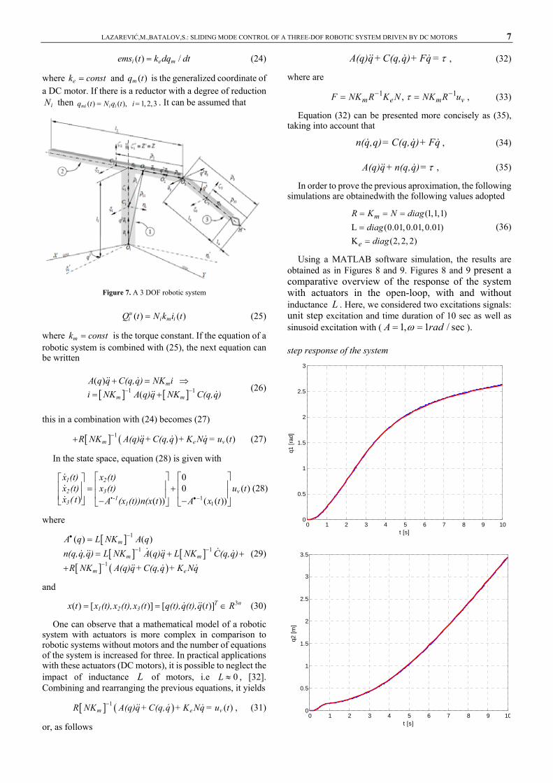
In this paper, we considered a robotic system with three degrees of freedom, see Fig. 7. The next equation describes the given circuit

( )( ) ( ) ( ), 1, 2,3ii i i i vi

di tR i t L ems t u t idt+ + = = (23)

where iR , iL , ii and viu are resistance, inductivity, electrical current and voltage, respectively. The electromotive force is


( ) /i e mems t k dq dt= (24)

where ek const= and ( )mq t is the generalized coordinate of a DC motor. If there is a reductor with a degree of reduction

iN then ( ) ( ), 1, 2,3mi i iq t N q t i= = . It can be assumed that

Figure 7. A 3 DOF robotic system

( ) ( )ui i m iQ t N k i t= (25)

where mk const= is the torque constant. If the equation of a robotic system is combined with (25), the next equation can be written

[ ] [ ]1 1

( )(

m

m m

A q q C(q,q) NK ii NK A q)q NK C(q,q)− −

+ = ⇒= +

(26)

this in a combination with (24) becomes (27)

[ ] ( )1 ( )m e vR NK A(q)q+C(q,q + K Nq = u t−+ (27)

In the state space, equation (28) is given with

1

1

00 ( )

) ( )) ( ( ))

1 2

2 3 v•-1

3 1

x (t) x (t)x (t) x (t) u tx ( t A (x (t))n(x t A x t•−

⎡ ⎤ ⎡ ⎤⎡ ⎤⎢ ⎥ ⎢ ⎥⎢ ⎥ = +⎢ ⎥ ⎢ ⎥⎢ ⎥ − −⎣ ⎦ ⎣ ⎦ ⎣ ⎦

(28)

where

[ ][ ] [ ]

[ ] ( )

1

1 1

1

( ) ( )(

m

m m

m e

A q L NK A qn(q,q,q) L NK A q)q L NK C(q,q)

R NK A(q)q+C(q,q + K Nq

−•

− −

−

=

= + +

+

(29)

and

3( ) [ )] [ ( )]T n1 2 3x t x (t),x (t),x (t q(t),q(t),q t R= = ∈ (30)

One can observe that a mathematical model of a robotic system with actuators is more complex in comparison to robotic systems without motors and the number of equations of the system is increased for three. In practical applications with these actuators (DC motors), it is possible to neglect the impact of inductance L of motors, i.e 0L ≈ , [32]. Combining and rearranging the previous equations, it yields

[ ] ( )1 ( )m e vR NK A(q)q +C(q,q + K Nq = u t− , (31)

or, as follows

A(q)q +C(q,q)+ Fq =τ , (32)

where are

1 1,m e m vF NK R K N NK R uτ− −= = , (33)

Equation (32) can be presented more concisely as (35), taking into account that

n(q,q)= C(q,q)+ Fq , (34)

A(q)q + n(q,q)=τ , (35)

In order to prove the previous aproximation, the following simulations are obtainedwith the following values adopted

(1,1,1)

L (0.01, 0.01, 0.01)K (2, 2, 2)

m

e

R K N diagdiag

diag

= = =

==

(36)

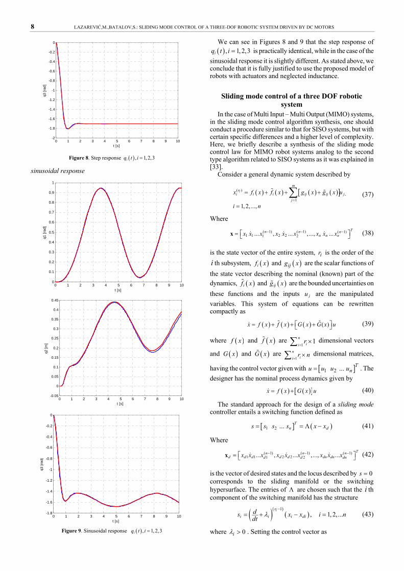
Using a MATLAB software simulation, the results are obtained as in Figures 8 and 9. Figures 8 and 9 present a comparative overview of the response of the system with actuators in the open-loop, with and without inductance L . Here, we considered two excitations signals: unit step excitation and time duration of 10 sec as well as sinusoid excitation with ( 1, 1 / secA radω= = ).

step response of the system

0 1 2 3 4 5 6 7 8 9 100

0.5

1

1.5

2

2.5

3

t [s]

q1 [

rad]

0 1 2 3 4 5 6 7 8 9 100

0.5

1

1.5

2

2.5

3

3.5

q2 [

m]

t [s]


0 1 2 3 4 5 6 7 8 9 10-2

-1.8

-1.6

-1.4

-1.2

-1

-0.8

-0.6

-0.4

-0.2

0

t [s]

q3 [

rad]

Figure 8. Step response ( ) , 1, 2,3iq t i =

sinusoidal response

0 1 2 3 4 5 6 7 8 9 100

0.1

0.2

0.3

0.4

0.5

0.6

0.7

0.8

0.9

1

t [s]

q1 [

rad]

0 1 2 3 4 5 6 7 8 9 10-0.05

0

0.05

0.1

0.15

0.2

0.25

0.3

0.35

0.4

0.45

t [s]

q2 [

m]

0 1 2 3 4 5 6 7 8 9 10-1.8

-1.6

-1.4

-1.2

-1

-0.8

-0.6

-0.4

-0.2

0

t [s]

q3 [

rad]

Figure 9. Sinusoidal response ( ) , 1, 2,3iq t i =

We can see in Figures 8 and 9 that the step response of ( ) , 1, 2,3iq t i = is practically identical, while in the case of the

sinusoidal response it is slightly different. As stated above, we conclude that it is fully justified to use the proposed model of robots with actuators and neglected inductance.

Sliding mode control of a three DOF robotic system

In the case of Multi Input – Multi Output (MIMO) systems, in the sliding mode control algorithm synthesis, one should conduct a procedure similar to that for SISO systems, but with certain specific differences and a higher level of complexity. Here, we briefly describe a synthesis of the sliding mode control law for MIMO robot systems analog to the second type algorithm related to SISO systems as it was explained in [33].

Consider a general dynamic system described by

( ) ( ) ( ) ( )[ ]( ),

1

1, 2,...,

im

ri i ij ij ji

j

x f x f x g x g x u

i n=

= + + +

=

∑ (37)

Where

( 1) ( 1) ( 1)1 1 2 21 2... , ... , ..., ...

Tn n nn n nx x x x x x x x x− − −⎡ ⎤= ⎣ ⎦x (38)

is the state vector of the entire system, ir is the order of the i th subsystem, ( )if x and ( )ijg x are the scalar functions of the state vector describing the nominal (known) part of the dynamics, ( )if x and ( )ijg x are the bounded uncertainties on these functions and the inputs ju are the manipulated variables. This system of equations can be rewritten compactly as

( ) ( ) ( ) ( )x f x f x G x G x u⎡ ⎤= + + +⎣ ⎦ (39)

where ( )f x and ( )f x are 1

1nii

r=

×∑ dimensional vectors

and ( )G x and ( )G x are 1

nii

r n=

×∑ dimensional matrices,

having the control vector given with [ ]1 2 ... Tnu u u u= . The

designer has the nominal process dynamics given by

( ) ( )[ ]x f x G x u= + (40)

The standard approach for the design of a sliding mode controller entails a switching function defined as

[ ] ( )1 2 ... Tn ds s s s x x= = Λ − (41)

Where

( 1) ( 1) ( 1)1 1 2 21 2... , ... ,..., ...

Tn n nd d d d d dn dnd d dnx x x x x x x x x− − −⎡ ⎤= ⎣ ⎦x (42)

is the vector of desired states and the locus described by 0s = corresponds to the sliding manifold or the switching hypersurface. The entries of Λ are chosen such that the i th component of the switching manifold has the structure

( )( )( )

1, 1, 2,...

ir

i i i dids x x i ndt λ

−= + − = (43)

where 0iλ > . Setting the control vector as


( )[ ] ( )[ ] ( )[ ] ( )1 1 sgndu G x f x x G x Q s− −= − Λ Λ − − Λ (44)

where Q is a positive-definite diagonal matrix chosen by the

designer provided that the inverse ( )[ ] 1G x −Λ exists. Choosing a the Lyapunov function candidate as

( ) 12

TV s s s= (45)

we get the equality

( ) ( )[ ] ( )sgn(s) ds PQ P I x f x f x= − + − Λ − − Λ (46)

with ( )( ) 1:P G G G −= Λ + Λ which is very close to the identity

matrix. If one sets SMCU u= then the system enters the sliding mode after a reaching phase. The expression in (43) can be interpreted as follows: - If there are no uncertainties, parameter perturbations, i.e.

when 0f = and 0G = , then (s)s Qsgn= − , and 0Ts s < is satisfied for any positive-definite Q . In this case, P I= and this result is straightforward.

- If only 0G = we obtain ( )sgn(s)s Q f x= − + Λ and

0Ts s < is satisfied if Q is a positive-definite diagonal matrix and the i th entry in the diagonal of Q is greater

than the supremum value of the i th row of fΛ . In this

case, P I= , too. - In the most general case, where neither 0f = nor 0G = ,

the expression in (43) is obtained. In this case, depending on the uncertainties influencing the input gains ( G ), the

matrix P is very close to the identity matrix, and utilizing the uncertainty bounds, the matrix Q can be chosen such

that the sign of s is preserved and 0Ts s < is satisfied. It could be therefore concluded that in the case of MIMO

systems, with an appropriate choice of the matrix Q , 0Ts s < can be obtained for 0s > and this result indicates that the error vector defined by the difference dx x− is attracted by the subspace characterized by 0s = and moves towards the origin according to what is prescribed by 0s = .

The motion during 0≠s is called the reaching mode, whereas the motion when 0s = is called the sliding mode. During the latter, dynamic mode, the closed loop system exhibits certain degrees of robustness against the modeling uncertainties; yet, the system is sensitive to noise as the sign of a quantity that is very close to zero determines the control action heavily. It is straightforward to show that a hitting time for the i -th subsystem satisfies the inequality

(0) /di i iit s Q≤ .

Example of the application of the sliding mode control law on a given robotic system

Here we present the results of the application of a recently considered algorithm (44). The robotic system in the necessary form can be described as

( ) ( ) ( )[ ] ( )1 10

,, ( )q

f x G xA q C q q Fq A q− −⎡ ⎤ ⎡ ⎤= =⎢ ⎥ ⎢ ⎥− + ⎣ ⎦⎣ ⎦

(47)

where T T Tx q q⎡ ⎤= ⎣ ⎦ is adopted for the state vector and the block diagram for the considered system becomes [34,35].

Figure 10. Block diagram for a sliding mode control system – classic approach Choosing the λ parameters of a sliding surface, we can

adjust (tune) the system performance in the sliding mode, as well as the hitting time (speed of convergence).

Although arbitrarily large values of λ are allowed, application practice is much different since the actuator presence causes some constraints on a possible choice of parameters. The best practice shows that above some critical λ values, the system response becomes much worse.

The conducted experiments on the perturbed system dynamic model resulted in the maximum values of

1 28, 3λ λ= = , and 3 3λ = , provided that the system keeps the desired response characteristics. It is decided to set the following values of parameters 1 2 35, 3, 3λ λ λ= = = , (48)

to achieve a higher degree of robustness against the parameter perturbations and modeling uncertainties. Taking the most general case where 0f ≠ and 0G ≠ , we vary (perturb) model parameters from 5% to 50% depending on real values expectations, and obtain the following estimation (close approximation) for the required matrix Q (done in MATLAB by an appropriate software code)

(50.8917 51.4562 61.1698)Q diag= (49)

Moreover, it is chosen to set Q as

(100 100 100)Q diag= (50)

to be able to compensate the maximum parameter


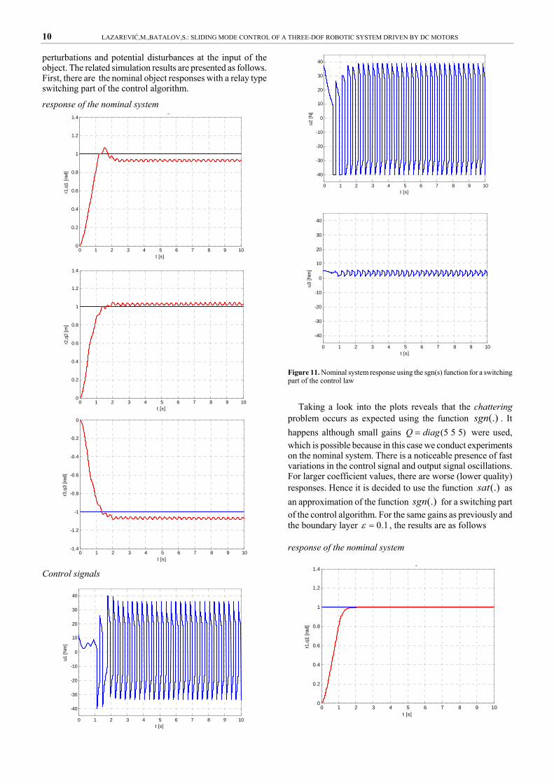
perturbations and potential disturbances at the input of the object. The related simulation results are presented as follows. First, there are the nominal object responses with a relay type switching part of the control algorithm.

response of the nominal system

0 1 2 3 4 5 6 7 8 9 100

0.2

0.4

0.6

0.8

1

1.2

1.4

r1,q

1 [r

ad]

t [s]

g

0 1 2 3 4 5 6 7 8 9 100

0.2

0.4

0.6

0.8

1

1.2

1.4

r2,q

2 [m

]

t [s]

0 1 2 3 4 5 6 7 8 9 10-1.4

-1.2

-1

-0.8

-0.6

-0.4

-0.2

0

t [s]

r3,q

3 [r

ad]

Control signals

0 1 2 3 4 5 6 7 8 9 10

-40

-30

-20

-10

0

10

20

30

40

t [s]

u1 [

Nm

]

0 1 2 3 4 5 6 7 8 9 10

-40

-30

-20

-10

0

10

20

30

40

t [s]

u2 [

N]

0 1 2 3 4 5 6 7 8 9 10

-40

-30

-20

-10

0

10

20

30

40

t [s]

u3 [

Nm

]

Figure 11. Nominal system response using the sgn(s) function for a switching part of the control law

Taking a look into the plots reveals that the chattering problem occurs as expected using the function (.)sgn . It happens although small gains (5 5 5)Q diag= were used, which is possible because in this case we conduct experiments on the nominal system. There is a noticeable presence of fast variations in the control signal and output signal oscillations. For larger coefficient values, there are worse (lower quality) responses. Hence it is decided to use the function (.)sat as an approximation of the function (.)sgn for a switching part of the control algorithm. For the same gains as previously and the boundary layer 0.1ε = , the results are as follows

response of the nominal system

0 1 2 3 4 5 6 7 8 9 100

0.2

0.4

0.6

0.8

1

1.2

1.4

r1,q

1 [r

ad]

t [s]

g


0 1 2 3 4 5 6 7 8 9 100

0.2

0.4

0.6

0.8

1

1.2

1.4r2

,q2

[m]

t [s]

0 1 2 3 4 5 6 7 8 9 10-1.4

-1.2

-1

-0.8

-0.6

-0.4

-0.2

0

t [s]

r3,q

3 [r

ad]

Control inputs

0 1 2 3 4 5 6 7 8 9 10-15

-10

-5

0

5

10

15

t [s]

u1 [

Nm

]

0 1 2 3 4 5 6 7 8 9 10-30

-20

-10

0

10

20

30

40

t [s]

u2 [

N]

0 1 2 3 4 5 6 7 8 9 103

3.5

4

4.5

5

5.5

t [s]

u3 [

Nm

]

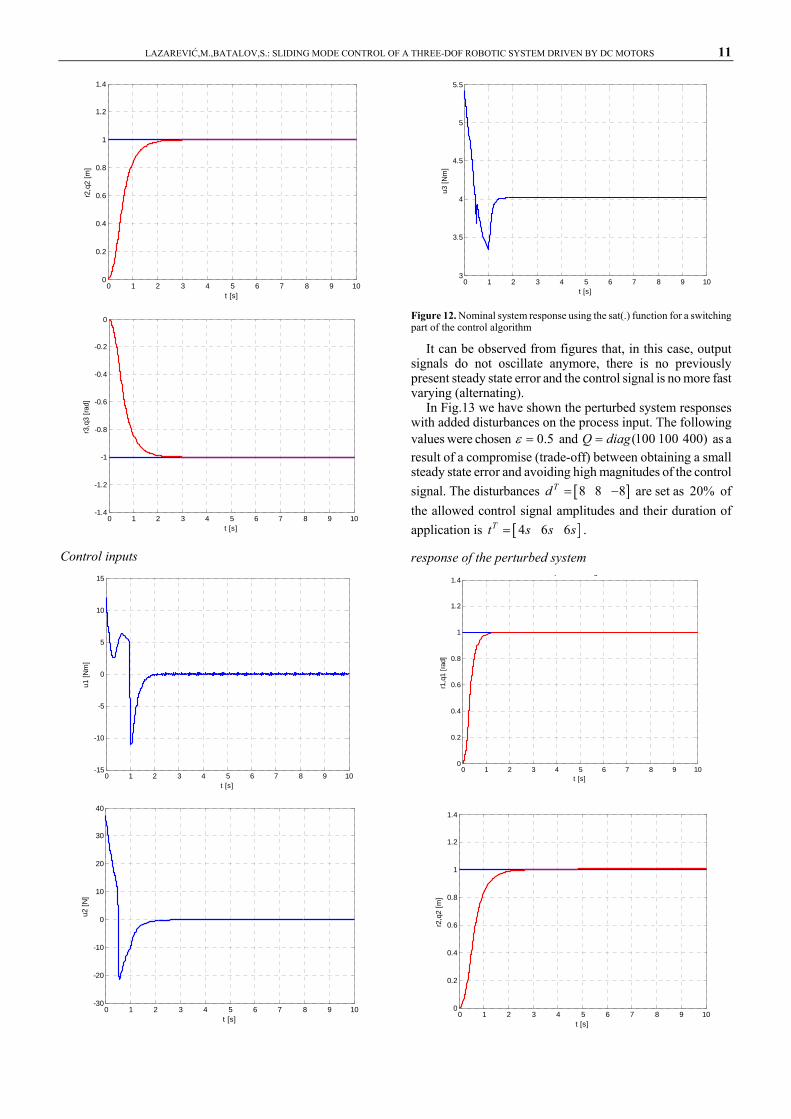
Figure 12. Nominal system response using the sat(.) function for a switching part of the control algorithm

It can be observed from figures that, in this case, output signals do not oscillate anymore, there is no previously present steady state error and the control signal is no more fast varying (alternating).

In Fig.13 we have shown the perturbed system responses with added disturbances on the process input. The following values were chosen 0.5ε = and (100 100 400)Q diag= as a result of a compromise (trade-off) between obtaining a small steady state error and avoiding high magnitudes of the control signal. The disturbances [ ]8 8 8Td = −

are set as 20% of

the allowed control signal amplitudes and their duration of application is [ ]4 6 6Tt s s s= .

response of the perturbed system

0 1 2 3 4 5 6 7 8 9 100

0.2

0.4

0.6

0.8

1

1.2

1.4

t [s]

r1,q

1 [r

ad]

p g

0 1 2 3 4 5 6 7 8 9 100

0.2

0.4

0.6

0.8

1

1.2

1.4

t [s]

r2,q

2 [m

]


0 1 2 3 4 5 6 7 8 9 10

-1.4

-1.2

-1

-0.8

-0.6

-0.4

-0.2

0

t [s]

r3,q

3 [r

ad]

Control inputs

0 1 2 3 4 5 6 7 8 9 10-40

-30

-20

-10

0

10

20

30

40

t [s]

u1 [

Nm

]

0 1 2 3 4 5 6 7 8 9 10-40

-30

-20

-10

0

10

20

30

40

t [s]

u2 [

N]

0 1 2 3 4 5 6 7 8 9 10-40

-30

-20

-10

0

10

20

t [s]

u3 [

Nm

]

Figure 13. Perturbed system response in the presence of input disturbance

Considering the response graphics, it can be concluded that the transition phase quality is not degraded despite huge input disturbance and parameter perturbations. The steady state error of 1.5 permille of a desired value for the first output, 8 permille for the second and 16 for the third are considerably decreased comparing to the PD control law of the feedback lineralized system (see [34]). It can be observed also that the control signals have certain oscillations which could not be avoided providing that the accuracy requirement is still satisfied.

Finally, we present the results of the reference tracking task. The reference is of a sinusoidal type and the system again perturbed with the presence of input disturbances of the same type as a desired value but with an amplitude of 10% of the maximum control signal magnitude, and a frequency of

5 /rad sω = five times bigger than the frequency of the reference signal.

The chosen controller parameters are 0.2ε = and (50 50 100)Q diag= .

response of the perturbed system in the presence of distrubance

0 1 2 3 4 5 6 7 8 9 10

-1

-0.8

-0.6

-0.4

-0.2

0

0.2

0.4

0.6

0.8

1

t [s]

r1,q

1 [r

ad]

0 1 2 3 4 5 6 7 8 9 10

-1

-0.8

-0.6

-0.4

-0.2

0

0.2

0.4

0.6

0.8

1

t [s]

r2,q

2 [m

]

0 1 2 3 4 5 6 7 8 9 10

-1

-0.8

-0.6

-0.4

-0.2

0

0.2

0.4

0.6

0.8

1

t [s]

r3,q

3 [r

ad]


Control inputs

0 1 2 3 4 5 6 7 8 9 10-20

-10

0

10

20

30

40

t [s]

u1 [

Nm

]

0 1 2 3 4 5 6 7 8 9 10-20

-10

0

10

20

30

40

t [s]

u2 [

N]

0 1 2 3 4 5 6 7 8 9 105

10

15

20

25

30

35

40

t [s]

u3 [

Nm

]

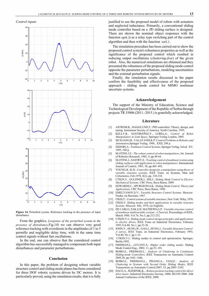
Figure 14. Perturbed system. Reference tracking in the presence of input disturbance

From the graphics, (response of the perturbed system in the presence of distrubance,Fig.14) we can observe very good reference tracking with overshoots in the amplitudes of 1 to 5 permille and negligible delay time, with in the same time control signals without fast oscillations.

In the end, one can observe that the considered control algorithm has successfully managed to compensate both input disturbances and parameter perturbations.

Conclusion In this paper, the problem of designing robust variable

structure control and sliding mode planes has been considered for three DOF robotic systems driven by DC motors. It is particularly proved, using the simulation results, that it is fully

justified to use the proposed model of robots with actuators and neglected inductance. Primarily, a conventional sliding mode controller based on a PD sliding surface is designed. There are shown the nominal object responses with the function sgn(.)) as a relay type switching part of the control algorithm and then with the function (.)sat .

The simulation procedure has been carried out to show the proposed control system's robustness properties as well as the significance of the proposed control which resulted in reducing output oscillations (chattering-free) of the given robot. Also, the numerical simulations are obtained and they presented the robustness of the proposed sliding mode control opposite the parameter perturbations, modeling uncertainties and the external perturbation signals.

Finally, the simulation results discussed in the paper confirm the feasibility and effectiveness of the proposed approach - sliding mode control for MIMO nonlinear uncertain systems.

Acknowledgement The support of the Ministry of Education, Science and

Technological Development of the Republic of Serbia through projects TR 35006 (2011.-2015.) is gratefully acknowledged.

Literature [1] ASTROM,K., HAGGLUND,T.: PID controllers: Theory, design, and

tuning. Instrument Society of America, North Carolina, 1995. [2] KELLY,R., SANTIBÁÑEZ,V., LORÍA,A.: Control of Robot

Manipulators in Joint Space, Springer-Verlag London, 2005. [3] SICILIANO,B., VALAVANIS,K.P: Control Problems in Robotics and

Automation,Springer Verlag, 1998,. XXII, 298 p. [4] ISIDORI,A.: Nonlinear Control Systems, Springer Verlag, 3rd ed. XV,

1995, 549 p. [5] SLOTINE,J.E.: The robust control of robot manipulators, Int. Journal

of Robotics Research, 1985, 4, pp.49-64. [6] SLOTINE,J., SASTRY,S.: Tracking control of nonlinear system using

sliding surfaces with application to robot manipulators. International Journal of Control, 1983, 38, pp.465–492.

[7] YOUNG,K.-K.D.: Controller design for a manipulator using theory of variable structure systems, IEEE Trans. on Systems, Man and Cybernetics, Feb.1978, 8(2), pp. 210-218.

[8] UTKIN,V., GULDNER,J., SHI,J.: Sliding Mode Control in Electro-Mechanical Systems. CRC Press, Boca Raton, 2009.

[9] EDWARDS,C., SPURGEON,S.K.: Sliding Mode Control: Theory and Applications, CRC Press, Boca Raton, 1998.

[10] EMELYANOV,S.V.: Variable Structure Control Systems. Moscow: Nauka, (in Russian), 1967.

[11] ITKIS,Y.: Control systems of variable structures, New York: Wiley, 1976. [12] ITKIS,Y: Sliding modes and their applications in variable structure

Systems. Moscow: Mir, 1978, (in English). [13] DE CARLO, ZAK,S.H. MATHEWS,G.P.: Variable structure control

of nonlinear multivariable systems: A Tutorial, Proceedings of IEEE, March 1988, Vol.76, No.3, pp.212-232.

[14] UTKIN,V.I.: Sliding mode control design principles and applications to electric drives, IEEE Trans on Industrial Electronics, February 1993,Vol.40, No.1, pp.23-36.

[15] JOHN,Y., HUNG,W., GAO,J., HUNG.J.: Variable Structure Control: A survey, IEEE Trans. on Industrial Electronics, February 1993, Vol.40, No.1, pp.1-22.

[16] UTKIN,V.I.: Sliding modes in control and optimization. Springer, Berlin,1992.

[17] FRIDMAN,L., LEVANT,A.: Higher order sliding modes. Sliding Mode Control Eng., 2002, 11, pp.53–101.

[18] BOIKO,I., FRIDMAN,L.: Analysis of Chattering in Continuous Sliding-mode Controllers, IEEE Transaction on Automatic Control 2005,50, pp.1442–1446.

[19] BOIKO,I., FRIDMAN,L., PISANO,A., USAI,E.: Analysis of Chattering in Systems with Second Order Sliding Modes, IEEE Transactions on Automatic Control,2007, 52, pp.2085–2102.

[20] HACE,A., JEZERNIK,K.,: Robust position tracking control for direct drive motor, Industrial Electronics Society, 2000. IECON 2000. 26th Annual Conference of the IEEE, 2000.


[21] LEVANT,A.: Sliding Order and Sliding Accuracy in Sliding Mode Control. International Journal of Control,2007, 58, pp.1247–1263.

[22] LEVANT,A.: Universal SISO Sliding-mode Controllers with Finite-time Convergence. IEEE Transactions on Automatic Control, 2001, 49, pp.1447–1451.

[23] LEVANT,A.: Principles of 2-sliding Mode Design. Automatica, 2007, 43, pp.576–586.

[24] CHEN,L., LIU,Y.: The robust control scheme for free-floating space manipulator to track the desired trajectory in jointspace, Acta Mechanica Solida Sinica, 2001, Vol.14, No.2, pp.183-188.

[25] EVANS,L.: Canadian space robotics on board the international space station,̍ 2005 CCToMM Symposium on Mechanisms, Machines, and Mechatronics. Canadian Space Agency, Montreal, Canada, May 26- 27, 2005.

[26] SLOTINE, J.J.E.,LI.W., Applied nonlinear control. Prentice-Hall Inc.1991.

[27] UTKIN,I.V.: Sliding mode in control optimization. New York: Springer-Verlag, 1992.

[28] IORDANOV, H.N.,SURGENOR,B.,W.: Experimental evaluation of the robustness of discrete sliding mode control versus linear quadratic control. IEEE Trans. On control System Technology, 2007, 5 (2),pp. 254-260.

[29] KHALIL,K.H.: Nonlinear Systems, Prentice-Hall, New Jersey, 2002. [30] PERRUQUETTI,W., BARBOT,J.P.: Sliding Mode Control in

Engineering, Marcel Dekker, 2008. [31] ČOVIĆ,V., LAZAREVIĆ,M.: Mechanics of Robots, Faculty of

Mechanical Engineering, University of Belgrade, (in Serbian), 2009. [32] LAZAREVIĆ,M,: Fractional Order Control of a Robot System Driven

by DC Motors, Scientific Technical Review, ISSN 1820-0206, 2012, Vol.62, No.2, pp.20-29.

[33] MEHMET,Ö.E., KASNAKOGLU,C.: A fractional adaptation law for sliding mode control, Int. J. Adapt. Control Signal Process., John Wiley & Sons, 2008.

[34] BATALOV,S.: Nonlinear robust control of a multivariable robotic system with the application of Fractional Calculus and genetic algorithms, Master work, Faculty of Mech. Eng. Belgrade, 2011, (in Serbian).

[35] PETROVIĆ,T., RAKIĆ,A.: Nonlinear systems, lectures, Faculty of Electrical Engineering, Belgrade, (in Serbian), 2011.

Received: 16.12.2014. Accepted: 10.02.2015.

Upravljanje u režimu klizanja kretanjem robotskog sistema sa tri stepena slobode pogonjen jednosmernim motorima

U ovom radu, predloženo je upravljanje u kliznom režimu kretanjem robotskog sistema sa 3 stepena slobode pogonjen jednosmernim motorima. Prvenstveno je projektovan kontroler u kliznom režimu i koji je baziran na PD kliznoj površi. Numeričke simulacije su sprovedene sa ciljem ilustrovanja osobina robusnosti predloženog sistema upravljanja kao i značaja smanjenja izlaznih oscilacija chattering-free datog robotskog sistema. Konačno, simulacioni primer pokazuje izvodljivost i efikasnost predloženog pristupa.

Ključne reči: roboti, robotizovani sistem, teorija upravljanja, upravljanje u režimu klizanja, nelinearni sistem.

Управление в скользящем режиме движением роботизированной системы с тремя степенями свободы с приводом двигателями

постоянного тока В данной работе предлагается, чтобы управлять в скользящем режиме движением роботизированной системы с 3 степенями свободы с приводом двигателями постоянного тока. Это в первую очередь значит, что предназначен контроллер в скользящем режиме и он основан на ПД поверхности скольжения. Численное моделирование проводилось для иллюстрации надёжности характеристик предлагаемой системы управления, а также и важности сокращения выходных колебаний chattering-free данной роботизированной системы. Наконец, пример моделирования показывает целесообразность и эффективность предложенного подхода.

Ключевые слова: роботы, роботизированная система, теория управления, управление в скользящем режиме, нелинейная система.

Contrôle dans le régime de glissement chez le système robotique à trois degrés de liberté propulsé par les moteurs à courant continu

Dans ce papier on propose le contrôle dans le régime de glissement chez le système robotique à trois degrés de liberté propulsé par les moteurs à courant continu. On a conçu principalement le contrôleur dans le régime de glissement qui est basé sur la surface glissante PD. Les simulations numériques ont été réalisées dans le but d’illustrer les propriétés de robustesse chez le système proposé de contrôle ainsi que pour la signification des réductions des oscillations sortantes «chattering-free» du système robotique donné. Finalement l’exemple de simulation démontre la faisabilité et l’efficacité de l’approche proposée.

Mots clés: robots, système robotisé, théorie de contrôle, contrôle dans le régime de glissement, système non linéaire.

sliding mode control of a three-dof robotic system driven

Documents