Sloshing and scaling: experimental study in a wave canal at two different scales

O. Kimmoun (1)

, A. Ratouis (2)

, L. Brosset (2)

(1)Ecole Centrale Marseille

Marseille, France (2)Liquid motion dept, Gaztransport & Technigaz

Saint-Rémy-lès-Chevreuse, France

ABSTRACT

Sloshing model tests are the basis of any sloshing assessment for a new

membrane LNG carrier project. The statistical pressure results have to

be scaled to full scale in order to derive design loads. The approach for

scaling is not obvious as multi-physics occur within the impacts.

Experimental modeling is based on the Froude scaling assumption: if

the forced motions at small scale are defined with a geometrical scale

1/λ and a time scale 1/√λ, the velocities in both fluids, liquid and gas,

should be in Froude accordance at both scales. This is exact for the

global flow but Braeunig et al., (2009) have shown that it is wrong

locally during the sloshing impacts, even though the density ratio

between the fluids are kept the same at both scales, because the speeds

of sound in the model liquid and gas are not in Froude accordance with

the speeds of sound of respectively LNG and natural gas. The study

presented here is an experimental attempt to show evidence of this so-

called compressibility bias of sloshing experimental modeling.

Performing sloshing tests with model tanks at two different scales

would have led only to a statistical comparison of the impact pressures.

In order to have a direct deterministic comparison of Froude-similar

liquid impacts on a wall at two different scales, the study deals with

single breaking waves in a laboratory wave canal at two different scales

referred to as scales s1 and s1/2.

After describing the experimental set-up and the breaking wave

generation process, the paper shows the difficulties to reproduce

accurately local developments of the impacts and the significant

consequences of light discrepancies on the pressures. At the end the

study describes how a relatively good similarity between flows at the

two scales is obtained. A global analysis shows the general trend of the

scaling for the pressures inside gas pockets.

KEY WORDS: Sloshing, Liquid Impact, Breaking Waves, Flume

tank, Experiments, scaling, Froude, Compressibility, LNG carriers

INTRODUCTION

Repeating sloshing model tests leads to a large scattering of the impact

pressures in the sample. Only after a statistical post-processing of long

duration tests, allowing for a large sample, will the pressure results

become reasonably repeatable. The origin of the scattering of impact

pressure is commonly attributed to local phenomena while the global

flow is considered as quasi-deterministically defined. The scattering

which is also a lack of repeatability can be attributed to the complex

turbulent and three-dimensional flows. It makes sense that studying a

single two-dimensional breaking wave should lead to a better

repeatability. Reproducing two flows at two different geometrical

scales consists in imposing Froude-scaled excitations to a liquid.

According to waves equations the global flow (velocities) remains the

same after Froude-scaling. What happens locally around each impact

area (the local flow), during a very short duration starting with the

compression of the escaping gas, is more complex and involves multi-

physics including gas compressibility effects. For realistic impacts, the

physics local phenomena should occur with the same intensity at both

scales. The transfer of momentum between gas and liquid is one of the

phenomena and is governed by the ratio of densities between gas and

liquid. Keeping the same density ratio at both scales takes off a bias

source between the scales. Thus, it allows for the studying of other

sources of differences. The principle remaining source of bias is then

compressibility effects. Other sources could be mentioned such as

phase transition or different hydro-elastic effects.

The objective of the study presented in this paper is to compare

deterministically local fluid impact pressures obtained experimentally

at two different scales for similar Froude-scaled global flows. This

objective leads directly to different pre-requirements:

1. Ensure that, at each scale, the global flow is repeatable when

repeating carefully the same wave maker signal

2. Ensure that, at each scale, local impact pressure measurements are

repeatable when repeating carefully the same global flow

3. Ensure that the experimental set-up allows a good similarity of the

global flows at the two scales for the different conditions studied

The paper explains which precautions are necessary to achieve these

requirements.

The experimental facility selected is the ~17 m laboratory flume tank

of Ecole Centrale Marseille (ECM) (Kimmoun et al., 2009). A flap-

type wave maker generates idealized, unidirectional breaking waves by

a focusing process. The waves focus at a selected distance of the flap

and impact an instrumented rigid wall when breaking.

TEST SET-UP AND BREAKING WAVE GENERATION

Two scales are studied with a geometrical ratio of ½ in all directions.

They are referred to as scale s1 and s1/2. Thanks to a movable test wall,

the set-up is adapted for dealing with the two scales. At both scales, the

distances between the wave maker and the wall, the liquid heights in

the canal, the locations of the pressure sensors with regards to the free

surface at rest are geometrically scaled and the wave maker signals are

both geometrically and time scaled in order to be in a Froude

similarity. Only the size and the density of the pressure sensors on the

wall remain the same at both scales.

Flume tank

The wave tank is 16.77 m long. A rotational wave maker is installed at

an end. At the other end the instrumented wall is located at D1 = 15.5 m

from the flap at scale s1 and at D1/2 = 7.75 m at scale s1/2. The

longitudinal walls are transparent sections of glass supported by

metallic frames. The movable flap and a horizontal bottom lay above

the fix concrete floor of the room. Figure 1 and Figure 2 show

schematically the installation and the main dimensions at both scales.

Fig.1 - Schematic description of the wave canal at both scales

During the whole study, except a specific sensitivity study on the water

depth, the water depth at rest was fixed to h1 = 0.7 m at scale s1 and

h1/2 = 0.35 m at scale s1/2.

Instrumentation

Four resistive wave gauges referred to as wg1, wg2, wg3, wg4 are

installed in the first part of the canal. The distances from the wave

maker are given in table 1.

Table 1 – distance from the flap to the wave gauges at both scales

wg1 (m) wg2 (m) wg3 (m) wg4 (m)

Scale s1 1.65 13.1 13.45 13.85

Scale s1/2 0.825 6.55 6.725 6.925

Two capacitive wire sticks

are glued on the movable

test wall in order to

measure accurately the

run-up of the waves along

the wall after impacting.

Their location on both

sides of the wall is shown

in Figure 2.

Fig.2 – Locations of run-up wave

gauges and laser sheet for PIV

88 PCB pressure transducers are screwed in two metallic modules

inserted in the wall. The PCB sensors are piezo-electric. They have

a sensitive circular area of 5.5 mm diameter.

The same two metallic modules are used at both scales enabling

setting a hundred sensors. The two modules are identical. Their

positions on the test wall at both scales with regards to the water

free surface at rest are shown in Figure 3. The sensors are mainly

arranged on horizontal and vertical lines. The minimum distance

between two sensors on these lines is 1 cm. In the main area of

interest (close to the impact zone), the lines of sensors have been

doubled in a staggered way so that, assuming the flow is perfectly

2D, a measurement every 5 mm in both directions is possible. A

zoom-in in Figure 3 shows this sensor arrangement.

The data acquisition is performed by a National Instruments PXI

system with a sampling frequency at 40 kHz

Fig.3 – Test wall and metallic modules for the fixation of the pressure

sensors at scale s1 and scale s1/2

A high speed camera (Vision Research Phantom 7.3) is installed

close to the wall in order to look closely at the impact area through

the longitudinal glass wall. The camera enables a resolution of

800 x 600 pixels² at a frequency up to 6800 fps.

Most of the time the high speed camera was used for a visualization

of the free surface impacting the wall. It was focused on a

longitudinal vertical plan enlighten by a continuous ion laser

(Spectra-physics 0.3 W / 458-514 nm) after a fluorescein solution

had been introduced into the water. In that case the high speed

video recording was in the range between 1000 and 4000 fps,

depending on the period of the test campaign.

For the most interesting cases, the conditions were repeated with a

Particle Image Velocimetry (PIV) measurement technique. A

continuous YAG laser (Spectra-physics 5 W / 532 nm) was used

and the water was seeded by 6 m diameter silver coated hollow

glass spheres with a density of 1.1 g/cm3. The image acquisition

frequency was set to 2000 fps in that case. This set-up corresponds

to a PIV technique adapted to continuous laser lighting instead of

pulsed laser lighting. It was previously used successfully for flow

visualizations of breaking solitons on a beach (Kimmoun et al.,

2009).

The acquisition of wave probe signals was synchronized with the

start of the wave maker. Video recording was synchronized with

the pressure data.

Wave maker and focalisation technique

The wave maker is moved by a hydraulic engine. The flap rotates

around a horizontal axis located 40 cm under the raised bottom of the

tank.

A focusing technique is used to generate a targeted wave elevation

η(x, t) at given focal distance x of the flap and time t, from a wave

amplitude spectrum a(ω), ω being the rotation frequency. The flap

rotation signal θ(x, t) is deduced from the spectrum thanks to the

modified flap transfer function C(ω). (1)

The integration on ω is carried out by a discretization on about 65,000

equally spaced frequencies. Figure 4 shows a wave packet generated by

the flap using this focusing process.

The forced flap motions start with the small high frequency oscillations

and finish with the largest low frequency wave. All wave components

meet at the same time at the focal point, close to the wall, generating a

large breaking wave. The focal distance between the flap and the wall is

thus the main parameter to adjust the shape of the free surface just

before the impact.

Fig. 4 - Generation of a wave packet in ECM flume tank

When the focal point is far upstream the wall, the wave breaks before

the wall. This kind of impact generates very low pressures and is not of

much interest from a designer point of view. When the focal point is

chosen closer to the wall, impacts with an entrapped air pocket may

occur, referred to as air-pocket impacts. While the crest is breaking, the

interaction between the wave and the wall induces a trough run-up. The

air pocket is entrapped between the crest, the trough and the wall. The

size of the air pocket is getting smaller when the focal point is getting

closer to the wall. If the focal point is set further in the same direction,

even beyond the wall, the trough run-up becomes dominant with

regards to the crest momentum and no real impact occurs. This is

referred to as a slosh impact. In between these two usual situations,

there is a theoretical situation corresponding to an air pocket, the

volume of which is null. This case induces a much localized flip-

through of the free surface just in front of the wall. It is referred to as

flip-through impact. The closer the situation is to the flip-through,the

larger and sharper is the peak pressure.

These different kinds of waves have been studied in detail, in a larger

facility, in the frame of the Sloshel project. For more information refer

to Brosset et al., (2009). The Sloshel project was studying full scale

waves with the real NO96 containment system. The scales studied in

ECM must be considered for comparison purpose as scales s1=1/7.5

and s1/2=1/15.

Figure 5 shows four air-pocket impacts obtained at scale s1 for four

focal distances increasing progressively from 15.3 m to 15.6 m.

x = 15.30 m x = 15.40 m

x = 15.50 m x = 15.60 m

Fig. 5 - Breaking wave profiles just before impacting for four air-pocket

impacts corresponding to four close focal distances x at scale s1

The four snapshots are given in each case at a time just before the

impact. The different status in the wave breaking process is clearly

observed for the four different focal distances. The sooner the breaking;

the larger the air pockets.

The type of wave signals that were intended to be studied at first was

the signals derived by Froude-scaling from those studied during the

Sloshel project at a much larger scale. Some modifications, in order to

obtain a better repeatability of the results, have been applied to these

signals and are described later. The recent full scale test campaign of

Sloshel project that took place in April 2010 took advantage of these

improvements.

This study has been focused exclusively on the air-pocket impacts,

tuning the focal point location for obtaining different sizes of the air

pocket.

REPEATABILITY OF THE GLOBAL FLOW AT A GIVEN

SCALE

Without any caution, repetitions of the same wave maker signal may

lead to slightly different global flows, and hence different shapes of the

free surface just before impact. In that case the comparison of the

impact pressures would not make sense. Figure 6 shows three

repetitions of the same flap motion at scale s1/2. The waves generated

are referred to as 354, 355 and 356.

0 1 2 3 4 5

0

0.5

1

1.5

time (ms)

Pre

ssu

re (

ba

r)

354

355

356

Fig. 6 - Free surface profiles at the impact time for three different

waves obtained with the same theoretical wave maker motion (left) and

corresponding max pressure signals (right). Waves 354, 355 and 356

For different reasons, analysed later, the wave profiles (Figure 6 – left)

obtained with the same excitation of the flap are quite different.

Consequently, with no surprise, the impact pressure time traces

(Figure 6 – right), given each time at the sensor getting the maximum

pressure, are also significantly different.

For a relevant comparison of impact pressures after repetitions of the

same wave maker command, a pre-requirement is that the global flow

until the impact is the same. So, all measurements in the chain from the

wave generation to the wave impact described in Table 2 must be

precisely the same for the same theoretical signal of the wave maker.

Table 2 – chain of measurements from wave maker to wall to be

checked for repeatability studies

1 Wave maker motion

2 Wave elevations at wave gauges wg1, wg2, wg3, wg4

3 Wave surface profile at impact time

Only after fulfilling this pre-requirement of identical global flows, will

the impact pressures be compared.

Fixing, a priori, a minimum accuracy when comparing the wave

profiles at the impact time from high speed camera pictures, would be

artificial. The final comparison of the impact pressures will determine

this actual accuracy, which is required on the global flow. Nevertheless,

it is reasonable to consider, for instance from Figure 6, that the order of

magnitude is the millimetre.

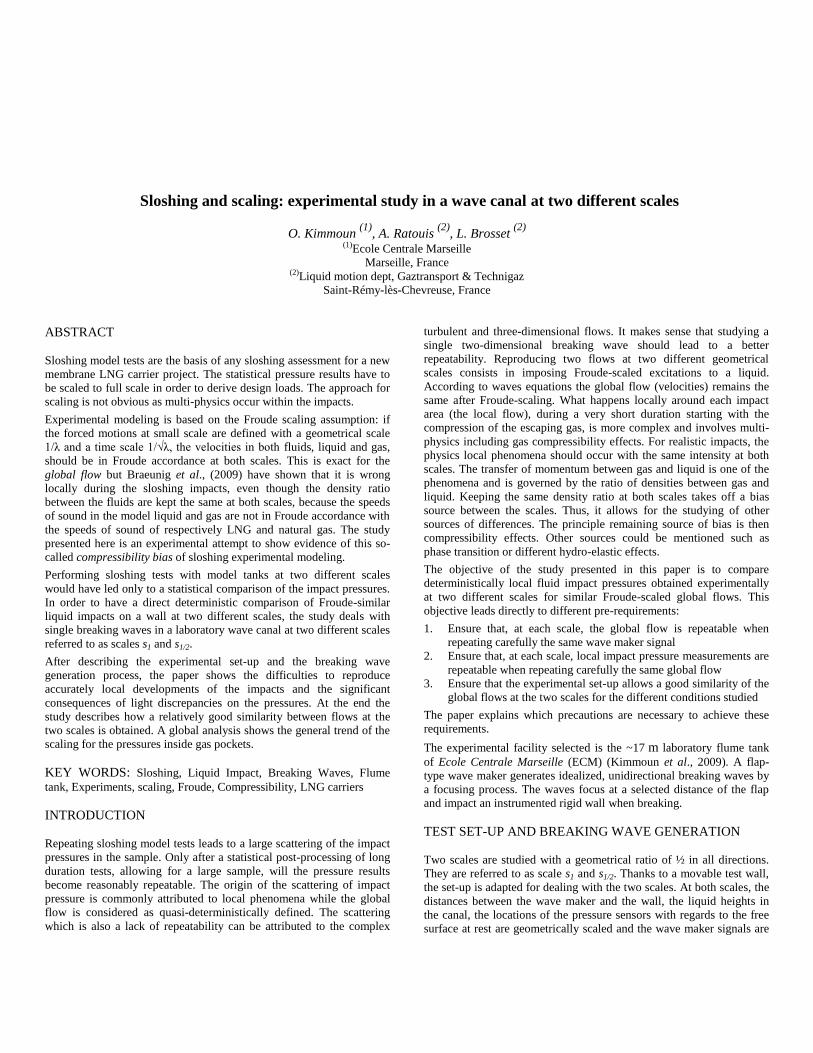
Two major sources have been identified as responsible of most of the

discrepancies observed in Figure 6:

The repeatability of the wave maker motions,

The uncertainty on the water depth measurement.

Repeatability of the wave maker motions

Repeatability of the wave maker motion for the same theoretical signal

is obviously a condition for a good repeatability of the future wave

development. Considering the accuracy required after the 15.5 m wave

traveling, an extreme accuracy is required on the flap signals.

Figure 7 shows the wave elevations, as measured by the closest wave

gauge to the wave flap (wave gauge wg1 on Table 1), for the three wave

repetitions shown in Figure 6 (waves 354, 355 and 356 at scale s1/2).

115 120 125

-4

-2

0

2

4

6

time (s)

ele

vatio

n (

cm)

354

355

356

Fig. 7 - Wave elevations from the wave gauge wg1 for the three waves

in Fig. 6 generated by the same theoretical wave maker signal.

Left: overview of the signal, Right: zoom-in on the highest crest

So, the discrepancies on the largest crest at wave gauge wg1 at only

0.825 m of the flap are already around 10 mm. In that condition, one

can obviously not reach the targeted accuracy of 1 mm at the wall level.

From the beginning of this study, it was believed that a main source of

non repeatability was the high frequency content of the wave spectrum

applied to the wave maker. Indeed the theoretical flap motion

amplitude spectrum a(ω)/C(ω), which is derived from the wave

amplitude spectrum a(ω) thanks to the transfer function of the flap

C(ω), has a high frequency content that will lead to very short duration

and short amplitude oscillations of the flap in time domain. The flap

may not be able to follow mechanically accurately these oscillations but

they have a theoretical influence on the wave profile at the wall level.

So a new wave spectrum was searched in order to replace the Sloshel

spectrum as(ω). The Ricker spectrum ar( ) commonly used in

geophysics was selected (Brinks, 2008):

(2)

with the pulsation. Four parameters (m, T, A, a) enable the

adjustment of the spectrum. The parameter a is used to determine the

peak of frequency p using:

(3)

Parameter A sets the amplitude, m and T are shape parameters of the

spectrum. These parameters were fitted in order to minimize the mean

quadratic difference with the Sloshel spectrum.

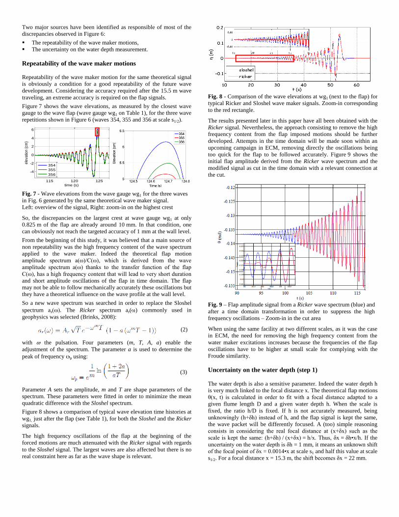
Figure 8 shows a comparison of typical wave elevation time histories at

wg1, just after the flap (see Table 1), for both the Sloshel and the Ricker

signals.

The high frequency oscillations of the flap at the beginning of the

forced motions are much attenuated with the Ricker signal with regards

to the Sloshel signal. The largest waves are also affected but there is no

real constraint here as far as the wave shape is relevant.

Fig. 8 - Comparison of the wave elevations at wg1 (next to the flap) for

typical Ricker and Sloshel wave maker signals. Zoom-in corresponding

to the red rectangle.

The results presented later in this paper have all been obtained with the

Ricker signal. Nevertheless, the approach consisting to remove the high

frequency content from the flap imposed motions should be further

developed. Attempts in the time domain will be made soon within an

upcoming campaign in ECM, removing directly the oscillations being

too quick for the flap to be followed accurately. Figure 9 shows the

initial flap amplitude derived from the Ricker wave spectrum and the

modified signal as cut in the time domain with a relevant connection at

the cut.

Fig. 9 – Flap amplitude signal from a Ricker wave spectrum (blue) and

after a time domain transformation in order to suppress the high

frequency oscillations – Zoom-in in the cut area

When using the same facility at two different scales, as it was the case

in ECM, the need for removing the high frequency content from the

water maker excitations increases because the frequencies of the flap

oscillations have to be higher at small scale for complying with the

Froude similarity.

Uncertainty on the water depth (step 1)

The water depth is also a sensitive parameter. Indeed the water depth h

is very much linked to the focal distance x. The theoretical flap motions

θ(x, t) is calculated in order to fit with a focal distance adapted to a

given flume length D and a given water depth h. When the scale is

fixed, the ratio h/D is fixed. If h is not accurately measured, being

unknowingly (h+δh) instead of h, and the flap signal is kept the same,

the wave packet will be differently focused. A (too) simple reasoning

consists in considering the real focal distance at (x+δx) such as the

scale is kept the same: (h+δh) / (x+δx) = h/x. Thus, δx = δh•x/h. If the

uncertainty on the water depth is δh = 1 mm, it means an unknown shift

of the focal point of δx = 0.0014•x at scale s1 and half this value at scale

s1/2. For a focal distance x = 15.3 m, the shift becomes δx = 22 mm.

The four snapshots of Figure 5 obtained for focal distances shifted

regularly of 10 cm gave an idea of what kind of wave profile

discrepancy could be expect with a 2 cm shift.

Figure 10 shows the wave profiles just before impact for four different

water depths increasing by step of 1 mm from 34.9 cm.

So, the uncertainty on the water depth is to be considered also as an

amplified uncertainty on the focal distance.

This influence is obviously especially important when working around

the focal distance corresponding to the flip-through area, as this

phenomenon is very sharp.

The water depth has another major influence on the ability for a given

network of sensors to capture phenomena that may induce strong

gradient of pressures over the distance between two consecutive

sensors. This particular issue is addressed in a next sub-section.

The water depth should thus be measured with a special care, when the

flume is totally at rest, which requires a long waiting time between tests

in order to ensure that the first mode of the tank is totally damped.

Fig. 10 - profiles of breaking waves just before impacting for four

different water depths and the same wave maker signal

A laboratory flume like ECM‟s is absolutely watertight: no leakage is

to be accounted for. Nevertheless the evaporation cannot be avoided

and leads to significant change of the water fill level over a day or a

night with regards to the accuracy targeted.

This phenomenon could explain the discrepancies that are observed

when comparing the last run of a day (e.g. run 354) and the first run of

the next day (e. g. run 355). The runs 354 and 355 selected in Figure 6

illustrate this evaporation consequence.

So, repeatability for a target focal distance must be performed over a

short period of time (a few hours) in order to avoid any tiny change of

water depth by evaporation.

Repeatability of the global flow (results)

When comparing repetitions of the Ricker signal in a short period of

time, a good repeatability of the global flow has been obtained at both

scales for different focal distances leading to repeatable different sizes

of gas-pocket impacts.

At scale s1/2, four tests carried out in a row, the same day as run 355 but

later have been selected. They correspond to a small gas pocket.

Figure 11 shows the four superimposed wave profiles just before

impact.

At scale s1, two tests (124 and 125), performed one after the other in a

short period of time, have been selected. They correspond to a small

gas-pocket impact.

-5 -4 -3 -2 -1 047

48

49

50

51

52

x (cm)

z (c

m)

356

357

358

359

Fig. 11 -. Wave profiles for four repetitions of the same flap signal. –

Scale s1/2

Figure 12 illustrate the good repeatability obtained on the wave

elevations time traces measured by the gauges wg3 and wg4 (see

Table 1). It can be observed that the signals superimpose very

accurately.

Figure 13 shows the pictures recorded by the high speed camera just

before the impact. A superimposition of the snapshots is presented. The

results match perfectly.

Fig. 12 - Wave elevation time traces at wg3 (left) and wg4 (right) for two

repetitions of the same wave maker signal at scale s1. Tests 124 and 125

Fig. 13 – High speed camera shots at 11ms (top) and 2ms before impact

(bottom) for two repetitions of the wave maker signal (same as in

Fig. 12. Run 124 (red) - Run 125 (blue) – overlaid (violet)

REPEATABILITY OF RELEVANT PRESSURE

MEASUREMENTS FOR SAME GLOBAL FLOWS

Assuming good repetitions of a global flow has been obtained at a

given scale, shown by accurate repetitions of the parameters of Table 2,

it might be relevant to compare the impact pressures. New difficulties

rise then, one has to be aware of.

Even restricted to the study of air-pocket impacts, unilateral wave

impacts in a flume are able to generate very sharp pressure loads both

in time and space in two different situations:

For large air pocket impacts at the crest level (crest impact of a

breaking wave).

For small air-pocket, a sharp flip of the free surface enables locally

a quick turn of the velocities from horizontal to vertical direction.

These sharp pressure peaks cannot be disregarded. Indeed Sloshel

project (see Bogaert, Léonard, Marhem, Leclère & Kaminski, 2010)

has shown, by means of full scale wave impact tests in a flume, that the

structure of the NO96 membrane containment system used for LNG

ships responds highly to such sharp pressure excitations.

This section describes how far the sharpness of these peak pressure

signals is captured in space by the network of sensors shown in

Figure 3 and in time by the acquisition sampling frequency.

Obviously, at the crest level for large air-pocket events or for small air-

pocket impacts, only when the sharp peak pressures are captured, is the

repeatability requirement relevant.

Large air-pocket impacts

For large air-pocket impacts, the crest hits first the wall leading to

localized sharp pressures. In that case, the momentum of the crest is not

overcome by the trough run-up.

Figure 14 shows the development of a gas pocket impact through

different snapshots separated by a time step of 5 ms. Impact of the crest

confines the air-pocket, which is compressed horizontally against the

wall by the liquid pushing behind, and vertically by the trough run-up.

Fig. 14 - Snapshots of a gas pocket impact at four instants: t = -10 ms,

-5 ms, 0 ms and 5 ms - Time aligned on max pressure at the crest level -

Scale s1

The pushing liquid and the stiffness of the gas pocket act in an

antagonist way very similar as a mass/spring system leading to

oscillations of the gas pocket. The pressure is uniform into the gas

pocket and two sensors completely entrapped in it measure exactly the

same pressure. The pressure evolution into the pocket is totally

determined by the evolution of its volume through the equation of state.

Figure 15 shows the pressure signature of such an impact, focusing on

the crest level located at around 99 cm above the bottom. The pressure

sensor at 99 cm captured a sharp peak pressure which corresponds to

the crest impact. After the decay of the sharp peak, the pressure in the

crest oscillates with the same frequency as seen by the pressure sensor

located 1 cm below, which is inside the pocket. The oscillation period

is around 8 ms. The sharp peak is captured by one sensor but not by the

sensors at 1 cm above or at 1 cm below. The gradient of pressures is,

thus, very high over a distance of 1 cm.

Vertical pressure profile evolution Pressure signals for 3 sensors close to

the crest

Fig. 15 – Pressure signature of an air-pocket impact at the crest level –

Scale s1

For all large air-pocket impacts, the crest impact is necessarily present.

However, there are some for which no sharp peak can be detected by

the pressure sensors. It means thus that the peak has not been captured,

it does not mean that it does not exist. In that case, only the air pocket

pressure is measured. The measurement may be more easily repeatable

but the fact remains that the pressure measurement is not relevant.

Small air-pocket impacts

Small air-pocket impacts behave differently than large ones. When

considering air-pocket impacts with progressively smaller pockets,

there is a threshold from which the trough run-up becomes dominant

with regards to the crest momentum. The free surface has to flip

sharply just in front of the wall. The horizontal momentum of the

pushing liquid behind the remaining pocket is thus abruptly

transformed to vertical momentum added to the trough run-up, which

becomes a violent vertical jet. The crest is not strong enough to prevent

this run-up development.

Figure 16 shows the evolution of a small air-pocket impact. Four

snapshots from the high-speed camera at instants separated by 5 ms are

given. The velocity fields as determined by the PIV technique, is

superimposed to the camera pictures.

Large velocities can be observed at the crest level just before the

impact. Maximum velocity recorded is 7 m/s. From the successive

locations of the trough and of the tip of the crest, it can be noticed that

the wave trough is accelerating and its vertical velocity becomes higher

than the horizontal velocity of the crest. Unfortunately the trough is in a

shadow area of the PIV.

Fig. 16 – Negative snapshots with velocity field of a small gas pocket

impact at four instants: t=-10 ms, -5 ms, 0 ms and 5 ms - Time aligned

on max pressure at the crest level - Scale s1 - Colour scale from light

blue to dark red. Dark red for the max velocity reported in each picture.

Figure 17 shows the pressure signature recorded by the sensors

in the impact area.

For this type of small gas-pocket impact, the pressure signature is very

different than for larger air-pocket impacts. The maximum pressure is

higher (here 6.3 bar) but is still restricted to a very small area. Over the

distance of 5 mm, the pressure decrease is about 4 bars.

Vertical pressure profile evolution Pressure signals for 3 sensors

close to the crest

Fig. 17 – Pressure signature of a small air-pocket impact – Scale s1.

There are still oscillations of the signal, but very quickly damped,

showing that a small fraction of gas remained entrapped. Consequently,

the frequency of the oscillations becomes very high (about 0.7 ms). The

time duration of the peak is around 0.25 ms. When studying small air-

pocket impacts, the volume of air pockets, hence the frequency of the

oscillations and the maximum impact pressures are very sensitive to

variations of the focal distance.

Table 3 shows the results of a sensitivity study at scale s1. The focal

distance varies from 15.57 m to 15.62 m with a minimum step of 1 cm.

The focal distance 15.62 m corresponds to a slosh impact. In that case

there is no gas pocket. For a variation of the focal distance of the order

of a centimeter, impact characteristics vary very sharply.

Table 3 - Sensitivity to the focal distances for small gas pockets

Focal (m) 15.57 15.59 15.60 15.62

width (cm) 7.63 3.29 1.62 No

Frequency (Hz) 160 440 1040 No

Pressure (bars) 1.80 5.41 6.45 1.55

Uncertainty on the water depth (step 2)

The uncertainty on the water depth determination has already been

addressed in the previous section for its influence on the global flow.

At the same time, considering the high gradient of pressures that can be

expected locally, the uncertainty on the fill level makes the relative

location of the sensors with regards to the highest pressure area

uncertain, bringing thus a new uncertainty on the pressure

measurement.

A short sensitivity study on the water depth has been carried out at

scale s1/2. Four runs have been performed for increasing depths from

34.9 cm to 35.2 cm by steps of 1 mm. As the variations on the water

depth are here considered as uncertainties, these differences are

normally unknown by the experimenter who would apply a nominal

signal to the wave maker. So, the wave maker signal is kept the same

for the different water depths studied. It corresponds to a focal distance

of 7.765 m. If the ratio of the focal distance to the depth is considered, a

3 mm variation on the depth corresponds to a 66 mm variation on the

focal distance.

Results are reported in Table 4 in terms of maximum width of the gas

pocket, frequency of its oscillations and maximum pressure on all

sensors.

Table 4 - Sensitivity study of the water depth for a given flap signal

– scale s1/2.

Depth (cm) 34.9 35.0 35.1 35.2

width (cm) 0.38 0.50 0.69 0.91

Frequency (Hz) 1125 930 870 570

Pressure (bar) 0.740 1.383 1.423 2.075

The profiles of the breaking waves just before impact have already been

shown in Figure 10.

The two different influences of the water depth are clearly seen in

Table 4. The influence on the global flow is observed through the width

of the air pocket and consequently through the frequency of its

oscillations. For decreasing widths of the pockets, the maximum

pressures should normally increase. Here the opposite trend is

observed, showing the second effect of the water depth change: the fit

of the pressure sensor location giving the maximum pressure is getting

progressively worse and worse with regard to the crest location when

passing from a water depth of 35.2 cm to 34.9 cm. However the bad

repetition of the global flow should not enable a comparison of the

pressures.

The quantity of dissolved air into the water plays also obviously a

role on the quality of the repetitions during the few days after refilling

the tank. During this period, the water is moved by the flap and by the

impacts, the amount of dissolved air decrease and reach a constant

value. No sensitivity study has been performed yet to quantify the

influence of this parameter but all tests have been performed with the

same water.

Technical ability to capture the sharp peak pressures

How far can the sharp peak pressures that occur at the crest of large air-

pocket impacts or for small air-pocket impacts be captured?

In space, it has been shown that the gradient of pressure can be very

large over a distance of 5 mm. The diameter of the sensors is 5.5 mm

and the staggered locations of the sensors every 5 mm enables to have

almost a continuum of pressure sensors in the vertical direction „(see

Figure 3). So, theoretically, even a sharp peak of pressure should, most

of the time, not be missed. Nevertheless, just a tiny change in the

location of the crest with regards to the sensor location should modify

much the measurement. If the pressure hot spot is covered by the area

with the two horizontal lines of sensors, it should not be missed.

In time, one can wonder whether the sampling frequency is sufficient

or not. Figure 18 shows zoom-ins of the maximum pressure area for the

signals obtained respectively in Figure 15 for large air-pocket impacts

at the crest level and in Figure 17 for small air-pocket impacts. The dots

represents the sampled times.

Large-pocket impact of Fig. 12

Sensor at 99 cm Small pocket impact of Fig. 14

Sensor at 99.5 cm

Fig. 18 – data acquisition sampling of the pressure signals at small and

at large air pocket impacts. - Sampling frequency f = 40 kHz – Scale s1

The sampling frequency of 40 kHz adopted for all tests enables to

discretize adequately the sharpest pressure signals obtained.

Repeatability of the pressure measurements at each scale

It has been shown that the high density of sensors used (distance

minimum of 5 mm) together with their rather large diameter (5.5 mm)

should enable to capture spatially the sharp pressure peaks obtained for

local crest impacts of large air-pocket events or for small air pocket

impacts. The maximum pressure recorded is an average on the sensor

diameter. As far as repeatability is concerned the governing parameter

is the accurate location of the pressure hot spot with regards to the

locations of the pressure sensors and especially to the two staggered

horizontal lines of sensors shown in Figure 3. So with an accuracy of

1 mm on the wave profile just before the impact at scale s1 (global

flow), and with repetitions in a short period of time (no change in the

water depth) good repeatability of the pressures is achievable.

Two examples are given corresponding to scales s1 and s1/2.

At scale s1/2 four tests performed during the same day have been

selected. They correspond to tests 356 to 359 that proved to have very

similar global flows (see Figure 11). Figure 19 shows the pressure time

traces obtained from the sensor recording the maximum pressure.

0 1 2 3 4 5

0

0.5

1

1.5

time (ms)

Pre

ssu

re (

ba

r)

356

357

358

359

Fig. 19 - Pressure traces at the same location for four repetitions of

the same flap signal. Wave profile before impact in Figure 11

These tests correspond to a small gas-pocket impact. The frequency of

the gas pocket oscillations is 700 Hz. The frequency range obtained

during the tests at scale s1/2 is between 225 Hz and 715 Hz. Therefore,

these tests correspond to a size of gas pocket close to the smallest

obtained during the tests at scale s1/2. A very good repeatability of the

pressure time traces was obtained.

At scale s1, two tests (124 and 125), performed also one after the other

in a short period of time, have been selected. They correspond also to a

small gas-pocket impact. The repeatability of the global flow has

already been shown in Figures 12 and 13. The repeatability of the

impact pressure measurement is illustrated in Figures 20 and 21.

Fig. 20 – Pressure time traces given by sensor n°55 for two repetitions

of the wave maker signal. Test 124 (blue), test 125 (red) – Scale s1

Figure 20 presents the pressure time traces obtained by a representative

sensor located in the high pressure area. Figure 21 shows the time

evolution of the pressure profile along the wall.

Fig. 21 – Time evolution of the pressure profile along the wall for two

repetitions of the wave maker signal. Test 124 (left), Test 125 (right) –

Scale s1

These two tests generated high pressures peaks. An accuracy of 3% was

nevertheless obtained on the repetition of the pressure peaks.

So, a good repeatability of the pressure peak measurements is

achievable. It requires challenging conditions:

a good repeatability of the wave maker motions that can be

facilitated by removing as far as possible the high frequency

content of the wave spectrum

a dense repartition of sensors in the hot spot area in order not to

miss very localized high pressure zones

no variation of the water depth, which requires to perform the tests

consecutively in a short period

During the whole test campaign covering almost 400 tests. At each

scale, only a few series fulfil all the requirements. Many waves have

been performed with a good repetition of the global flow but with a

pressure hot spot outside the dense covering of the sensor

configuration.

SIMILARITY AT BOTH SCALES

In the previous section, it has been shown that a good repeatability of

the pressure measurements can be achieved when challenging

precautions are fulfilled. Now, a second requirement for a deterministic

comparison of pressures at two different scales (see introduction) is a

good similarity of the global flows at the two scales for the different

conditions studied. According to the theory, the global flow should be

similar if the wave maker signals are Froude-scaled. So, the accurate

scaling of the flap signal is addressed in this section. Then the issue of

the pressure diameter scaling rises.

Wavemaker signal scaling

With the rotational wave maker there is a potential difficulty to apply

the Froude-scaling that is to be studied carefully for a good similarity of

global flows.

The scaling process for the flap signal can be described as follows:

The starting point is the Ricker spectrum ar(ω) and the transfer

function of the flap C(ω)

From these data are deduced the elevation of the free surface

η(x1, t1) and the rotation of the flap θ(x1, t1) at scale s1, where x1 is

the location of the focal point and t1 is the time (see formula (1))

By Froude-scaling the free surface elevation one obtains:

η1/2(x, t) = η(x1/2, t1/2) at scale s1/2

From η1/2 and the transfer function of the flap we deduce the

rotation signal of the flap at scale s1/2: θ1/2(x, t) = θ(x1/2, t1/2)

When applying directly this process, very similar waves are created at

both scales in terms of free surface elevation, as measured by the last

wave gauges wg4 before the wall (see Table 1). Nevertheless these

small discrepancies induce different free surface profiles just before the

impact and the comparison of the pressures at both scales in these

conditions is not relevant.

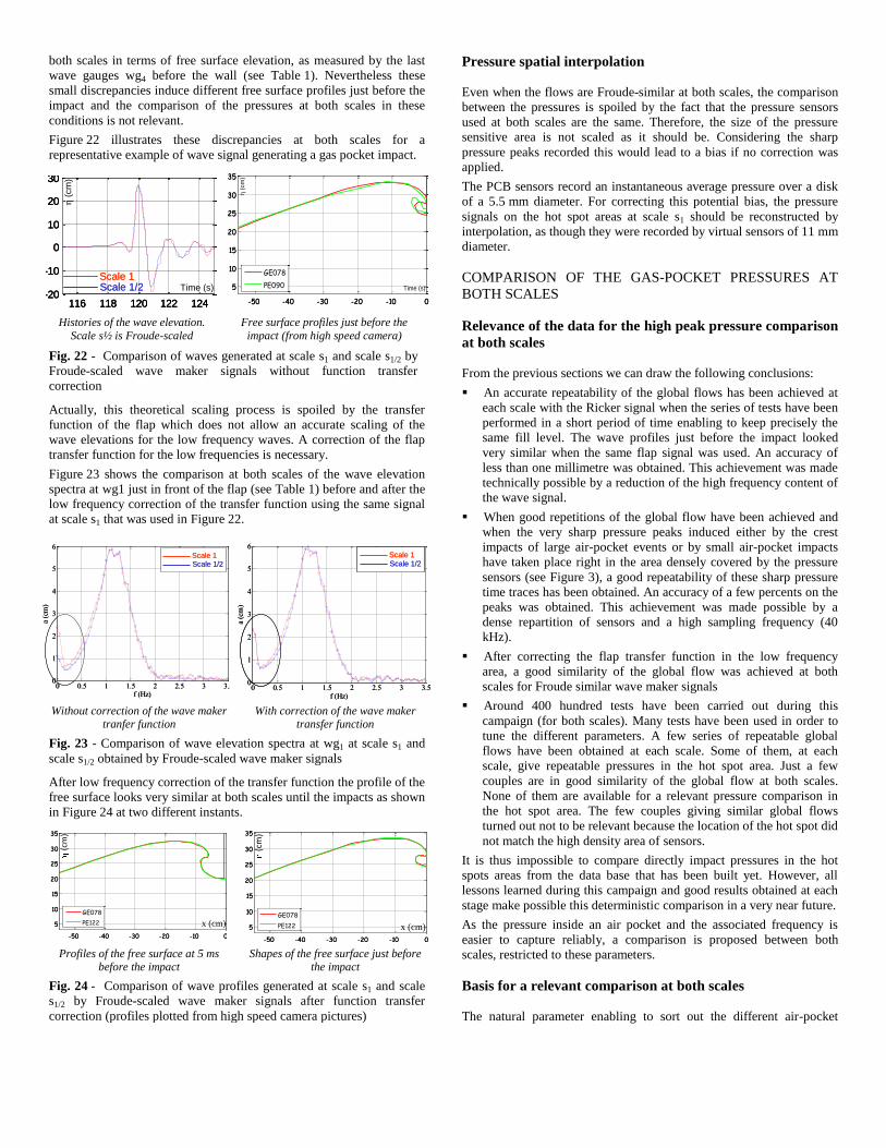
Figure 22 illustrates these discrepancies at both scales for a

representative example of wave signal generating a gas pocket impact.

Histories of the wave elevation.

Scale s½ is Froude-scaled

Free surface profiles just before the

impact (from high speed camera)

Fig. 22 - Comparison of waves generated at scale s1 and scale s1/2 by

Froude-scaled wave maker signals without function transfer

correction

Actually, this theoretical scaling process is spoiled by the transfer

function of the flap which does not allow an accurate scaling of the

wave elevations for the low frequency waves. A correction of the flap

transfer function for the low frequencies is necessary.

Figure 23 shows the comparison at both scales of the wave elevation

spectra at wg1 just in front of the flap (see Table 1) before and after the

low frequency correction of the transfer function using the same signal

at scale s1 that was used in Figure 22.

Without correction of the wave maker tranfer function

With correction of the wave maker transfer function

Fig. 23 - Comparison of wave elevation spectra at wg1 at scale s1 and

scale s1/2 obtained by Froude-scaled wave maker signals

After low frequency correction of the transfer function the profile of the

free surface looks very similar at both scales until the impacts as shown

in Figure 24 at two different instants.

Profiles of the free surface at 5 ms before the impact

Shapes of the free surface just before the impact

Fig. 24 - Comparison of wave profiles generated at scale s1 and scale

s1/2 by Froude-scaled wave maker signals after function transfer

correction (profiles plotted from high speed camera pictures)

Pressure spatial interpolation

Even when the flows are Froude-similar at both scales, the comparison

between the pressures is spoiled by the fact that the pressure sensors

used at both scales are the same. Therefore, the size of the pressure

sensitive area is not scaled as it should be. Considering the sharp

pressure peaks recorded this would lead to a bias if no correction was

applied.

The PCB sensors record an instantaneous average pressure over a disk

of a 5.5 mm diameter. For correcting this potential bias, the pressure

signals on the hot spot areas at scale s1 should be reconstructed by

interpolation, as though they were recorded by virtual sensors of 11 mm

diameter.

COMPARISON OF THE GAS-POCKET PRESSURES AT

BOTH SCALES

Relevance of the data for the high peak pressure comparison

at both scales

From the previous sections we can draw the following conclusions:

An accurate repeatability of the global flows has been achieved at

each scale with the Ricker signal when the series of tests have been

performed in a short period of time enabling to keep precisely the

same fill level. The wave profiles just before the impact looked

very similar when the same flap signal was used. An accuracy of

less than one millimetre was obtained. This achievement was made

technically possible by a reduction of the high frequency content of

the wave signal.

When good repetitions of the global flow have been achieved and

when the very sharp pressure peaks induced either by the crest

impacts of large air-pocket events or by small air-pocket impacts

have taken place right in the area densely covered by the pressure

sensors (see Figure 3), a good repeatability of these sharp pressure

time traces has been obtained. An accuracy of a few percents on the

peaks was obtained. This achievement was made possible by a

dense repartition of sensors and a high sampling frequency (40

kHz).

After correcting the flap transfer function in the low frequency

area, a good similarity of the global flow was achieved at both

scales for Froude similar wave maker signals

Around 400 hundred tests have been carried out during this

campaign (for both scales). Many tests have been used in order to

tune the different parameters. A few series of repeatable global

flows have been obtained at each scale. Some of them, at each

scale, give repeatable pressures in the hot spot area. Just a few

couples are in good similarity of the global flow at both scales.

None of them are available for a relevant pressure comparison in

the hot spot area. The few couples giving similar global flows

turned out not to be relevant because the location of the hot spot did

not match the high density area of sensors.

It is thus impossible to compare directly impact pressures in the hot

spots areas from the data base that has been built yet. However, all

lessons learned during this campaign and good results obtained at each

stage make possible this deterministic comparison in a very near future.

As the pressure inside an air pocket and the associated frequency is

easier to capture reliably, a comparison is proposed between both

scales, restricted to these parameters.

Basis for a relevant comparison at both scales

The natural parameter enabling to sort out the different air-pocket

116 118 120 122 124-20

-10

0

10

20

30

116 118 120 122 124-20

-10

0

10

20

30

116 118 120 122 124-20

-10

0

10

20

30

116 118 120 122 124-20

-10

0

10

20

30

Scale 1Scale 1/2 Time (s)

η(c

m)

116 118 120 122 124-20

-10

0

10

20

30

116 118 120 122 124-20

-10

0

10

20

30

116 118 120 122 124-20

-10

0

10

20

30

116 118 120 122 124-20

-10

0

10

20

30

Scale 1Scale 1/2

116 118 120 122 124-20

-10

0

10

20

30

116 118 120 122 124-20

-10

0

10

20

30

116 118 120 122 124-20

-10

0

10

20

30

116 118 120 122 124-20

-10

0

10

20

30

Scale 1Scale 1/2Scale 1Scale 1/2 Time (s)

η(c

m)

-50 -40 -30 -20 -10 0

5

10

15

20

25

30

35

x (cm)

(cm

)

GE078

PE090 Time (s)

η(c

m)

-50 -40 -30 -20 -10 0

5

10

15

20

25

30

35

x (cm)

(cm

)

GE078

PE090 Time (s)

η(c

m)

0 0.5 1 1.5 2 2.5 3 3.50

1

2

3

4

5

6

f (Hz)

a (c

m)

petite échelle

grande échelle

Scale 1Scale 1/2

0 0.5 1 1.5 2 2.5 3 3.50

1

2

3

4

5

6

f (Hz)

a (c

m)

petite échelle

grande échelle

Scale 1Scale 1/2Scale 1Scale 1/2

-50 -40 -30 -20 -10 0

5

10

15

20

25

30

35

x (cm)

(cm

)

GE078

PE122

(cm)

x (cm)

-50 -40 -30 -20 -10 0

5

10

15

20

25

30

35

x (cm)

(cm

)

GE078

PE122

(cm)

x (cm)

-50 -40 -30 -20 -10 0

5

10

15

20

25

30

35

x (cm)

(cm

)

GE078

PE122

(cm)

x (cm)

-50 -40 -30 -20 -10 0

5

10

15

20

25

30

35

x (cm)

(cm

)

GE078

PE122

(cm)

x (cm)

0 0.5 1 1.5 2 2.5 3 3.50

1

2

3

4

5

6

f (Hz)

a (c

m)

petite échelle

grande échelle

Scale 1Scale 1/2

0 0.5 1 1.5 2 2.5 3 3.50

1

2

3

4

5

6

f (Hz)

a (c

m)

petite échelle

grande échelle

Scale 1Scale 1/2Scale 1Scale 1/2Scale 1Scale 1/2

impacts at both scales should be the focal distance. However, it has

been shown how a small uncertainty on the water depth can lead to a

large uncertainty on the focal distance and more generally on the

Froude-similarity of the flap steering signals.

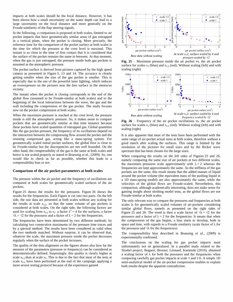
In the following, a comparison is proposed at both scales, limited to air

pocket impacts that have geometrically similar areas of gas entrapped

in a vertical plane, when the pocket is closing. More precisely, the

reference time for the comparison of the pocket surface at both scales is

the time for which the pressure at the crest level is maximal. This

instant is so close to the time of first contact that it is considered that

the surface of the pocket remains the same in between. At that moment,

when the gas is just entrapped, the pressure inside both gas pockets is

assumed as the atmospheric pressure.

The pocket surface is derived from pictures captured by the high speed

camera as presented in Figure 5, 13 and 14. The accuracy is clearly

getting smaller when the size of the gas pocket is smaller. This is

especially due to the use of the powerful laser lighting, which induces

an overexposure on the pictures near the free surface in the meniscus

vicinity.

The instant when the pocket is closing corresponds to the end of the

global flow (assumed to be Froude-similar at both scales) and to the

beginning of the local interactions between the wave, the gas and the

wall including the compression of the gas pocket. The study focuses

now on the pocket compression at both scales.

When the maximum pressure is reached at the crest level, the pressure

inside is still the atmospheric pressure. So, it makes sense to compare

pockets that are geometrically similar at that time instance because

these pockets have scaled quantities of entrapped gas. Global quantities

like the gas pocket pressure, the frequency of its oscillations depend on

the interaction between the compressing flow around the pocket and the

resisting compressed gas, acting like a mass-spring system. For

geometrically scaled initial pocket surfaces, the global flow is close to

be Froude-similar but the discrepancies are not well bounded. On the

other hand, the compressibility of the gas is the same at both scales and

hence is not scaled properly as stated in Braeunig et al., (2009). So, one

would like to check as far as possible, whether this leads to a

compressibility bias or not.

Comparison of the air pocket parameters at both scales

The pressure within the air pocket and the frequency of oscillations are

compared at both scales for geometrically scaled surfaces of the air

pockets.

Figure 25 shows the results for the pressures. Figure 26 shows the

results for the frequencies. Each Figure is cut into two parts. On the left

side, the raw data are presented at both scales without any scaling for

the results at scale s1/2, so that the same volume of gas pockets is

considered at both scales. On the right side, the following factors are

used for scaling from s1/2 to s1: a factor λ2 = 4 for the surfaces, a factor

√λ = √2 for the pressures and a factor of λ = 2 for the frequencies.

The frequencies have been determined by two different methods: by

calculating two consecutive maximums of the pressure time traces and

by a spectral method. The results have been considered as valid when

the two methods matched. Without surprise, it can be observed that,

whatever the scale, the maximum pressure inside the pocket decreases

regularly when the surface of the pocket increases.

The quality of the dots alignment on the figures shows also how far the

measure of the parameters (pressure or frequency) can be considered as

deterministically defined. Surprisingly, this quality is clearly higher at

scale s1/2 than at scale s1. This is due to the fact that most of the tests at

scale s1/2 have been performed at the end of the campaign applying a

more severe testing protocol because of the experience gained.

0 1 2 3 40

1

2

3

gas

po

cket

pre

ssu

re (

bar

s)

gas pocket surface (cm2)

scale 1/2

scale 1

0 2 4 60

1

2

3

gas

po

cket

pre

ssu

re (

bar

s)

gas pocket surface (cm2)

scale 1/2

scale 1

Raw data without scaling At scale s1/2, surface scaled by 4 and

pressure scaled by √2

Fig. 25 – Maximum pressure inside the air pocket vs. the air pocket

surface for scales s1 (blue) and s1/2 (red). Without scaling (left) and with

scaling (right)

0 1 2 3 40

500

1000

1500

f (H

z)

gas pocket surface (cm2)

scale 1/2

scale 1

0 2 4 6

0

500

1000

1500

f (H

z)

gas pocket surface (cm2)

scale 1/2

scale 1

Raw data without scaling At scale s1/2, surface scaled by 4 and

frequency scaled by √2

Fig. 26 – Frequency of the air pocket oscillations vs. the air pocket

surface for scales s1 (blue) and s1/2 (red). Without scaling (left) and with

scaling (right)

It is also apparent that most of the tests have been performed with the

same range of air-pocket actual sizes at both scales, therefore without a

good match after scaling the surfaces. This range is limited by the

resolution of the pictures for small sizes and by the Ricker wave

spectrum that has been chosen for the large sizes.

When comparing the results on the left sides of Figures 25 and 26,

namely comparing the same size of air pockets at two different scales,

the maximum pressures scale approximately with λ = 2 whereas the

frequencies are kept approximately the same. As the stiffness of the gas

pockets are the same, this result means that the added masses of liquid

around the pocket volume (the equivalent mass of the pushing liquid in

a 1D mass-spring model) are also approximately the same, while the

velocities of the global flows are Froude-scaled. Nevertheless, this

comparison, although academically interesting, does not make sense for

gaining insight about sloshing model tests, as the global flows are not

Froude-similar at both scales.

The only relevant way to compare the pressures and frequencies at both

scales is for geometrically scaled volumes of air-pockets considering

similar global flows, namely as presented on the right sides of

Figure 25 and 26. The trend is then a scale factor of √λ = √2 for the

pressures and a factor of λ = 2 for the frequencies. It means that when

the compression of the gas begins, a bias starts to develop, both in

space and time, with regards to a Froude similarity (scale factor of λ for

the pressures and √λ for the frequencies).

The compressibility bias described in Braeunig et al., (2009) is

experimentally confirmed.

The conclusions on the scaling for gas pocket impacts must

unfortunately not ne generalized. In a parallel study related to the

Sloshel project, Bogaert, Brosset, Léonard, Kaminski (2010), obtained

a scaling factor of λ for both the pressures and the frequencies when

comparing carefully gas pocket impacts at scale 1 and 1:6. A simple 1D

semi-analytical model of the air-pocket compression enables to explain

both results despite the apparent contradiction.

CONCLUSIONS

A relevant deterministic comparison of impact pressures at two

different scales is achievable by means of wave impact tests in a flume

tank, even when comparing sharp peak pressures induced by the wave

crest for large air-pocket impacts or by small air-pocket impacts.

However this goal was only partially reached during the test campaign

performed in ECM at two scales (s1 = 2 s1/2). Although all challenging

requirements for such an objective were fulfilled separately, no couple

of impacts was relevantly comparable at both scales for sharp pressure

pulses. Only the more easily graspable air-pocket parameters (pressure

and frequency of oscillations) were possible to compare.

The reduction of the low frequency content of the wave maker steering

signals enabled to obtain accurately repeatable signals and therefore

accurately repeatable global flows until the last moment before the

impact, provided that tests were repeated in a short period of time for

which the water depth could be assumed as constant. Repeatable global

flows led to repeatable impact pressure measurements even in case of

sharp peak pressures, provided that the pressure hot spots were

adequately covered by a high density of sensors and the acquisition

sample frequency was sufficiently high. Finally the Froude similarity of

the global flows was also achieved when correcting the transfer

function of the flap wave maker in the low frequency region.

Despite the uncertainties, the comparison of the pressures inside air

pockets and of the frequency of their oscillations with regards to the

air-pocket volume, gave certain trends for possible scaling factors. The

scaling factor for the pressures turned out to be √λ, the scaling factor

for the frequencies is 1/λ. This confirms experimentally the

compressibility bias highlighted theoretically and numerically by

Braeunig et al., (2009).

Nevertheless the scaling factors obtained must not be considered as

general. Another parallel study conducted in larger flume tanks

(Bogaert et al., 2010) concluded to the same frequency scaling factor

but a pressure scaling factor of λ. Both results, although apparently in

contradiction, match well with a simple 1D analytical model of a gas

pocket compression developed by Bogaert et al.

REFERENCES

Brinks, R., (2008). “On the convergence of derivatives of B-splines to

derivatives of the Gaussian function”, Comp. Appl. Math., 27, 1, 2008.

Bogaert, H., Brosset, L., Léonard, S., Kaminski, M., (2010),

”Sloshing and scaling: results from Sloshel project”, 20th (2010) Int.

Offshore and Polar Eng. Conf., Beijing, China, ISOPE.

Bogaert, H., Léonard, S., Marhem, M., Leclère, G., Kaminski, M.,

(2010). “Hydro-structural behavior of LNG membrane containment

systems under breaking wave impacts: findings from the Sloshel

project”, 20th (2010) Int. Offshore and Polar Eng. Conf., Beijing, China,

ISOPE.

Braeunig, J.-P., Brosset, L., Dias, F., Ghidaglia, J.-M., (2009).

“Phenomenological study of liquid impacts through 2D compressible

two-fluid numerical simulations”, 19th (2009) Int. Offshore and Polar

Eng. Conf., Osaka, Japan, ISOPE.

Braeunig, J.-P., Brosset, L., Dias, F., Ghidaglia, J.-M., Maillard, S.,

(2010). “On the scaling problem for impact pressure caused by

sloshing”, to be submitted to a scientific journal (May, 2010?).

Brosset, L., Mravak, Z., Kaminski, M., Collins, S., Finnigan, T., (2009)

“Overview of Sloshel project”, 19th (2009) Int. Offshore and Polar Eng.

Conf., Osaka, Japan, ISOPE.

Kimmoun O., Malenica ·S., & Scolan Y.M, (2009). “Fluid structure

interactions occuring at a flexible vertical wall impacted by a

breaking wave”, 19th (2009) Int. Offshore and Polar Eng. Conf., Osaka,

Japan, ISOPE.

Copyright ©2009 The International Society of Offshore and Polar

Engineers (ISOPE). All rights reserved.