small craft power prediction

Marine Technology, j/01. 13, No. 1, Jan. 1976, pp. 14-45

Small-Craft Power Prediction

Donald L. Bloud and David L. Fox1

A valid performance prediction technique for small craft is an invaluable tool not only for the naval archi- tect, but also for the operators and builders. This presentation describes the methodology for making speed-power predictions for hard-chine craft of the types found in the offshore, military, and recreational applications. The distinct advantage of this method is that existing technical data have been organized into a logical approach, and areas of limited data have been overcome by the presentation of engineering factors based on model tests and full-scale trials of specific hull forms. This speed-power prediction method accounts for hull proportions, loading, appendage configuration, propeller characteristics (incJuding cavitation), and resistance augmentation due to rough water.

Introduction

THE SPEED-POWER RELATIONSHIP of a craft is of prime interest to all parties from the design agent to the owner/oper- ator. The initial cost of installed power is followed by corresponding maintenance and operating expenses, particularly fuel, directly related to horsepower. Many technical papers on small-craft design (with references [l], [2], and [312 being notable exceptions) have been related to just determining the effects of variation of hull form. Savitsky, Roper, and Benen [41 presented an outstanding paper on the design philosophy of effective hydrodynamic tradeoff studies for smooth and rough-water operations. In addition, useful data have been published giving propeller characteristics under cavitating conditions, appendage drag, and propulsive data. The object of this effort is to present the development of a small-craft power prediction method which allows the designer to apply these existing data to select, with improve confidence, hull proportions, engine power, reduction gears, and propellers. A less obvious, but important use of this prediction method is that it serves as a baseline for determining that a craft has at- tained its technically achievable performance during trials and in service.

power requirements of a craft have not all been documented as to their relative importance. The predominant prediction method used within the small-craft technical community has been that developed by Savitsky [5]. For the case where all forces are assumed to pass through the center of gravity, displacement, chine beam, deadrise angle, and longitudinal center of gravity are required geometric data. The Savitsky method is based on prismatic hull form, that is, on craft having constant beam and deadrise. In as much as few craft have these prismatic shapes, designers have used various geometric features of their designs to represent an “effective” beam and deadrise to use the Savitsky equations. Hadler and Hubble, using the extensive model test data from Series 62 and Series 65 [6-81, used a statistical approach in reference [9] as one method of establishing “effective” proportions for use with this analytical prediction method.

Resistance prediction for the hull

_.

There has been almost no correlation of model and full- scale trial data for hard-chine craft, but consistent experience has indicated that model tests for specific designs are the best source of resistance prediction data. This experience also indicates that zero correlation allowance produces the best full- scale extrapolation of these model data when using the Schoenherr friction formulation. Another source of resistance prediction data can be obtained from published test data from geometrically varied hull forms. Notable examples of these type data for hard-chine craft are Series 62 and Series 65. In addition to these, mathematical techniques such as that reported by Savitsky [5] are widely used.

The significant dimensions of the hull which affect the

In an effort to improve the predictive process without intro- ducing a new analytical approach, it was decided that “modifying” the Savitsky method might produce improved accuracy in the hump-speed range while retaining the experience and use of existing computer programs. This process consisted of first making Savitsky resistance predictions for a select num- - ber of hull forms for which model test data existed. The pur- pose was to isolate the effective chine beam which would produce the best analytical prediction. Figure 1 shows a typical sample of the results for a Series 62 hull. The comparisons made indicated that the maximum chine beam produced the best /C&-speed predictions for craft with constant afterbody deadrise. In the hump-speed range, which is normally outside of the valid range of the Savitsky method, the resistance of the hull was always underpredicted no matter what chine beam was used.

l Naval Ship Engineering Center, Norfolk Division, Combatant Craft Engineering Department, Norfolk, Virginia.

2 Numbers in brackets’designate References at end of Paper. Presented at the February 14, 1975 meeting of the Gulf Section

West of THE SOCIETY OF NAVAL ARCHITECTS AND MARINE ENGI- NEERS.

The views expressed herein are the personal opinions of the authors and do not necessarily reflect the official views of the Department of Defense.

Likewise, a similar approach was attempted to isolate an effective deadrise for craft having nonconstant afterbody deadrise. This effort was much less rewarding, as indicated in Fig. 2, which shows a typical comparison of model test data with predicted results for a hull having longitudinally varying deadrise. The center of pressure for dynamic lift in the limit- ing case is approximately :y’ of the mean wetted length forward of the transom. The longitudinal dynamic pressures which were measured and reported in reference [lo] show this distri- bution. In practice, the mean wetted length of a commercial or military craft is seldom less than one half the chine length. In effect, the latter statement, and the fact that the high-speed dynamic center of pressure approaches ?!d of the mean wetted length forward of the transom, virtually eliminates the after

14 MARINE TECHNOLOGY

.

+ Espmr Test

Serr4

.

-t ?O /

10 :

I I I I

4

. A.

+

+

I

+

/

/’ / / //’

Fig. 1 Effect of chine beam on resistance prediction

- Ma&J 4666 Lp/Br,c = 3.06 -

Fig. 2 Effect of deadrise angle on resistance prediction

JANUARY 1976

-

portion of the hull as the location of the effective deadrise angle.

Like the beam, the effective deadrise angle varies as speed increases from zero. The maximum chine beam, however, was identified as the representative value for best prediction at high speeds. The “effective” deadrise angle was arbitrarily taken as that angle at mid-chine length, as this location ap- proached the practical aftmost high-speed longitudinal center of pressure.

Nonconstant afterbody deadrise (warp or twist) has been considered by some to result in a higher resistance when com- pared with a constant-deadrise hull. This concept may not be adequately supported by experimental data when comparisons, with constant and warped afterbody hulls are made for the case where both have equal deadrise angles at the center of prtissure. For this case there is little difference in relative hull resistance, but there is some difference in dynamic trim. Thus, warping is considered to be a designer’s tool to control dynamic trim in the same fashion that bottom plate exten- sions are built into craft and bent down to change dynamic trim if desired after builder’s trials.

The establishment of the “effective” beam as the maximum chine beam, and the “effective” deadrise as the deadrise angle at mid-chine length, allows the development of an “engineering” factor that can be used to modify the existing Sav- itsky prediction method. The modifying factor reported here was established in a rather simple manner. Resistance predictions were made for a number of hull designs for which model test data existed. For each of these conditions, the ratio of model test data to predicted resistance was computed and an- alyzed for sensitivity to hull form and loading parameters.

Like many designers who have confidently used the Sav- itsky prediction method for hull resistance predictions, it was no surprise to the authors to find that the model and predicted results were essentially equivalent at planing speeds. As mentioned previously, however, the hump-speed resistance was underpredicted, resulting in a correction ratio generally greater than one. The collective results of obtaining these data for various hull forms have been reduced to an analytical form through a curve fitting process. The resulting expression is

M = 0.98 + 2

w- -* .q '-

- 3 LCG ( >

e'3(Fp-O.85) (1) BPX va

The M factor, from equation (l), was established so that it would be a multiplying factor to the resistance predicted by the simplified Savitsky method. (NOTE: The Savitsky equations are given in Appendix 1 for convenience.) Figure 3 repre- senting equation (1) and Fig. 4 for &-speed relationship will

to red ing

uce the manual

effort required computations.

apply this modifying factor dur-

This expression was not developed with a theoretical model as a guide, and one should not expect to rationalize equation (1) with hydrodynamic logic.

Purists may take exception to the mixing of several dimensionless coefficient systems, that is, & and C,, as speed coefficients:

F7=+77z (2)

This mixing resulted from practical rather than technical reasons. Retaining the existing Savitsky prediction method (which uses C,) was a guiding philosophy, and the majority of model test data available to the authors (used &) suggested

the mixing of dimensionless coefficients to minimize the effort required to develop an improvement in prediction in the hump-speed range.

The primary goal which led to the development of equation (1) was to improve hump-speed resistance prediction for hard- chine craft. Any unfamiliar method is normally received with some skepticism (and rightfully so) until individual confidence is obtained by trying or testing the method on known designs. To initiate interest in the proposed method, Fig. 5 is offered to show a comparison of model test data [not used for the development of equation (I)] and the modified prediction method reported herein. The speed-resistance prediction is re- spectable and slightly conservative. Note that the selection of model data used to develop the M factor favored relatively heavy craft (AP/V~/~ in the range of 6.0 to 6.5) and the comparison in Fig. 5 improves as the displacement approaches normal commercial and military loading. The simplified Sav- itsky prediction is also shown on that figure (computed using the effective beam and deadrise as defined in this report).

This modifying factor is not a panacea, for the unknowns can haunt anyone attempting performance predictions. The known limitations for application should be judiciously followed. These limitations interact with those previously reported by Savitsky and actually extend the usefulness to lower speeds. The limitations for application of this prediction method that alter those reported in reference [5] are:

F. 2 1.0 LCG - 5 0.46 LP

Resistance prediction for appendages

For hard-chine craft the detail design of appendages may well result in significant performance differences between two apparently equivalent craft. Thus, this subject needs the attention that has been reported by Hadler [1], which describes the calculation of drag for skegs, propeller shaft, strut boss, rudders, struts, struts palms, and appendage interference drag. These equations, in part, are repeated in Appendix 2 for convenience.

In addition to these appendages, other items such as seawater strainers and depth sounder transducerswhich extend beyond the hull should be taken into account when determining appendage drag. Hoerner [ 111 notes that drag coefficients in the range of 0.07 to 1.20 should be used based on frontal area and degree of fairing. A value of Co, = 0.65 is suggested for appendages of this type extending more than 20 percent of the turbulent boundary-layer thickness from hull. This is based on full-scale trials conducted on craft with and without pro- truding strainers. Numerically this would account for 90 shp for each square foot of frontal area of strainers on a 20-knot craft operating with 0.5 propulsive coefficient.

Data reported recently [12, 131 offer the best experimental information for rudder drag in free stream and in the propeller slip stream for a range of craft speeds approaching 40 knots. These references give results for rudders having airfoil, parabolic, flat plate, and wedge sections. With the availability of these data, proper allowance of strainers, and the data reported by Hadler, a very detailed appendage drag allowance can be made for the final design of any hard-chine craft.

While these appendage drag calculations are laborious, they are not difficult and are essential when considering the conditions for which the final propeller is selected. These detail appendage drag calculations, however, are not completely justi- fied for preliminary design studies where various craft sizes and arrangements are being considered. For such preliminary \

MARINE TECHNOLOGY

Nomenclature

AE = expanded area of propeller blades (ft*) *

= EAR(&) A0 = disk area of propeller (ft*)

= rD?/4 Ap = projected area of propeller blades

(ft*) a= A~(1.067 - 0.229 PfD)

BPX = maximum chine beam excluding external spray rail (ft)

BT = transom chine beam (ft)

Cue = drag coefficient for seawater strainers

l CUP = drag coefficient for strut palm CL)H = drag coefficient for rudder

CF = friction drag coefficient CM = deadrise surface lift coefficient CL0 = zero deadrise lift coefficient

CP = distance of center of pressure (hydrodynamic force) measured along keel forward of transom

C, = speed coefficient L’

Z’ m i HPS

CA = load coefficient

= W/(rc Bp.y3)

D = propeller diameter (ft) Dk = skeg drag (lb) DO = drag of seawater strainers (lb) Dp = drag of strut palm (lb) DH = drag of nonvented rudder (lb) Ds = drag of nonvented struts (lb)

D .z;H = drag of inclined shaft or strut barrel (lb)

d = diameter of shaft or strut barrel

(ft) e = 2.71828

EAR = expanded area ratio = AE/Ao ehp = total effective horsepower (hp)

RT v = 325.9

ehptitl = effective horsepower, bare hull

s

Fr = =

g= *

=

h/3 =

h=

hp =

JA =

JT =

=

Jc, =

=

325.9-

volume Froude number

acceleration due to gravity (ft/. set*)

32.15 ft/sec*

significant wave height (ft) _ depth of propeller G below water

surface at rest (ft) strut palm thickness (ft)

apparent advance coefficient = b/nD .

thrust advance coefficient

v (1 - WT)

nl)

torque advance coefficient _ u (1 - W,)

nD

* KT=

=

KQ =

=

thrust coefficient T

p n2D4 toraue coefficient

Q

LCG =

LOA = Lp = * 1s

iongitudinal center of gravity measured from transom (ft)

length overall (ft) projected chine length (ft) wet length of shaft or strut barrel

(ft)

M= multiplying factor [equation (1)]

?2= propeller rotational speed, rps = N/60

N=

=

NPR =

OPC =

propeller rotational speed, rpm

number of propellers

P=

PJD = PA =

PH =

P; =

Q = =

overall propulsive coefficient =

ehpRH/shp propeller pitch (ft)

pitch ratio atmospheric pressure ( lb/ft2) =

2116 (lb/ft*) for 14.7 psi static water pressure (lb/ft*) =

P@ vapor pressure of water (lb/ft*)

-propeller torque (lb-ft) shp (5252)

N

R/, =

RAPP =

RHH =

Re = RT =

added resistance in waves (0 for calm water) (lb)

appendage resistance (lb) bare hull resistance (lb) Reynolds number total resistance (lb) = RHtt +

RAPP + &I

rpm= shp =

=

propeller rotational speed = N shaft horsepower t hp) \ %QN = ehp 33,000 tlu

S=

so =

transverse projected area of rudder or strut (ft*)

frontal projected area of seawater inlets (ft*)

SK = transverse projected area of skeg (ft*)

T=

=

T- I’( )‘I’.\ I. = =

t = t/c =

V= Cm =

thrust of each propeller (lb) RT

(1 - 0 NW total craft thrust (lb)

R-r (1 - 0 strut thickness (ft) thickness to chord for rudders or

struts

velocity of boat (knots) mean velocity over planing sur-

face ( fps)

u= Vo.1R2 =

velocity of boat (fps) square of resultant velocity of

water at 0.7 radius of propeller (fpsJ2

= v2

W=

W=

xp =

Y=

(1 - t) =

weight density of water (lb/ft3) displacement (lb) distance from stagnation line to

appendage (ft) width of strut palm (ft) thrust deduction factor = RT/

%-OTAI.

(1. - wQ)= torque wake factor = JQIJA

(I- WT) = thrust wake factor = JT/JA B = deadrise angle (deg) e= angle of shaft relative to buttock

(deg) P =

=

v= \

mass density of water (lb-sec2/ ft4)

1.9905 for 59°F salt water kinematic viscosity of water (ft2/

set) =

x =

t7A =

1.2817 X 10B5 for 59 OF salt water mean wetted length-beam ratio appendage drag factor ,

1 =

90 =

=

rlu =

=

0.005 Fr 2 + 1.05

propeller open-water efficiency

(E)(2) 1

propulsive coefficient

eho shr, = IIOIIHVR

q~ = hull efficiency

tlR = relative rotative efficiency C = volume of displacement (ft3)

=

A=

b =

ACA = AD =

Q=

=

CO.?H =

=

T(Y =

=

T=

ShP v=

1 knot =

A (2240)

Pg

displacement (long tons) = T/ 35

boundary-layer thickness (ft) correlation allowance interference drag (lb) cavitation number based on boat

velocity

P\ + P/I - P, (Y2) P u2

cavitation number based on resultant water velocity at 0.7 radius of propellers

(J [ .,,,:;:Y&J

thrust load coefficient

T

trim angle relative to mean buttock (deg)

v (0.05493) (1 - WJP cs3 W

1.6878 fps \

JANUARY 1976 17

1 studies the following approximation for appendage drag factor has proven to be useful:

1 , I r7A = 0.005 Fr2 + 1.05

(4

This equation is based on a collection of data from twin-screw hard-chine model tests made with and without appendages.

3

This expression is slightly more conservative than the appendage factor data reported in reference [z]. Numerical values for equation (4) are given in the following table:

r- T

FA 1.0 1 1.5 2.0 2.5 3.0 3.5 4.0 4.5 5.0 VA 0.948 0.942 0.934 0.925 0.913 0.900 0.885 0.869 0.851

The magnitude of appendage resistance is then represented bY

RAPP = BH (R I( 1

- - 1 > rlA

(5)

Added resistance in waves

Craft performance in a sea is best predicted by model tests conducted in a representative random sea in which the craft is expected to operate. These tests give added resistance in waves as well as motions and accelerations needed to design hull structure and to estimate crew/equipment limitations. These types of tests are of great technical value and return the dollars invested when only a few craft of given design are pro- cured. For design studies or a “one &‘construction project, Fridsma [l4, 151 offers an excellent source of rough-water performance’technology for hard-chine craft presented in a format for use by designers.

The calculation procedure for added resistance in waves from reference [l5] is reproduced in Appendix 3 of this report.

Propulsive data

After identifying a means of predicting the speed-resistance relationship for a craft, it follows that the interrelation of the hull-propeller must be described in order to properly include propeller characteristics. The propulsive data are the transfer

4 Fig. 3 Variation of modifying factor with volume Froude number and LCG/&x

0 20 30 SPEED -KT


Fig. 4 Variation of volume Froude number with speed and displacement

. .

? . .

\

JANUARY 1976

__ c. ) P.: ,

. . . - _

S.,“‘_ z -,

*-&ii_ : ‘.’ ,.

..- -. , . .,

_-. _

/. 0 15 . - z.0 2.5 30 25 w I= v DBjDf 1975

Fig. 6 Twin-screw propulsive data

20

functions that describe this interrelation and, unfortunately, this area of hard-chine technology has the least published information.

Hadler and Hubble [2] presented a very complete synthesis of the planing craft propulsion problem for single, twin, and quadruple-screw configurations. This work reports computed values of (1 - W) and (1 - t) for various shaft angles and speeds. Reference [ 16) reports experimental propulsive data obtained from full-scale trials of a twin-screw craft. In addition to these sources, other model and full-scale experimental data for twin-screw craft have been collected and found to consistently fall within reasonable bounds with some variation with speed. The range of shaft angles for these craft was from 10 deg to 16 deg measured from the buttocks and may be par- tially responsible for the bandwidth of data. These data collected for twin-screw craft are reported in Fig. 6 with the mean values and observed variations. Limited propulsive data for a single-screw small craft with a skeg have been reported in reference [ 171.

One significant difference in definition used in this paper must be clearly understood so that the thrust deduction factor (1 - t) reported in Fig. 6 is properly applied. Using (1 - t) in the classical sense, to describe a resistance augmentation where the propeller pressure field changes hull flow patterns for hard-chine craft, performance prediction, requires iterative computations to resolve equilibrium conditions of the various forces and moments of the hull, appendage, and propulsion systems. The thrust deduction factor (1 - t) reported here was experimentally obtained and computed as the ratio of appendaged resistance (horizontal component of resistance force

when towed in the shaft line) to total shaft line thrust (when propelled at full-scale self-propulsion point). Thus, this modified definition of (1 - t) includes the effects of the classical definition as well as that for the angle difference between the resistance and thrust vectors, the trimming effects, and resulting hull resistance change, due to the propeller pressure field acting on the hull, and similar trimming effects for propeller lift resulting from operation in inclined flow.

Propeller characteristics

Since most working craft operate at fairly high speed and propeller loading, their propellers more than likely operate with some degree of cavitation. Cavitation adds a new dimen- sion to propeller characteristics. Operationally, this variable is most often reflected in a nonlinear speed-rpm relationship near top speed. It is generally detected as a “gravel-passing- through-the-propeller” sound which may be heard in the la- zarette above the propellers, and as erosion of propeller blade material.

Relative to the predictive process, cavitation must be ac- counted for as a change of propeller characteristics as reported in reference [18] and seen in Fig. 7. Systematic variations for several types of propellers have been reported giving the effects of cavitation on characteristics. Of these sources, Gawn- Burrill [IS] represents flat-face propeller sections similar to most commercial propellers made for small craft. A comparison of cavitation data for a four-bladed commercial propeller with the equivalent blade area for a three&bladed Gawn-Bur- rill propeller was made in reference [Is]. To.,quote this ref’er-

MARINE TECHNOLOGY

.z -3 .4 .i .G .7 .8 .9 rzo 1.1 /.z 13 I.4 /.g

Jr

P/D = 1.2 EAR- = 0.665

JQ * Fig. 7 Effect of cavitation on propeller characteristics

\

ence, “A comparison of these two sets of data indicates that the Gawn-Burrill data can be used to make engineering esti- mations of this type of commercial propeller performance when operating in a cavitating condition.” This, in fact, has been consistent with other experiences where speed, power, and rpm were measured on new craft, with the important exception that Ga-Lx-Rurrill data are very optimistic where propeller sections were thick and the leading edge was blunt with a poor-quality finish.

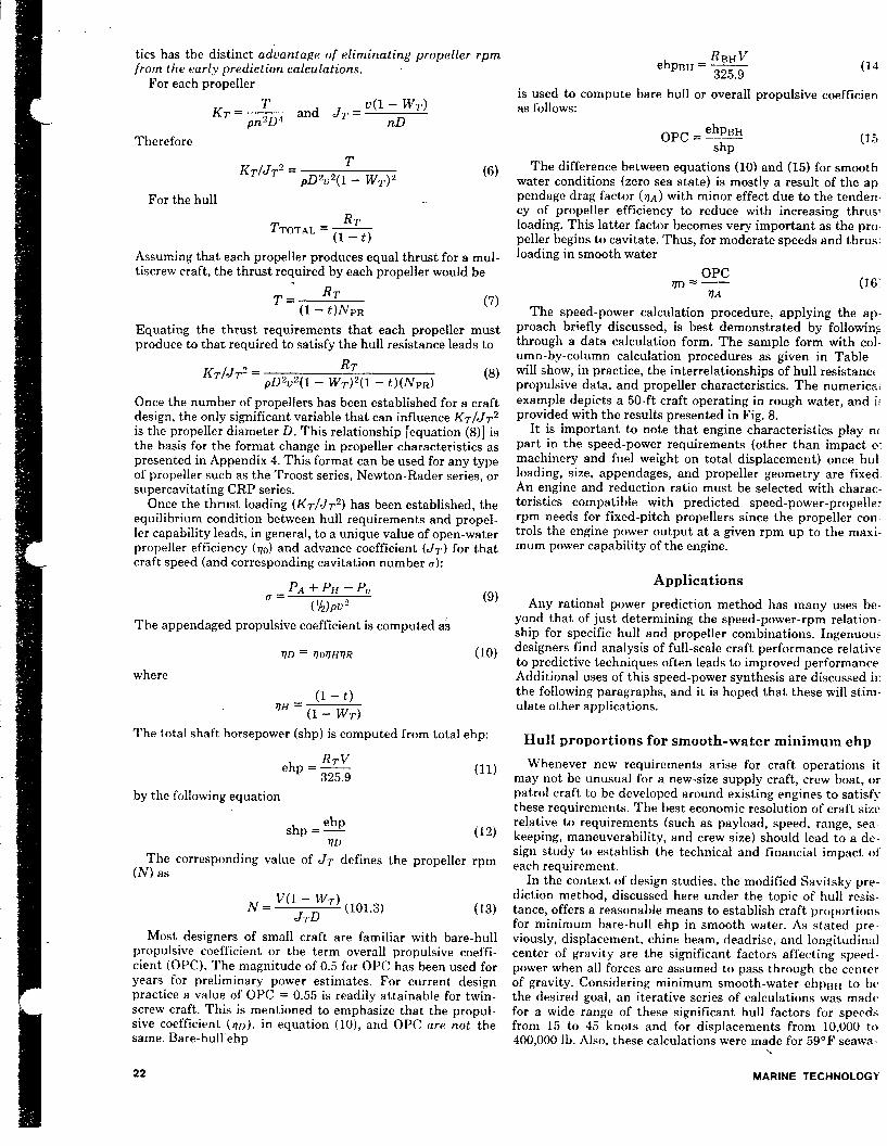
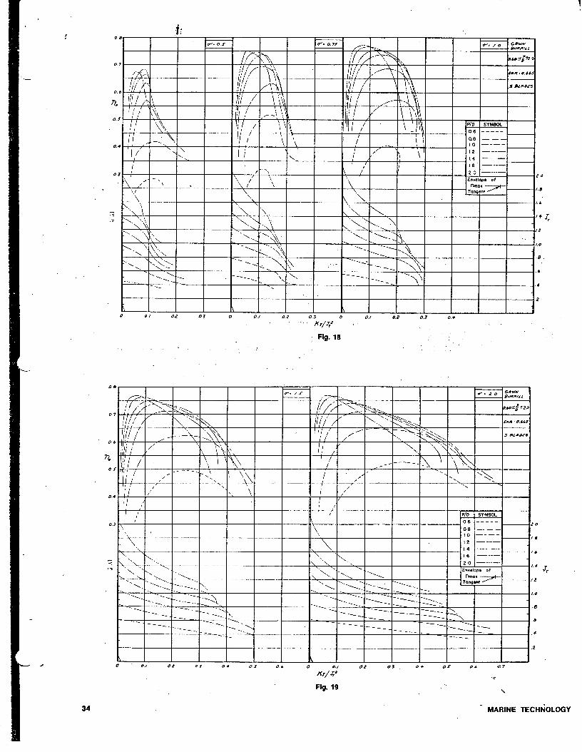
The Gawn-Burrill propeller characteristics are in the form of Kr, Ku, ~0, versus Jr for various pitch ratios, blade area ratios, and cavitation numbers (0). This familiar format, however, can’be replaced with another yhich reduces the effort required to optimize the propeller, select the reduction ratio, and make the speed-power-rpm predictions. This format is that of ~0 and JT versus KT/JT’ for various P/D, EAR, and CL The entire Gawn-Rurrill propeller series has been redone in this format and is presented in Appendix 4. The effort required to recompute and redraw these curves is compensated

JANUARY 1976

for by the long-term savings in preparing performance predictions and optimizing propulsion systems.

Power prediction method

The material presented up to this point have noted data sources and logic leading to assumptions necessary to establish the data base for making a power prediction for craft. Now is the time to put it all together.

It is important to keep one thought in mind when working with propellers. Propellers produce thrust. While engine power is converted to thrust horsepower by the propeller, selecting a propeller to absorb power at a particular rpm and speed does not necessarily yield the maximum speed poten- tial of a-craft. The following procedure describes the method to effect a speed-power prediction, beginning with speed resk- tance and then establishing the thrust requirements.

The development of KT/J T2 as the common variable between hull thrust requirements and the propeller characteris-

21

tics has the distinct advantage of eliminating propeller rpm from the early prediction calculations.

For each propeller

KT T

= - and JT = v(l- WT) *

pn2D4 nD

Therefore

KTIJT~ = T

pD2v2(1 - wT)2 (6)

For the hull _.

TTOTAL = RT

(1 - i) Assuming that each propeller produces equal thrust for a mul- tiscrew craft, the thrust required by each propeller would be

T; RT (1 - t)NPR

(7)

Equating the thrust requirements that each propeller must produce to that required to satisfy the hull resistance leads to

KT/JT~ = pD2v2(1 - wT)2(1 - t)(NpR)

(8)

Once the number of propellers has been established for a craft design, the only significant variable that can influence KT/JT~ is the propeller diameter D. This relationship [equation (8)] is the basis for the format change in propeller characteristics as presented in Appendix 4. This format can be used for any type of propeller such as the Troost series, Newton-Rader series, or supercavitating CRP series.

Once the thrust loading (Kr/Jr2) has been established, the equilibrium condition between hull requirements and propeller capability leads, in general, to a unique value of open-water propeller efficiency (~0) and advance coefficient (JT) for that craft speed (and corresponding cavitation number a):

Pa + Pjj - Pu u=

(%bv” (9)

The appendaged propulsive coefficient is computed as

?lD = rlOr7HrlR (10)

where

(1 - t) rlH = (1 - w,)

The total shaft horsepower (shp) is computed from total ehp:

ehp RTV =- 325.9 (11)

by the following equation

ehP shp = - 770

(12)

The corresponding value of JT defines the propeller rpm 00 as

N v(r - WT) = JrD

(101.3) (13)

Most designers of small craft are familiar with bare-hull propulsive coefficient or the term overall propulsive coefficient (OPC). The magnitude of 0.5 for OPC has been used for years for preliminary power estimates. For current design practice a value of OPC = 0.55 is readily attainable for twin- screw craft. This is mentioned to emphasize that the propulsive coefficient (qn), in equation (lo), and OPC are not the same. Bare-hull ehp

ebBH RBHV =- 325.9 (14

is used to compute bare hull or overall propulsive coefficien as follows:

ehpRH OPC=7 (1 5 ShP

The difference between equations (10) and (15) for smooth water conditions (zero sea state) is mostly a result of the ap pendage drag factor (77~) with minor effect due to the tenden- cy of propeller efficiency to reduce with increasing thrus- loading. This latter factor becomes very important as the propeller begins to cavitate. Thus, for moderate speeds and thrus: loading in smooth water

OPC rlD w- (16 1

rlA

The speed-power calculation procedure, applying the approach briefly discussed, is best demonstrated by following through a data calculation form. The sample form with column-by-column calculation procedures as given in Table will show, in practice, the interrelationships of hull resistance propulsive data, and propeller characteristics. The numericaL example depicts a 50-ft craft operating in rough water, and i> provided with the results presented in Fig. 8.

It is important to note that engine characteristics play n< part in the speed-power requirements (other than impact 01 machinery and fuel weight on total displacement) once hul loading, size, appendages, and propeller geometry are fixed. An engine and reduction ratio must be selected with characteristics compatible with predicted speed-power-propeller rpm needs for fixed-pitch propellers since the propeller con- trols the engine power output at a given rpm up to the masi- mum power capability of the engine.

Applications

Any rational power prediction method has many uses beyond that of just determining the speed-power-rpm relationship for specific hull and propeller combinations. Ingenuous designers find analysis of full-scale craft performance relative to predictive techniques often leads to improved performance. Additional uses of this speed-power synthesis are discussed in the following paragraphs, and it is hoped that these will stim- ulate other applications.

Hull proportions for smooth-water minimum ehp

Whenever new requirements arise for craft operations it may not be unusual for a new-size supply craft, crew boat, or patrol craft to be developed around existing engines to satisf? these requirements. The best economic resolution of craft size relative to requirements (such as payload, speed, range, seakeeping, maneuverability, and crew size) should lead to a design study to establish the technical and financial impact of each requirement.

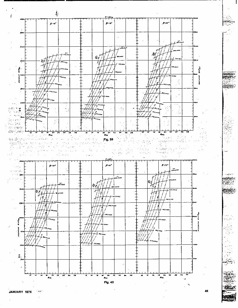
In the context of design studies, the modified Savitsky prediction method, discussed here under the topic of hull resistance, offers a reasonable means to establish craft proportions for minimum bare-hull ehp in smooth water. As stated previously, displacement, chine beam, deadrise, and longitudinal center of gravity are the significant factors affecting speed- power when all forces are assumed to pass through the center of gravity. Considering minimum smooth-water ehpBH to be the desired goal, an iterative series of calculations was made for a wide range of these significant hull factors for speeds from 15 to 45 knots and for displacements from 10,000 to 400,000 lb. Also, these calculations were made for 59’F seawa-


.

ter and zero correlation allowance. The iteration was effected by makin, u incremental increases in chine beam until minimum ehp~~,~ was obtained while LCG/Rp.x, deadrise, displacement, and speed were held constant. Thus, both LCG and Rp,y increased at a constant rate during the search for minimum ehpiJl+

This optimization process is illustrated graphically in Fig. 9 for one condition of displacement, deadrise, and speed. The results of these calculations are presented in Appendix 5 as contours of LCG/R p_y and displacement (W) relating minimum ehpl{H and maximum chine beam (BPx). Each figure of Appendix 5 is for a constant speed (assumed design speed) and gives results for deadrise angles of 10 deg, 16 deg, and 22 deg. I

These conditions for minimum ehpRH in smooth water permit interesting speculation if one does not introduce extrane- ous thoughts. (The authors are well aware that other factors, such as constructed weight, seakeeping, payload, cost, longitudinal and traverse stability, affect craft proportions. This application (Appendix 5), however, is limited to smooth-water speed-power.) hlost designers know, and these data show, that “real” hard-chine craft are too heavy relative to their size. Since the ratio of LCG forward of transom to length overall (LCGILOcl) is usually in the range of 0.37 to 0.40, it might take a zero payload condition for a craft to operate at a hydrodynamic condition for minimum power. (Example: At 30 knots, 8 = 16 deg, and a displacement of 100,000 lb, an overall craft length of 90 to 95 ft would result in ehpBH of 1000 on a craft with 16-ft chine beam.) Thus, a 90 to 95 ft craft could at- tain 30 knots with approximately 1820 shp (OPC = 0.55) at a displacement of 100,000 lb. But, could a craft of these proportions and power be constructed with adequate allowance for fuel and useful payload?

It is interesting to note that for speeds of 30 knots and above, designers can relegate chine beam (BP&~) to a position

. of minor consideration relative to powering requirements (see Appendix 5). Thus BP,~ can be selected for other important reasons such as seakeeping, internal volume,‘deck area, or transverse stability as discussed in reference [4].

Many tradeoff relationships can be extracted from Appen- dix 5. Figure 10 shows the effect of design speed on the selection of chine beam for minimum ehpBr_i in smooth water. Like- wise, other tradeoff relationships, such as deadrise effects on ehpi3H as shown in Fig. 10, may be extracted as user needs arise.

Selecting best propeller and reduction ratio

The “best propeller” for a craft is that which satisfies the craft thrust requirements within geometric, financial, and power limitations. If there were no design constraints, an “optimum propeller” could be designed for maximum efficiency. With this slight distinction of terminology, optimum propeller and best propeller are not considered to be equivalent and the term “best propeller” will be used here.

The geometric constraints to be considered may well pre- clude the selection of an operationally suitable propeller. Thus, it is important to establish the maximum propeller dimensions allowable for the shaft angle, tip clearance, and draft limitations. Most craft have shaft angles in the range of 10 to 16 deg measured relative to buttocks, and propeller tip clearance of 15 to 25 percent of diameter. Smallest shaft angles are generally employed on craft with highest design speeds, and tip clearances are controlled to a large extent by propeller-induced vibration, which is often traced to extensive cavitation.

The key to selecting a best propeller to satisfy the craft propulsion needs rests with equating required craft thrust with

JANUARY 1976

propeller thrust. Equation (8) defines the thrust-speed-propeller diameter relation as required for equilibrium conditions, and the speed-power calculation form should be followed. First, assume three or more values for propeller diameter, not exceeding geometric constraints, and assume three values of cavitation numbers corresponding to speeds above and below the design speed. Perform the calculations from Column 1 to Column 11 according to the procedure described in Table 1 for each combination of speed and diameter. Rec- ord in Column 20 the propeller diameter used in each line of the calculations.

Based on previous experience a designer will usually have an estimate of the expanded area ratio of propellers on similar craft. If so, the closest value of EAR available in the Gawn- Burrill series (Appendix 4) should be used with the propeller characteristics for the remaining calculations. (Some guides for approximate values of EAR are as follows: Three-bladed conventional stock propellers, use EAR = 0.51; three- bladed wide-blade stock propellers, use EAR = 0.665; four- bladed conventional stock propellers, use UR = 0.665).

For kach line, use the values of KrlJr2 and u from Columns 10 and 11 to enter the appropriate propeller characteristics curves in Appendix 4, and locate the maximum value of efficiency (~0) for -that thrust loading. Record the maximum ~0 and corresponding (JT) and (P/D) in Columns 12, 13, and 21 respectively. The calculation form is then completed Column 18. Compute pitch and record in Column 23.

These data are plotted as ShP, rpm, and pitch versus speed for curves of constant prop leller diameter. Construct a horizontal line at the installed power level that intersects the pre- dieted speed-power curves. Construct ver tical lines passing through each speed-power intersection point up to the speed- rpm and speed-pitch curves for the corresponding propeller diameter. These intersecting points are then plotted on a base of propeller diameter, that is, (i) speed versus diameter at design power; (ii) rpm versus diameter at predicted speed for design power; and (iii) pitch versus diameter at predicted speed for design power. This process is illustrated in Fig. 11 with intersection points identified in both graphs. The ratio of propeller rpm to engine rpm yields the desired reduction ratio. Slight adjustments in propeller pitch are usually required to match .stock gear ratios. A numerical example of this propeller selection procedure is presented in Table 2 and Fig. 11.

through

While this procedure establishes the best propeller diameter and pi tch for the assumed EAR, it does not establish that the blade area is adequate relative to cavitation effects other than from a perform ante point of view. Important factors affecting both the hul 1 structura Id .esign in the vici .nity of the propeller and the blade cavitation damage m ust be considered. Blade rate-induced hull pressures on the ord er of 4 to 5 psi can be generated by a badly cavitating propeller, and can fatigue (crack) hull plating after short periods of operation. Likewise, these blade cavities can be destructive to the propeller, eroding blade material to the point of requiring frequent propeller replacement.

These effects can be minimized by carefully selecting EAR such that 7~ (a thrust loading coefficiency related to pressure) does not exceed the 10 percent back cavitation relationship defined by Gawn-Burrill [18]. Thus, if

7c ,< 0.494(a()JR)0.88 (17)

(an ap proximation of the Ga .wn- Burril 1 10 perce lnt back cavitation criterion), one can be con fident tha t the propeller has adequate blade area. TC and a(j.7~ take into account the resultant of both rotational and axial velocities and are computed as follows:

(text continued on page 26)

23

Table 1 Propeller selection and speed-power calculation procedure

a--

-

r/ 7. i r ._

I 9pDs 1 7. I T

IJ r

r2 fO.0 2287 J2s 343 2755 a98 0.92 J.060 LO .3* .bfo 1.08 .% 85 ISJ 441 A3.0 3.71 70 .46 I2 r3 12.5 4785 273 7J7 577s r-23 /.NS .455 .eo .9? .5J 221 433 612 J2.i 4.15 I J83 AZ B

14 /so, 609J 368 913 7372 I. 4 7 /.Ola .382 .GZO * I.02 -54 339 , &2s bB8 /se 4.67 I ,280 .4 5 4 17.5 1

IY_ &758 439 /o/3 82/O /.77 J. O/O .332 - 1 ,040 r.ole .58 441 7&O 1 751 4 -- I/7.5 $7/t% 1 I 362

. IG 19.82~ N80 485 /o&a 8521 I.94 “t” 0.995 w 1.14 .91 518 849 779 /9.82 544 424 /7 2209 G8G9 S/7 1030 8416 2.24 6.975 .ti3 I.50 .700 1.21 .&PG 591 895 830 n.s9 rrs/ 482 18 28.04 tsG& 578 980 812s 2.75

I 0.970 .I39 /.oo .745 1.35 .?I 699 984 907

1 I 28.ab so3 St64

32 37 ~342 6.31 9S/ 7? 27 3. J? 0.980 .m 0.75 .735 1.42 .bv 787 II 46 100 5 32.37 A.45 629 .54 In to 13965 LP43i BJ/ 969 BZOb 3.s9 t 0.9751 1 .Ob? 0.50 .6?0 I.42 .&3 998 1 I584 fZZ& 39.65 3.u 782 49 po

CR~CULRT~~AJS FOR p@&D/CT/bh/ SkloWIv /A/ Ft’G UR E - 8 Pa /OP 1175

Data Craft Date Calculated bv Displacement LCG

Bpx P P

V

AC/l Sea state p,

Depth 4 of propeller

D (in.) D (ft) P (in.) p (ft) P/D EAR No. of blades No. of shafts


Description Craft identification Date of computation Person making computations Displacement of craft (lb) LCG of craft measured from

aftmost point of planing . bottom (ft)

Maximum chine beam excluding external spray rail (ft)

Deadrise at mid-chine length (deg )

Mass density of water (lb sec2/ft4)

Kinematic viscosity of water (ft? /set)

Correlation allowance Nominal sea state Vapor pressure of water

(lb/ft2) Depth to e of propeller hub

measured from water surface with craft at rest (ft)

Propeller diameter (in.) Propeller diameter (ft) Propeller pitch (in.) Propeller pitch (ft ) Propeller pitch ratio Propeller expanded area ratio Number of propeller blades Number of propeller shafts

l

Cd. I.

2. 3.

4.

5. 6. 7. 8. 9.

10. 11. 12. 13.

14.

15. 16. 17. 18. 19.

20. 21.

22. 23. 24. 25. 26.

NOTE: Lines 1 to 10 may be used for propeller selection or speed-power calculations.

Data Speed

RowsltolO Rows 11 to 15 Rows 16 to 20 Bare-hull resistance Appendage resistance

Source

Added resistance in waves (0 f-or calm water)

Total resistance Volumn Froude No. Thrust deduction factor Thrust wake factor Relative rotative efficiency Thrust loading Cavitation No. Propeller efficiency Advance coefficient based

on thrust

Assumed values Assumed values for V s 20 Computed for o of Cal. 11 Model tests or predictions Computed sum of shafts, struts,

rudders, etc. or estimated from Eqs. (4) and (5)

Model tests or Ref. [15]

Sum of Cols. 2, 3, and 4 Computed from Eq. (2) or Fig. 4 Model tests or Fig. 6 Model tests or Fig. 6 Model tests or Fig. 6 Computed from Eq. (8) Computed from Eq. (9) Obtained from propeller charac-

Appendaged propulsive coefficient

Total ehp Shaft horsepower Propeller rpm Speed Trim relative to mean

buttock Propeller diameter* or extra Optimum P/D* or extra

teristics for Cavitation No. and KT/JT~ at proper P/D and EAR (Appendix 4 of this report for Gawn-Burrill props.)

Computed from Eq. (10)

Computed from Eq. (11) Computed from Eq. (12) Computed from Eq. (13) Repeat of Cal. 1 Model tests or prediction

Assumed values From Appendix 4 for v0 opti-

mum EAR* or extra Propeller pitch* or extra Bare-hull ehp Overall propulsive coefficient Extra

. Assumed values Computed from Cols. 20 and 21 Computed from Eq. (14) Computed from Eq. (15)

. . * Data used for propeller selection.

Fig. 8 Predicted shp, rpm, and trim versus speed for calculated example

3ANUARY 1976 25

IO J5 LO 25 3e’ 35 40 4s SP&ED (& 1s)

v= 30 k p IG’

I I

15 /G 47 1s 19 20 21 Z?

. . BP4

Fig. 9 Graphical representation of process for establishing minimum ehpsH

c’

Fig. 10 Effect of design speed on S,, and minimum ehpsH variation with deadrise

The data for these criteria are presented in Fig. 12. The propeller selected in the example shown in Fig. 11 should have an EAR = 0.82 to satisfy the 10 percent cavitation criterion at maximum speed. Since this value of EAR is greater than that used for the propeller selection calculations, it should be repeated for EAR = 0.82 to be certain the best propeller has been obtained.

Should the value of EAR exceed 0.72 to 0.75, then it is un- likely that a stock propeller can be purchased. If this occurs, the designer has the choice of preparing a custom propeller design or obtaining relief from geometric constraints to permit use of a larger-diameter propeller to reduce 7~ to an accept- able level. l

Full-scale performance analysis

Builder’s acceptance trials are the true test of the craft design effort as interpreted by the designer. The detail with

_W’ -_ - _ 0-

26

which the builder reproduces the design detail is reflected in overall craft performance. In order to rationally interpret trial results it is necessary to document the size and location of aZI underwater appendages, measure the propeller pitch and diameter, note the leading edge detail of the propeller, measure craft displacement and LCG.

In order of experience with problems related to low trial speeds, the authors have found the No. 1 cause to be stock propellers with blunt or thick leading edges, or both, or nominal pitch no better than =tl in. The second most frequent of- fender is overweight construction relative to preliminary ac- cepted weight estimates. (Either better weight estimates or better weight control during construction are required to avoid this problem.) Jn third place is the incorrect allowance for drag during performance predictions. Also, craft that have been in service for some time are often inflicted with a heavy coat of marine growth which results in speed loss. Docu- menting and solving craft performance problems is in itself an interesting career not unrelated to that of a detective. (Propel- ler vibration and local blade erosion problems do not come within the context of this report.)

Data acquired from most limited trials will consist of visual inspection of underwater portions of craft, some estimate of displacement and LCG, and speed versus rpm up to dead rack

‘\

MARINE TECHNOLOGY

t’

x._ r 1.A ‘A

L

L

c I I ZS .

_.

’ 2000

- 1500

I

I

P k 01

-

Fig. 11 Plot of calculation example for propeller selection

JANUARY 1976

(and maybe fuel rate) measured in deep water. Obtaining power measurements during trials, however, is invaluable for propulsion system analysis, with thrust measurements being the most sought after but least often obtained data.

A common problem experienced during trials is failure of the engine to reach rated rpm. The obvious solution is to reduce the propeller pitch until the proper engine speed is at- tained and then accept the resultant speed. This is an example of selecting a propeller to absorb power rather than attempting to obtain best craft performance.

It is very possible for the propeller to be too big in terms of pitch or diameter or both. Trying to isolate the cause, however, could lead to a best resolution as to excessive hull resistance or reduced propulsion efficiency. Using the resistance prediction methods or experimental data sources available, the hull contribution can be established reasonably well. Trial speed, rpm, and propeller eometry can lead to a representative full-scale shp estimate as shown in the following table:

TRIAL DATA LL___ &X____ EAR_ W- LCG_

Trial data

Computed As- from trial sumed, data Fig. 6

1 - WQ JQ

Compute from JA alld (1. WQ)

KQ ShP I Prop. Com- charact- puted eristics

An alternative method to determine shp for diesel engines is to measure fuel rate and obtain shp from engine characteristics. By computing the estimated OPC the designer can make comparisons with that value used fdr preliminary speed-power estimates. A low value of OPC implies low propeller efficiency or high appendage resistance. Detailed calculations of appendage resistance can be made from the information summa- rized in Appendix 2 EO verify or eliminate the appendages from consideration as the source of the propeller overloading. Assuming JQ = JT, the foregoing calculations can be carried on to 7~ and ag.7~. If these computed valuesexceed ihe KT breakdown curve in Fig. 12, the full-scale propeller is operating at lower efficiency than technically attainable. Should low propeller efficiency be the cause of engine overloading, the best solution is changing to a refined propeller design rather than just reducing pitch to absorb rated engine power at proper rpm.

Power measurements during trials of newly designed craft would be of great interest to builders and operators. This would provide a rational basis for establishing technical achievement and refinement of stock designs. With these data, performance analysis (propulsion problem solving) is reduced to a technical exercise ~aher than a speculative art.

Concluding remarks

We are in a period where data obtained in the past or data spun off from other technology programs are being applied to craft design processes.

This effort was directed toward organizing and applying reference material that exists for the small-craft designer in the area of performance prediction. Others, however, have and will perceive different uses of these data. By exposing this effort for inspection, the true value will be established by the di- alogue that follows.

28

Acknowledgments

This work has been carried out as part of the Combatant Craft Improvement Program sponsored by the Naval Sea Sys- tems Command. The authors would like to express their thanks to the various members of the Navy community for supporting this project.

Without the contributions of other authors, this material could not have been compiled. We are indebted to each of the authors whose material was referenced and who influenced this approach. Miss E. N. Hubble and Mr. G. 0. Takahashi deserve special attention for their respective efforts of computation and drafting to produce the propeller curves in Appen- dix 4. Also, we wish to thank Mrs. Alice Waller for preparing the manuscript.

The preparation of this paper took a considerable amount of time from the normal family routine. We found the pa- tience, understanding, and support of our families to be an essential element to bring this effort to fruition.

References

1 Hadler, J. B., “The Prediction of Power Performance on Plan- ing Craft,” Trans. SNAME, Vol. 74, 1966.

2 Hadler, J. B. and Hubble, E. N., “Prediction of Power Perfor- mance of the Series 62 Planing Hull Forms,” Trans. SNAhlE, Vol. 79, 1971.

3 Du Cane, P., High-Speed SmaZZ Craft, John de Graff, Inc., Tuckahoe, New York. .

4 Savitsky, D., Roper, J., and Benen, L., “Hydrodynamic Devel- opment of a High-Speed Planing Hull for Rough Water,” 9th Sympo- sium on Naval Hydrodynamics, Aug. 1972.

5 Savitsky, D., “Hydrodynamic Design of Planing Hulls,” MA- RINE TECHNOLOGY, Vol. 1, NO. 1, Oct. 1964.

6 Clement, E. P. and Blount, D, L., “Resistance Tests of a Sys- tematic Series of Planing Hull Forms,” Trans. SNAME, Vol. 71,1963.

7 Hubble, E. N., “Resistance of Hard-Chine, Stepless Planing Craft with Systematic Variation of Hull Form, Longitudinal Center of Gravity, and Loading,” NSRDC Report 4307, April 1974.

8 Holling, H. D. and Hubble, E. N., “Model Resistance Data of Series 65 Hull Forms Applicable to Hydrofoils and Planing Craft,” NSRDC Report 4121, May 1974.

9 Hadler, J. B., Hubble, E. N., and Holling, H. D., “Resistance Characteristics of a Systematic Series of Planing Hull Forms-Series 65,” SNAME, Chesapeake Section, May 1974.

10 Kapryan, W. J. and Boyd, G. M., Jr., “Hydrodynamic Pressure Distributions Obtained During a Planing Investigation of Five Relat- ed Prismatic Surfaces,” NACA Technical Note 3477, Sept. 1956.

11 Hoerner, S. F., Fluid Dynamic Drag, published by the author, Midland Park, N. J., 1965.

12 Gregory, D. L. and Dobay, G. F., “The Performance of High- Speed Rudders in a Cavitating Environment,” SNAME Spring Meet- ing, April 1973.

13 Mathis, P. B. and Gregory, D. L., “Propeller Slipstream Perfor- mance of Four High-Speed Rudders Under Cavitating Conditions,*’ NSRDC Report 4361, May 1974.

‘14 Fridsma, G., “A Systematic Study Of The Rough-Water Per- formance of Planing Boats,” Davidson Laboratory Report R- 1275, Nov. 1969.

15 Fridsma, G., “A Systematic Study of the Rough-Water Perfor- mance of Planing Boats (Irregular Waves-Part II),” Davidson Labo- ratory Report R-1495, March 1971.

16 Blount, D. L., Stun@ G. R., Gregory, D. L., and Frome, M. l J., “Correlation of Full-Scale Trials and Model Tests for a Small Planing Boat,” Trans. RINA, 1968.

17 Blount, D. L., “Resistance and Propulsion Characteristics of a Round-Bottom Boat (Parent Form of TMB Series 63),” DTMB Ke- port 2000, March 1965.

18 Gawn, R. W_ L. and Burrill, L. C., “Effect of Cavitation On the Performance of a Series of 16-Inch Model Propellers,” Trans. INA, Vol. 99, 1957.

Discusser

Eugene R. Miller \

MARINE TECHNOLOGY

040

.oY

.a8

l 07

l O b

Fig. 72 General trend of Gawn-Burrill propeller series cavitation phenomena

Appendix 1

Savitsky equations

Solve-for 7:

CL0 = l-l 0.012 VT + 0.0055x5/2’

T (W * 2

V

Equations for resistance and ehp computations by Savitsky ‘Ompute for um’ method when all forces pass through CG [5] (Given: W, LCG, BPX, I% P, v, ACA, Vk

O.OlZt/j; + - 0.0065~(0.012~ T~-~)*.~ 1~ bl

x COST - 1 Computed from given data: Compute for Re:

(20) Re vnl m PX =- (26)

Computed froIllgiven data:

CLp = W

(?!~P~~BPx~

Solved for A: 4

cp = LCG

- = 0.75 - BPXX

.

r l 1

1 5.21(C,)2 ‘ XL

Solve for 0: ._

Cb = CL* - 0.0065 p CL,p$6

JANUARY 1976 29

)

(23)

(Schoenherr friction formulation)

Compute for RBH:

RBH = W tan7 + Pm “ABpx2(Cfi* + AC/q ) . -.

2( cos/J) (COST) (28)

Compute for ehpsH:

ehpF3H = Rwv .’ (29) 325.9

\

4

-

-

Appendix 2

Appendage resistance

Inclined cylinder, that is, shaft and strut barrel:

DSH = % Zdu2(1.1 sin3, + ?rC&

Skeg: _.

DK =

Strut palms:

where

CDp = 0.65

and

6 = 0.016Xp

Nonvented rudders and struts:

DRIS = P ;sv22cF

t t 4 1+2-+60 -

c 01 c

Interference drag:

DZP p2t2 [0.75 f) -o.ooo3/(~)2] Nonflush seawater strainers;

where

Do = - ’ &h 2cDo 2

CD* = 0.65

(30)

(31)

(32)

(33)

(34)

(35)

Experimental rudder drag coefficients in a propeller slipstream

Geometric aspect ratio = 1.5

KT/JT2 = 0.20 Propeller 0.55 D ahead of rudder stock

cDR t/c 0 = 4.0 0 = 2.0 CT = 1.5

-I 0 = 1.0

t L

I 1 I I I 1 NACA 0.15 0.0015 0.0015 0.0015 0.0008

0015

I Parabolic 0.11 0.0417 0.0427 0.0433 0.0425

(blunt base)

I I I I I 1 Flat plate / 0.04 1 0.0278 / 0.0325 / 0.0371 / 0.0433 1

I6-deg 1 0.11 e/ 0.0495 1 0.0495 1 0.0495 1 0.0487 1 wedge

DR = P -&CD, 2

Range 0.3-0.9 3-6 0.06. 3-7 lo-30 to 0.8 to 6 1 / 1 1 1 0.18 1 deg 1 deg 1

Added resistance in waves (Figs. 13 and 14). The chart in Fig. 13 is entered with a given trim and deadrise. (RAW/

‘\


Appendix 3

Added resistance in waves

This work was extracted in part directly from reference [l53 with permission of the Davidson Laboratory. The following is reproduced here so that the user of this prediction method might have one complete reference source containing material to account for all items to be considered. It is essential that reference [15] be consulted for complete understanding and application of this method of accounting for added resistance in waves.

Different notation was used for equivalent data descriptions between this report and reference [15]. These differences are:

Reference [ 143 (Fridsma)

SMALL-CRAFT power prediction

(Blount-Fox)

b BPX L LP RAW RA A W

. . Design Charts

The ultimate goal for this study is to enable designers and those interested in planing craft to use the information gath- ered herein in a practical and meaningful way. Working charts, with appropriate correction factors, were constructed so that the results could be immediately applicable to the prediction of full-scale performance of planing hulls. Some details of the effects of individual parameters can be gleaned from the charts and equations; but this is discussed in the next section in a more generalized way. In this section the reader will be shown how to use these charts, and what corrections are applicable, as well as a number of worked examples.

To enter the charts and determine a prediction for a given boat, seven quantities must be known; namely, displacement, overall length, average beam, average deadrise, speed, smooth- water running trim, and the significant wave height of the irregular sea. Since realistic boats do not normally have a constant beam or deadrise, it is suggested that these quantities be averaged over the aft 80 percent of the boat. It is understood that the designer has recourse to smooth-water prediction methods [5] which will enable an estimate to be made for the resistance, trim, and rise of the center of gravity as a function of forward speed.

The nondimensional parameters are calculated next, such as CA, L/b, VA/L, and H&b.

In using the charts, the designer should be careful not to make gross extrapolations. The charts are accurate within the ranges of test data. A reasonable amount of extrapolation has been built into the charts beyond the limits of the test data, and the results continue to be reliable. It is when parameters go far beyond the test ranges that one must be careful. The following guide should be helpful in establishing the limits of the use of the charts.

Para- meter G L/b G&lb 7 P H,/,/(5 VlJL

I

. .

-:.: 0.01 I .’ ! . -. ..; . i

I I

* . .

i:.:i : *’ *

. ’ ! I *.- . * .i

.

i.l i.* i I

. . .__ - 0

.:!i .I ’ . .: : .‘.-. : - “, **j; .I ] . ( ‘. . 8 .

1

.’ .‘I

Fig. 13 Maximum added resistance and speed for Cl = 0.60 and L/b = 5

6

Fig. 14 Generalized added resistance plot for CA = 0.60 and L/b = 5

JANUARY 1976

.

l

d ! f‘ t

* wb3hnax and (VIdL)*,,, are read off for the three sea states. An interpolation for the correct sea state can be made imme- ‘diately, or the added resistance can be obtained as a function of wave height. For a given V/dL or a series of speeds the ratio V/V*,,, is calculated, and RAW/RAW,,, is obtained from Fig. 14. The added resistance is found by multiplying the resistance ratio of Fig. 14 by the RA&wb3),,, obtained from Fig. 13. The result, however, is true for a CA = 0.6 and L/b = 5, and must be corrected by means of the following formulas: \_. < . -‘--. , - . fRA wIwb3)final = WA w/Wb3)charts

xE (CA, L/b, V/x& H1/3/b)

Added resistance corrections

I I V/i/L - E

2 1 + [gJ2- I]/[1 +‘.M(H,/,/b -- 0.06)] ._

4 1 + lOH,,,/b(Cn/L/b - 0.12)

I I 6 1 + 2HI,,/b[0.9(Cn - 0.6) - 0.7(Cn - 0.6)2]

Equa- tion

(1)

(2)

(3)

. . . .._ - _. For the particular values of CA and L/b, calculate E and ,. _.\ _^ ._ ;-_ * (V/dL),,, or‘ V/V,,, is*associated with the speed at which ’ plot as a function of V/A/L. Read off E at the V/A/L of inter-

(RA dtnax OCCUfS. _, * est to correct the added resistance value. *. . . \ ,- -’ ._ .* - . 7. .- . . . _ I*- ‘.,.,., . . _ . . . . ,_,-1. ,.-.-’ _I - _,, _.-.- .L’ . .L r* l .I-. . . . .: :. ._.‘_ ’ * ‘k . . . , . . ” .* ‘. z- . :- ‘. .- I -. ‘,a * #< . . . b I ..<. 8 . . - . , _ no . I . 9-T.-- \ . I - ~.-TT.‘- ‘Vs. .; .., _* 7. . . -.. : . .‘.i; 1 _ ,__~,~. .. -:; ~. :‘. . . ,. ̂

*La ’ ‘” -- bc . I _. _.. j !k’. . --- . _‘x-L_,.* _._ .~_ _ ‘..‘.w’ , \ c’.’ . -. -0 . I. _ Appendix 4 _

_ “X. ‘._ . * , < . * .’ - I r : : : :, _+. ‘. ~1 .,_..A$- W-=” r‘ .‘*. . ’ b : I . ‘. . ~ *.; ‘ .: 1, , s_ _ ___ < I- *- ‘- . . . ’ . . . I * .,-; ,. .‘I5 . . r .’ . J Gawi_Burrill propeller characteristics,

’ .,. s I w “ . ‘. . . ~ , .., a ’ Y “~+” ’ ‘. . “.

‘._ \ ‘.

. ‘. \; lL - ___ _- -. 4 .8

\ ‘. “\.* . . . ‘A___,\ <’ _____. -- 9

. -6

.--__ -9 ‘\ --. -- --_ ---. \ l .+

- \

Fig. 15

(Appendix 4 charts, Figs. 15-31, continue through page 40. Appendix 5 charts, Figs. 32-40, begin on page 41.)

. . . ‘\

. 32 MARINE TECHNOLOGY

. --- _. / \ - / 4 / \ I

, -. .

/

f

If P/D SYMBOL / 0.6 m--w_

. . 1

1.6 ----I ’ f.8

20 -me_- - 1.4

I- i T- -- I J-2

. 0 0. / 0.2 0.3 0.4 0.5 0.6 0.7

’ KT /2,’ :: _.; .

Fig. 16 . - ; . .- - , . . 9 . _

‘r- I I I I I 1 1

3 A

)O -_-_

4 120 \ 1.2 ---- \

‘\ 14 -a- J 1.6 -_-- .I.8

-‘\__ -m

--_ -__ I * LO

--w_ f .e -

--.N_ --- --m__

--__

--- ---se.- ---_ -__ , .6

- - __ ---.-

----B-v_ m-m_ -

---_ --_

--- ----.--_._ 1 4 ----- ----__-_-_--c-e--

II I we

I)

. 0

33

-I \\ 0.6 _----

/ I 1

/ \ ‘I -. \ I 10 -_-_

I I I/’

\I 1

\

\ \’ , I.2 ----

I 1.4 --- I / I

// I . 1.6 - e-w- I

_ .Fig.18 ,’ .

__-- m __-

t-

II \ -x. 1.6 ----

\ ‘\ 20 -e--s \

Envclooo of

\ .

MARINE TECHNOLOGY

0 X7,$ Fig. 19

34

0.6 _----

AI ---

I

“.” ~-

1.0 ----

1.2 ----

1.4 ---

1.6 ---- 20 -.__s

Envelooo of

Kt/4a . _ .

Fig. 20 \. .

. . -

04

i ,* ‘-“.\, I1 I I f-

/ , \ I If

0.3 20

2.0

1.0

1.+

4 r2

I.0

-6

-4

2

Y\\- I I \ -

\ \ ‘. I

-. Fig. 21 , c \

JANUARY 1976 ’ ‘r

-- -‘r,

0.8 ---I 1.0 ----

1.2 ---- ,

1.4 ---

L Fig. 22 ._ . i

. . /

- .

I .

ac

36

Fig. 23 \ .

MARINE TECHNOLOGY

* I ( 0.6 m---m

2.0 I 0.8 - -- IA - p-w

. .-*. - .@ _ .A

. -3

I _

. . L

.

. .

; *

- .

- *

. t

- - , - .

-

:

. . .

‘i -.

. - .

.

_

-.: _*. _

. -

I

; _ . - , .

: . . ’ . ..’ _ _ .-,-,..

-. -. . _ ‘.a

“l : ‘_ ._‘4,. I *

. . . .

:

L’,

.8

II /

-2 .

\ 11 ** AA

Fig. 24 . .. . : .

8 . . . _.

” __ - ..-

_ . . . . _ .

, _ _- . .

,p/o srhmol_

0.6 w--v- I

i’l I I I I I I I I I I- - --- I. u

0.3 1.2

1.4

1.6

-9

Fig. 25 . . . . ‘\

JANUARY 1976 -.=t~ . \ w

2.0

J. 8

I.6

f-4

z2 J,

f.0

8

6

f

2

L I

1.6 ----

2.0 -e-w-

Fnwel- nf I

I I I I I I I I I I I _ 0 I I 0.1 02 I

0.3 a4 0.5 0.6 //;a 0.8 y?9 , l.0 L/

- . : . Fig. 26

0.t

0.7

. 0.6

' ?I

0.5

0.4

0.3

ti; P/D SYMBOL I 0.6 w - _ - m

I 0.6 ---

a..” ,

Envolopo of


. 1; / i \ I /

\\

I

\ /

\ \ \

I p/o I

___-._ 1 0.6 0.6 - -- 1.0 ---- . ,

I I

, . . .._ . _ * Fig.20 : ._._ ‘..I .,_ ‘_ . .L”-., _.- . . .

. . . :. . , .

‘08

0.7

06

rt

03

0.4

0.3

,

. . -

H c . ‘-4 ‘1

I ’ I I

- I i

p/o SY Ml3CX 0.6 _-___ 0.6 --- I.0 ---- ?. 0 1.2 ---- 1.4 --- a/.8 1.6 ---- 20 ____m

1 of nm0x -

-- Tongon? 1x4 1 1

I

06 0.7 08 ew

Fig. 29

39 JANUARY 1976 . -4

,

1.q --- I 1.6 ----,

- ,A8

2.0 B-_-m

Enwiopa of ’ I.6

------*T~f~~ f.4

. . I

O.dC

. 0.7 -

0.6 n

z?B -

0.5 -

04 -

0.3 -

Z

t; ”

L

L

L

0

-4

0.2 0.3

.

Fig. 30 t

, -

I I I I ,

I I 1 I I I I I 10.6 I----- 1

- 0.0---

‘I 1.2 1.0 ---- ---- -.-

I I I I I I I I I I I 1 1::; -__- k 2.0 1 --me- I

Envdopo of nmar P

I

40

KVJF= -e

Fig. 31 \

Conditions for minimum bare-hull ehp in smooth water computed from simplified Savitsky method as modified by equation (1)

. . .c .

. . .

. Calculations for zero correlation allowance, 59°F I 1 I seawater

. : _I _ _. . . ^ _. . . .a. . - ‘a-

._... . : m-

.’

_ ,‘&I- I .

. . . . . . . .

~ .

. _

- Fig. 32 _ . *

(Appendix 5 charts, Figs. 3240, continue through page 45.)

JANUARY 1976 -‘a 41

* ._ . . . \

. . . _ _ . _ ’

V*tOR

-t- I. I Ii\.’ Ii

42 MARINE lECHNOLO@

. . ’

Fig.& . _ - *. - _. .- ..:, : _ ‘*

.

_ .

. _’ *

:

’

. Fig. 36

\ \ .

3ANUARY 1976 :-:

-/ T- +

44 MARINE TECHNOLOGY ;

- _ E ‘3

-.._ _ . . . _- . .- \- . _ +.. * . 1 .‘. ..1 . . . I , .:a .- C... - ++*T. --, _-:

- ; . * , ; - * “ _ I-;‘ . __, :: . _- _ - -I . I X . L

_. ,Flg= 39 _ - ’ -‘--- ” ‘.- :- -: ; , - + . .

. __ . cc 3

.

- . : . .-” _ \ - . :’ (‘. . . . ‘...

. ‘_ _ - . ..* -._ -_‘ _., _I 1,. 1 ,,.; ..l ;;I;;.:: ;: 1 :.; ;.. --: I _

._- ,

- ‘.._ _. ., I .,h. -.. ; . : . .I -,

!. ._ . i’ . . - ,. ._ - 1 -._ -

, . 1 . . . . \

. * ->. . . . . .’ . . . ._

..* . . ‘..?,. .‘; . . . . . a .

. A . : . . I .- :-. ._. ‘. -. ;.; -. ., . L

. . .

. . . . . :-,.!,. ---. * . - . _. .

. ‘*... : : - .^.. ..!’ .I .-. . - . . . .II_--.* _

. _ -: <

. . . :.. .~ . .’

. . . - - ; . ‘.__ .’ i*.-‘. . ,- _ --

_: , ^ - . . . it _ :., _ : . ,-

JANUARY 1976 +;.”

: . _

. ,

small craft power prediction

Documents