smallholder oil palm: space for diversification?
TRANSCRIPT

Smallholder oil palm: space for
diversification? WaNuLCAS model-based exploration of the environmental and economic impact of
intercropping scenarios for Indonesian smallholders
MSc Thesis Plant Production Systems
Dienke Stomph January 2017
WaNuLCAS 4.3

2
Smallholder oil palm: space for
diversification?
MSc Thesis Plant Production Systems
Disclaimer: this thesis report is part of an education program and hence might still contain (minor) inaccuracies
and errors.
Correct citation: Stomph, D., 2017, Smallholder oil palm: space for diversification?, MSc Thesis Wageningen
University, 78 p.
Contact [email protected] for access to data, models and scripts used for the analysis
Name Student: Dienke Stomph
Registration Number: 930507808100
Study: MSc Organic Agriculture – Specialization Agroecology
Chair group: Plant Production Systems (PPS)
Code Number: PPS-80436
Date January, 2017
Supervisors: Meine van Noordwijk
Ni’matul Khasanah Tom Schut
Examiner: Maja Slingerland

3
ACKNOWLEDGEMENT
Firstly, I would like to express my sincere gratitude to supervisors Meine van Noordwijk and Ni’matul
Khasanah for their continuous support, assisting me, challenging me and allowing for independence.
I would also like to thank Tom Schut for his helpful remarks, which were of considerable support in
improving the structure of this final report. Furthermore, the fruitful discussions with people in my
close surroundings at Wageningen University and the World Agroforestry Centre scientists are
gratefully acknowledged.
FOREWORD
This MSc. thesis report describes the model development and simulation of plot-level diversification
scenarios for oil palm cultivation. The study zooms in to the Indonesian oil palm context, with as a
focal point smallholders on Sumatra. The report first lists the research aim and objective. After which
the contextual components of importance to this study are made explicit. The WaNuLCAS model (van
Noordwijk & Lusiana, 1999) is used as a tool to explore these scenarios, with the required inputs and
generated output. Then follows a section on the diversification scenarios and the indicators of interest
to measure and compare the scenario outcomes. As a last section in the methods, the calibrations and
modifications are described that were needed to equip the model to be suitable as an explorative tool.
Results of the scenario simulations are summarized and discussed in a broader context of recent
developments as well as the impact of this study on future developments.

4
ABSTRACT
This research aimed at challenging the assumption that oil palm is best suited to monoculture
cultivation for smallholders in Indonesia, through a model-based exploration of the short- and long-
term feasibility of a range of plot-level diversifications. The global palm oil production has increased
over fourfold in the last two decades, by converting forests and agroforests into monocultures, under
the assumption that monoculture oil palm cultivation is most productive. This deforestation caused
biodiversity losses and environmental degradation and raised social, political and economic concerns.
This study hypothesized that intercropping could serve as an integrative answer to several of these
concerns. As intercropping can deliver agronomic, economic and environmental system
improvements.
Intercropping was explored through simulation of five scenarios in the Water, Nutrient and
Light Capture model for Agroforestry Systems (WaNuLCAS) model. The 5 crops included were: cacao,
rubber, cassava, groundnut and mucuna as a cover crop. The scenarios were simulated for a 25-year
period, for four typical Indonesian oil palm weather and soil conditions. The prices of the farm inputs
(e.g. seedlings, labour, fertilizers) and produce were based on those recorded for the Indonesian
context. The intercropping scenarios were compared to the monoculture oil palm simulation based on
4 productivity and 6 environmental performance indicators. The model output was generated at plot-
level and therewith ignores interactions intercropping could have at farm- or landscape level.
The results showed that considerable economic and environmental system improvements can be
achieved through intercropping. With the exception of returns to labour, all indicators showed that
performance improvement was obtained. Compared to the monoculture, larger productivity per unit
of land, and environmental performance improvements were predicted for all intercropping scenarios.
Intercropping with cacao showed to obtain the largest net return to land, a 25% increase compared to
the monoculture, and can serve as a risk coping strategy. Including annuals in the first years of oil
palm cultivation resulted in the quickest investment recovery. Intercropping rubber performed poorly
for the economic indicators, but achieved the largest environmental system improvement. It is
therefore argued that diversification has a large potential to improve overall system performance at
both plot- and landscape-level. To utilize this potential more insight in smallholders’ interest in
diversification and suitable incentives to support diversification adoption by smallholder is required.

5
Table of Contents ACKNOWLEDGEMENT ..................................................................................................................................................... 3
FOREWORD ..................................................................................................................................................................... 3
ABSTRACT ....................................................................................................................................................................... 4
INTRODUCTION ............................................................................................................................................................... 7
AIM & RELEVANCE .......................................................................................................................................................... 8
BACKGROUND ................................................................................................................................................................. 9
Sumatran oil palm context .............................................................................................................................................. 9
The Sumatran environment .............................................................................................................................................................................. 9
A landscape in transition .................................................................................................................................................................................... 9
The Sumatran smallholder .............................................................................................................................................................................. 10
Mis(sing)-information ........................................................................................................................................................................................ 11
Certification trend within smallholder context .................................................................................................................................. 11
Smallholders and diversification ................................................................................................................................................................. 12
Oil palm cultivation ....................................................................................................................................................... 13
MATERIALS & METHODS............................................................................................................................................... 14
Data input & model description ................................................................................................................................... 15
Diversification scenarios ............................................................................................................................................... 16
Annual intercrops ................................................................................................................................................................................................. 16
Perennial intercrops............................................................................................................................................................................................ 17
Decision criteria ............................................................................................................................................................ 18
Productivity indicators ...................................................................................................................................................................................... 18
Environmental indicators ................................................................................................................................................................................ 20
Spatial levels and stakeholders .................................................................................................................................................................... 21
Model preparatory steps .............................................................................................................................................. 21
Parameterization, calibration and validation requirements ..................................................................................................... 22
(1) Vegetative & generative oil palm calibration ......................................................................................................................... 22
(2) Planting density calibration .............................................................................................................................................................. 22
(3) Fertilizer response calibration ........................................................................................................................................................ 23
(4) Profitability module ............................................................................................................................................................................... 23
(5) Palm’s responsiveness to drought ................................................................................................................................................. 24
(6) Palm growth reserves ............................................................................................................................................................................ 24
(7) Age-dependent yield dynamics ........................................................................................................................................................ 25
Phyllochron dynamics .......................................................................................................................................................................................... 25
Management related yield losses .................................................................................................................................................................. 25
(8) Root density and distribution ........................................................................................................................................................... 25
(9) Soil initialization ....................................................................................................................................................................................... 26
(10) Light module .......................................................................................................................................................................................... 26
RESULTS ........................................................................................................................................................................ 27

6
Performance levels for diversification scenarios (I) .................................................................................................................. 27
Performance levels for diversification scenarios (II) ................................................................................................................. 29
Sensitivity analysis ................................................................................................................................. Error! Bookmark not defined.
Performance levels for soil types and drought length .................................................................................................................... 30
Upscaling from plot to farm ............................................................................................................................................................................ 31
DISCUSSION & RECOMMENDATIONS ........................................................................................................................... 32
CONCLUSION ................................................................................................................................................................ 34
References .................................................................................................................................................................... 35
APPENDIX 1– Sumatran Agro Climatic map & peatland distribution ........................................................................... 44
APPENDIX 2 - Common management practices in oil palm cultivation ........................................................................ 46
Field preparation ................................................................................................................................................................................................... 46
Weed control ............................................................................................................................................................................................................ 46
Fertilizer management ....................................................................................................................................................................................... 46
Pruning ........................................................................................................................................................................................................................ 47
Harvesting .................................................................................................................................................................................................................. 47
Re-planting ................................................................................................................................................................................................................ 48
Leguminous creeping cover ............................................................................................................................................................................ 48
Initial-phase intercropping ............................................................................................................................................................................. 49
Permanent intercropping ................................................................................................................................................................................. 49
APPENDIX 3 – a. Systematic diagram of the core module and the additional modules in WaNuLCAS. ....................... 50
APPENDIX 4 – Calibration: input data, graphs and statistical output .......................................................................... 51
APPENDIX 5 – Fertilizer input for oil palm .................................................................................................................... 54
APPENDIX 6 – Model soil and weather input................................................................................................................ 55
APPENDIX 7 – Density and Spacing: Cacao & Rubber ................................................................................................... 72
APPENDIX 8 – P-Fertilizer yield response ..................................................................................................................... 73
APPENDIX 9 - Graph of phyllochron time dynamics .................................................................................................... 74
APPENDIX 10 – Two examples of performance variability over drought and soil ....................................................... 75
APPENDIX 11 – Profitability module input ................................................................................................................... 76
APPENDIX 12- Spatial levels of importance and linked stakeholders .......................................................................... 77
APPENDIX 13- Annual cumulative yield per cropping scenario over the 25-year simulation ...................................... 78

7
INTRODUCTION
The recent global boom in vegetable oil demand drives expansion of oil crop cultivation (Trostle,
2008). Oil palm (Elaeis guineensis Jacq.) is one of the main crops to satisfy the growing demand, for it
has the highest vegetable oil yield per unit area and labour of all oil crops (Corley & Tinker, 2015; Sheil
et al., 2009). Indonesia has responded to this increased demand, turning 10 million ha into oil palm
plantations (Direktorat Jenderal Perkebunan, 2015). Within a decade the country became world's
largest palm oil producer, accounting for more than 50% of the global market share (FaoStat, 2016).
The crops’ high profitability can support economic prosperity of rural areas, giving formerly
subsistence farmers the opportunity to obtain a substantial income (Belcher et al., 2004). However,
this rapid expansion, has not been without controversy, since the oil palm plantations replaced more
diverse agroforestry systems and 56% of the expansion was planted after clearance of native forests
(Casson, 2000; Basiron, 2007; Koh & Wilcove, 2008). More issues add to the controversy around palm
oil production. A shift in farm practices from a diverse system, to a single crop system increases the
vulnerability of rural communities, especially since global prices of palm oil have shown to be volatile
(Vermeulen & Goad, 2006). Additionally, the currently promoted oil palm farming practices do not
allow for intercropping of food crops, which former land uses did (Joshi et al., 2000). Thus, the
production of palm oil may come at the cost of farm and regional food security (Sheil et al., 2009).
Additionally, oil palm plantations pose environmental threats, such as biodiversity losses and
environmental issues arising from the increased uses of pesticides and fertilizers. The land clearing
practices lead to soil quality degradation and related erosion and sedimentation damage (Sheil et al.,
2009).
Furthermore, the extent to which smallholders and local communities profit from conversion
to oil palm is debated, and practices are disconnected from the local farming context (Casson, 2000;
Potter, 2016). Growth of the oil palm industry accelerated with the involvement of large
agribusinesses, which through governmental regulation and their established market positions,
limited smallholder’s independence and negotiation autonomy (Bissonnette, 2016). This large
dependence is also due to the large-scale dominated character of Indonesia’s palm oil processing
industry, imposing smallholders to sell their fresh fruit bunches (FFB) to the single reachable mill
(Potter, 2016; Vermeulen & Goad, 2006).
The current palm oil production system thus shows opportunities and pitfalls. In order to benefit from
the opportunities oil palm as a crop has to offer, perceptive analyses have to be made on the trade-offs
linked to the production. In the advocated production system, it is assumed that oil palm grows best in
monoculture. However, it is this monoculture production system that causes the oil palm related
issues listed above. Intercropping was coined as a strategy to alleviate similar dilemmas in other
regions and showed able to achieve productivity increases and/or address environmental damages
(i.a. Godoy & Bennett, 1991; Iijima et al. 2003; Yildirim & Guvenc, 2005). In oil palm main reasons
underlying the assumption that oil palm performs best as a monoculture, such as easy mechanization,
low labour demands, need for large yield to satisfy the processing capacity; are relevant to large
agribusinesses, but to a lesser extent apply to the context of smallholders (Corley & Tinker, 2003;
Potter, 2016).
Oil palm expansion may have originated from large scale plantations, but in the last two
decades an increasing proportion of oil palm is managed by smallholders (Table 1). Smallholders tend
to diversify their oil palm systems, however, an agronomic exploration of a range of diversified oil
palm systems is missing, despite the current wave of oil palm research from a socio-economic and
policy perspective (Drescher et al., 2016; Gatto et al., 2015a,b; Klasen et al., 2016; Li, 2015; Cramb &

8
McCarthy, 2016). Therefore, gaining insight into which species are favourable to use as an intercrop,
and establishing guidelines to support diversification decisions, can play a crucial role to safeguard
economic and environmental prosperity, both at farm and regional level. With disappearance of
traditional practices, the knowledge of managing these complex systems rapidly declines, thus support
is needed (Deb et al., 2009).
Table 1.
Oil palm area (ha) by type of ownership in Indonesia, 1980–2010. Source: Direktorat Jenderal Perkebunan (2015).
Year Smallholders % Government estate % Private estate % Total
1980 6,000 2 200,000 69 84,000 29 290,000
1990 291,338 26 372,246 33 463,093 41 1,126,667
2000 1,166,758 28 588,125 14 2,403,194 58 4,158,077
2010 3,387,257 40 631,520 8 4,366,617 52 8,385,394
Modelling provides a suitable tool to explore such agronomic options, as a model is able to
synthesize and integrate experimental and conceptual understanding of a system (Matthews et al.,
2002). A model provides the opportunity to explore a wide range of scenarios, against low cost, within
a limited timeframe (Mulia & Khasanah, 2012). Several models can be used for oil palm as
monoculture crop (Hoffmann et al., 2014; Khamis et al., 2005), but do not allow intercropping. Models
suited to explore intercropping include: CropSys (Stockle et al., 1994), STICS (Brisson et al., 1998),
WaNuLCAS (van Noordwijk & Lusiana 1999) and the GroIMP modelling platform (appendixrueyer &
Infomiatik, 2004).
WaNuLCAS, a model describing Water, Nutrient and Light Capture in Agroforestry Systems, was selected for this study. As it had the potential to combine oil palm with a wide range of annual and
perennial intercrops in a realistic and most plausible way. The model required a number of
modifications to strengthen the foundation for scenario exploration.
AIM & RELEVANCE
To this end the research aimed at challenging the assumption that oil palm is by definition a
monoculture crop, by exploring the feasibility of intercropping options in oil-palm plantations. The
specific objectives were to adapt WaNuLCAS to enable quantification of short- and long term effects of
oil-palm intercropping and to compare five scenarios with respect to agronomic, environmental and
socio-economic aspects. It is hypothesized that the productivity of oil palm cultivation can be
improved through plot-level diversification, while maintaining or enhancing environmental
performance.
The scenarios consisted of five realistic intercrop options: cacao, rubber, groundnut, cassava and
mucuna (legume cover crop). These species represent a diverse range, in terms of agronomical
performance and demand (e.g. profitability and light-, nutrient-, and labour requirements), while
being available to the Indonesian smallholder. The model simulates plot-level performances of
diversification. But in Indonesia smallholders manage an area of 3.4 million ha of oil palm. Their
practices are thus also of relevance to larger spatial analysis scales.
Sumatra serves as the focal area for this study, as it is illustrative of general trends observed in
Indonesia, but in its most widespread form (McCarthy & Cramb, 2009). The model simulations
accounted for a range of four modelled environments, to represent part of the existing diversity in
Indonesia’s oil palm planting environments.

9
BACKGROUND
Sumatran oil palm context
The present oil palm production system is complex and is therefore best seen in its economic,
environmental and socio-political context, as well as with consideration of precedent land-uses.
Sumatra is taken as focal area for this analysis, because Sumatra is the main oil palm producing island
of Indonesia, having 66% of the total oil palm area, and 81% of the area under smallholder production
(Direktorat Jenderal Perkebunan, 2015; Potter, 2016).
The Sumatran environment
Sumatra is the most western island of the Malay Archipelago. It stretches from the northwest to southeast, with a latitude ranging from 5°51’ N to 5°59’ S, thus its midline is crossed by the equator. The entire island is classified as Af (equatorial, fully humid) according to the Köppen Climate Classification System (Kottek et al., 2006). The majority of Sumatra is classified as ‘wet’ (>200mm/month) for more than 7 months per year, with less than two consecutive dry months (<100 mm/month). The most pronounced wet area is along the Island’s west coast, here precipitation exceeds 400mm for at least two consecutive months. The very northern tip of the island, as well as the South-eastern part are distinguished by more pronounced dry seasons of 2-3 months, and are characterized as wet for less than 6 consecutive months (Oldeman et al., 1978; Appendix 1).
As the sixth largest Island on earth Sumatra has a large diversity in soil types. A main distinction can be made by the division in mineral and peat soils. The peat soils are estimated to cover 25% of the island (Miettinen & Liew, 2010) and are mainly located alongside the east coast (Appendix 1). Currently the peat soils are subject to a large range of studies because of the large carbon stocks present, the risk of environmental damage by peat fires, and the complications for agricultural management. This study includes scenarios for mineral soils only because reports of oil palm performance on peat soils are scarce.
The island’s forests are characterized by high floral and faunal biodiversity, containing over 10,000 plants species, 201 mammal species, and 580 avifauna species (Kementerian Kehutanan, 2003; Whitten et al., 2000 in Margono et al., 2012). However, this diversity is in decline (Wilcove & Koh
2010).
A landscape in transition
From early 20th century, at the time of the first transition, decrease of Sumatrans natural forest cover
began (Therville et al., 2011). This land cover change started by introduction of rubber seedlings by
farmers into their swidden systems. Overtime systems evolved into ‘jungle rubber’: a productive
system in terms of ecological functions, soil protection and water regulation, however at current
monetary desires these systems decreasingly meet farmer’s expectations. Stimulated by governmental
efforts, some of these rubber agroforests have gradually been transformed to “improved” monoculture
plantations (Joshi et al.., 2003). Since 1990 a new actor has gained ground, large agribusinesses,
supported by the local and national authorities, have introduced various schemes to gain access to
farmland. The majority of the land owned by these agribusinesses did not originate from land with
prior cultivation, but from secondary or primary forest. This caused 40% of Sumatran’s tropical
forests to be cleared within two decades (Figure 1), of which most is replaced by large-scale
monocultures of rubber, oil palm and Acacia mangium Willd. (Margono et al., 2012; Therville et al.,
2011).

10
The Sumatran smallholder
The Directorate Jenderal Perkebunan (2015), estimates that 2.2 million smallholder households are
managing 4.6 million hectares of oil palm (Table 1). This illustrates the small average size, especially
when compared to private estates, with sizes of 5,000 up to 50,000 ha. The group listed as smallholder
is highly diverse in their level of dependence.
The first group of smallholders were those stimulated by Governmental and World Bank funded
schemes (1978-1999), to become part of Nucleus Estates and Smallholders (NES). Within this group,
various degrees of independence and working conditions exist, depending on the associated estate,
and individual agreements between farmers and estates (Cramb & McCarthy, 2016). In 1995 these
schemes were replaced by “KKPA” schemes (Primary Cooperative Credit for Members). This scheme is
funded through private companies and therewith differs from the NES schemes. In both programs,
generally, the smallholders are responsible for the quality of the management and resulting palm oil
yield. However, their management practices are restricted to the procedures as defined by the estate.
Another group classified as smallholder is those in a ‘joint-venture scheme’ (JV). In such a JV, a
company develops and manages a plantation on land owned by a farmer, in return the farmer receives
an area based monthly rent (Cramb & McCarthy, 2016). This scheme is independent of governmental
Figure 1: Four maps showing the declining forest cover of Sumatra from 1990-2010 (Margono et al., 2012).

11
funding, however it is much assisted by the government through continued law-revisions, guarantying
availability of land and length of tenure. For instance, in 2007, the Indonesian government
reformulated their Plantation Law on investment (No. 25/2007) to change the initial plantation lease
time to 60 years with possibility of further extension (Potter, 2016).
A third group of smallholders is classified as independent, meaning self-managed, self-funded,
thus independent in terms of production. In terms of income, however, they often still dependent upon
the willingness-to-buy and price-setting of a nearby plantation or mill (Cramb & McCarthy, 2016,
Figure 2). About half of the Indonesian smallholders is independent
(Potter, 2016). Recently, in major oil palm producing provinces as
Riau and Jambi, these farmers, sometimes assisted by local NGO’s,
started to organize themselves into groups. This, in order to improve
their negotiation position and access to inputs, knowledge and
processing mills. The independent smallholders are mostly former
rubber plantation and jungle rubber farmers. Once transport and
processing infrastructures were in place, and rubber prices showed
unreliable, smallholders were attracted to plant oil palm. Most of
these smallholders are limited by investment capital and thus adopt a
strategy of stepwise intensification to gradually intensify their
production (Cramb & McCarthy, 2016; Rival & Levang, 2014).
Mis(sing)-information
Currently smallholders, especially those independent of larger estates, are less productive than private
estates. A main driver is the lack of access to high-quality inputs, as with appropriate levels of access to
inputs and infrastructure, farmers were able to reach comparable, and even higher yields than private
estates (Cramb & McCarthy, 2016; Cramb & Sujang, 2013; Hartemink, 2005). Similarly, Molenaar et al.
(2013) found that only 50 percent of the independent smallholders use hybrid planting material,
which strongly decreases their yield potential. Additionally, the study mentions, that farmers located
in remote areas face a main limitation of getting the palm fruit to the mill on time (within 48h after
harvest, Corley & Tinker, 2003). The lower productivity is thus mainly resulting from differences in
access, between private estates and smallholders. These access issues persist, as the current policy
orientation continues to support expansion of large-scale agribusiness at the expense of smallholder
systems, despite the promised political commitment to support smallholders and implementation of
associated institutional reforms (Bissonnette, 2016).
Certification trend within smallholder context
Recently, research institutes and NGOs have become increasingly aware of socio-environmental
damage resulting from the rapidly expanding oil palm sector. Through scientific and media reporting
oil palm criticism continued to spread, which urged investigation of more sustainable palm oil
production practices (Comte et al., 2012; Rist et al., 2010). Oil palm plantations often replaced
landscapes which provided important ecosystem services. Plantations eliminated ecosystems
characterized by their large carbon stocks and degraded biodiversity. Simultaneously, increasing the
risk of flooding and degrading variety of rural food and income resources. Furthermore, the techniques
Figure 2: For processing of their fresh fruit bunches smallholders depend on the presence and willingness of private mills or estate mills to buy their harvest. Which makes them dependent on haulers, as mills do not permit them to transport their own fruit (Potter, 2016). Picture by D. Stomph (2016).
12
used for land conversion have led to emission of large amounts of greenhouse gasses (Ivancic & Koh,
2016; Winarni & Sutrisno, 2014).
In response to these trends, the international non-profit ‘Roundtable on Sustainable Palm Oil’
(RSPO), developed a scheme in 2008, for Certified Sustainable Palm Oil (CSPO). With this certification
RSPO aimed to limit environmental damage from cultivation practices and rainforest clearance for oil
palm plantations. Within 7 years 18% of the global palm oil has been CSPO certified, including 9% that
is produced by Indonesia (Roundtable on Sustainable Oil Palm, 2016). Nevertheless, the certification
developments and the role of RSPO has been criticized, which drives re-consideration of sustainability
standards and assessments. One of the critiques concerns the limited extent to which these programs
reach out to smallholders (SNV, 2016). Achieving certification is complex and can be costly, which
favours the large-scale plantations with access to knowledge and capital. Whereas in theory
smallholders have a large potential to achieve certification because most smallholdings of oil palm are
not farming on recently deforested land (Potter, 2016). The struggle by smallholders, to engage in
sustainable practice program and access supportive funds, is increasingly recognized. Giving rise to
new initiatives, such as the RSPO Smallholder Support Fund (RSSF) endorsed in 2013 (Roundtable on
Sustainable Palm Oil, 2014).
The potential of sustainability initiatives to serve smallholders and explore sustainable
practices, is recognized. Currently these initiatives are mainly seen to slowdown innovation and
exploration of contextual farming practices by smallholders (Potter, 2016). The criteria of CSPO are
strict and allow for little diversity in management. In order to include smallholders in sustainability
programs the CSPO criteria should consider the unique characteristics of this farm type (Potter, 2016).
Smallholders and diversification
Indonesian smallholders have a long standing tradition in managing complex agroforestry systems and
thus tend to experiment allowing other species considered valuable to be included into their system
(Joshi et al., 2000). This plot-level diversification is practiced through three main strategies: (i) a
planned intercropping, planting based upon a determined pattern (Figure 3 a,b,c,d), (ii) secondary gap
filling, where unforeseen spaces, resulting from i.a. underproductive planting material or suboptimal
spacing, are filled by planting additional species (Figure 3 e), (iii) a strategy originating from rubber
agroforests named ‘sisipan’, can be seen as a third strategy (Box 1) (Figure 3 f). Sisipan is used as a
rejuvenation strategy, replacing old trees (Joshi et al., 2000). This study’s scenario exploration only
considers the first type of diversification, as this was most suited to be explored in the current model
version.
BOX 1: Sisipan (Joshi et al., 2000)
Sisipan or interplanting into existing vegetation is a complement to tanam, with refers to planting
after land clearing. Sisipan is used to describe transplanting of productive rubber seedlings to fill
gaps or replace old trees in existing agroforests. This smallholder-developed strategy is
increasingly adopted by farmers as a solution to the economic constraints associated with abrupt
conversion. Independent smallholders are seen to incorporate this strategy in their oil palm
management. Using it as a strategy to step-by-step convert from one crop to another by replacing
individuals. With sisipan a permanent land cover is maintained, which would prevent
environmental damages and fertility losses related to mechanical field-clearance and slash-and-
burn techniques.

13
Oil palm cultivation1
The oil palm is monoicous and therefore sex determination of its inflorescences is an important
determinant of the number of fruit bunches. Meaning that the fruit yield level will decline when the
ratio female:male inflorescences reduces. Cultivation of oil palm in less suitable climates can induce a
lower ratio of female:male inflorescences (Adam et al., 2011; Legros et al., 2009a,b), mainly relating to
a larger number of sequential dry days per year. These drought-induced occurrences of male
inflorescences can potentially be alleviated by improved hydraulic lift. Recently, experiments have
been laid out to explore the possibility of intercropping small trees, which do not compete for light, but
with their roots may accommodate the palms’ water uptake (M. van Noordwijk, personal
communication, 26 January 2016).
1 Additional description of the oil palm and its common management practices can be found in the appendix 2.
Figure 3: Field examples of diversified oil palm intercropped with: (a) young rubber; (b) cassava; (c) maize;
(d) paddy rice; (e) diversification opportunity through ‘secondary gap filling’; (f) sisipan strategy oil palm
rubber system. Pictures by A:E) M. van Noordwijk, F) D. Stomph (2016).

14
One of these is an ongoing study in Tome-Acu (Brazil) showing that, at least in the early years,
intercropping trees with oil palm supports cultivation in areas with less suitable climates. By showing
that the climate induced female:male ratio reduction, could be reversed through planting the palms in
an intercrop with trees (M. van Noordwijk, personal communication, May 2016). The functionality of
hydraulic lift and long term palm yield effects will need to be explored further, since questions remain
regarding: the timespan for which this hydraulic lift functionality is beneficial and the suitable tree
species and the environmental context required for the beneficial interaction to occur. The WaNuLCAS
model is so far the only model known to have incorporated oil palm into an existing agroforestry
model. The model is continuously improved in-line with data on oil palm performance in
diversification experiments by education and research institutes (i.a. Göttingen University, Brawijaya
University, World Agroforestry Centre).
Oil palm is generally grown at a 138 palms ha-1 density. Fertilizer is applied in a circle around the tree,
this circle is generally kept free from weeds. The extent to which the surrounding soil is weeded varies
largely per owner. In well-managed plots the first oil bunches can be harvested from 24 months after
planting (Corley & Tinker, 2015; van Noordwijk et al., 2016). Labour requirements for oil palm
plantations are most intensive in the year of field preparation and planting. The following 25 years,
main labour costs come from bunch harvesting, pruning, fertilization and weeding. Four years after
planting a hectare of oil palm requires typically 40 person-days per year.
MATERIALS & METHODS
In this section the data used in the simulations and specifics of the WaNuLCAS model are described.
Based on the model specifics and the Sumatran context, a range of sensible scenarios to be modelled
are presented. Thereafter, follows a brief description of how the scenarios were translated into model
input and which criteria were used to analyse the model output. In the final section, the model
modifications that were required to prepare the model for the defined scenarios are listed.
Figure 4: On the left-side the required bio-physical, economic and management inputs. On the right-side the
generated and translated model outputs serving as environmental and productivity indicators to evaluate scenario
performance.

15
Figure 5: Configuration of the models planting zones,
canopy layers and soil layers.
Data input & model description
The version 4.3 of WaNuLCAS (van Noordwijk & Lusiana, 1999; van Noordwijk et al., 2011) was used
to analyse and explore agronomic options for diversification of oil palm production systems. The
model is a generic model for water, nutrient and light capture in agroforestry systems. Through the
integration of well-established modules (Appendix 3a) the model aims to predict complementarity and
competition of plant-plant interactions. The model is able to analyse generic performance criteria for
context specific data, therewith making quantitative predictions which were validated with the use of
experiments (Appendix 4). The model lists a number of tree-soil-crop interactions, with a strong focus
on their core relations (Appendix 3b). Figure 4 lists the required input and output components.
Model input for spatial field arrangement
To describe the below ground interactions the model
distinguishes between four layers with a specified
soil depth and four zones with a specified zone width
(Figure 5). The same principle applies to the above
ground interaction, the canopy shape and thus
interaction is specified for four layers. Thus, both the
belowground and aboveground interactions between
the crop and tree species can be specified for each of
the 16 cells (4 layers x 4 zones) below ground and
above ground.
The model simulates a row-planting pattern for the
trees, as well as for the crops. Within a row however,
a number of different crop or tree species may be
planted. For trees there is a maximum of three
species which may alternate each other. For crops
each zone has a maximum of five crop species which
may alternate each other. The simulated field size is
one hectare.
Parameterization
As a first step the model has to be parameterized for the specific climate and soil data. The daily
weather data serving as a climate input are: rainfall, soil temperature and potential
evapotranspiration. Data for parameterization were provided by colleagues from Brawijaya University
working in South Sumatra, listed in Appendix 6. Soil conditions are considered to be typical for the
lowland peneplain zone of Sumatra. The climate has the pronounced dry season typical of the southern
quarter of Sumatra (see also Figure 2 in van Noordwijk et al., 2016). The parameterization of the soil
used the sampled physio-chemical soil characteristics: texture, bulk density, organic carbon content,
pH and the CEC, which were included for each of the soil layers. Detailed description of the collection
methods can be found Khasanah et al, (2015).
As described in the WaNuLCAS manual, from these soil characteristics the soil hydraulic
properties could be obtained through the pedotransfer function for tropical soils by Hodnett &
Tomasella (2002). These properties served to describe the relations between soil water content,
pressure head and hydraulic conductivity on the basis of the van Genuchten equation (Genuchten,
1980). The saturated conductivity was used to calculate infiltration capacities of both soil types.
The initialization data of soil nutrient content was obtained through randomized field
sampling, therefore the input of nutrient contents across zones were identical. The layer-specific

16
nutrient content for the four soil layers was calculated, to represent the gradient in nutrient content
with soil depth. The concentrations of mobile and sorbed P were calculated based on a two-surface
Langmuir equation (Holford et al., 1974).
Diversification scenarios
The selected diversification scenarios represent a range of management requirements, anticipated
environmental and economic benefits resulting from the different crops and their interactions when
grown in intercropping. Thus, the options for diversification in palm oil production included
intercropping with perennials and/or, marketable, and/or non-marketable annuals, of which the latter
was used as a cover crop (Table 2). Each of the scenarios where simulated for four soil and climatic
conditions, determined by two soil types and two rainfall regimes (Appendix 6).
Table 2: The list of the simulated diversification scenarios and a brief characterization of crop type,
planting densities, the fertilizer application and years of intercropping. The fertilizer application per
palm in monoculture and intercrop were identical, therefore additional fertilizer, is the fertilizer
specifically applied to the intercrop.
Scenario Crop
type
Intercrop species Oil palm, tree
density
Additional
fertilizer: N, P
Years of
intercrop
0 Control - 138 | n.a. No, no 0
1
Annual
Mucuna 138 | n.a. No, no 4
2 Groundnut 138 | n.a. No, yes 2.5
3 Cassava 138 | n.a. Yes, yes 2
4 Perennial
Cacao 100 | 308 Yes, yes 25
5 Rubber 111 | 200 Yes, yes 25
Annual intercrops
Annual intercropping at normal palm densities is restricted to the first 2-3 years after palm planting,
because at this time light availability has not yet become too limited. Furthermore, after oil palm starts
to produce harvestable bunches the management requires field accessibility and space for palm frond
stacking (appendix 2), which complicates the combination with intercrop management. Three
scenarios include an annual intercrop during the first 2 to 4 years after oil palm field planting:
(1) Mucuna bracteata DC. was intercropped at a 2-meter distance from the palm. Mucuna is
mainly used as a cover crop to improve soil management through minimizing soil erosion and
maintain soil fertility and the recycling of pruned palm biomass (Comte et al., 2012). The relative
groundcover is modelled to decline with age of the oil palm, from 77% in the year of establishment,
until 33% in year 3 after establishment, in the fourth the mucuna cover is no longer maintained. This
represents the actual field situation, where increased competition for light the leguminous
groundcover is slowly replaced by more shade-tolerant species (Appendix 2).
(2) Groundnut, Arachis hypogaea L., is one of the marketable annuals. Groundnut is
traditionally present in the smallholder systems, as it was cultivated during the first years after
planting rubber agroforests (Bagnall-Oakeley et al., 1996; Budiman & Penot, 1997). Groundnut is an
herbaceous legume, and if planted in suitable areas with the proper Rhizobium strain, it can fixate
most of its nitrogen requirements. The time from planting till maturity can range from 100-150 days,
which is a relatively short season, allowing for two harvests per year. Within this time the crop
reaches a height of 15-60 cm. These characteristics make groundnut a low competitive-crop for

17
nitrogen and light. However, due to its low competitiveness the crop requires relatively high labour
input, to prevent weed infestation (Putnam et al., 1991).
In the model for the groundnut intercrop scenario the oil palm spacing was adjusted to support
establishment of groundnut in a 6 m wide strip, relative to a 9 m palm to palm row distance (66% of
the simulated field). Leaving a distance of 1m from the palm planting row and a 1m wide path, in
between the palm rows, for field management activities. The groundnut was planted twice per year
during the first 2.5 years, amounting to five harvests in the 25-year simulation. The groundnut was
fertilized at an application rate of 8 kg-1 season-1 for the 6 m wide planting strips, corresponding to 5.28
kg ha-1 season-1.
(3) Cassava, Manihot esculenta Crantz, was the second marketable annual intercrop. Mainly
because it is another crop commonly cultivated by mixed system smallholders, and it differs from
groundnut by various characteristics (Belcher et al., 2004; Rao et al., 1998). Cassava is cultivated to
provide income, food or fodder. Indonesia is the world’s second largest consumer and third largest
producer, of which most by smallholders (FaoStat, 2016). Cassava has a flexible cropping season
length, from 6 months up to 2 years. The cassava plant may reach a height of 250 cm within 9 months,
and has an extensive rooting system (Grace, 1977; Streck et al., 2014). This rapid growth is related to
high nutrient requirements and can result in rapid soil exhaustion. This makes cassava a relatively
competitive crop. In the model it was cultivated during the first two years after planting, the spacing
arrangements were the same as for groundnut. Fertilizer was applied to the cassava strips at the rate
of 18 kg N ha of cassava-1 season-1 (= 11.88 kg N ha-1 season-1) and 4 kg P ha of cassava-1 season-1 (=
2.64 kg P ha-1 season-1).
Perennial intercrops
Perennial intercropping is not limited to a certain oil palm phase, like annual intercropping, but allows
permanent diversification. Establishment of permanent intercropping requires spatial re-
arrangements (Appendix 7). The re-arrangements were so as to provide field access allowing
maintenance and harvesting, and to balance competition and facilitation. Therefore, the planting
density of oil palm for these scenarios had to be reduced.
(4) Cacao, Theobroma cacao L., is a crop of the humid lowland tropics and suitable for the vast
majority of Sumatra’s agricultural land. Cacao is commonly integrated within smallholder agroforestry
systems, growing below the semi-shade. On average Indonesian cacao smallholder are more
productive (pods ha-1) and effective1 (pods input Rp. -1) than large scale plantations and government
estates (Rice & Greenberg, 2000). Which illustrates how cacao tree performance can benefit from the
level of site-specific practices by smallholders. The cacao trees in cultivation are usually pruned to
maintain a canopy height of around 3-5 meter. If the cacao develops well the first cocoa pods can be
harvested 2-3 years after planting (FAO, 1970; Smiley & Kroschel, 2010). A main cocoa yield limiting
factor is pest occurrence; thus it should be noted that the simulations do not consider specific pest
related palm-cacao interactions. Common cacao planting densities in Indonesia range from 1,000 to
1,200 trees ha-1 (Smiley & Kroschel, 2010; Souza et al., 2009). The scenario simulated a double-row
system with 100 palms ha-1 and 308 cacao trees ha-1. Fertilization rate for cacao was 1.31 kg N tree-1
year-1 and 1.15 kg P tree-1 year-1.
(5) Rubber, Hevea brasiliensis M.A., is as mentioned before often the precedent crop to oil palm
cultivation for Sumatran smallholders. Rubber trees require about 7 to 10 years to reach tappable
girth size (Schwarze et al., 2015). Once tappable, one hectare of rubber requires regular labour inputs,
1 The number of harvested pods relative to the amount of money (Rp.) spend on inputs both labour and goods (fertilizer, pest-control, seedlings, etc.).

18
NPV= ∑ 𝑁𝐹𝑉𝑦25𝑦=1 ∗ (
1
(1+𝑟)𝑦)
Eq. 1: Net Present value (NPV) as a
function of the net future value
(NFV), the discount rate (r) and year
(y).
as trees can be tapped every 2 days and tapping of 600 trees requires about 1 person-day of labour
(Budiman & Penot, 1997). In matured smallholder gardens the rubber canopy height can reach 20-40
meter (Beukema et al., 2007). In monoculture stands rubber may be planted at densities of 600-700
trees ha-1 (Budiman & Penot, 1997). In the double-row system the densities were reduced to 111
palms ha-1 with 200 rubber trees ha-1. The average per tree fertilization rate was 0.12 kg P year-1 and
0.12 kg N year-1.
Decision criteria
To interpret the performance of the diversification scenarios quantifiable indicators for decision
making were selected. These indicators were part of a hierarchical group of assessment tools, named,
Principle-Criterion-Indicator analysis (Van Cauwenbergh et al., 2007).
The selected criteria were: sustainable land management and farm viability. A criterion
however, is not a direct measure of performance. Therefore, the criteria were made specific and
measurable by ten indicators1. These indicators were divided into productivity indicators and
environmental indicators2. This because, the productivity indicators are expected to be most decisive
in smallholder diversification appreciation. Most environmental indicators are not of primary interest
to the smallholder, but are of major importance for other stakeholders. Local communities, NGOs and
authorities, as well as palm oil users/buyers will have an interest in reducing negative environmental
impacts. The links between spatial stakeholder at different spatial scales and indicators are
summarized in Table 3.
Productivity indicators
Economic performance is conventionally expressed in relation to one of the production factors land,
labour or capital, with the other factors accounted for at standard prices. Thus, the various indicators
are not independent of each other and do not indicate how the allocation of net benefits to those
providing land, labour or capital will (or should) be made.
Within the model relatively simple cost benefit flows were calculated, from these flows meaningful
economic parameters were calculated using the model output, but outside the modelling environment.
(1) The Net Present Value (NPV) or returns to land. Since
the scenario is a prediction for a future value with a 25-
year timespan the annual returns have to be discounted,
to represent their present value. For Indonesia various
discount rates between 4% and 20% have been used in
studies (Van Beukering et al., 2003; Grieg-Gran, 2008;
Papenfus, 2000; Siregar et al., 2007), for this study 15%
was assumed. The extent to which this value represents the actual discount rate remains
debatable. Nevertheless, since the discount rate is identical for each scenario the ability to
estimate their relative performance will remain valid. Through a simple equation (1) annual
‘present values’ (FV) could be calculated. The future value was, prior to the discounting,
1 Indicators, as described by Hammond et al. (1995, p1) “provide a clue to a matter of larger significance or makes
perceptible a trend or phenomenon that is not immediately detectable”. The values the scenarios have for the
chosen indicators thus reflect the relative functioning of the scenario within the context of the sustainability and
agility principles. 2 For all indicators higher values are deemed preferable to ease comparison indicators between the scenarios,
each indicator was translated into the system performance as aimed for by the criteria. E.g.: nutrient leaching is
defined as ‘limiting nutrient leaching’, years to positive cash flow, to ‘years of positive cash flow’ during the 25-
year cycle.

19
RTL= 𝑊𝑎𝑔𝑒 + (𝑁𝑃𝑉
∑ 𝐿𝑎𝑏𝑜𝑢𝑟𝑦25𝑦=1
)
Eq. 2: Returns to Labour (RTL) as a
function of the wage rate per personday
(=43,000), the NPV (at year 25) and the
cumulative labour input over 25 years.
adjusted for any annual interest fees. Since these NPV is calculated on a one-hectare basis its
value represents returns to land.
(2) Another way of analysing the economic performance is
through the Returns to Labour (RTL). In this metric all
net benefit is attributed to labour (equation 2). As the
scenarios demand different intensities of labour input,
performance ranking in terms of RTL will differ from that
based on NPV. RTL is calculated by adjusting the wage
rate until the NPV reaches zero. This converts the profit
into the maximum possible wage rate. If this wage rate is below the regionally determined
minimum wage rate (43,000 IDR/person-day for Sumatra), the system is not considered to be
attractive. RTL is relevant as an indicator for farmer’s resilience to changing labour markets,
furthermore it can serve as a predictor for the extent to which a farmer has off-farm activities
and the extent to which the farm depends on family labour (Cramb & McCarthy, 2016).
(3) Years of positive cash flow, is the complement of ‘years till positive cash flow’ in a fixed
accounting period. The latter represents the required smallholder capacity to access capital to
recover establishment costs as well as the premature phase of the palms. While companies,
managing large scale plantations, often own multiple enterprises, can obtain profit elsewhere
to cover the premature phase and establishment costs. For smallholders the situation is
different, they tend to depend on the land as their main source of income. Therefore, when
considering their economic impact, also the years of positive cash flow can serve as an
important indicator for a smallholder to value the different scenarios. Note: Each scenario
describes at 25-year cycle, year of positive cash flow is thus for each scenario the difference
between 25 and the years of neutral or negative cash flow.
(4) Land Equivalent Ratio (LER) is an indicator to compare the performance of a mixed system
with that of a combination of sole crops (Mead & Wiley, 1980). The LER is a relevant decision
criterion where there is land scarcity, e.g. because of societal relevance of conserving
remaining forests. If the LER exceeds the value of 1, relative yield gains can be obtained
through intercropping. If the LER is lower than 1, or not significantly different from 1, a farmer
may still choose to grow the two species on his farm, but temporally, or spatially separated.
The LER as defined here, is purely yield biomass (DM) based.
To serve as a reference, 25-year monoculture yields were simulated for both soil types and
precipitation distributions. In these simulations the fertilization rates per tree corresponded to
those in the scenarios, and the densities represented the species specific common density. For
the double row tree scenarios, the relative densities close to 1 (Appendix 7), therefore the
scenarios can be seen as a replacement.
For the annual intercrop, the crops do not replace palms but make use of the immature phase
of the plantation. For all scenarios LER was calculated with use of equation 3, for the mucuna
scenario the yield of the diversification species was nil. Note: Y crop intercrop was the yield for
2 years of intercropped cassava, divided by a 25-year sole crop yield, and 2.5 years of
intercropped groundnut, divided by a 25-year sole crop yield.
𝐿𝐸𝑅 =∑ 𝑝𝑎𝑙𝑚 𝑜𝑖𝑙𝑦
25𝑦=1 (𝑖𝑛𝑡𝑒𝑟𝑐𝑟𝑜𝑝)
∑ 𝑝𝑎𝑙𝑚 𝑜𝑖𝑙𝑦25𝑦=1 (𝑠𝑜𝑙𝑒 𝑐𝑟𝑜𝑝)
+∑ 𝑖𝑛𝑡𝑒𝑟𝑐𝑟𝑜𝑝𝑦
2 𝑜𝑟 2.5𝑦=1 (𝑖𝑛𝑡𝑒𝑟𝑐𝑟𝑜𝑝)
∑ 𝑖𝑛𝑡𝑒𝑟𝑐𝑟𝑜𝑝𝑦25𝑦=1 (𝑠𝑜𝑙𝑒 𝑐𝑟𝑜𝑝)
Additional to these four indicators, the variability in economic performance was tested through a
sensitivity analysis. The analysis enabled quantification of the effects of fluctuations in discount rate,
Eq. 3

20
labour wages, and prices on the economic performance. The analysis allowed prices and rates to
fluctuate from 50% below to 100% above their observed present values.
Environmental indicators
The environmental impact indicators that were selected include:
(1) Water uptake efficiency (WUE) was chosen as a main indicator for the systems water use
performance. The term can have various components depending on the complexity of the
system it describes and the levels of analysis (Pereira et al., 2012). In general, as any efficiency,
it is a tool to describe the ratio used:available (Equation 4). For this study WUE was calculated
at plot level, and only consisted of the tree and crop water uptake and the precipitation, since
none of the scenarios included irrigation.
Eq. 4: 𝑊𝑈𝐸 =𝐶𝑟𝑜𝑝 𝑤𝑎𝑡𝑒𝑟 𝑢𝑝𝑡𝑎𝑘𝑒
𝑃𝑟𝑒𝑐𝑖𝑝𝑖𝑡𝑎𝑡𝑖𝑜𝑛
The WUE summarized the effect of the water balance relates processes. Included in the
indicator is the amount of precipitation that was able to infiltrate, versus the amount lost at
plot level through run-off and evaporation. Of the infiltrated fraction, the amount of soil water
which the tree and crop roots were able to take up was differentiated from the water which
was lost by deep percolation. Deep percolation losses may at catchment level not be an actual
loss, for instance by replenishing groundwater. The environmental detriment which may result
from deep percolation is considered in the nutrient leaching indicator. Evaporation is lost to
the sky and can only return to the system through precipitation and dew, however, the loss is
not related to further damage. WUE does not distinguish between the character of the type of
water losses, therefore an additional indicator was used to account for the damages related to
surface run-off.
(2) Surface run-off control is listed as an indicator, because overland flow may damage systems
downstream, as well as causing losses at the farm field level. Runoff can transport high levels
of nutrients, sediments and agricultural chemicals, with the threat of environmental damage
downstream (Higgins et al., 1993). Furthermore, run-off decreases the residence time of water
within a system, creating larger river peak discharge rates, therewith increasing the risk
and/or intensity of floods. Since many of the risks posed by run-off are linked to the
transportation of soil particles and agrochemicals this was another indicator.
(3) Soil erosion control: The scenarios varied considerable in terms of percentage of soil cover
and rooting, especially in the earlier phases. Therefore, the erosion rate will be influenced by
diversification. The extent to which a scenario promotes or reduces erosion is calculated.
Erosion is an important indicator because it is a major cause of soil quality degradation and
quality degradation of aquatic ecosystems. Furthermore, sedimentation may cause stream
obstruction, therewith reducing river discharge rate and increased risk of flooding (Comte et
al., 2012).
(4) Preventing nutrient leaching: The output of N, and P losses through leaching were used as an
indicator. The amount of leaching relates directly to nutrient losses and thus system
inefficiencies. These losses are economical losses, but also inflict environmental treats by
driving degradation of groundwater quality. The leached nutrients which are transported to
surface waters through lateral subsurface flows, may deteriorate aquatic ecosystems (Tung et
al., 2009).
(5) Organic nutrient stock: The soil’s organic matter nutrient stock serves as an indicator for the
extent to which a scenario triggers soil quality degradation (Reeves, 1997). The stability of the
nutrient stock over the 25-year cycle was therefore analysed to gain insight in the scenarios
performance. The initial OM nutrient stocks for the scenarios were identical.

21
(6) Carbon stock: The soil’s carbon content is an indicator for soil quality. The soil’s capacity to
allow infiltration, to retain nutrients and water, and to support soil organisms is related to the
amount of carbon in the soil (Comte et al., 2012; Manns & Berg, 2014). Additionally, the
potential of land to act as a net C-sink is of importance when considering the ecosystem
services that soils can provide through sequestering of GHGs (Lal, 2004).
Spatial levels and stakeholders
The selected indicators represent a wide range of objectives aimed at by various stakeholder
categories (Table 3). These stakeholders are included because, even though the smallholder is the final
decision maker, the political, economic and social context he/she acts in will influence decisions.
Stakeholders other than the smallholders, may shape the smallholders’ context to favour the
objectives the stakeholder aims at. Therefore, more than only the smallholders’ primary objectives
were included in the analysis.
Table 3: Indicators, concerned stakeholders and the spatial level of analysis (see: Appendix 12)
Indicator Stakeholder
Productivity indicators
NPV Farm household; Local community; Region; External
RTL Farm household; Local; Region; External
Years of positive cashflow Farm household;
LER Local community; Region;
Environmental Indicators
WUE Local community; Region; External
Run-off control Local community; Region; External
Soil erosion control Local community; Region; External
Nutrient leaching Local community; Region; External
Organic nutrient stock Local community; Region; External
Carbon stock Local community; Region; External
Model preparatory steps
The agronomic diversification options were chosen to match the abilities of the WaNuLCAS model.
Nevertheless, model modifications were required to obtain model outputs which can be assumed to
describe the crop interactions at a sufficient level of credibility to allow comparisons between them.
For these modifications, aligned with the PhD research of N. Khasanah, the following three activities
were carried out in cyclic iteration: (i) model parameterization, calibration and validation, (ii) model
performance evaluation, comparing measured and simulated data, (iii) simulation of the
diversification scenarios.
First the main modifications and additions are briefly mentioned, after which the revision is discussed
in more detail.
A. Oil palm calibrations
(1) Vegetative & generative palm performance calibration
(2) Palm planting density calibration
(3) Palm fertilization calibration
(4) Profitability module calibration
B. Oil palm module modifications

22
(5) Oil palm drought sensitivity
(6) Palm trunk as a growth reserve
(7) Age-dependent yield dynamics
C. Core-module modifications
(8) Root density and distribution
(9) Soil initialization
(10) Light module
Parameterization, calibration and validation requirements
Competition between two species may result from differences in their ability: (1) to acquire available
soil water and nutrients, (2) to use acquired water and nutrients more efficiently in producing
biomass, or (3) to allocate assimilates in way that maximizes survival and growth (Nambiar & Sands,
1993). Therefore, the modelled abilities of each species will not only influence their individual
performance, but also the performance of the species with which they are intercropped. In order to be
confident that the predicted outcomes of the scenarios resulted from the interaction between the two
species and their management, and not from faulty described abilities to acquire and allocate
resources, different responses of oil palm growth had to be examined. When intercropping oil palm,
the planting density, fertilizer application and spacing will be altered. This will influence both inter-
and intraspecific competition for nutrients, light and water (Nambiar & Sands, 1993). Therefore, firstly
the simulation of the intraspecific competition had to be accurate before the various scenarios could
be run.
(1) Vegetative & generative oil palm calibration
Five output variables were used to optimize the models’ functioning. After each addition or
modification, statistical criteria for model performance evaluation, as described by Loague & Green
(1991) were calculated to evaluate the predicted palm growth and yield (Appendix 4). The data used
for the calibration came from a dataset of 25 plantations and from Brawijaya University research sites
in Sumatra and Kalimantan (Brawijaya University, personal communication, May 2016; Khasanah,
2015a). These plantations provided annual data for: trunk height, trunk diameter, number of palm
fronds, frond length and FFB yield. The dataset enabled the model to have a trustworthy description of
the vegetative processes, as well as for fruit yield. Data allowing a more detailed calibration of the
generative part, i.e. inflorescence sex ratio and bunch weight, was not yet available.
(2) Planting density calibration
One of the simulation outputs which had to be analysed and compared was that of the responsiveness
to changes in density. Optimal planting densities are mainly dependent on leaf area and light
interception (Smith et al., 1996; in Corley 2003). Therefore, planting conditions and planting material
determine the optimum as both of these will influence the leaf area per palm. The values listed as an
optimal planting density were based on the optimal LAI for oil yield, which was considerably below
the optimal LAI for maximum total biomass accumulation (Corley, 1973). Additionally, costs and
profit, related to the planting, maintenance and harvesting, combined with the complications the
planting pattern might pose to the management practices, determine the optimum at farm level. The
common oil palm planting density in Indonesia is 138 trees ha-1, corresponding to a 9 m triangular
planting pattern (Prévôt & Duchesne, 1955; in Corley & Tinker, 2003). This density is low compared to
calculated optimal densities from a palm yielding perspective. Which can be explained by
consideration of the management and economic constraints mentioned above.
The yield response to density variation (Figure 6), described a similar trend as the yield data of
density experiments from comparable environments in Papua New Guinea (Breure, 1996) and
Malaysia (Corley, 1973). The influence density alterations had on vegetative and generative growth
were assumed to be comparable.

23
(3) Fertilizer response calibration
As a common practice urea and Triple Superphosphate (TSP) are applied as sources of nitrogen and
phosphorus respectively. The usual timing and corresponding fertilization rates were obtained from
Pahan (2008) (Appendix 5). Since the 1920s fertilization and the palm’s response to different regimes
have been subjects to study. Most of these studies had the objectives to find economic optima in terms
of fertilizer composition, dosage and timing. Some studies included minimizing environmental impact
as an objective.
It has to be considered that quantitative predictions of yield response to fertilization, are to a
high degree dependent on the contextual management and environmental conditions (Goh & Po, 2005;
Corley & Tinker, 2015). For this reason, it seemed most accurate to consider a number of studies and
extract from these a general trend. Most studies showed a relatively steep yield increase for the first
amounts of N or P supplied compared to a zero level. After this first increase the responsiveness levels
off. The relationship can be described by different models: linear response and plateau, quadratic,
Mitscherlich or Michaelis-Menten (Corley & Tinker, 2015). Simulating a range of fertilizer inputs
showed a similar responsiveness.
To have quantitative reference for the yield response: adding phosphorus at a rate of 0.6
kg/palm showed to result in a 45% to 80% FFB yield increase (average yield increase for 4 to 18 years
after planting, see: Appendix 8) (Pushparajah, 1990). The yield increase varied over soil type and palm
age. In general palm’s responsiveness to phosphate showed to increase with palm age, from 12-18
years after planting 110% increases in FFB yield were obtained. A recent study by van Noordwijk et al.
(2016), with sample locations in Sumatra and Kalimantan, showed a relation between FFB yield with
N application, where yield increased up to 10 t ha-1 yr-1 for a fertilization ranging from 50 kg ha-1 yr-1 to
250 kg ha-1 yr-1. Furthermore, a study by Akbar et al. (1976) on per palm fruiting response showed an
interaction between combined and single N and P application rates and fruit yield. For a given N- or P-
fertilization rate, the resulting yield increase was larger if the other nutrient was applied as well.
These trends served as a benchmark for testing the models’ responsiveness to different fertilization
regimes. In these ranges of fertilizer application, the model performs reasonable.
(4) Profitability module
Analysing the economics of the different scenarios required defining the various sources of costs and
incomes as well as their prices. The costs originate from inputs of materials (planting material and fertilizer) and labour (field preparation, planting, weeding, pruning and harvesting). Income is
obtained through selling of the produce. Labour wages were assumed to be constant over time and per
Figure 6: Yield data of average fruit yield (t DM/ha) for the productive years. The planting
densities were: 50, 100, 138, 180 and 220 palms/ha. Data from sites in Papua New Guinea
and Malaysia are compared with modelled output for corresponding density treatments.
6
8
10
12
14
16
5 0 1 0 0 1 3 8 1 8 0 2 2 0
Fru
it y
ield
(t
dry
mat
ter/
ha)
Planting density (palms/ha)
WaNuLCAS Papua New Guinea Malaysia

24
activity with a value of 43,000 IDR/person/day (Cramb & McCarthy, 2016; Mundlak et al., 2002). For
each of the crops or trees specific labour demand per activity were listed based upon crop specific
studies (Anuebunwa, 2000; Manivong & Cramb, 2008; Meier, 2013; Perdew, & Shively, 2009; Remesh,
2010; Schwarze et al., 2015; Tully, 1988). Fertilizer was priced 5,000 IDR/kg of N and 13,500 IDR/kg
of P (Pahan, 2008), these prices were assumed to remain constant over time. The labour for field
preparation prior to planting was estimated to be 30 working person days (Corley & Tinker, 2015).
For every marketable output the Indonesian 5-10-year average farm-gate price was taken from
FAOSTAT (2016).
Furthermore, the farming context had to be simplified by making informed assumptions.
Firstly, for each of the scenarios the labour availability was assumed to be unlimited. This is based
upon the fact that the number of Indonesian regions where agriculture is labour-limited has seen a
steep decline. This trend was mostly driven by the governmental transmigration programs which
brought in large groups of Javanese and Balinese migrants seeking jobs (Papenfus, 2000).
Secondly, loans were assumed to be available to the farmer. The initial investment for an
agricultural field is considerable, especially for trees and palms, mainly due to a delayed return on
investment. Therefore, the scenarios have a negative net present value (henceforth: NPV) for the first
year(s). The annual interest rate taken into account, for these loans was estimated to be 7% based
upon a ten-year Indonesian average (2005-2016) (Bank of Indonesia, 2016).
(5) Palm’s responsiveness to drought
Simulation of oil palm for the earlier mentioned rainfall regimes of 15 and 60-day consecutive drought
had no effect on palm growth and yield. Testing for limiting factors to palm growth showed that water
barely limited palm growth, which required re-examining the oil palms characteristics used during the
initialization of the palm in WaNuLCAS. This showed that the mentioned water requirement for
biomass production, 300 litre of water transpired per kg of dry matter plant biomass, which seemed to
be an underestimation when compared with reported values. Although literature on the topic is
limited, a detailed study on oil palm water requirements by Henson (1993) finds a water use for a
productive oil palms to be 400 litre kg-1 of dry matter1. With the updated value the palms showed the
anticipated drought response. Drought stress primarily affected generative growth, mainly due to a
decreased female:male inflorescences ratio and therewith yield decline.
(6) Palm growth reserves
The oil palm trunk serves as the main carbon transitory photosynthate reservoir to sustain growth
and fruiting during periods of scarcity (Legros et al., 2009). The reservoir forms a buffer for source-
sink imbalances. The photosynthetic rate of oil palm is not responsive to sink strength. Therefore,
during periods of abundance, carbon and to certain extent nutrients can be stored for later periods of
physiological drought. The presence of these growth reserves are known to play an important role on
the sex determination of the inflorescence (Adam et al. 2011). Hence the flow of transitory surpluses2
to the storage pool, as well as the role reserves play in next gender determination, had to be
incorporated in the model. The following rules were made explicit: (i) the flows to the transitory
photosynthate reservoir only occurs if the demands of both vegetative growth and generative growth
are satisfied, (ii) a fraction of these transitory photosynthate reserves can become available, on a daily
time step, to suffice carbon requirements.
The relation between female:male ratio and the size of the growth reserves was dynamic. Meaning
that the size of the palm’s growth reserve pool, relative to the overall palm biomass, should suffice the
demand threshold in order for the inflorescence to become female.
1 The water use here only includes the water that is taken up by the tree roots. All other water losses/uses are accounted for in other model sections. 2 The growth of the oil palm vegetative and generative organs can be satisfied, meaning they are bound by a maximum.

25
(7) Age-dependent yield dynamics
Phyllochron dynamics
Simulation of the first four years after planting, showed that the model underestimates the palms
potential to yield harvestable fruit bunches (bunch weight >5 kg). New measurement data became
available during the modelling process, this listed various vegetative and generative development
processes (Brawijaya University, personal communication, September 2016). The data showed that
the phyllochron time in the earlier stages was much lower than the previously noted values of 17-
days. Altering the phyllochron time required a reconstruction of the oil palm routines to allow for age-
dependent phyllochron time (Appendix 9). The updated potential phyllochron time was adjusted
according to the level of nutrient and water stress experienced by the palm, to calculate the actual
phyllochron time (Broekmans, 1957; Gerritsma & Soebagyo, 1999; Rafii et al., 2013).
A number of processes had to be aligned accordingly, including the ripening of the fruit
bunches. For fruit ripening, 22 phyllochron time steps were assumed based upon the 8 time steps
required from anthesis till pollination, follow by 14 time steps from pollinated till ripened (Corley &
Tinker, 2015). With these adjustments an improved establishment of yield during the early phase of
production was obtained.
Management related yield losses
A second trend observed when plotting palm oil yields over time is a decline that sets in
approximately 10-15 years after planting. However, research has not yet traced any physiological
process which could explain this trend, especially not for the first 25 years after planting (Corley &
Tinker, 2003). Until now the most likely explanation is that the yield decline originates from two
harvesting related causes. Firstly, with increasing palm trunk height, the oil palm bunch harvesting
becomes increasingly challenging increasing the likelihood of bunch damage when harvested. The
common practice of cutting and then dropping the bunch down results in increased fruit damage and
thus yield loss, with increasing age (Corley & Tinker, 2003). Secondly, the average bunch size
increases with age (Chan & Chiew, 1998). The larger fruit size, especially combined with the increased
trunk height, complicates the mean ripeness estimation of the fruit bunches (Corley & Tinker, 2003).
Resulting in lower oil level at harvest time per kg of bunch.
Since the management related yield decline has a large impact on fresh fruit bunch (FFB)
yields per hectare the trend of increased yield loss as a function of palm trunk height had to be
integrated in the model to improve yield prediction.
(8) Root density and distribution
The rooting pattern was included in a descriptive manner. Therefore, the rooting pattern was fairly
rigid and was too sensitive to alterations in zone width. Therefore, the module describing root growth
and the format of the initial input data had to be altered.
Growth rates and root-shoot ratios of the rooting systems seemed to be up to date, but the
maximum obtainable root densities had to be revised. Based on field measurements, maximum root
densities per zone and layer were loaded into the model. Therefore, the spacing and zonation of the
trees and crop in monoculture and intercrop needed to be considered carefully. Each tree should be
planted in the centre of its zone to accurately represent its rooting pattern. Additionally, the planting
zone has to be accounted for within the rooting module, meaning that the zone of planting was the
zone where root development was initialized and where highest root density was obtained.
Competition between species showed to be influenced by zone sizes, thus this had to be
compensated for. This could be done with the use of field measurement data. Data on rooting density
variation with soil width and depth was retrieved from experiments in Sumatra and Kalimantan (D. D.
Saputra, personal communication, August 2016; Brawijaya University, personal communication,
August 2016). For oil palm, rubber and cassava the studies listed root densities (g/cm3) for intercrop

26
and monocrop systems. The data on cocoa, groundnut and legume cover was only available for
monocrop systems.
The following assumptions were made for intercropping oil palm with cocoa and rubber. (1) The oil
palm planting zone had the same rooting density as the observed density in the mono stand. (2) The
zone in between the two oil palms was similar to the zone in between the oil palms in the mono stand.
(3) The zone in between rubber and cocoa had the same total root length, but a lower root density,
meaning that the palm roots stretched further than assumed based on the mono stand. This can be
seen as a compensation for the difficulty of measuring root densities. The total amount of roots
observed in the zone in between the two oil palms can originate from either one of the palms. In the
monoculture the root is assumed to originate from the palm closed to the measurement point. This
assumption is legitimate in a monoculture when looking at field level performance. However, this may
underestimate the palms ability to expand its rooting system horizontally, decreasing its ability to
compete with the intercropped tree for nutrients and water. Therefore, for the perennial species, the
spatial extent of the roots was slightly increased, the root-density was lowered accordingly and thus
the total root length per tree remained unchanged.
(9) Soil initialization
The initialization of both the clay loam and sandy loam soils showed to result in unstable organic
matter pools, resulting in high mineralization in the first years after planting. Therefore, an
initialization period was run prior to each scenario, during this initialization weed infestation was
allowed. A period of 20 year showed to be sufficient to stabilize the relative sizes of organic matter
carbon and nutrient pools in the soil. As described in the WaNuLCAS manual, the model includes a
distinction of organic matter pools as described in the Century model (five pools: ‘metabolic’,
‘structural’, ‘active’, ‘slow’ and ‘passive’). The Century equation is used to distribute the initial organic
matter and any organic matter input, over these pools. Therewith it is the main driver behind fluxes in
pool sizes. The equation used to derive the organic matter transformations is a function of clay
content, soil temperature and soil water content. The 20 year weed simulation resulted in an
initialization of the C stock of 37 t C-1 ha-1 (sandy loam) and 38 t C-1 ha-1 (clay loam). Which were
comparable to the measured values of the soil organic matter C-stock under oil palm, of 40 t C -1 ha-1,
with a C:N ratio of 8, and a N:P ratio of 10 (Khasanah et al, 2015b).
Running a weed scenario as an initialization method was a temporary solution, which was an
effective but inefficient measure. This part of the model has to be revised in a future version.
(10) Light module
The canopy configuration and competition for light included were detailed and from comparison of
LAI fractions per zone the canopy configuration response to intercropping could be observed.
The palm and tree canopy are the main determinants of competition. In the 4.2 version of
WaNuLCAS light was coming in from a 900 angle. Meaning that a species could only shade another
when the canopy expanded until directly above the other. This only represents the competition of the
canopy close to the equator, for a few days per year, at mid-day. Therefore, a new element had to be
included in the light module describing lateral light capture. The conditions were designed to allow for
distinguishing between cloudy (incl. haze) or clear days. For both conditions a simple rule described
that the canopy in one zone could be shaded by the canopy of the neighbouring zone, as a function of
the relative height of the canopy in both zones and the angle of the sun relative to the surface. Figure 7 depicts how the light is reallocated over the different zones depending on their height and the solar
angle. If zone 2 is larger than zone 3 than zone 2 shades zone 3 and vice versa. If zone 3 is larger than
zone 4 than zone 3 shades zone 4 and vice versa. The shade zone 2 poses upon zone 3 (‘x’ in Figure 7),
is extra incoming irradiance to zone 2.

27
The azimuth angle ‘α’ and the declination angle of the sun with respect to the equator ‘δ’, were
included into the model, using the equations (5 & 6) of Goudriaan & van Laar (1994). The input to the
equations were ‘λ’ (degree of latitude) and day of year. Since the model runs with daily time steps, the
incoming angle depending on time of day was only implicitly included into the calculations, by
describing the average amount of energy coming in at a given angle.
In the model version used for calibration, clear sky conditions were assumed for all days. The
cloud module is still work in progress. For the clouded or hazed conditions additional rules describing
overcast as a function of time have to be added. This requires an input dataset describing the cloud-
haze cover as a function of location on earth and time of year.
RESULTS
The results section consists of four paragraphs: (i) the performance of each diversification scenario for
the productivity and environmental indicators relative to the oil palm monoculture; (ii) the outcomes of
the sensitivity analysis; (iii) scenario performance comparison over the four treatments of soil type and
length of consecutive drought and (iv) spatial upscaling of the results and the summarized scenario
suitability.
Performance levels for diversification scenarios (I)
The cacao oil palm intercrop was the most profitable scenario in terms of NPV over the 25-year cycle
(Table 4). The scenario required the largest investment resulting in a negative NPV of between -10 and
-13 million Rp. during the first three years after planting (Figure 8). The recovery of the investment
was completed in year five when the palms and trees started to yield substantially. The required
labour inputs for the scenario were around 115-140% larger than for the monoculture, which resulted
in decreased returns to labour. The LER exceeds 1, illustrating that yield levels per hectare were
increased by intercropping.
Equations 5 & 6 (Goudriaan & van Laar, 1994):
sin δ = − sin (π * 23.45/180) * cos (2 π * (day of year + 10)/365)
α = sin (λ) - sin δ
Figure 7: An illustrative example, showing spacing and top of canopy height (green box) for oil palm cocoa double row
planting. The orange arrow represents incoming radiation. Light distribution over the different zones is calculated by
the given formula: relative height (L top) multiplied by the tangent of the incoming irradiance angle (α). In the
enlarged fragment of the figure ‘x’ represents the coming irradiance captured by the right side of the canopy of zone
2, this causes an equal amount of incoming radiation being prevented from reaching zone 3 (shading).

28
Rubber intercropping showed to have the weakest economic performance. Both palm oil yield
levels per hectare and per palm decreased substantially with 55-60% and 44-50% respectively.
Compared to the oil palm monoculture scenario the required labour inputs increased with 475-512%.
This resulted in a relatively short period of positive cashflow of 13 years and a low final NPV of less
than 10% of the monoculture. Since rubber yields per tree substantially increased, the scenario did
have a LER exceeding 1.
The scenario with mucuna as a cover crop was in performance most similar to the
monoculture, NPV and RTL decreased by less than 1%. The cumulative oil yield was increased
between 1-2% (Appendix 13), but this was not expressed in the NPV since labour requirements for the
scenario also increased with 1%. As shown in Figure 8 the mucuna scenario in the first year requires
slightly larger investments, these were compensated for within approximately 5 years after planting.
Groundnut and cassava intercropping during the first 2 years after oil palm planting were
comparable in terms of indicator performances and thus will be discussed jointly. Compared to the
monoculture oil palm, the scenarios gave 19% (groundnut) and 11% (cassava) larger NPVs at the end
of the 25 year cropping cycle. To establish and maintain the intercrops an additional labour input of
24-31% was required. Which explains the reduced RTL for both scenarios (Table 4). The annual
1 The productivity in terms of cumulative yield level is listed in Appendix 13
Table 4: Productivity performances1 for each of the diversification scenarios. The listed values are the averages of the four simulated soil-precipitations conditions.
NPV (Rp. ha-1) RTL (Rp. person-days-1) Years of positive cash flow (#) LER
Oil palm 53,641,039 80,494 20 1.00
+ Cacao 68,818,497 64,324 20 1.18
+ Rubber 5,126,306 43,609 12 1.21
+ Mucuna 53,230,981 80,242 20 1.01
+ Groundnut 63,528,614 78,904 23 1.16
+ Cassava 59,122,107 74,788 23 1.05
Figure 8: Net present value dynamics for the 25-year cycle in Million Rp. per hectare for each of the diversification
scenarios. The values are the averages of the four soil and drought treatments.

29
intercropping with groundnut and cassava showed to have the quickest return on investment, within 2
years after plating, and the largest NPV for the first 13 and 9 years, respectively (Figure 8). Also the
obtained LER levels were greater than 1. Overall, the scenarios achieved a performance improvement
for three of the four economic indicators relative to the oil palm monoculture.
Performance levels for diversification scenarios (II)
Compared to the oil palm monoculture, both perennial intercropping scenarios, cacao and rubber,
improved the environmental performance on all indicators with the exception of WUE (Table 5). The
scenarios increased the organic nutrient and carbon stocks in the soil, while reducing runoff, erosion
and N-leaching. Rubber performed better on these environmental performance indicators than any
other tested scenario. The largest environmental improvement was obtained for N-leaching control,
rubber reduced N-leaching with 66%, whereas N-inputs were 15% larger than in the monoculture
scenario.
The mucuna cover crop scenario performed fairly similar to the oil palm monoculture, in
terms of surface runoff and soil carbon stock (Table 5). Nevertheless, it was able to reduce erosion and
maintain larger organic nutrient stocks. N-leaching increased slightly, these losses mainly occurred
after the mucuna intercropping phase, 4-6 years after planting.
Groundnut and cassava intercropping scenarios performed similar in comparison to the oil
palm monoculture, for each of the environmental indicators (Table 5). The most significant
improvements were those of erosion control and organic nutrient stocks. Whereas WUE, runoff
control, carbon stock and nitrogen leaching control were only slightly different from that of the oil
palm monoculture.
Table 5: Environmental performances of each of the diversification scenarios relative to the oil palm monoculture scenario. The listed values are the averages of the four soil-precipitation conditions, over the 25 year cropping cycle.
WUE
Surface runoff control Erosion control
N-leaching control
Organic nutrient stocks Carbon stock
Oil palm - - - - - - + Cacao -3% 9% 12% 16% 6% 4% + Rubber -12% 27% 57% 66% 15% 37% + Mucuna 6% 3% 39% -5% 11% 1% + Groundnut 4% -2% 38% -3% 14% 1% + Cassava 5% -2% 36% -1% 3% -
Sensitivity analysis
The sensitivity analysis showed that the relative performances of the diversification scenarios, in
terms of NPV, were sensitive to fluctuations in wage rate (Figure 9b) and oil palm prices (Figure 9c).
This is mainly due to the relative sensitivity of cacao to fluctuation in wage rate and insensitivity of
cacao scenario to oil palm prices (Box 2). Therefore, the relative performance of cacao compared to
groundnut and cassava varied, if the wage rate increases with more than 50%, and 75% respectively
groundnut and cassava showed most profitable. Similarly, if oil palm price increases more than 25%
or 50% respectively groundnut and cassava showed most profitable. Relative to the oil palm
monoculture, diversification with cacao, groundnut and cassava intercropping showed to be more
profitable per unit of land with any rate or price fluctuation within the -50% and +100% range.
Profitability of adding mucuna remained comparable to the oil palm monoculture, at any tested price

30
or rate change. The perennial intercropping with rubber showed to be less profitable than the oil palm
monoculture at any tested price or rate change.
Performance levels for soil types and drought length
For each of the simulated scenarios, the relation between scenario and the four simulated
combinations of length of dry period and soil type proved similar. The relation can be described by
three trends:
(I) Lengthening of the number of consecutive dry days showed to decrease the performance for
each of the productivity indicators and in 94% of the cases for the environmental indicators.
(II) The relative responsiveness to the consecutive drought length was larger for the sandy loam
soil, than for the clay loam.
BOX 2: Sensitivity of the cacao intercrop scenario, relative to monoculture scenario.
(i) Sensitivity to wage rates
Monoculture trendline: NPV = -2.1*106 * Wage rate + 57.0*106
Cacao trendline: NPV = -5.1*106 * Wage rate + 81.1*106
(ii) Sensitivity to palm oil prices
Monoculture trendline: NPV = 3.2*106 * Palm oil price + 1.4*106
Cacao trendline: NPV = 2.6*106 * Palm oil price + 6.3*106
Figure 9: graphs showing the output of the sensitivity analysis for the (a) discount
rate, (b) wage rate, (c) palm oil price and (d) all commodity prices. For the analysis
the sandy loam, 15-day consecutive drought was used. The values listed on the x-axis
represent a 50% decrease up to 100% increase relative to the assumed value.
(b) * wage rate at 100%: 37,000 Rp.
(d) * commodity prices at 100% as listed in Appendix 11.

31
(III) The highest productivity levels were reached for the clay loam soil. For environmental
indicators the clay loam also performed better than the sandy loam soil, with the exception of
erosion control. Higher erosion rates were observed on the clay loam soil.
These three trends showed the same for each diversification and the monoculture scenarios. Within no
significant interactions were observed between indicators and soil type or drought length. There were
two exceptions the cacao scenarios which had higher erosion rates, compared to the monoculture for
the clay loam, but lower erosion rates for the sandy loam (Appendix 10). The other exception was the
performance of the mucuna cover crop scenario, the performance varied for the productivity
indicators LER, NPV and RTL depending on the soil type and length of drought (Appendix 10).
Nevertheless, the indicator performances were in general similar to the oil palm monoculture.
Upscaling from plot to farm
In Table 6 the diversification scenario performances relative to the monoculture are summarized. An
indication is given of how these performances relate to farm-level context and farmers’ objectives. The
analysis showed that scenario suitability is farmer-context specific, this implies that different farmers
would likely select different diversification strategies.
Table 6: The summarized scenario performances at plot- and farm-level. Listing the advantages &
disadvantages, relative to the performance of monoculture oil palm, and a description of a suitable farm-
context.
Scenario Advantages Disadvantages Performance improvement if the farmer...
Context related Objective related
1 + Mucuna
Increased soil organic
nutrient stocks;
erosion control; RTL
similar to oil palm;
Slightly higher
costs in the first 3
year;
Is able to cover the costs
of extra labour input in
the first 3 years; Farms a
plot with a sloped surface;
Is focussed at
maximum RTL
instead of largest
NPV;
2 +Groundnut
Supports food security
during intercropping
years; increased NPV;
positive NPV after
year 2;
Reduced RTL; N-
leaching slightly
increased;
Has limited access to
external funding (off-farm
income, subside, loan);
Farms a plot with a
sloped surface;
Is focused at
quick investment
recovery;
3 + Cassava
Support food security
during intercropping
years; increased NPV;
longest period of
positive cashflow;
Reduced RTL;
Has limited access to
external funding (off-farm
income, subside, loan);
Farms a plot with a
sloped surface;
Is focused at
quick investment
recovery;
4 + Cacao
Largest NPV;
environmental
performance
improved;
Reduced returns to
labour; large costs
of establishment;
Has an additional source
of funding (off-farm
income, subside, loan) to
cover the establishment
costs;
Aims to reduce
the impact of oil
palm price
volatility;
5 + Rubber
Largest environmental
performance
improved;
Reduced returns to
labour & land;
shortest period of
positive cash flow;
Is supported by external
funders who appreciate
the environmental
prosperity the farmer can
maintain; Has access to
labour at low prices;
Aims to reduce
negative
environmental
impacts;

32
DISCUSSION & RECOMMENDATIONS
This study aimed to explore the feasibility of a range of diversification options for smallholder oil palm
production systems. In line with the hypothesis (the productivity of oil palm cultivation can be
improved through plot-level diversification, while maintaining or enhancing environmental
performance) the model results showed that the productivity of oil palm systems per unit land, can be
improved through plot-level diversification. The second part of the hypothesis, stated that
diversification could furthermore assist in enhancing or maintaining of environmental performance.
Diversification showed to achieve the hypothesised effects. The labour-demand however, was
increased for all of the scenarios, therewith reducing the returns to labour. Each of the diversification
scenario showed to have a unique balance of productivity and environmental farm indicator
performances. This illustrates the complexity of decision making and defining a farming practice as
‘best practise’ or ‘the most sustainable option’. The main complication is the relative weighing of
performance indicators. This relative weighing is the product of: the spatial scale of analysis, farming
styles1 and external incentives (primarily: policies and agribusiness schemes) (Binswanger &
Deininger, 1997; Feder et al., 2004; Feintrenie et al., 2010; Van der Ploeg, 1994).
Each scenario is linked to performance improvement at a particular set of indicators. For
instance, if a smallholder seeks to obtain an early yield and early positive net returns, the simulation
showed that the choice of an annual intercrop is preferred. Whereas, if a smallholder aims at obtaining
largest returns to land and a risk coping strategy throughout the production cycle, perennial
intercropping with cacao is preferred. While, if aiming at enhanced environmental system
performance, rubber intercropping showed most suitable. A smallholder focussed at maximizing
returns to labour, while alleviating some of the environmental damages caused by an oil palm
monoculture, the groundcover scenario is preferred. When the farmer is solely focussed on
maximizing returns to labour, the oil palm monoculture shows the best strategy.
Thus, to gain insight of indicators weighing by oil palm smallholders, to assess suitability of
diversification strategies for their farming system, insight in the present farming styles and role of
external incentives is required. This insight can be obtained through farm questionnaires and decision
making games, to create interactive learning (Dobbins et al., 1995; Franzel et al., 2001; Villamor & van
Noordwijk, 2011). The anticipated diversity in intercropping suitability may result in adoption of a
diversity of intercropping practices dependent on the farm and regional context. On a landscape level,
this diversity would result in the establishment of a landscape mosaic. Thus there is a synergy
between plot- landscape-level aims for diversification. Because a diversity in plot-level diversification
would at a landscape level create more diversity in habitat, as well as a diversity in marketed
commodities.
With the implemented model improvements, the scenario exploration was able to simulate the
relevant complexity at an acceptable reliability level. The model developments have contributed to the
establishment of a model able to integrate oil palm and useful other annual and perennial species,
allowing further investigation of a wider range of options, in a specified range of environmental
contexts. Studies of interest include: diversification performance in variable economic and weather
contexts (simulating annual weather and price fluctuations), regeneration strategies (sisipan),
possibility to combine short- and long-term benefits through combining oil palm with both annual and
perennial intercropping. Nevertheless, any anticipated scenario exploration with the aim to explore
other cropping options and/or in other environment will require parameterization and calibration of
1 ‘Farming styles represent a specific unity of farming discourse and practice, (...) entailing a specific structuration of the labour process, (...) resulting in a particular organization of the process of production.’ The prevailing styles of farming ‘represent specific connections between economic, social, political, ecological and technological ‘dimensions’. Van der Ploeg (1994)

33
the model. Besides these specific scenario-based preparatory steps, general modules of interest on
which continued work is required remain. So to say, the model is work in progress which requires
continuous efforts to improve reliability and allow for a larger range of explorations.
Zooming into the scenario performances: All diversification scenarios were more productive from a
land-equivalence perspective (LER > 1). Except for rubber intercropping, all intercropping scenarios
achieved larger returns to land. However, each of the marketable intercropping scenarios required
considerable increased labour input, therewith reducing the returns to labour (RTL). This increased
labour demand is not necessarily a negative system feature, as the majority of the oil palm
smallholders is not labour-limited (Schwarze et al., 2015; Vermeulen & Goad, 2006). Due to the small
plot size and low demand of labour the smallholder can satisfy his demand with family labour (ibid.).
Smallholders employ their excess labour through working as a labourer on other farms as an
important source of household income (Feintrenie et al., 2010; Schwarze et al., 2015). The labour
prices accounted for in de simulations were at the high-end of the current labour market prices
(Feintrenie et al., 2010; McCarthy & Cramb, 2015). On a regional level this indicates that increased
availability of well-paid employment through intercropping, could assist smallholders to stabilize their
household income.
Rubber intercropping scenario combined the poorest economic performance with the best
environmental performance and largest LER1, pointing out that LER as sole indicator, does not
necessarily reveal the best scenario. The poor economic performance has three main causes: (1) the
rubber tree outgrows the oil palm, therewith severely reducing palm oil yields (Corley & Tinker, 2003;
Hartley, 1988) (2) rubber prices are too low to compensate for the palm oil yield losses and (3) the
wage rates in rubber cultivation are generally lower than those for oil palm, whereas the study
assumed wage rates to be independent of activity (Belcher et al., 2004). The scenario thus showed
unfeasible in terms of profitability. In-line with these outcomes oil palm is seen to replace much of the
plantation rubber in Indonesia (Basiron, 2007; Fitzherbert et al., 2008; Koh & Wilcove, 2008; Rist et al.
2010). Nevertheless, large areas under rubber cultivation remain and mixed oil palm rubber systems
are the prevailing type of intercropping, resulting from the interaction of farming-styles and external
incentives (see also: Cramb & McCarthy, 2015; Potter, 2016; Wibawa et al., 2005).
In terms of environmental performance, rubber intercropping outperformed any other scenario,
this confirms concern about the environmental impact of the widespread conversion of rubber
towards oil palm (Koh & Wilcove, 2008; Wijaya & Glasbergen, 2016). This illustrates the conflict
between environmental and economic incentives. The cacao scenario illustrated that considerable
economic performance improvements can be achieved jointly with at least some level of
environmental impact improvement.
Model assumptions
The modelled scenarios assumed a homogenous plot and farming context. In reality, farming and the
performance of a scenario will be widely heterogeneous. Scenario exploration should be seen as an
initial assessment of relevant farm field experiments. The follow-up experiments are essential to see
how the modelled performance is translated to the heterogeneous context of farm fields. This
heterogeneity is fourfold. (1) The socio-economic context: the model assumed sales of FFB against
‘fair’ and stable prices, and access to good quality planting material, investment capital, labour and
fertilizer. However, the extent to which these assumptions are correct will vary, depending on the
socio-economic farm context. (2) The environmental context included solely four soil-precipitation
1 The larger LER mainly resulted from the increased rubber production per tree, nevertheless, tapping these trees was labour intensive and the rubber was sold at low prices.

34
combinations. This range of soil and precipitation combination includes the prevailing soil types and
the most extreme weather conditions. Nevertheless, the Indonesian oil palm production, knows a
larger diversity in i.a. field slope, soil type (mineral soils) and fertility. The environmental context will
largely determine the environmental priorities linked to a region. The context may also have an impact
on the relative performances of the scenarios, especially in extreme situations (i.a. steep slopes,
mineral soils). (3) Plot-level homogeneity: the modelled scenarios consisted of distinct rows under
predefined treatments and variation in plot qualities was levelled out over the field. Whereas a
smallholder’s field has more chaotic nature, and intercrops may be used in various manners as
secondary gap filling or rejuvenation. This was not included in the modelled scenarios. (4) The
scenarios in this study ignored pest and disease-occurrences, but diseases and pests can have large
yield reducing effects. Additionally, the occurrence of pest and diseases is influenced by field
conditions and farm management. Relative performances of scenarios in disease prone conditions are
likely to be different from those simulated.
Future perspective
Objectives of smallholders and other stakeholder will vary and are dependent on: their spatial scale of
analysis, farming styles and external incentives. Contextual constraints determine farmers’ ability to
adopt favourable diversification strategies. Environmentally, the range of simulated context did not
show to influence the performance of the scenarios. Nevertheless, socio-economic conditions, such as
limit freedom of decision-making, lack of access to high quality inputs, knowledge and capital, does
limit the current ability of famers to adopt favourable diversification scenarios.
Farm assistance and sustainability schemes currently show not to be capable to appreciate
diversified oil palm systems and include them into their funding schemes. In order for sustainability
schemes to be inclusive to smallholders they need to acknowledge the mixed system tradition of the
smallholder and its potential, meaning that certification criteria need to be more flexible. The
presented results support opportunities for farmers to engage in diversifying their systems, further
exploration and context-specific suitability analysis is recommended.
CONCLUSION
Based on the scenario analyses, I conclude that there is space for economic and environmental
performance improvement through diversification of smallholder oil palm production systems. The
performance varied over the set of indicators, but was independent of the tested soil type and number
of consecutive dry days. The only indicator at which an oil palm monoculture showed superior to any
diversification scenario was the low labour demand and therefore high relative returns to labour. The
labour-wage returned by the intercrop systems was, however, highly competitive at present labour
markets. Therefore, the lower RTL are not considered a main constraint to intercropping. At all other
indicators performance improvement was obtained. Diversification through intercropping with
marketable annuals showed most suitable when considering early yield and returns to land, while
slightly improving the environmental impacts. Intercropping with perennials will require considerably
more labour, but will be able to achieve the largest LER. If the commodity has a competitive price
compared to palm oil, such as cocoa, it will deliver profits and serve as a risk-coping strategy.
Insight in smallholders’ interest in intercropping, and the suitability of incentives to support
adoption of diversification by smallholders are required to utilize and upscale the performance
improvements plot-level diversification offers.

35
References
Adam, H., Collin, M., Richaud, F., Beulé, T., Cros, D., Omoré, A, & Tregear, J. W. (2011). Environmental
regulation of sex determination in oil palm: current knowledge and insights from other species. Annals
of botany, 108(8), 1529-1537.
Agamuthu, P., Chan, Y. K., Jesinger, R., Khoo, K. M., & Broughton, W. J. (1981). Effect of differently
managed legumes on the early development of oil palms (Elaeis guineensis Jacq.). Agro-Ecosystems,
6(4), 315-323.
Agamuthu, P., & Broughton, W. J. (1985). Nutrient cycling within the developing oil palm-legume
ecosystem. Agriculture, ecosystems & environment, 13(2), 111-123.
Akbar, U., Tampubolon, F. H., Amiruddin, D., & Ollagnier, M. (1976). Fertilizer experimentation on oil
palm in north Sumatra. Oleagineaux, 31(7), 305-316.
Anuebunwa, F. O. (2000). A bio-economic on-farm evaluation of the use of sweet potato for
complementary weed control in a yam/maize/egusi/cassava intercrop in pigeon pea hedgerows in the
rain forest belt of Nigeria. Biological agriculture & horticulture, 18(2), 95-102.
Azhar, B., Lindenmayer, D. B., Wood, J., Fischer, J., Manning, A., Mcelhinny, C., & Zakaria, M. (2013). The
influence of agricultural system, stand structural complexity and landscape context on foraging birds
in oil palm landscapes. Ibis, 155(2), 297-312.
Bagnall-Oakeley, H., Conroy, C., Faiz, A., Gunawan, A., Gouyon, A., Penot, E., & Anwar, C. (1996).
Imperata management strategies used in smallholder rubber-based farming systems. Agroforestry
Systems, 36(1-3), 83-104.
Bank of Indonesia. (09/2016). Indonesia Interest Rate 2005-2016 [Database]. Retrieved from:
http://www.tradingeconomics.com/indonesia/interest-rate
Basiron, Y. (2007). Palm oil production through sustainable plantations. European Journal of Lipid
Science and Technology, 109(4), 289-295.
Belcher, B., Imang, N., & Achdiawan, R. (2004). Rattan, rubber, or oil palm: cultural and financial
considerations for farmers in Kalimantan. Economic Botany, 58, S77-S87.
Beukema, H., Danielsen, F., Vincent, G., Hardiwinoto, S., & Van Andel, J. (2007). Plant and bird diversity in rubber agroforests in the lowlands of Sumatra, Indonesia. Agroforestry Systems, 70(3), 217-242.
Beukering, van P. J., Cesar, H. S., & Janssen, M. A. (2003). Economic valuation of the Leuser national
park on Sumatra, Indonesia. Ecological economics, 44(1), 43-62.
Binswanger, H. P., & Deininger, K. (1997). Explaining agricultural and agrarian policies in developing
countries. Journal of Economic Literature, 35(4), 1958-2005.
Bissonnette, J. F. (2016). Is oil palm agribusiness a sustainable development option for Indonesia? A
review of issues and options. Canadian Journal of Development Studies/Revue canadienne d'études du
développement, 1-20.
Breure, C. J. (1996). Desarrollo de las hojas en la palma de aceite (Elaeis guineensis) y determinación
de la tasa de apertura de las hojas. Revista Palmas, 17(4), 45-49.

36
Brisson, N., Mary, B., Ripoche, D., Jeuffroy, M. H., Ruget, F., Nicoullaud, B., & Richard, G. (1998). STICS: a
generic model for the simulation of crops and their water and nitrogen balances. I. Theory and
parameterization applied to wheat and corn. Agronomie, 18(5-6), 311-346.
Budiman, A. F. S., & Penot, E. (1997). Smallholder rubber agroforestry in Indonesia. In International
Rubber Conference, IRC.
Casson, A. (2000). The hesitant boom: Indonesia’s oil palm sub-sector in an era of economic crisis and
political change (No. CIFOR Occasional Paper no. 29, p. 50p). CIFOR, Bogor, Indonesia.
Cauwenbergh, van N., Biala, K., Bielders, C., Brouckaert, V., Franchois, L., Cidad, V. G., & Sauvenier, X.
(2007). SAFE—A hierarchical framework for assessing the sustainability of agricultural systems.
Agriculture, ecosystems & environment, 120(2), 229-242.
Chan, K. W. L., & Chiew, K. (1998). Bunch components studies over the past two decades. In
International Conference on Oil and Kernel production in oil palm. A global perspectiveSeptember 27-
28Kuala Lumpur, Malasia (No. L-0372). PORIM.
Chew, P. S., & Khoo, K. T. (1976). Growth and yield of intercropped oil palms on a coastal clay soil in
Malaysia. International Agronomy Oil Palm Conference
Colchester, M. (Ed.). (2011). Oil palm expansion in South East Asia: trends and implications for local
communities and indigenous peoples. Forest Peoples Programme.
Comte, I., Colin, F., Whalen, J. K., Grünberger, O., & Caliman, J. P. (2012). 3 Agricultural Practices in Oil
Palm Plantations and Their Impact on Hydrological Changes, Nutrient Fluxes and Water Quality in
Indonesia: A Review. Advances in Agronomy, 116, 71.
Corley, R. H. V. (1973). Effects of plant density on growth and yield of oil palm. Experimental
Agriculture, 9(02), 169-180.
Corley, R. H. V., & Mok, C. K. (1972). Effects of nitrogen, phosphorus, potassium and magnesium on
growth of the oil palm. Experimental Agriculture, 8(04), 347-353.
Corley, R.H.V. & Palat, T. (2013) Maximising lifetime yield for greater economic sustainability. Paper
presented at Int. Palm Oil Congr. ‘Green opportunities from the golden crop’, Kuala Lumpur, 19–21.
Corley R.H.V. & Tinker P.B. (2003). The Oil Palm. Fourth edition. Blackwell Publishing.
Corley R.H.V. & Tinker P.B. (2015). The Oil Palm. Fifth edition. Blackwell Publishing.
Cramb, R., & McCarthy, J. F. (Eds.). (2016). The Oil Palm Complex: Smallholders, Agribusiness and the
State in Indonesia and Malaysia. NUS Press.
Cramb, R. A., & Sujang, P. S. (2013). The mouse deer and the crocodile: oil palm smallholders and
livelihood strategies in Sarawak, Malaysia. The Journal of Peasant Studies, 40(1), 129-154.
De Groot, R. S., Wilson, M. A., & Boumans, R. M. (2002). A typology for the classification, description
and valuation of ecosystem functions, goods and services. Ecological economics, 41(3), 393-408.
Deb, S., Arunachalam, A., & Das, A. K. (2009). Indigenous knowledge of Nyishi tribes on traditional
agroforestry systems. Indian Jour Trad Knowledge, 8, 41-46.
Direktorat Jenderal Perkebunan (2015). Kelapa Sawit: Directorate General of Estate Crops. Tree Crop
Estate Statistics of Indonesia, Oil Palm, 2014–2016. December 2015. Jakarta: Ministry of Agriculture
(Indonesia).

37
Dobbins, C. L., Boehlje, M., Erickson, S., & Robert, T. (1995). Using games to teach farm and
agribusiness management. Review of Agricultural Economics, 17(3), 247-255.
Drescher, J., Rembold, K., Allen, K., Beckschäfer, P., Buchori, D., Clough, Y. & Irawan, B. (2016).
Ecological and socio-economic functions across tropical land use systems after rainforest conversion.
Phil. Trans. R. Soc. B, 371(1694), 20150275.
FaoStat. Cassava consumption by country & Production of Cassava: top 10 producers (2013-2014).
Viewed November, 2016, retrieved from: http://faostat.fao.org/beta/en/#data
Feder, G., Murgai, R., & Quizon, J. B. (2004). Sending farmers back to school: The impact of farmer field
schools in Indonesia. Applied Economic Perspectives and Policy, 26(1), 45-62.
Feintrenie, L., Schwarze, S., & Levang, P. (2010). Are local people conservationists? Analysis of
transition dynamics from agroforests to monoculture plantations in Indonesia.
Fitzherbert, E. B., Struebig, M. J., Morel, A., Danielsen, F., Brühl, C. A., Donald, P. F., & Phalan, B. (2008).
How will oil palm expansion affect biodiversity? Trends in ecology & evolution, 23(10), 538-545.
Food and Agriculture Organization of the United Nations (1970). Better farming series (No. 22).
African Institute for economic and Social Development.
Franzel, S., Peters, G. H., & Pingali, P. (2001). Use of an indigenous board game,'bao', for assessing
farmers' preferences among alternative agricultural technologies. In Tomorrow's agriculture:
incentives, institutions, infrastructure and innovations. Proceedings of the Twenty-fourth International
Conference of Agricultural Economists, Berlin, Germany, 13-18 August 2000. (pp. 416-424).
Gatto, M., Wollni, M., & Qaim, M. (2015a). Oil palm boom and land-use dynamics in Indonesia: the role
of policies and socioeconomic factors. Land Use Policy, 46, 292-303.
Gatto, M., Wollni, M., Rosyani, I., & Qaim, M. (2015b). Oil palm boom, contract farming, and village
development: Evidence from Indonesia (No. 10). Collaborative Research Centre 990" EFForTS,
Ecological and Socioeconomic Functions of Tropical Lowland Rainforest Transformation Systems
(Sumatra, Indonesia)", University of Goettingen.
Genuchten, van M. T. (1980). A closed-form equation for predicting the hydraulic conductivity of
unsaturated soils. Soil science society of America journal, 44(5), 892-898.
Godoy, R., & Bennett, C. P. (1991). The economics of monocropping and intercropping by smallholders:
The case of coconuts in Indonesia. Human Ecology, 19(1), 83-98.
Goh, K. J., Chew, P. S., Teo, C. B., & Chee, K. H. (1994). Maximising and maintaining oil palm yields on
commercial scale in Malaysia. In Proc. Int. Planters’ Conf. on Managing Oil Palm for Enhanced
Profitability. Incorp. Soc. Planters, Kuala Lumpur (pp. 121-141).
Goh, K. J., & Po, S. B. (2005). Fertilizer recommendation systems for oil palm: Estimating the fertilizer
rates. In Proceedings of MOSTA Best Practices Workshops-Agronomy and Crop Management.
Goudriaan, J., & Van Laar, H. H. (1994). Radiation in crops. In Modelling Potential Crop Growth
Processes (pp. 95-119). Springer Netherlands.
Grace, M. R. (1977). Cassava processing. Rome: Food and Agriculture Organization of the United
Nations.
Grieg-Gran, M. (2008). The cost of avoiding deforestation: Update of the report prepared for the Stern
Review of the Economics of Climate Change.

38
Hartemink, A. E. (2005). Plantation agriculture in the tropics: Environmental issues. Outlook on
Agriculture, 34(1), 11-21.
Hartley, C.W.S. (1988) The Oil Palm. Third edition. Longman.
Henson, I. E. (1993). Carbon assimilation, water use and energy balance of an oil palm plantation
assessed using micrometeorological techniques. In PORIM International Palm Oil Congress: Update and
Vision (Agriculture) 22-25Kuala Lumpur, Malaysia (No. L-0314). PORIM.
Higgins, M. J., Rock, C. A., Bouchard, R., & Wengrezynek, B. (1993). Controlling agricultural runoff by
use of constructed wetlands. Constructed wetlands for water quality improvement. CRC Press, Boca
Raton, 359-367.
Hodnett, M.G. & Tomasella J., (2002). Marked differences between van Genuchten soil water-retention
parameters for temperate and tropical soils: a new water-retention pedotransfer functions developed
for tropical soils. Geoderma 108:155–180
Hoffmann, M. P., Vera, A. C., Van Wijk, M. T., Giller, K. E., Oberthür, T., Donough, C., & Whitbread, A. M.
(2014). Simulating potential growth and yield of oil palm (Elaeis guineensis) with PALMSIM: Model
description, evaluation and application. Agricultural Systems, 131, 1-10.
Holford, I. C. R., Wedderburn, R. W. M., & Mattingly, G. E. G. (1974). A Langmuir two‐surface equation
as a model for phosphate adsorption by soils. Journal of Soil Science, 25(2), 242-255.
Iijima, M., Izumi, Y., Yuliadi, E., Sunyoto, Afandi, & Utomo, M. (2003). Erosion control on a steep sloped
coffee field in Indonesia with alley cropping, intercropped vegetables, and no-tillage. Plant production
science, 6(3), 224-229.
Ivancic, H., & Koh, L. P. (2016). Evolution of sustainable palm oil policy in southeast Asia. Cogent
Environmental Science, (just-accepted).
Joshi, L., Wibawa, G., Beukema, H., Williams, S., & van Noordwijk, M. (2000). Technological change and
biodiversity in the rubber agroecosystem of Sumatra. Tropical Agroecosystem, 133-155.
Kementerian Kehutanan Indonesia (Ministry of Forestry) 2003. Tropical Rainforest Heritage of
Sumatra. (available at http://whc.unesco.org/uploads/nominations/1167.pdf)
Khamis, A., Ismail, Z., Haron, K., & Mohammed, A. T. (2005). Nonlinear growth models for modelling oil
palm yield growth. Journal of Mathematics and Statistics, 1(3), 225-233.
Khasanah, N., van Noordwijk, M. & Ningsih, H. (2015a). Aboveground carbon stocks in oil palm
plantations and the threshold for carbon-neutral vegetation conversion on mineral soils. Cogent
Environmental Science 1: 1119964
Khasanah, N., van Noordwijk, M., Ningsih, H. & Rahayu, S. (2015b). Carbon neutral? No change in
mineral soil carbon stock under oil palm plantations derived from forest or non-forest in Indonesia.
Agric. Ecosyst. Environ 211: 195–206.
Klasen, S., Meyer, K. M., Dislich, C., Euler, M., Faust, H., Gatto, M., & Pérez-Cruzado, C. (2016). Economic
and ecological trade-offs of agricultural specialization at different spatial scales. Ecological Economics,
122, 111-120.
Knierueyer, O., & Infomiatik, L. P. (2004). Rule-based modelling with the XL/GroIMP software. In The
Logic of Artificial Life: Abstracting and Synthesizing the Principles of Living Systems; Proceedings of the
6th German Workshop on Artificial Life, April 14-16, 2004, Bamberg, Germany (p. 56). IOS Press.

39
Koh, L. P., & Wilcove, D. S. (2008). Is oil palm agriculture really destroying tropical biodiversity?.
Conservation letters, 1(2), 60-64.
Kottek, M., Grieser, J. , Beck, C., Rudolf, B., & Rubel, F. (2006). World Map of the Köppen-Geiger climate
classification updated. Meteorol. Z., 15, 259-263.
Lal, R. (2004). Soil carbon sequestration impacts on global climate change and food security. science,
304(5677), 1623-1627.
Larson, D. F., & Butzer, R. (2002). Determinants of agricultural growth in Indonesia, the Philippines, and
Thailand (Vol. 2803). World Bank Publications.
Legros, S., Mialet-Serra, I., Clement-Vidal, A., Caliman, J. P., Siregar, F. A., Fabre, D., & Dingkuhn, M.
(2009a). Role of transitory carbon reserves during adjustment to climate variability and source–sink
imbalances in oil palm (Elaeis guineensis). Tree physiology, 29(10), 1199-1211.
Legros, S., Mialet-Serra, I., Caliman, J. P., Siregar, F. A., Clement-Vidal, A., Fabre, D., & Dingkuhn, M.
(2009b). Phenology, growth and physiological adjustments of oil palm (Elaeis guineensis) to sink
limitation induced by fruit pruning. Annals of botany, 104(6), 1183-1194.
Letchumanan, A. L., Nazeeb, M., & Wood, B. J. (1990). Underplanting as a means to shorten the Non-
productive period of oil palm. In 1989 PORIM International Palm Oil Development Conference.
Agriculture. 1989. September 5-9, Kuala Lumpur, Malaysia (No. L-0076). PORIM.
Li, T. M. (2015). Social impacts of oil palm in Indonesia: A gendered perspective from West Kalimantan
(Vol. 124). CIFOR.
Loague, K. & Green, R.E. (1991). Statistical and graphical methods for evaluating solute transport
models: Overview and application. Journal of Contaminant Hydrology 7:51–73.
Manivong, V., & Cramb, R. A. (2008). Economics of smallholder rubber expansion in Northern Laos.
Agroforestry Systems, 74(2), 113-125.
Manns, H. R., & Berg, A. A. (2014). Importance of soil organic carbon on surface soil water content
variability among agricultural fields. Journal of Hydrology, 516, 297-303.
Margono, B. A., Turubanova, S., Zhuravleva, I., Potapov, P., Tyukavina, A., Baccini, A., & Hansen, M. C.
(2012). Mapping and monitoring deforestation and forest degradation in Sumatra (Indonesia) using
Landsat time series data sets from 1990 to 2010. Environmental Research Letters, 7(3), 034010.
Matthews, R., Stephens, W., Hess, T., Middleton, T., & Graves, A. (2002). Applications of crop/soil
simulation models in tropical agricultural systems. Advances in Agronomy, 76, 31-124.
McCarthy, J. F., & Cramb, R. A. (2009). Policy narratives, landholder engagement, and oil palm
expansion on the Malaysian and Indonesian frontiers. The Geographical Journal, 175(2), 112-123.
McCarthy, J. F. (2010). Processes of inclusion and adverse incorporation: oil palm and agrarian change
in Sumatra, Indonesia. The Journal of peasant studies, 37(4), 821-850.
Mead, R., & Willey, R. W. (1980). The concept of a ‘land equivalent ratio’ and advantages in yields from
intercropping. Experimental Agriculture, 16(03), 217-228.
Meier, E. (2013). The wood database.
Miettinen, J., & Liew, S. C. (2010). Status of peatland degradation and development in Sumatra and
Kalimantan. Ambio, 39(5-6), 394-401.

40
Molenaar, J. W., Persch-Orth, M., Lord, S., Taylor, C., & Harms, J. (2013). Diagnostic study on Indonesian
Oil Palm Smallholders: developing a better understanding of their performance and potential.
International Finance Corporation, World Bank Group.
Mulia, R. & Khasanah, N. (2012). Introduction to Agroforestry modeling. WaNuLCAS model training
Hanoi- Vietnam, 07-2012. ICRAF-SEA, Bogor, Indonesia.
Mundlak, Y., Larson, D. F., & Butzer, R. (2002). Determinants of agricultural growth in Indonesia, the
Philippines, and Thailand (Vol. 2803). World Bank Publications.
Nambiar, E. S., & Sands, R. (1993). Competition for water and nutrients in forests. Canadian Journal of
Forest Research, 23(10), 1955-1968.
Namkoong, G., Boyle, T., El-Kassaby, Y. A., Palmberg-Lerche, C., Eriksson, G., Gregorius, H. R., & Young,
A. (2002). Criteria and indicators for sustainable forest management: assessment and monitoring of
genetic variation. Forest genetic resources working paper FGR E, 37.
Nazeeb, M., Loong, S. G., Wood, B. J., Hassan, A. H., Chew, P. S., & Pushparajah, E. (1988). Trials on
reducing the non-productive period at oil palm replanting. In Proceedings of the 1987 international oil
palm/palm oil conference. Progress and prospects. I. Agriculture. (pp. 372-390). Palm Oil Research
Institute of Malaysia.
Noordwijk, van M., Khasanah, N., & Dewi, S. (2016). Can intensification reduce emission intensity of
biofuel through optimized fertilizer use? Theory and the case of oil palm in Indonesia. GCB Bioenergy.
Doi: 10.1111/gcbb.12398.
Noordwijk, van M., & Lusiana, B. (1999). WaNuLCAS, a model of water, nutrient and light capture in
agroforestry systems. In Agroforestry for Sustainable Land-Use Fundamental Research and Modelling
with Emphasis on Temperate and Mediterranean Applications (pp. 217-242). Springer Netherlands.
Noordwijk, van M., Lusiana, B., Khasanah, N. & Mulia, R. (2011). WaNuLCAS version 4.0, Background on
a model of water nutrient and light capture in agroforestry systems. Bogor, Indonesia. World
Agroforestry Centre – ICRAF, SEA Regional Office. 224p.
Obidzinski, K., Andriani, R., Komarudin, H., & Andrianto, A. (2012). Environmental and social impacts
of oil palm plantations and their implications for biofuel production in Indonesia. Ecology and Society,
17(1).
Oldeman, L.R., Darwis, S.N. & Las, I. (1978) Central Research Institure for Agriculture, Bogor,
Indonesia.
Pahan, I. (2008). Kelapa Sawit: Manajemen Agribisnis dari Hulu hingga Hilir [Palm Tree: Agribusiness
Management from Upstream to Downstream]. Jakarta: Penerbit Swadaya.
Papenfus, M. M. (2000). Investing in oil palm: an analysis of independent smallholder oil palm
adoption in Sumatra, Indonesia. Southeast Asia Policy Research Working Paper, 15, 1-20.
Perdew, J. G., & Shively, G. E. (2009). The economics of pest and production management in small-
holder cocoa: lessons from Sulawesi. Bulletin of Indonesian Economic Studies, 45(3), 373-389.
Pereira, L. S., Cordery, I., & Iacovides, I. (2012). Improved indicators of water use performance and
productivity for sustainable water conservation and saving. Agricultural Water Management, 108, 39-
51.

41
Ploeg, van der J. D. (1994). Styles of farming: an introductory note on concepts and methodology. Born
from within: Practice and perspectives of endogenous rural development, 7-30.
Potter, L. M. (2016). Alternative Pathways for Smallholder Oil Palm in Indonesia: International
Comparisons. The Oil Palm Complex: Smallholders, Agribusiness and the State in Indonesia and Malaysia,
155.
Prévôt, P., & Duchesne, J. (1955). Densités de plantation pour le palmier à huile. Oléagineux, 10, 117-
122.
Pushparajah, E., Cnah, F., & Magat, S. S. (1990). Phosphorus requirements and management of oil palm,
coconut and rubber. Phosphorus requirements for sustainable agriculture in Asia and Oceania, 399-425.
Putnam, D. H., Oplinger, E. S., Teynor, T. M., Oelke, E. A., Kelling, K. A., & Doll, J. D. (1991). Peanut.
Alternative Crops Manual.
Rao, M. R., Nair, P. K. R., & Ong, C. K. (1998). Biophysical interactions in tropical agroforestry systems.
In Directions in Tropical Agroforestry Research (pp. 3-50). Springer Netherlands.
Reeves, D. W. (1997). The role of soil organic matter in maintaining soil quality in continuous cropping
systems. Soil and Tillage Research, 43(1), 131-167.
Remesh, B. P. (2010). Dynamics of Rural Labour: A Study of Small Holding Rubber Tappers in Kerala.
Concept Publishing Company.
Rice, R. A., & Greenberg, R. (2000). Cacao cultivation and the conservation of biological diversity.
AMBIO: A Journal of the Human Environment, 29(3), 167-173.
Rist, L., Feintrenie, L., & Levang, P. (2010). The livelihood impacts of oil palm: smallholders in
Indonesia. Biodiversity and conservation, 19(4), 1009-1024.
Rival, A., & Levang, P. (2014). Palms of controversies: Oil palm and development challenges. CIFOR.
Roundtable on Sustainable Palm Oil. (2014). RSPO Smallholder Support Fund (RSSF) Governance
Policy.
Roundtable on Sustainable Palm Oil. (2016). About us: History & milestones. Author. Retrieved
October, 2016, from: http://www.rspo.org/about
Samedani, B., Juraimi, A. S., Anwar, M. P., Rafii, M. Y., Awadz, S. A. S., & Anuar, A. R. (2012). Competitive
ability of some cover crop species against Asystasia gangetica and Pennisetum polystachion. Acta
Agriculturae Scandinavica, Section B–Soil & Plant Science, 62(7), 571-582.
Samedani, B., Juraimi, A. S., Abdullah, S. A. S., Rafii, M. Y., Rahim, A. A., & Anwar, M. P. (2014). Effect of
cover crops on weed community and oil palm yield. Int. J. Agric. Biol, 16, 23-31.
Sanchez, P. A. (1987). Soil productivity and sustainability in agroforestry systems. Agroforestry: A
decade of development, 205-223.
Schwarze, S., Euler, M., Gatto, M., Hein, J., Hettig, E., Holtkamp, A. M., & Moser, S. (2015). GOEDOC-
Dokumenten-und Publikationsserver der Georg-August-Universität Göttingen.
Sheil, D., Casson, A., Meijaard, E., Van Noordwjik, M., Gaskell, J., Sunderland-Groves, J. & Kanninen, M.
(2009). The impacts and opportunities of oil palm in Southeast Asia: What do we know and what do we

42
need to know? (No. CIFOR Occasional Paper no. 51, p. 67p). Center for International Forestry Research
(CIFOR), Bogor, Indonesia.
Silva-Castañeda, L. (2012). A forest of evidence: third-party certification and multiple forms of proof—
a case study of oil palm plantations in Indonesia. Agriculture and Human Values, 29(3), 361-370.
Siregar, U. J., Rachmi, A., Massijaya, M. Y., Ishibashi, N., & Ando, K. (2007). Economic analysis of sengon
(Paraserianthes falcataria) community forest plantation, a fast growing species in East Java, Indonesia.
Forest Policy and Economics, 9(7), 822-829.
Smiley, G. L., & Kroschel, J. (2010). Yield development and nutrient dynamics in cocoa-gliricidia
agroforests of Central Sulawesi, Indonesia. Agroforestry systems, 78(2), 97-114.
Smith, B.G., Donough, C.R. & Corley, R.H.V. (1996). Relationship between oil palm clone phenotype and
optimal density. D. Ariffin (Ed.), et al., Proceedings of the 1996 PORIM Int. Palm Congr. Competitiveness
for the 21st century, Palm Oil Res. Inst. Malaysia, Kuala Lumpur, 76–86.
SNV (formerly: Stichting Nederlandse Vrijwilligers) (2016). Smallholder palm oil farmers can farm
sustainably, but external support is necessary [Website article]. Retrieved on October 2016 from:
http://www.snv.org/update/smallholder-palm-oil-farmers-can-farm-sustainably-external-support-
necessary
Souza, C. A. S., Dias, L. A. D. S., Aguilar, M. A. G., Sonegheti, S., Oliveira, J., & Costa, J. L. A. (2009). Cacao
yield in different planting densities. Brazilian Archives of Biology and Technology, 52(6), 1313-1320.
Stockle, C. O., Martin, S. A., & Campbell, G. S. (1994). CropSyst, a cropping systems simulation model:
water/nitrogen budgets and crop yield. Agricultural Systems, 46(3), 335-359.
Streck, N. A., Pinheiro, D. G., Junior Zanon, A., Gabriel, L. F., Rocha, T. S. M., Souza, A. T. D., & Silva, M. R.
D. (2014). Effect of plant spacing on growth, development and yield of cassava in subtropical
environment. Bragantia, 73(4), 407-415.
Therville, C., Feintrenie, L., & Levang, P. (2011). Farmers’ perspectives about agroforests verconvesion
to plantations in Sumatra. Lessons learnt from Bungo District, Jambi. Forests, Trees and Livelihoods,
20(1), 15-33.
Thornley, J. H., & Johnson, I. R. (1990). Plant and crop modeling: a mathematical approach to plant and
crop physiology. Oxford University Press, New York.
Trostle, R. (2008). Global agricultural supply and demand: factors contributing to the recent increase in
food commodity prices. Washington, DC, USA: US Department of Agriculture, Economic Research
Service.
Tully, D. (1988). Culture and Context in Sudan: the process of market incorporation in Dar Masalit. SUNY
Press.
Tung, P. G., Yusoff, M. K., Majid, N. M., GohKah, J., & GanHuang, H. (2009). Effect of N and K fertilizers on
nutrient leaching and groundwater quality under mature oil palm in Sabah during the monsoon
period. American Journal of Applied Sciences, 6(10), 1788-1799.
Vermeulen, S., & Goad, N. (2006). Towards better practice in smallholder palm oil production. Iied.
Villamor, G. B., & van Noordwijk, M. (2011). Social Role-Play Games Vs Individual Perceptions of
Conservation and PES Agreements for Maintaining Rubber Agroforests in Jambi(Sumatra), Indonesia.
Ecology and Society, 16(3), 27.

43
Whitten, T., Damanik, S. J., Anwar, J., & Hisyam, N. (2000). The Ecology of Sumatra. The Ecology of Indonesia Series, vol. 1. Periplus Editions, Hong Kong.
Wibawa, G., Hendratno, S., & van Noordwijk, M. (2005). Permanent smallholder rubber agroforestry systems in Sumatra, Indonesia. Slash-and-burn agriculture: the search for alternatives, 222-231.
Wijaya, A., & Glasbergen, P. (2016). Toward a New Scenario in Agricultural Sustainability Certification? The Response of the Indonesian National Government to Private Certification. The Journal of Environment & Development, 1070496516640857.
Wilcove, D. S., & Koh, L. P. (2010). Addressing the threats to biodiversity from oil-palm agriculture. Biodiversity and Conservation, 19(4), 999-1007.
Winarni, R. R., & Sutrisno, E., (2014). Beyond EU, RSPO and ISPO Sustainability Requirements1. TuK Paper, Indonesia.
Yildirim, E., & Guvenc, I. (2005). Intercropping based on cauliflower: more productive, profitable and highly sustainable. European Journal of Agronomy, 22(1), 11-18.
Figures
Forest cover of Sumatra:
Figure 1: B. A. Margono, S. Turubanova, I. Zhuravleva, P. Potapov, A. Tyukavina, A. Baccini, S. Goetz and M.C. Hansen
(2012). Mapping and monitoring deforestation and forest degradation in Sumatra (Indonesia) using Landsat time
series data sets from 1990 to 2010. Environ. Res. Lett. 7 034010 doi:10.1088/1748-9326/7/3/034010
Figure 2: Street side sales of oil palm bunches by independent smallholder in Batanghari Regency, Jambi, Sumatra,
Indonesia. (10/26/2016, D. Stomph)
Figure 3: Oil palm diversification in the field. (various dates 2015-2016, M. van Noordwijk)
Sisipan rubber integrating young oil palm. Batanghari Regency, Jambi, Sumatra, Indonesia. (10/26/2016, D. Stomph)
Appendix 2: Frond spreading with legume soil cover, by Pensinee Wongwian retrieved from:
http://gb.123rf.com/stock-photo/conserving.html

44
APPENDIX 1– Sumatran Agro Climatic map & peatland distribution
Source ISRIC - Wageningen, map reference: Indo 7.2
Prepared by: Oldeman, L.R., Darwis, S.N. & Las, I. (1978) Central Research Institure for Agriculture, Bogor, Indonesia.

45
Vasander, H. 2014. In: Biancalani, R. & Avagyan, A. (eds.), Towards climate-responsible peatlands management.
Mitigation of climate change in agriculture series 9: 15-18. FAO, Rome. Tropical peatland

46
APPENDIX 2 - Common management practices in oil palm cultivation (For a more detailed description you are referred to: Corley & Tinker, 2015)
Field preparation
Establishment of the field has large implications for the performance of the palms later on. Large
differences in field preparation exist due to contextual variations. In terms of socioeconomic
conditions availability of capital, labour and land, as well as the political situation and economic
stability, determine possibilities and limitations. The environmental conditions require certain
preparation practices based up on the soil, slope, field hydraulics and the previous land use (Corley &
Tinker, 2015). The importance of careful preparation is illustrated by Goh et al., (1994) showing that
poor planting arrangements affect yield establishment mainly through delayed initial growth.
Land clearing is a first preparatory step which either requires heavy machinery, vegetation burning or manual clearing. Mainly due to labour costs and limited labour availability manual land clearing is only
practiced on smallholder scale (Corley & Tinker, 2003). Over the last decade the most common
practice has shifted from burning to mechanical land clearing. After mechanical clearing the remaining
vegetation is left to rot or burned (Comte et al., 2012). The large scale burning has been a main reason
for concern as these fires are difficult to manage, release greenhouse gasses and forms a dense haze.
Thereby threatening nearby areas, polluting air and causing the loss of valuable nutrients.
After clearing depending on the slope the land may require construction of terraces or bunds. For peat
soils drainage systems will need to be installed to lower the water table. The soil should preferably
have a profile depth >1m, and a pH ranging from 4 to 6 (depending on soil type). Commonly the oil
palm seedlings are transplanted during a relatively wet period, at an age of between 10 months and 20
months (Corley & Tinker, 2015)
Replanting can be done in phases -by replanting under the old stand-, or after land clearing.
Independent smallholders are the main practitioners of under planting, having a mixed age system
(Azhar et al., 2013). The main reasons for practicing this is the increased income stability in such systems. The large investments of (re)planting can be covered by income from the other palms.
Furthermore, systematic removal and replanting can, when practiced well, improve nutrient recycling
and has been reported to result in larger cumulative yields (Corley & Palat (2013) and Nazeeb et al.
(1988) in Corley & Tinker, 2015; Letchumanan et al. (1990)).
Weed control
Commonly a circle around each palm is kept weed free. This weed free circle has a diameter of around
4 meters. The method is either through mechanical weeding (most common for smallholders) or by
herbicide application (Corley & Tinker, 2003). The latter can be applied with a conventional knapsack
sprayer, a controlled droplet applicator or a mist blower. Additional to the planting circle, also the
pathways can be kept free of weeds to ease access for maintenance and harvesting.
Additional to allowing accessibility, reducing the population of undesired species in between
the palms will decrease the experienced competition. In juvenile plantings this is mainly by limiting
the competition for light. In later stages, where the oil palm outgrows the other species, weeds mainly
affects palm growth and yield by competing for nutrients and water. As a way of integrated weed
management creeping leguminous species can be sown after a preparatory spraying. This way the
legumes will be able to outcompete the weed species while providing considerable benefits to the oil
palm (more in section: Leguminous creeping cover).
Fertilizer management
Smallholders typically fertilize manually, where fertilizer is applied in a circle around the palm. This
placement technique is more efficient than broadcasting, but is currently only feasible when applied
manually. However, as labour prices and availability differ per region and vary over time mechanized

47
Figure A1: Equally spread palm fronds,
overgrown by leguminous creeping cover
broadcasting is another option. In Malaysia a trend toward mechanization is observed, whether the
same trend will be seen in Indonesia remains uncertain.
As a source of nitrogen urea is favored for is comes at low costs (Corley & Tinker, 2003). Another
practice involves the application of ammonium sulfate. The latter is superior to urea in terms of
application efficiency, but this advantage does not compensate for the extra costs. Phosphate is mainly
applied in the form of Triple superphosphate (TSP) (Pahan, 2008). Potassium is another nutrient
essential to oil palm dry matter production and K-limitation is recognized to decrease FFB yields
(Corley & Mok, 1972). Due to the high solubility of potassium in the tropical climates suitable for oil
palm production it is prone to losses. On forest soils natural K-reserves may be present, but these are
certain to decline over time, especially when N fertilizer is applied. This requires a careful dosages and
timing of fertilizer application (Corley & Tinker, 2015).
Pruning
The most common practice is to prune the palm up to the first developing bunch. This gives the
advantage to clearly observe ripening, which balances out the drawback of not letting natural
senescence set in. For the young oil palm, where fruit bunch visibility is not yet too limited, the lower
leaves may be left intact to maintain sufficient leaf area. For the mature palms the most desired form is
progressive pruning based on the harvest intervals, results in a frond of around 40 leaves. The cut
leaves are returned to the soil by stacking them in piles at alternating interlines. Once matured the
palms deliver an organic matter in put 9 Mg dry matter ha-1 yr-1 (Henson 1999c, in Corley & Tinker,
2003). The main objectives of frond stacking are conservation of soil, water and internal nutrient
cycling. Whether these objectives are met is debatable. Another method which might be more effective
is to spread the frond equally over the soil (figure A1)
Harvesting
Assuming good quality planting material and field preparation, oil palm can bear harvestable fruits at
the age of 3 years. Fruit bunches are generally harvested with the use of a chisel. As the palm height
increases harvesting because increasingly difficult, generally after 5 years a chisel is no longer suited.
For mature palms generally a hooked knife on a bamboo pole is used. Timing of harvesting is essential,
immature bunches will not have reached their potential oil content, while harvesting of overripe
bunches will result in fruit scattering (Corley & Tinker, 2003).
After harvest the fresh fruit bunches are commonly transported by truck. To prevent quality
degradation, within 48 hours after harvest the bunches need to arrive at the mill for the abstraction of
crude palm oil and kernels. Mills of different capacities exist, but an average commercial mill requires
assured supply of a large productive area of at least 5-10 thousand hectares (Cramb & McCarthy,
2016).

48
Re-planting
The choice to end the production cycle and plant new palms is mainly an economical decision driven
the difficulty of the plantation management, the speed of development of improved planting material
and planting material-, labour- and oil prices. Currently most oil palm plots are re-planted after 25
years of production. The management difficulties, due to increasing palm height and fruit bunch sizes,
have been seen to result in declining yields after 10-15 years (Corley & Tinker, 2003; Cramb &
McCarthy, 2016). Making harvesting and overall maintenance more labour intensive. Additionally, oil
palm seed material is under continuous development and therefore it is likely that within a 25 years
period improved planting material has been developed (Corley & Tinker, 2003).
Leguminous creeping cover
The most common intercrop of oil palm is that with a creeping leguminous crop. The effects of these
covers on erosion, nutrient balances and soil water has quiet extensively been cover in research.
Reported effects on palm oil yield have been subjected to debate. Differences in legume cover
performances may have to do with site specifics (especially soil type), choice of legume species, time of
sowing fertilizer schemes and field preparation (Corley & Tinker, 2003; Agamuthu et al., 1981). The
use of leguminous covers has been reported to serve multiple benefits: minimizing soil moisture
evaporation and runoff losses, reducing soil erosion, improving or maintaining soil fertility levels,
stimulating recycling of nutrients and decreasing N losses through leaching (Corley & Tinker, 2003;
Samedani et al., 2012; Samedani et al., 2014; Comte et al., 2012). The sum of functions leads (especially
in the initial development phase) to increased levels of nutrients in the palm fronts, faster growth
rates and an increased FFB yield (Broughton, 1976; Agamuthu et al., 1981). Another factor stimulating
the popularity of leguminous covers is its potential to replacement herbicide-use. The driving
incentive for this is not necessarily cost saving but public and policy invoked. The increasing concerns
about continuous use of herbicides on a large scale, resulting in a growing population of noxious
weeds, herbicide resistance, pollution of natural resources, and loss of habitat for pest controlling
predators and pollinating insects (Adam et al., 2011; Samedani et al., 2014).
Especially during the first years after planting the soil is left relatively bare, making it prone to erosion,
nutrient leaching and weed invasion (Comte et al., 2012). During this phase sufficient water and light
is available for biomass production additional to the oil palm development. The main species sown as
a cover in South East Asia are: Mucuna bracteata, Pueraria javanica, Centrosema pubescens,
Calopogonium caeruleum, Calapogonium mucunoides (Corley & Tinker, 2003; Samedani et al., 2012).
The species can be planted either in monocultures or in mixture to make use of their different growth
patterns. Ideally the cover is sown directly after land clearance and before palm planting (Sanchez,
1987).
An extensive study on nitrogen cycling in an oil palm-legume planting was carried out by Agamuthu &
Broughton (1985). They reported atmospheric N-fixation of 150 kg ha-1 yr-1 and a decrease in N-
leaching of 63 kg ha-1 yr-1 . Resulting of a net N-gain of 239 kg ha-1 yr-1 compared to natural occurring
covers. They further state that the re-release of N through legume debris stimulates root-growth and
supports general development. Reported values on N-fixation and recycling differ largely between
studies, which can be explained by differences in planting conditions.
The legume cover is generally seen to decline with oil palm establishment, this trend arises from the
increased competition for light, and to lesser extent competition for nutrients and water. Therefore,
after 4 years the undergrowth is likely to be a mixed system of legumes and natural occurring
vegetation. The stacking of the palm front is another driving factor of the leguminous cover decline.
The leguminous cover scenario simulated the cover crop for 2 years in 80% of the field, excluding the
oil palm planting zone. After 2 years the farmer will most commonly chose to clear the harvesting and
maintenance path to ease field access (Corley & Tinker, 2008). Additionally, the front stacking will

49
require space, decreasing the availability of light and space for the cover crop to grow. Therefore, in
the simulation, the cover was only maintained up to 4 years after planting, in one third of the field to
represent common practices.
Initial-phase intercropping
Alternatively, to a leguminous ground cover, intercropping can be practiced for a limited number of
years to optimize light, water and nutrient capture during the phase of establishment. In Indonesia
and Malaysia cases of intercropping exist, usually the intercropped products serve to be sold at local
markets. The crops of choice are usually groundnut, chilies, vegetables, maize and cassava (Corley &
Tinker, 2015). Of these crops only cassava was noted to have a detrimental effect on palm yield by
competing for light N and P. However, when the intercropping period was limited to a period of 2
years after planting there was no lasting effect on the yield (Chew & Khoo, 1976).
Permanent intercropping
Permanent intercropping of oil palm with trees is not a common practice in Indonesia. The main
mentioned constraints to such mixed systems are limitation to mechanize.
Long-term experiments for palm-tree interactions are relatively limited. Current interest in
sustainable farming methods, might alter this, by driving exploration of alternative production
methods. Agroforestry combining oil palm with permanent tree crops yielding a well-marketable
product is thus-far mainly practiced by small-scale farmers.

50
APPENDIX 3 – a. Systematic diagram of the core module and the additional modules in WaNuLCAS.
Figures were copied from: Van Noordwijk et al., 2011
3 – b. Figurative diagram of the WaNuLCAS system components and their interactions.

51
APPENDIX 4 – Calibration: input data, graphs and statistical output
Statistical output of the model performance evaluation of annual FFB yields, trunk diameter, height,
front length and leaf number for a 25 year cycles. The simulation was compared to IPOC field data of
25 oil palm plantations (Khasanah et al., 2015) based upon statistical criteria for model evaluation
from Loague and Green (1991). The IPOC field data is considered to have business-sensitive aspects
and therefore plot-level performances linked to locations cannot be reported. Therefore, the measured
values were averaged over de sites. For further details see Khasanah et al. 2015a,b; van Noordwijk et
al., 2016.
Statistical criteria for model evaluation as presented by Loague and Green (1991). ‘P’: predicted,
“O”: observed.
Criteria Symbol Calculation formula Range Optimum
Root mean
square RMSE
(∑(𝑃𝑖 − 𝑂𝑖)2
𝑛
𝑛
𝑖=1
)
12
𝑥100
𝑂𝑚𝑒𝑎𝑛
≥ 0 0
Coefficient of
determination CD
∑ (𝑂𝑖 − 𝑂𝑚𝑒𝑎𝑛)2𝑛𝑖=1
∑ (𝑃𝑖 − 𝑂𝑚𝑒𝑎𝑛)2𝑛𝑖=1
≥ 0 1
Modelling efficiency
EF (∑ (𝑂𝑖 − 𝑂𝑚𝑒𝑎𝑛)2𝑛
𝑖=1 − ∑ (𝑃𝑖 − 𝑂𝑖)2𝑛𝑖=1 )
∑ (𝑂𝑖 − 𝑂𝑚𝑒𝑎𝑛)2𝑛𝑖=1
1 1
Model performance:
Criteria FFB Yield Trunk
diameter
Trunk
height Front length Leaf number
RMSE 0.158
0.571
0.083 0.088 0.551
CD 1.289 1.24 0.969 1.189 1.214
EF 0.919 0.844 0.952 0.748 0.723

52
0
2
4
6
8
10
12
14
16
0 5 10 15 20 25
Pal
m h
eigh
t (m
)
Years after planting
Palm height (m)
Model output
Field measurement
0
10
20
30
40
50
60
0 5 10 15 20 25
Nu
mb
er o
f fr
on
ds
(#)
Years after planting
Palm frond
Field measurement
Model output
0
10
20
30
40
50
60
70
0 5 10 15 20 25
Dia
met
er (
cm)
years after planting
Palm trunk diameter
Model output
Field measurement

53
0
1
2
3
4
5
6
7
8
9
0 5 10 15 20 25
Len
gth
of
fro
nd
s (m
)
Years after planting
Palm frond
Model output
Field measurement
0
5
10
15
20
0 5 10 15 20 25
Fru
it y
ield
(t d
ry m
atte
r/h
a/yr
)
Years after planting
Fruit yield
Model output
Field measurement

54
APPENDIX 5 – Fertilizer input for oil palm
Table x: TSP (phosphorus) and Urea (nitrogen) application rates, adjusted from Pahan (2008). The minimum application rates served as a reference for the application used in the model.
TSP-Phosphorus
1 2 3 yr3-5 yr6-15 >15
Palm age
1 1 1 2 9 11
Nr. of years
138 138 138 138 138 138
palms/ha
0.177 0.177 0.177 0.177 0.177 0.177
fraction of application
0.36 0.36 0.36 0.36 0.36 0.36
fraction of P in TSP
2 2 1 1 1 1
application/yr
MIN
1.25 0.5 0.75 0.8 1 1
kg TSP/palm/application
2.5 1 0.75 0.8 1 1
kg TSP/palm/yr 345 138 103.5 110.4 138 138
kg TSP/ha/yr
195.3 78.1 58.6 62.5 78.1 78.1
g TSP/m/yr 70.3 28.1 21.1 22.5 28.1 28.1 g P/m/yr = Model input
70.3 28.1 21.1 45.0 253.1 309.3
total g/m/phase
727 g P/25years cycle
UREA-Nitrogen
1 2 3 yr3-5 yr6-15 >15
phase
1 1 1 2 9 11
years
138 138 138 138 138 138
palms/ha
0.177 0.177 0.177 0.177 0.177 0.177
fraction of application
0.46 0.46 0.46 0.46 0.46 0.46
fraction of N in Urea
2 2 2 2 2 2
application/yr
MIN
0.5 0.7 0.9 0.9 1 1.5
kg Urea/palm/application 1 1.4 1.8 1.8 2 3
kg Urea/palm/yr
138 193.2 248.4 248.4 276 414
kg Urea/ha/yr 78.1 109.4 140.6 140.6 156.2 234.3
g Urea/m/yr
35.9 50.3 64.7 64.7 71.9 107.8 g N/m/yr = Model input
35.9 50.3 64.7 129.4 646.8 1185.8
total g/m/phase
2113 g N/25years cycle
373.2624

55
APPENDIX 6 – Model soil and weather input
The combinations of soil type rainfall regime were:
(1) Sandy loam – 30 days of consecutive drought
(2) Sandy loam – 60 days of consecutive drought
(3) Clay – 30 days of consecutive drought
(4) Clay – 60 days of consecutive drought
Table of the soil characteristics of two soils in Kalimantan, data retrieved from: Brawijaya University
Layers (cm)
Clay (%)
Silt (%)
Sand (%)
Corg (%)
Bulk density (g/cm3)
CEC (cmol/kg)
pH
N-mineral (mg/cm3)
P-mineral (mg/cm3)
Sandy loam
0-10 12.00 6.00 82 2.6 1.16 5.14 4.31 0.0027 0.0413
10-20 11.09 13.86 75 1.9 1.21 4.72 4.39 0.0017 0.0211
20-50 11.16 14.97 74 1.0 1.26 3.32 4.48 0.0010 0.0220
50-100 17.62 10.68 72 0.3 1.60 3.51 4.36 0.0009 0.0186
Clay
0-10 27.85 27.85 44 4.2 1.08 9.52 3.91 0.0041 0.0105
10-20 33.18 19.91 47 2.5 1.15 8.33 3.97 0.0038 0.0053
20-50 47.54 13.72 39 1.2 1.28 7.95 3.99 0.0034 0.0052
50-100 64.63 10.67 25 0.7 1.41 6.61 4.01 0.0012 0.0013
Climate data 1 (30 days of consecutive drought) used for model simulation, retrieved from database: PT. Agro Menara Rachmat year 2012 (South Sumatra) Annual precipitation, 2200 mm.
Days Date Rainfall (mm) Soil temperature Pot. Evap. Trans.
1 1-Jan-12 0 27.80 4.62
2 2-Jan-12 0 27.40 4.62
3 3-Jan-12 0 26.80 4.62
4 4-Jan-12 0 25.10 4.62
5 5-Jan-12 27 23.80 4.62
6 6-Jan-12 0 25.40 4.62
7 7-Jan-12 0 26.80 4.62
8 8-Jan-12 0 26.40 4.62
9 9-Jan-12 0 26.80 4.62
10 10-Jan-12 0 26.40 4.62
11 11-Jan-12 0 25.70 4.62
12 12-Jan-12 0 25.90 4.62
13 13-Jan-12 0 26.40 4.62
14 14-Jan-12 0 26.70 4.62
15 15-Jan-12 0 29.10 4.62
16 16-Jan-12 0 27.80 4.62
17 17-Jan-12 0 26.60 4.62
18 18-Jan-12 0 28.10 4.62
19 19-Jan-12 0 25.70 4.62
20 20-Jan-12 0 26.67 4.62
21 21-Jan-12 99 26.67 4.62
22 22-Jan-12 0 28.20 4.62
23 23-Jan-12 53 27.10 4.62
24 24-Jan-12 16 28.30 4.62

56
25 25-Jan-12 0 26.90 4.62
26 26-Jan-12 0 26.40 4.62
27 27-Jan-12 0 26.40 4.62
28 28-Jan-12 0 28.80 4.62
29 29-Jan-12 0 25.70 4.62
30 30-Jan-12 0 25.30 4.62
31 31-Jan-12 0 25.50 4.62
32 1-Feb-12 0 26.40 4.55
33 2-Feb-12 0 24.60 4.55
34 3-Feb-12 0 26.60 4.55
35 4-Feb-12 0 25.60 4.55
36 5-Feb-12 29 27.60 4.55
37 6-Feb-12 20 26.40 4.55
38 7-Feb-12 35 25.90 4.55
39 8-Feb-12 0 26.30 4.55
40 9-Feb-12 21 25.90 4.55
41 10-Feb-12 0 26.30 4.55
42 11-Feb-12 0 27.10 4.55
43 12-Feb-12 0 26.10 4.55
44 13-Feb-12 0 24.80 4.55
45 14-Feb-12 32 26.80 4.55
46 15-Feb-12 0 25.90 4.55
47 16-Feb-12 22 25.60 4.55
48 17-Feb-12 0 26.90 4.55
49 18-Feb-12 0 25.00 4.55
50 19-Feb-12 0 26.55 4.55
51 20-Feb-12 45 25.30 4.55
52 21-Feb-12 5 25.30 4.55
53 22-Feb-12 0 28.10 4.55
54 23-Feb-12 10 27.90 4.55
55 24-Feb-12 14 29.70 4.55
56 25-Feb-12 0 28.30 4.55
57 26-Feb-12 0 28.20 4.55
58 27-Feb-12 0 27.70 4.55
59 28-Feb-12 0 26.50 4.55
60 1-Mar-12 0 28.40 4.69
61 2-Mar-12 0 27.60 4.69
62 3-Mar-12 0 27.04 4.69
63 4-Mar-12 0 29.90 4.69
64 5-Mar-12 0 27.30 4.69
65 6-Mar-12 0 29.60 4.69
66 7-Mar-12 0 28.10 4.69
67 8-Mar-12 0 27.30 4.69
68 9-Mar-12 0 26.00 4.69
69 10-Mar-12 0 27.04 4.69
70 11-Mar-12 34 26.10 4.69

57
71 12-Mar-12 5 29.40 4.69
72 13-Mar-12 0 25.80 4.69
73 14-Mar-12 0 25.10 4.69
74 15-Mar-12 48 25.80 4.69
75 16-Mar-12 0 26.70 4.69
76 17-Mar-12 0 27.04 4.69
77 18-Mar-12 0 25.30 4.69
78 19-Mar-12 0 25.70 4.69
79 20-Mar-12 78 27.10 4.69
80 21-Mar-12 22 27.10 4.69
81 22-Mar-12 23 25.30 4.69
82 23-Mar-12 35 27.30 4.69
83 24-Mar-12 0 24.10 4.69
84 25-Mar-12 0 28.80 4.69
85 26-Mar-12 0 26.40 4.69
86 27-Mar-12 0 26.60 4.69
87 28-Mar-12 39 28.20 4.69
88 29-Mar-12 0 26.90 4.69
89 30-Mar-12 11 27.90 4.69
90 31-Mar-12 28 27.30 4.69
91 1-Apr-12 28 27.70 4.65
92 2-Apr-12 0 25.60 4.65
93 3-Apr-12 5 27.30 4.65
94 4-Apr-12 20 26.70 4.65
95 5-Apr-12 3 24.80 4.65
96 6-Apr-12 0 27.40 4.65
97 7-Apr-12 17 27.40 4.65
98 8-Apr-12 0 27.70 4.65
99 9-Apr-12 0 27.00 4.65
100 10-Apr-12 10 26.80 4.65
101 11-Apr-12 25 27.10 4.65
102 12-Apr-12 0 26.60 4.65
103 13-Apr-12 0 26.20 4.65
104 14-Apr-12 0 27.80 4.65
105 15-Apr-12 0 26.90 4.65
106 16-Apr-12 0 28.10 4.65
107 17-Apr-12 15 25.30 4.65
108 18-Apr-12 20 26.86 4.65
109 19-Apr-12 0 26.60 4.65
110 20-Apr-12 17 26.40 4.65
111 21-Apr-12 50 26.86 4.65
112 22-Apr-12 24 27.60 4.65
113 23-Apr-12 25 25.20 4.65
114 24-Apr-12 6 26.80 4.65
115 25-Apr-12 4 27.50 4.65
116 26-Apr-12 2 26.90 4.65

58
117 27-Apr-12 0 26.86 4.65
118 28-Apr-12 0 27.70 4.65
119 29-Apr-12 14 26.80 4.65
120 30-Apr-12 0 27.30 4.65
121 1-May-12 0 25.40 4.75
122 2-May-12 0 28.10 4.75
123 3-May-12 0 29.70 4.75
124 4-May-12 0 26.80 4.75
125 5-May-12 0 26.90 4.75
126 6-May-12 0 28.10 4.75
127 7-May-12 0 26.30 4.75
128 8-May-12 2 25.70 4.75
129 9-May-12 3 26.20 4.75
130 10-May-12 20 27.60 4.75
131 11-May-12 0 27.00 4.75
132 12-May-12 0 27.10 4.75
133 13-May-12 33 26.40 4.75
134 14-May-12 0 27.20 4.75
135 15-May-12 17 26.70 4.75
136 16-May-12 0 27.23 4.75
137 17-May-12 0 27.80 4.75
138 18-May-12 0 27.70 4.75
139 19-May-12 0 26.30 4.75
140 20-May-12 0 25.90 4.75
141 21-May-12 34 28.30 4.75
142 22-May-12 0 27.60 4.75
143 23-May-12 7 28.20 4.75
144 24-May-12 0 28.50 4.75
145 25-May-12 0 25.40 4.75
146 26-May-12 0 27.30 4.75
147 27-May-12 0 29.20 4.75
148 28-May-12 0 26.40 4.75
149 29-May-12 11 26.90 4.75
150 30-May-12 35 25.90 4.75
151 31-May-12 0 30.20 4.75
152 1-Jun-12 0 28.30 4.73
153 2-Jun-12 0 27.60 4.73
154 3-Jun-12 21 28.40 4.73
155 4-Jun-12 0 26.70 4.73
156 5-Jun-12 0 27.90 4.73
157 6-Jun-12 21 28.60 4.73
158 7-Jun-12 32 28.80 4.73
159 8-Jun-12 9 28.00 4.73
160 9-Jun-12 8 26.80 4.73
161 10-Jun-12 10 27.70 4.73
162 11-Jun-12 0 29.20 4.73

59
163 12-Jun-12 0 26.80 4.73
164 13-Jun-12 73 25.40 4.73
165 14-Jun-12 1 26.40 4.73
166 15-Jun-12 11 28.70 4.73
167 16-Jun-12 18 27.80 4.73
168 17-Jun-12 0 28.20 4.73
169 18-Jun-12 0 27.10 4.73
170 19-Jun-12 0 27.13 4.73
171 20-Jun-12 0 25.80 4.73
172 21-Jun-12 0 26.20 4.73
173 22-Jun-12 0 26.50 4.73
174 23-Jun-12 0 28.40 4.73
175 24-Jun-12 0 24.20 4.73
176 25-Jun-12 0 25.20 4.73
177 26-Jun-12 0 26.80 4.73
178 27-Jun-12 0 26.00 4.73
179 28-Jun-12 14 25.10 4.73
180 29-Jun-12 0 27.30 4.73
181 30-Jun-12 0 26.90 4.73
182 1-Jul-12 0 26.90 4.55
183 2-Jul-12 0 27.10 4.55
184 3-Jul-12 0 24.90 4.55
185 4-Jul-12 0 26.40 4.55
186 5-Jul-12 0 26.10 4.55
187 6-Jul-12 0 26.70 4.55
188 7-Jul-12 0 25.50 4.55
189 8-Jul-12 0 29.20 4.55
190 9-Jul-12 0 28.10 4.55
191 10-Jul-12 0 23.80 4.55
192 11-Jul-12 0 25.60 4.55
193 12-Jul-12 0 27.10 4.55
194 13-Jul-12 0 26.80 4.55
195 14-Jul-12 0 26.80 4.55
196 15-Jul-12 57 26.20 4.55
197 16-Jul-12 0 27.10 4.55
198 17-Jul-12 0 26.20 4.55
199 18-Jul-12 24 26.20 4.55
200 19-Jul-12 28 25.80 4.55
201 20-Jul-12 0 25.60 4.55
202 21-Jul-12 11 25.30 4.55
203 22-Jul-12 36 26.30 4.55
204 23-Jul-12 55 27.10 4.55
205 24-Jul-12 3 27.10 4.55
206 25-Jul-12 0 26.80 4.55
207 26-Jul-12 0 27.40 4.55
208 27-Jul-12 0 27.80 4.55

60
209 28-Jul-12 0 28.70 4.55
210 29-Jul-12 19 27.20 4.55
211 30-Jul-12 0 26.80 4.55
212 31-Jul-12 0 25.20 4.55
213 1-Aug-12 0 26.90 4.71
214 2-Aug-12 0 27.10 4.71
215 3-Aug-12 0 25.80 4.71
216 4-Aug-12 0 26.90 4.71
217 5-Aug-12 0 25.70 4.71
218 6-Aug-12 0 26.80 4.71
219 7-Aug-12 0 28.70 4.71
220 8-Aug-12 0 28.10 4.71
221 9-Aug-12 0 27.60 4.71
222 10-Aug-12 0 27.10 4.71
223 11-Aug-12 0 27.30 4.71
224 12-Aug-12 0 27.10 4.71
225 13-Aug-12 34 26.90 4.71
226 14-Aug-12 0 25.30 4.71
227 15-Aug-12 0 25.20 4.71
228 16-Aug-12 0 27.20 4.71
229 17-Aug-12 0 28.10 4.71
230 18-Aug-12 0 25.90 4.71
231 19-Aug-12 0 27.00 4.71
232 20-Aug-12 0 28.10 4.71
233 21-Aug-12 34 26.10 4.71
234 22-Aug-12 4 27.40 4.71
235 23-Aug-12 0 28.00 4.71
236 24-Aug-12 0 24.80 4.71
237 25-Aug-12 0 28.30 4.71
238 26-Aug-12 0 27.90 4.71
239 27-Aug-12 0 27.80 4.71
240 28-Aug-12 0 27.30 4.71
241 29-Aug-12 0 27.70 4.71
242 30-Aug-12 0 27.70 4.71
243 31-Aug-12 0 27.90 4.71
244 1-Sep-12 0 26.40 4.77
245 2-Sep-12 17 27.10 4.77
246 3-Sep-12 8 27.60 4.77
247 4-Sep-12 0 27.90 4.77
248 5-Sep-12 0 28.10 4.77
249 6-Sep-12 0 27.70 4.77
250 7-Sep-12 0 27.80 4.77
251 8-Sep-12 0 26.70 4.77
252 9-Sep-12 0 27.50 4.77
253 10-Sep-12 0 27.50 4.77
254 11-Sep-12 26 26.70 4.77

61
255 12-Sep-12 0 27.24 4.77
256 13-Sep-12 0 27.40 4.77
257 14-Sep-12 0 29.10 4.77
258 15-Sep-12 0 25.70 4.77
259 16-Sep-12 0 26.20 4.77
260 17-Sep-12 0 26.80 4.77
261 18-Sep-12 0 28.80 4.77
262 19-Sep-12 0 24.00 4.77
263 20-Sep-12 0 28.90 4.77
264 21-Sep-12 0 25.90 4.77
265 22-Sep-12 0 25.70 4.77
266 23-Sep-12 0 27.24 4.77
267 24-Sep-12 0 27.00 4.77
268 25-Sep-12 0 27.70 4.77
269 26-Sep-12 18 26.70 4.77
270 27-Sep-12 0 28.30 4.77
271 28-Sep-12 0 26.50 4.77
272 29-Sep-12 0 27.30 4.77
273 30-Sep-12 0 29.80 4.77
274 1-Oct-12 0 27.50 4.68
275 2-Oct-12 0 27.60 4.68
276 3-Oct-12 0 24.90 4.68
277 4-Oct-12 0 27.80 4.68
278 5-Oct-12 0 27.80 4.68
279 6-Oct-12 0 27.30 4.68
280 7-Oct-12 0 26.40 4.68
281 8-Oct-12 0 27.70 4.68
282 9-Oct-12 0 25.50 4.68
283 10-Oct-12 0 26.20 4.68
284 11-Oct-12 0 25.80 4.68
285 12-Oct-12 44 28.50 4.68
286 13-Oct-12 0 27.90 4.68
287 14-Oct-12 27 26.20 4.68
288 15-Oct-12 11 28.00 4.68
289 16-Oct-12 0 25.50 4.68
290 17-Oct-12 0 25.80 4.68
291 18-Oct-12 0 29.10 4.68
292 19-Oct-12 10 28.80 4.68
293 20-Oct-12 5 29.40 4.68
294 21-Oct-12 0 27.01 4.68
295 22-Oct-12 7 27.01 4.68
296 23-Oct-12 7 30.20 4.68
297 24-Oct-12 0 28.70 4.68
298 25-Oct-12 0 26.40 4.68
299 26-Oct-12 0 25.30 4.68
300 27-Oct-12 0 27.40 4.68

62
301 28-Oct-12 0 26.30 4.68
302 29-Oct-12 0 24.70 4.68
303 30-Oct-12 19 24.30 4.68
304 31-Oct-12 0 26.20 4.68
305 1-Nov-12 0 26.49 4.59
306 2-Nov-12 0 30.20 4.59
307 3-Nov-12 0 25.90 4.59
308 4-Nov-12 0 24.60 4.59
309 5-Nov-12 0 26.40 4.59
310 6-Nov-12 0 25.90 4.59
311 7-Nov-12 0 28.10 4.59
312 8-Nov-12 0 25.40 4.59
313 9-Nov-12 0 26.49 4.59
314 10-Nov-12 0 27.30 4.59
315 11-Nov-12 12 27.50 4.59
316 12-Nov-12 0 27.70 4.59
317 13-Nov-12 13 28.30 4.59
318 14-Nov-12 13 24.80 4.59
319 15-Nov-12 15 27.70 4.59
320 16-Nov-12 0 27.20 4.59
321 17-Nov-12 0 25.10 4.59
322 18-Nov-12 0 24.50 4.59
323 19-Nov-12 0 25.10 4.59
324 20-Nov-12 0 25.60 4.59
325 21-Nov-12 0 26.70 4.59
326 22-Nov-12 0 24.40 4.59
327 23-Nov-12 0 26.49 4.59
328 24-Nov-12 0 28.20 4.59
329 25-Nov-12 0 26.49 4.59
330 26-Nov-12 0 26.49 4.59
331 27-Nov-12 0 24.60 4.59
332 28-Nov-12 0 26.20 4.59
333 29-Nov-12 0 28.40 4.59
334 30-Nov-12 0 26.49 4.59
335 1-Dec-12 0 25.20 4.50
336 2-Dec-12 0 26.90 4.50
337 3-Dec-12 3 25.70 4.50
338 4-Dec-12 0 26.10 4.50
339 5-Dec-12 29 24.90 4.50
340 6-Dec-12 0 26.60 4.50
341 7-Dec-12 98 24.80 4.50
342 8-Dec-12 0 26.60 4.50
343 9-Dec-12 0 25.20 4.50
344 10-Dec-12 0 25.60 4.50
345 11-Dec-12 36 26.80 4.50
346 12-Dec-12 17 26.00 4.50

63
347 13-Dec-12 0 25.20 4.50
348 14-Dec-12 36 25.10 4.50
349 15-Dec-12 0 26.60 4.50
350 16-Dec-12 5 25.90 4.50
351 17-Dec-12 4 25.20 4.50
352 18-Dec-12 0 26.29 4.50
353 19-Dec-12 29 26.60 4.50
354 20-Dec-12 0 25.40 4.50
355 21-Dec-12 7 25.50 4.50
356 22-Dec-12 0 26.30 4.50
357 23-Dec-12 0 26.80 4.50
358 24-Dec-12 0 28.30 4.50
359 25-Dec-12 0 27.50 4.50
360 26-Dec-12 0 28.40 4.50
361 27-Dec-12 0 28.60 4.50
362 28-Dec-12 0 27.70 4.50
363 29-Dec-12 0 27.00 4.50
364 30-Dec-12 0 26.10 4.50
365 31-Dec-12 0 26.20 4.50
Adjusted climate data (60 days of consecutive drought) used for model simulation, retrieved from database: PT. Agro Menara Rachmat year 2012 (South Sumatra) Annual precipitation, 2200 mm.
Days Date Rainfall (mm) Soil temperature Pot. Evap. Trans.
1 1-Jan-12 0 27.80 4.62
2 2-Jan-12 0 27.40 4.62
3 3-Jan-12 0 26.80 4.62
4 4-Jan-12 0 25.10 4.62
5 5-Jan-12 27 23.80 4.62
6 6-Jan-12 0 25.40 4.62
7 7-Jan-12 0 26.80 4.62
8 8-Jan-12 0 26.40 4.62
9 9-Jan-12 0 26.80 4.62
10 10-Jan-12 0 26.40 4.62
11 11-Jan-12 0 25.70 4.62
12 12-Jan-12 0 25.90 4.62
13 13-Jan-12 0 26.40 4.62
14 14-Jan-12 0 26.70 4.62
15 15-Jan-12 0 29.10 4.62
16 16-Jan-12 0 27.80 4.62
17 17-Jan-12 0 26.60 4.62
18 18-Jan-12 0 28.10 4.62
19 19-Jan-12 0 25.70 4.62
20 20-Jan-12 0 26.67 4.62
21 21-Jan-12 99 26.67 4.62
22 22-Jan-12 0 28.20 4.62
23 23-Jan-12 53 27.10 4.62

64
24 24-Jan-12 16 28.30 4.62
25 25-Jan-12 0 26.90 4.62
26 26-Jan-12 0 26.40 4.62
27 27-Jan-12 0 26.40 4.62
28 28-Jan-12 0 28.80 4.62
29 29-Jan-12 0 25.70 4.62
30 30-Jan-12 0 25.30 4.62
31 31-Jan-12 0 25.50 4.62
32 1-Feb-12 0 26.40 4.55
33 2-Feb-12 0 24.60 4.55
34 3-Feb-12 0 26.60 4.55
35 4-Feb-12 0 25.60 4.55
36 5-Feb-12 29 27.60 4.55
37 6-Feb-12 20 26.40 4.55
38 7-Feb-12 35 25.90 4.55
39 8-Feb-12 0 26.30 4.55
40 9-Feb-12 21 25.90 4.55
41 10-Feb-12 0 26.30 4.55
42 11-Feb-12 0 27.10 4.55
43 12-Feb-12 0 26.10 4.55
44 13-Feb-12 0 24.80 4.55
45 14-Feb-12 32 26.80 4.55
46 15-Feb-12 0 25.90 4.55
47 16-Feb-12 22 25.60 4.55
48 17-Feb-12 0 26.90 4.55
49 18-Feb-12 0 25.00 4.55
50 19-Feb-12 0 26.55 4.55
51 20-Feb-12 45 25.30 4.55
52 21-Feb-12 5 25.30 4.55
53 22-Feb-12 0 28.10 4.55
54 23-Feb-12 10 27.90 4.55
55 24-Feb-12 14 29.70 4.55
56 25-Feb-12 0 28.30 4.55
57 26-Feb-12 0 28.20 4.55
58 27-Feb-12 0 27.70 4.55
59 28-Feb-12 0 26.50 4.55
60 1-Mar-12 0 28.40 4.69
61 2-Mar-12 0 27.60 4.69
62 3-Mar-12 0 27.04 4.69
63 4-Mar-12 0 29.90 4.69
64 5-Mar-12 0 27.30 4.69
65 6-Mar-12 0 29.60 4.69
66 7-Mar-12 0 28.10 4.69
67 8-Mar-12 0 27.30 4.69
68 9-Mar-12 0 26.00 4.69
69 10-Mar-12 0 27.04 4.69

65
70 11-Mar-12 34 26.10 4.69
71 12-Mar-12 5 29.40 4.69
72 13-Mar-12 0 25.80 4.69
73 14-Mar-12 0 25.10 4.69
74 15-Mar-12 48 25.80 4.69
75 16-Mar-12 0 26.70 4.69
76 17-Mar-12 0 27.04 4.69
77 18-Mar-12 0 25.30 4.69
78 19-Mar-12 0 25.70 4.69
79 20-Mar-12 78 27.10 4.69
80 21-Mar-12 22 27.10 4.69
81 22-Mar-12 23 25.30 4.69
82 23-Mar-12 35 27.30 4.69
83 24-Mar-12 0 24.10 4.69
84 25-Mar-12 0 28.80 4.69
85 26-Mar-12 0 26.40 4.69
86 27-Mar-12 0 26.60 4.69
87 28-Mar-12 39 28.20 4.69
88 29-Mar-12 0 26.90 4.69
89 30-Mar-12 11 27.90 4.69
90 31-Mar-12 28 27.30 4.69
91 1-Apr-12 28 27.70 4.65
92 2-Apr-12 0 25.60 4.65
93 3-Apr-12 5 27.30 4.65
94 4-Apr-12 20 26.70 4.65
95 5-Apr-12 3 24.80 4.65
96 6-Apr-12 0 27.40 4.65
97 7-Apr-12 17 27.40 4.65
98 8-Apr-12 0 27.70 4.65
99 9-Apr-12 0 27.00 4.65
100 10-Apr-12 10 26.80 4.65
101 11-Apr-12 25 27.10 4.65
102 12-Apr-12 0 26.60 4.65
103 13-Apr-12 0 26.20 4.65
104 14-Apr-12 0 27.80 4.65
105 15-Apr-12 0 26.90 4.65
106 16-Apr-12 0 28.10 4.65
107 17-Apr-12 15 25.30 4.65
108 18-Apr-12 20 26.86 4.65
109 19-Apr-12 0 26.60 4.65
110 20-Apr-12 17 26.40 4.65
111 21-Apr-12 50 26.86 4.65
112 22-Apr-12 24 27.60 4.65
113 23-Apr-12 25 25.20 4.65
114 24-Apr-12 6 26.80 4.65
115 25-Apr-12 4 27.50 4.65

66
116 26-Apr-12 2 26.90 4.65
117 27-Apr-12 0 26.86 4.65
118 28-Apr-12 0 27.70 4.65
119 29-Apr-12 14 26.80 4.65
120 30-Apr-12 0 27.30 4.65
121 1-May-12 0 25.40 4.75
122 2-May-12 0 28.10 4.75
123 3-May-12 0 29.70 4.75
124 4-May-12 0 26.80 4.75
125 5-May-12 0 26.90 4.75
126 6-May-12 0 28.10 4.75
127 7-May-12 0 26.30 4.75
128 8-May-12 2 25.70 4.75
129 9-May-12 3 26.20 4.75
130 10-May-12 20 27.60 4.75
131 11-May-12 0 27.00 4.75
132 12-May-12 0 27.10 4.75
133 13-May-12 33 26.40 4.75
134 14-May-12 0 27.20 4.75
135 15-May-12 17 26.70 4.75
136 16-May-12 0 27.23 4.75
137 17-May-12 0 27.80 4.75
138 18-May-12 0 27.70 4.75
139 19-May-12 0 26.30 4.75
140 20-May-12 0 25.90 4.75
141 21-May-12 34 28.30 4.75
142 22-May-12 0 27.60 4.75
143 23-May-12 7 28.20 4.75
144 24-May-12 0 28.50 4.75
145 25-May-12 0 25.40 4.75
146 26-May-12 0 27.30 4.75
147 27-May-12 0 29.20 4.75
148 28-May-12 0 26.40 4.75
149 29-May-12 11 26.90 4.75
150 30-May-12 35 25.90 4.75
151 31-May-12 0 30.20 4.75
152 1-Jun-12 0 28.30 4.73
153 2-Jun-12 0 27.60 4.73
154 3-Jun-12 21 28.40 4.73
155 4-Jun-12 0 26.70 4.73
156 5-Jun-12 0 27.90 4.73
157 6-Jun-12 21 28.60 4.73
158 7-Jun-12 32 28.80 4.73
159 8-Jun-12 9 28.00 4.73
160 9-Jun-12 8 26.80 4.73
161 10-Jun-12 10 27.70 4.73

67
162 11-Jun-12 0 29.20 4.73
163 12-Jun-12 0 26.80 4.73
164 13-Jun-12 73 25.40 4.73
165 14-Jun-12 1 26.40 4.73
166 15-Jun-12 11 28.70 4.73
167 16-Jun-12 18 27.80 4.73
168 17-Jun-12 0 28.20 4.73
169 18-Jun-12 0 27.10 4.73
170 19-Jun-12 0 27.13 4.73
171 20-Jun-12 0 25.80 4.73
172 21-Jun-12 0 26.20 4.73
173 22-Jun-12 0 26.50 4.73
174 23-Jun-12 0 28.40 4.73
175 24-Jun-12 0 24.20 4.73
176 25-Jun-12 0 25.20 4.73
177 26-Jun-12 0 26.80 4.73
178 27-Jun-12 0 26.00 4.73
179 28-Jun-12 14 25.10 4.73
180 29-Jun-12 0 27.30 4.73
181 30-Jun-12 0 26.90 4.73
182 1-Jul-12 0 26.90 4.55
183 2-Jul-12 0 27.10 4.55
184 3-Jul-12 0 24.90 4.55
185 4-Jul-12 0 26.40 4.55
186 5-Jul-12 0 26.10 4.55
187 6-Jul-12 0 26.70 4.55
188 7-Jul-12 0 25.50 4.55
189 8-Jul-12 0 29.20 4.55
190 9-Jul-12 0 28.10 4.55
191 10-Jul-12 0 23.80 4.55
192 11-Jul-12 0 25.60 4.55
193 12-Jul-12 0 27.10 4.55
194 13-Jul-12 0 26.80 4.55
195 14-Jul-12 0 26.80 4.55
196 15-Jul-12 57 26.20 4.55
197 16-Jul-12 0 27.10 4.55
198 17-Jul-12 0 26.20 4.55
199 18-Jul-12 24 26.20 4.55
200 19-Jul-12 28 25.80 4.55
201 20-Jul-12 0 25.60 4.55
202 21-Jul-12 11 25.30 4.55
203 22-Jul-12 36 26.30 4.55
204 23-Jul-12 55 27.10 4.55
205 24-Jul-12 3 27.10 4.55
206 25-Jul-12 0 26.80 4.55
207 26-Jul-12 0 27.40 4.55

68
208 27-Jul-12 0 27.80 4.55
209 28-Jul-12 0 28.70 4.55
210 29-Jul-12 19 27.20 4.55
211 30-Jul-12 0 26.80 4.55
212 31-Jul-12 0 25.20 4.55
213 1-Aug-12 0 26.90 4.71
214 2-Aug-12 0 27.10 4.71
215 3-Aug-12 17 25.80 4.71
216 4-Aug-12 0 26.90 4.71
217 5-Aug-12 0 25.70 4.71
218 6-Aug-12 0 26.80 4.71
219 7-Aug-12 18 28.70 4.71
220 8-Aug-12 0 28.10 4.71
221 9-Aug-12 0 27.60 4.71
222 10-Aug-12 0 27.10 4.71
223 11-Aug-12 34 27.30 4.71
224 12-Aug-12 0 27.10 4.71
225 13-Aug-12 0 26.90 4.71
226 14-Aug-12 0 25.30 4.71
227 15-Aug-12 0 25.20 4.71
228 16-Aug-12 0 27.20 4.71
229 17-Aug-12 0 28.10 4.71
230 18-Aug-12 0 25.90 4.71
231 19-Aug-12 0 27.00 4.71
232 20-Aug-12 0 28.10 4.71
233 21-Aug-12 0 26.10 4.71
234 22-Aug-12 0 27.40 4.71
235 23-Aug-12 0 28.00 4.71
236 24-Aug-12 0 24.80 4.71
237 25-Aug-12 0 28.30 4.71
238 26-Aug-12 0 27.90 4.71
239 27-Aug-12 0 27.80 4.71
240 28-Aug-12 0 27.30 4.71
241 29-Aug-12 0 27.70 4.71
242 30-Aug-12 0 27.70 4.71
243 31-Aug-12 0 27.90 4.71
244 1-Sep-12 0 26.40 4.77
245 2-Sep-12 0 27.10 4.77
246 3-Sep-12 0 27.60 4.77
247 4-Sep-12 0 27.90 4.77
248 5-Sep-12 0 28.10 4.77
249 6-Sep-12 0 27.70 4.77
250 7-Sep-12 0 27.80 4.77
251 8-Sep-12 0 26.70 4.77
252 9-Sep-12 0 27.50 4.77
253 10-Sep-12 0 27.50 4.77

69
254 11-Sep-12 0 26.70 4.77
255 12-Sep-12 0 27.24 4.77
256 13-Sep-12 0 27.40 4.77
257 14-Sep-12 0 29.10 4.77
258 15-Sep-12 0 25.70 4.77
259 16-Sep-12 0 26.20 4.77
260 17-Sep-12 0 26.80 4.77
261 18-Sep-12 0 28.80 4.77
262 19-Sep-12 0 24.00 4.77
263 20-Sep-12 0 28.90 4.77
264 21-Sep-12 0 25.90 4.77
265 22-Sep-12 0 25.70 4.77
266 23-Sep-12 0 27.24 4.77
267 24-Sep-12 0 27.00 4.77
268 25-Sep-12 0 27.70 4.77
269 26-Sep-12 0 26.70 4.77
270 27-Sep-12 0 28.30 4.77
271 28-Sep-12 0 26.50 4.77
272 29-Sep-12 0 27.30 4.77
273 30-Sep-12 0 29.80 4.77
274 1-Oct-12 0 27.50 4.68
275 2-Oct-12 0 27.60 4.68
276 3-Oct-12 0 24.90 4.68
277 4-Oct-12 0 27.80 4.68
278 5-Oct-12 0 27.80 4.68
279 6-Oct-12 0 27.30 4.68
280 7-Oct-12 0 26.40 4.68
281 8-Oct-12 0 27.70 4.68
282 9-Oct-12 0 25.50 4.68
283 10-Oct-12 0 26.20 4.68
284 11-Oct-12 38 25.80 4.68
285 12-Oct-12 44 28.50 4.68
286 13-Oct-12 0 27.90 4.68
287 14-Oct-12 27 26.20 4.68
288 15-Oct-12 11 28.00 4.68
289 16-Oct-12 0 25.50 4.68
290 17-Oct-12 0 25.80 4.68
291 18-Oct-12 0 29.10 4.68
292 19-Oct-12 10 28.80 4.68
293 20-Oct-12 5 29.40 4.68
294 21-Oct-12 0 27.01 4.68
295 22-Oct-12 7 27.01 4.68
296 23-Oct-12 7 30.20 4.68
297 24-Oct-12 0 28.70 4.68
298 25-Oct-12 0 26.40 4.68
299 26-Oct-12 0 25.30 4.68

70
300 27-Oct-12 0 27.40 4.68
301 28-Oct-12 0 26.30 4.68
302 29-Oct-12 0 24.70 4.68
303 30-Oct-12 19 24.30 4.68
304 31-Oct-12 0 26.20 4.68
305 1-Nov-12 0 26.49 4.59
306 2-Nov-12 0 30.20 4.59
307 3-Nov-12 0 25.90 4.59
308 4-Nov-12 0 24.60 4.59
309 5-Nov-12 0 26.40 4.59
310 6-Nov-12 0 25.90 4.59
311 7-Nov-12 0 28.10 4.59
312 8-Nov-12 0 25.40 4.59
313 9-Nov-12 0 26.49 4.59
314 10-Nov-12 0 27.30 4.59
315 11-Nov-12 12 27.50 4.59
316 12-Nov-12 0 27.70 4.59
317 13-Nov-12 13 28.30 4.59
318 14-Nov-12 13 24.80 4.59
319 15-Nov-12 15 27.70 4.59
320 16-Nov-12 0 27.20 4.59
321 17-Nov-12 0 25.10 4.59
322 18-Nov-12 0 24.50 4.59
323 19-Nov-12 0 25.10 4.59
324 20-Nov-12 0 25.60 4.59
325 21-Nov-12 0 26.70 4.59
326 22-Nov-12 0 24.40 4.59
327 23-Nov-12 0 26.49 4.59
328 24-Nov-12 0 28.20 4.59
329 25-Nov-12 0 26.49 4.59
330 26-Nov-12 0 26.49 4.59
331 27-Nov-12 0 24.60 4.59
332 28-Nov-12 0 26.20 4.59
333 29-Nov-12 0 28.40 4.59
334 30-Nov-12 0 26.49 4.59
335 1-Dec-12 0 25.20 4.50
336 2-Dec-12 0 26.90 4.50
337 3-Dec-12 3 25.70 4.50
338 4-Dec-12 0 26.10 4.50
339 5-Dec-12 29 24.90 4.50
340 6-Dec-12 0 26.60 4.50
341 7-Dec-12 98 24.80 4.50
342 8-Dec-12 0 26.60 4.50
343 9-Dec-12 0 25.20 4.50
344 10-Dec-12 0 25.60 4.50
345 11-Dec-12 36 26.80 4.50

71
346 12-Dec-12 17 26.00 4.50
347 13-Dec-12 0 25.20 4.50
348 14-Dec-12 36 25.10 4.50
349 15-Dec-12 0 26.60 4.50
350 16-Dec-12 5 25.90 4.50
351 17-Dec-12 4 25.20 4.50
352 18-Dec-12 0 26.29 4.50
353 19-Dec-12 29 26.60 4.50
354 20-Dec-12 0 25.40 4.50
355 21-Dec-12 7 25.50 4.50
356 22-Dec-12 0 26.30 4.50
357 23-Dec-12 0 26.80 4.50
358 24-Dec-12 0 28.30 4.50
359 25-Dec-12 0 27.50 4.50
360 26-Dec-12 0 28.40 4.50
361 27-Dec-12 0 28.60 4.50
362 28-Dec-12 0 27.70 4.50
363 29-Dec-12 0 27.00 4.50
364 30-Dec-12 0 26.10 4.50
365 31-Dec-12 0 26.20 4.50

72
APPENDIX 7 – Density and Spacing: Cacao & Rubber
(Unit: trees/ha) Oil palm Cocoa Rubber Relative density
Mono culture density 138 1000 700 -
Scenario: Oil palm cocoa 100 308 1.03
Scenario: Oil palm rubber 111 200 1.09
308
100
1
3
9 x 7.5

73
APPENDIX 8 – P-Fertilizer yield response
Table: Oil palm yield response to phosphate rock from two studies in Indonesia and Malaysia.
Soil P rate
(kg/palm) FFB yield (t/ha) by given year after planting
Indonesia:
4 5 6 7 8 12-14 15-18
Podzolic utisol 0
- 12.1 13.2 11.3 16.1 - - 13
0.6
- 19.5 24 24.2 27.8 - - 24
Yield increase
81%
Malay
Red yellow
podzolic utisol
0
15.5 26.7 19.9 22.6 - 14 14.3 18.8
0.6
16.1 30.6 27.3 29.9 - 29.2 30.6 27.3
Yield increase
109% 114% 45%
*) data retrieved from: Pushparajah, E., Cnah, F., & Magat, S. S. (1990). Phosphorus requirements and
management of oil palm, coconut and rubber. Phosphorus requirements for sustainable agriculture in
Asia and Oceania, 399-425.
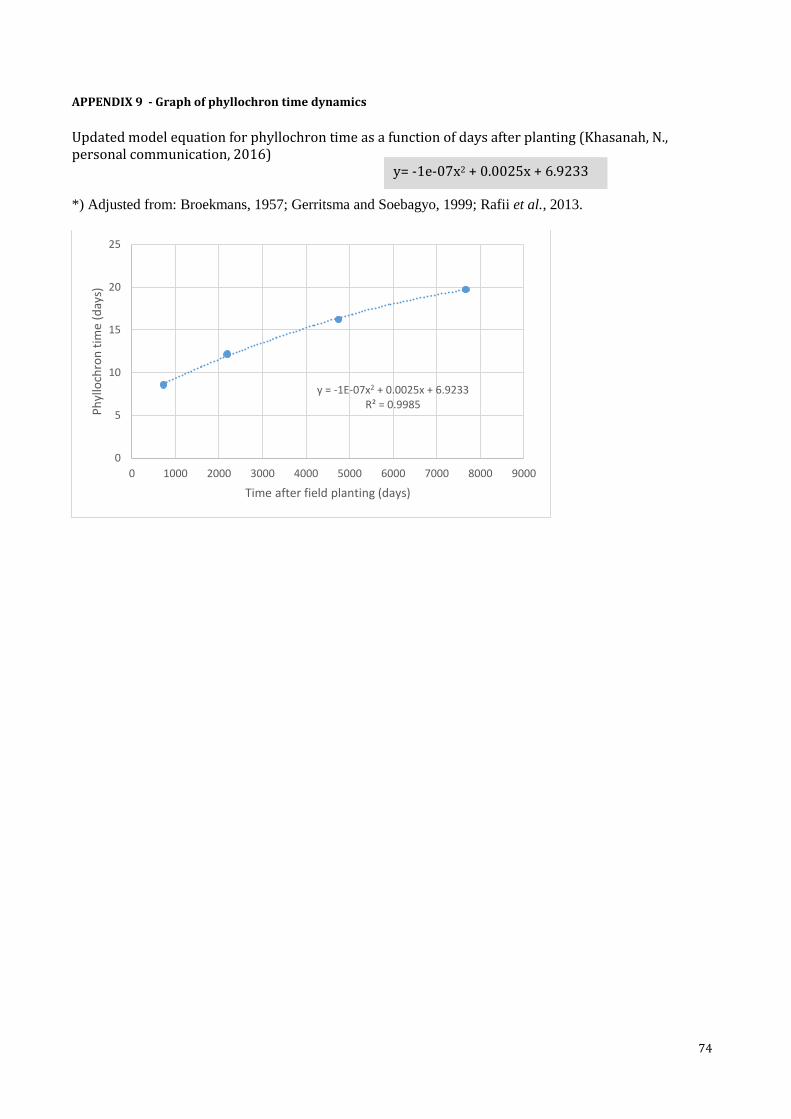
74
APPENDIX 9 - Graph of phyllochron time dynamics
Updated model equation for phyllochron time as a function of days after planting (Khasanah, N., personal communication, 2016)
*) Adjusted from: Broekmans, 1957; Gerritsma and Soebagyo, 1999; Rafii et al., 2013.
y = -1E-07x2 + 0.0025x + 6.9233 R² = 0.9985
0
5
10
15
20
25
0 1000 2000 3000 4000 5000 6000 7000 8000 9000
Ph
yllo
chro
n t
ime
(day
s)
Time after field planting (days)
y= -1e-07x2 + 0.0025x + 6.9233

75
APPENDIX 10 – Two examples of performance variability over drought and soil
Average erosion rate (g/ha/yr) for the 25-year cycle, for the monoculture and cacao and rubber
intercrop systems. On the Y-axis the 4 combinations of drought (15 or 60 days consecutive per year)
and soil (sandy loam = SL, or clay loam = CL). The graph shows that cacao has reduced erosion levels
for the sandy loam soil, but increased levels for the clay loam soils.
Net present value at year 25. On the Y-axis the 4 combinations of drought (15 or 60 days consecutive
per year) and soil (sandy loam = SL, or clay loam = CL). The graph shows that the performance of the
mucuna ground cover scenario is very similar to the performance of the oil palm monoculture. For SL
the mucuna obtained a larger NPV whereas for the clay loam oil palm obtained a larger NPV.

76
APPENDIX 11 – Profitability module input
Perennial module: labour requirements, seed costs and tree product prices in Indonesian Rupiah (1 Rp. = 6.83*10-5
EURO, exchange rate 01/10/2016, XE currency 2016)
Oil palm1 Cacao Rubber
Labour for planting (person days per tree) 0.126 0.126 0.178
Labour for pruning (person days per kg) 0.000405 0.02 -
Labour for fruit harvest (person days per kg) 0.00113 0.07 -
Labour for latex harvest (person days per kg) - - 0.115
Labour for fertilizer application (person days per ha) 4.5 2 1.5
Seed cost (Rp. per tree) 8000 1000 3000
Fruit price (Rp. per kg)2 1400 26000 -
Latex price (Rp. per kg) 3 - - 4485
Annual module: labour requirements (per cropping season), seed costs and crop yield prices in Indonesian Rupiah (1
Rp. = 6.83*10-5 EURO, exchange rate 01/10/2016, XE currency 2016).
Mucuna Cassava Groundnut
Labour for planting (person days per ha) 2 10 14.5
Labour for weeding (person days per ha) 2 20 12
Labour for harvesting (person days per Mg) - 10 20
Labour for fertilizer application (person days per ha) - 1.5 1.5
Seed cost (Rp. per kg) 2000 3000 20000
Yield price (Rp. per kg) 4 - 900 3500
1 Labour inputs based on: Corley & Tinker (2015), Table 11.6 p. 300 2 FaoStat 10 year average Indonesia 3 FaoStat 10 year average Indonesia 4 FaoStat 10 year average Indonesia

77
APPENDIX 12- Spatial levels of importance and linked stakeholders
As explained oil palm cultivation is part of a complex system of interests from multiple stakeholders,
which are acting at different spatial levels.
At a first level is the smallholder, addressed in the previous sections. At a second level are the
local communities in which these smallholders and agribusinesses act. For this stakeholder the largest
concern are: increased risk of flooding, water quality deterioration, reduced food security and food
sovereignty (Colchester, 2011; Obidzinski et al., 2012). The local and regional authorities are
concerned with these issues, but also with the economic implications of oil palm and economic
vulnerability of the region. Then there is a stakeholder, for this study simplified to ‘External’: including
NGOs and food manufacturers, which focus on increasing the image of oil palm sustainability
(McCarthy, 2010; Silva-Castañeda, 2012).

78
APPENDIX 13- Annual cumulative yield per cropping scenario over the 25-year simulation
The annual and cumulative simulated yields for the monoculture and intercropping scenarios in dry weight per hectare. The values are the average of the four productivity level for the soil and drought conditions. OPF = Oil palm fruit.
OPF (kg dm/ha)
OPF (kg dm/ha)
Cocoa pod (kg dm/ha)
OPF (kg dm/ha)
Latex (kg dm/ha)
OPF (kg dm/ha)
OPF (kg dm/ha)
Groundnut (kg dm/ha)
OPF (kg dm/ha)
Cassava kg dm/ha
year Oil palm mono
Oil palm +Cacao
Oil palm +Rubber
Oil palm +Mucuna
Oil palm +Groundnut
Oil palm +Cassava
1 0 0 0 0 0 0 0 4.1 0 6.6
2 0.1 0.2 0 0 0 0.1 0 4.1 0 6.3
3 0.2 0.4 0 0.2 0 0.2 0.2 1.7 0.2 0
4 0.6 0.7 0 0.3 0 0.6 0.6 0 0.4 0
5 0.8 0.8 0 0.4 0 0.8 0.9 0 0.7 0
6 0.9 0.9 0.1 0.3 0.1 1.1 1 0 1 0
7 1.1 1 0 0.3 0 1.1 1.3 0 1.1 0
8 1.3 1 0.1 0.4 0.1 1.4 1.3 0 1.4 0
9 1.5 1.2 0 0.5 0.1 1.4 1.5 0 1.4 0
10 1.5 1.2 0 0.5 0 1.5 1.5 0 1.5 0
11 1.5 1.2 0.1 0.6 0.1 1.5 1.5 0 1.6 0
12 1.6 1.2 0 0.7 0.1 1.7 1.7 0 1.6 0
13 1.7 1.3 0.1 0.7 0.1 1.6 1.5 0 1.6 0
14 1.6 1.4 0 0.6 0.1 1.6 1.6 0 1.7 0
15 1.6 1.4 0.1 0.7 0.2 1.7 1.7 0 1.7 0
16 1.7 1.3 0 0.7 0.1 1.6 1.7 0 1.6 0
17 1.5 1.2 0.1 0.8 0.1 1.6 1.5 0 1.5 0
18 1.5 1.3 0 0.6 0.1 1.5 1.5 0 1.6 0
19 1.5 1.3 0.1 0.7 0.2 1.5 1.5 0 1.5 0
20 1.5 1.1 0 0.7 0.1 1.5 1.5 0 1.5 0
21 1.4 1.2 0.1 0.7 0.2 1.4 1.4 0 1.5 0
22 1.5 1.1 0 0.6 0.1 1.4 1.4 0 1.4 0
23 1.3 1.1 0.1 0.7 0.2 1.4 1.4 0 1.4 0
24 1.3 1.1 0 0.6 0.1 1.3 1.3 0 1.3 0
25 1.3 1 0 0.7 0.2 1.3 1.2 0 1.3 0
CUM 30.5 25.6 0.9 13 2.3 30.8 30.7 9.9 30.5 12.9