Soil Moisture Active Passive (SMAP)

Algorithm Theoretical Basis Document (ATBD)

SMAP Level 3 Radar Freeze/Thaw Data Product (L3_FT_A) Initial Release, v.1 Kyle McDonald, Erika Podest, Scott Dunbar, Eni Njoku Jet Propulsion Laboratory California Institute of Technology Pasadena, CA John Kimball Flathead Lake Biological Station University of Montana Polson, MT Jet Propulsion Laboratory California Institute of Technology

© 2012. All rights reserved.

2

(Page intentionally left blank)

3

Algorithm Theoretical Basis Documents (ATBDs) provide the physical and mathematical descriptions of the algorithms used in the generation of science data products. The ATBDs include a description of variance and uncertainty estimates and considerations of calibration and validation, exception control and diagnostics. Internal and external data flows are also described.

The SMAP ATBDs were reviewed by a NASA Headquarters review panel in January 2012 and are currently at Initial Release, version 1. The ATBDs will undergo additional updates after the SMAP Algorithm Review in September 2013.

4

Table of Contents

ACRONYMS AND ABBREVIATIONS ..................................................................................... 5  1 INTRODUCTION .................................................................................................................. 6

1.1 THE SOIL MOISTURE ACTIVE PASSIVE (SMAP) MISSION ................................................... 6 1.1.1 BACKGROUND AND SCIENCE OBJECTIVES .................................................................... 6 1.1.2   MEASUREMENT APPROACH .......................................................................................... 6  

1.2   SMAP REQUIREMENTS RELATED TO FREEZE-THAW STATE ............................................... 9  2   BACKGROUND AND HISTORICAL PERSPECTIVE .................................................. 10  

2.1   PRODUCT/ALGORITHM OBJECTIVES .................................................................................. 11  2.2   L3_FT_A PRODUCTION .................................................................................................... 12  2.3   DATA PRODUCT CHARACTERISTICS .................................................................................. 14  

3   PHYSICS OF THE PROBLEM .......................................................................................... 16  3.1   SYSTEM MODEL ................................................................................................................ 16  3.2   RADIATIVE TRANSFER AND BACKSCATTER ....................................................................... 17  

4   RETRIEVAL ALGORITHM .............................................................................................. 18  4.1   THEORETICAL DESCRIPTION ............................................................................................. 18  

4.1.1   BASELINE AND OPTIONAL ALGORITHMS .................................................................... 18  4.1.2   VARIANCE AND UNCERTAINTY ESTIMATES ................................................................ 20  

4.2   PRACTICAL CONSIDERATIONS ........................................................................................... 22  4.2.1   PROCESSING AND DATA FLOW CONSIDERATIONS ....................................................... 23  4.2.2   ANCILLARY DATA AVAILABILITY/CONTINUITY ......................................................... 23  4.2.3   CALIBRATION AND VALIDATION ................................................................................ 25  4.2.4   TEST PROCEDURES ..................................................................................................... 25  4.2.5   ALGORITHM BASELINE SELECTION ............................................................................ 26  

5   CONSTRAINTS, LIMITATIONS, AND ASSUMPTIONS ............................................. 26  6   REFERENCES ..................................................................................................................... 27  APPENDIX 1: GLOSSARY ..................................................................................................... 30  

5

ACRONYMS AND ABBREVIATIONS ATBD Algorithm theoretical basis document AMSR Advanced Microwave Scanning Radiometer ASF Alaska Satellite Facility ATBD Algorithm Theoretical Basis Document CONUS Continental United States CMIS Conical-scanning Microwave Imager Sounder DAAC Distributed Active Archive Center DCA Dual Channel Algorithm DEM Digital Elevation Model EASE Equal Area Scalable Earth [grid] ECMWF European Center for Medium-Range Weather Forecasting EOS Earth Observing System ESA European Space Agency GEOS Goddard Earth Observing System (model) GMAO Goddard Modeling and Assimilation Office GSFC Goddard Space Flight Center JAXA Japan Aerospace Exploration Agency JPL Jet Propulsion Laboratory LTAN Local Time of Ascending Node LTDN Local Time of Descending Node MODIS MODerate-resolution Imaging Spectroradiometer NCEP National Centers for Environmental Prediction NDVI Normalized Difference Vegetation Index NEE Net ecosystem exchange NPOESS National Polar-Orbiting Environmental Satellite System NPP NPOESS Preparatory Project NSIDC National Snow and Ice Data Center NWP Numerical Weather Prediction OSSE Observing System Simulation Experiment PDF Probability Density Function PGE Product Generation Executable RFI Radio Frequency Interference RVI Radar Vegetation Index SAR Synthetic Aperture Radar SDT (SMAP) Science Definition Team SDS (SMAP) Science Data System SMAP Soil Moisture Active Passive SMOS Soil Moisture Ocean Salinity (mission) SNR Signal to Noise Ratio SRTM Shuttle Radar Topography Mission USGS United States Geological Survey VWC Vegetation Water Content

6

1 INTRODUCTION This document provides a complete description of the algorithm used to generate the SMAP

Level 3 land surface freeze/thaw product, including the physical basis, theoretical description and practical considerations for implementing the algorithm. The L3_FT_A product provides a daily classification of freeze/thaw state derived from the SMAP high-resolution radar output to 3 km polar and global EASE grids. Details of the algorithm implementation and validation approach for the SMAP L3_FT_A terrestrial freeze-thaw state data product are included.

1.1 THE SOIL MOISTURE ACTIVE PASSIVE (SMAP) MISSION

1.1.1 BACKGROUND AND SCIENCE OBJECTIVES The National Research Council’s (NRC) Decadal Survey, Earth Science and Applications

from Space: National Imperatives for the Next Decade and Beyond, was released in 2007 after a two year study commissioned by NASA, NOAA, and USGS to provide them with prioritization recommendations for space-based Earth observation programs [National Research Council, 2007]. Factors including scientific value, societal benefit and technical maturity of mission concepts were considered as criteria. SMAP data products have high science value and provide data towards improving many natural hazards applications. Furthermore SMAP draws on the significant design and risk-reduction heritage of the Hydrosphere State (Hydros) mission [Entekhabi et al., 2004]. For these reasons, the NRC report placed SMAP in the first tier of missions in its survey. In 2008 NASA announced the formation of the SMAP project as a joint effort of NASA’s Jet Propulsion Laboratory (JPL) and Goddard Space Flight Center (GSFC), with project management responsibilities at JPL. The target launch date is October 2014 [Entekhabi et al., 2010].

The SMAP science and applications objectives are to:

• Understand processes that link the terrestrial water, energy and carbon cycles; • Estimate global water and energy fluxes at the land surface; • Quantify net carbon flux in boreal landscapes; • Enhance weather and climate forecast skill; • Develop improved flood prediction and drought monitoring capability.

1.1.2 MEASUREMENT APPROACH Table 1 is a summary of the SMAP instrument functional requirements derived from its

science measurement needs. The goal is to combine the attributes of the radar and radiometer observations (in terms of their spatial resolution and sensitivity to soil moisture, surface roughness, and vegetation) to estimate soil moisture at a resolution of 10 km, and freeze-thaw state at a resolution of 3 km.

7

Table 1. SMAP Mission Requirements

Scientific Measurement Requirements Instrument Functional Requirements Soil Moisture: ~±0.04 m3m-3 volumetric accuracy(1-sigma) in the top 5 cm for vegetation water content ≤ 5 kg m-2; Hydrometeorology at ~10 km resolution; Hydroclimatology at ~40 km resolution

L-Band Radiometer (1.41 GHz): Polarization: V, H, T3 and T4 Resolution: 40 km Radiometric Uncertainty*: 1.3 K L-Band Radar (1.26 and 1.29 GHz): Polarization: VV, HH, HV (or VH) Resolution: 10 km Relative accuracy*: 0.5 dB (VV and HH) Constant incidence angle** between 35° and 50°

Freeze/Thaw State: Capture freeze/thaw state transitions in integrated vegetation-soil continuum with two-day precision, at the spatial scale of landscape variability (~3 km).

L-Band Radar (1.26 GHz and 1.29 GHz): Polarization: Total Power (HH+VV+HV) Resolution: 3 km Relative accuracy*: 0.7 dB (1 dB per channel if 2 channels are used) Constant incidence angle** between 35° and 50°

Sample diurnal cycle at consistent time of day (6am/6pm Equator crossing); Global, ~3 day (or better) revisit; Boreal, ~2 day (or better) revisit

Swath Width: ~1000 km Minimize Faraday rotation (degradation factor at L-band)

Observation over minimum of three annual cycles Baseline three-year mission life * Includes precision and calibration stability ** Defined without regard to local topographic variation

The SMAP spacecraft is designed for a 685-km circular, sun-synchronous orbit, with equator

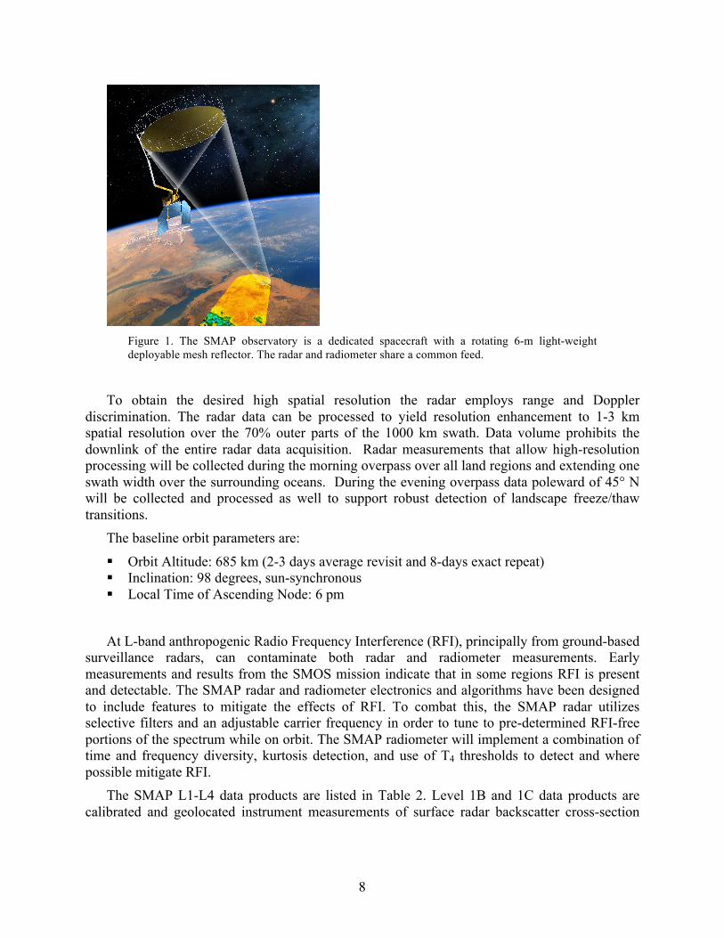
crossings at 6 AM and 6 PM local time. The instrument combines radar and radiometer subsystems that share a single feedhorn and parabolic mesh reflector (Fig. 1). The radar operates with VV, HH, and HV transmit-receive polarizations, and uses separate transmit frequencies for the H (1.26 GHz) and V (1.29 GHz) polarizations. The radiometer operates with polarizations V, H, and the third and fourth Stokes parameters, T3, and T4, at 1.41 GHz. The T3-channel measurement is used to assist in the correction of Faraday rotation effects. The reflector is offset from nadir and rotates about the nadir axis at 14.6 rpm, providing a conically scanning antenna beam at a surface incidence angle of approximately 40°. The provision of constant incidence angle across the swath simplifies the data processing and enables accurate repeat-pass estimation of soil moisture and freeze/thaw change. The reflector diameter is 6 m, providing a radiometer footprint of approximately 40 km (root-ellipsoidal area) defined by the one-way 3-dB beamwidth. The two-way 3-dB beamwidth defines the real-aperture radar footprint of approximately 30 km. The real-aperture (‘lo-res’) swath width of 1000 km provides global coverage within 3 days or less equatorward of 35°N and 2 days poleward of 55°N. The real-aperture radar and radiometer data will be collected globally during both ascending and descending passes.

8

Figure 1. The SMAP observatory is a dedicated spacecraft with a rotating 6-m light-weight deployable mesh reflector. The radar and radiometer share a common feed.

To obtain the desired high spatial resolution the radar employs range and Doppler

discrimination. The radar data can be processed to yield resolution enhancement to 1-3 km spatial resolution over the 70% outer parts of the 1000 km swath. Data volume prohibits the downlink of the entire radar data acquisition. Radar measurements that allow high-resolution processing will be collected during the morning overpass over all land regions and extending one swath width over the surrounding oceans. During the evening overpass data poleward of 45° N will be collected and processed as well to support robust detection of landscape freeze/thaw transitions.

The baseline orbit parameters are:

Orbit Altitude: 685 km (2-3 days average revisit and 8-days exact repeat) Inclination: 98 degrees, sun-synchronous Local Time of Ascending Node: 6 pm

At L-band anthropogenic Radio Frequency Interference (RFI), principally from ground-based surveillance radars, can contaminate both radar and radiometer measurements. Early measurements and results from the SMOS mission indicate that in some regions RFI is present and detectable. The SMAP radar and radiometer electronics and algorithms have been designed to include features to mitigate the effects of RFI. To combat this, the SMAP radar utilizes selective filters and an adjustable carrier frequency in order to tune to pre-determined RFI-free portions of the spectrum while on orbit. The SMAP radiometer will implement a combination of time and frequency diversity, kurtosis detection, and use of T4 thresholds to detect and where possible mitigate RFI.

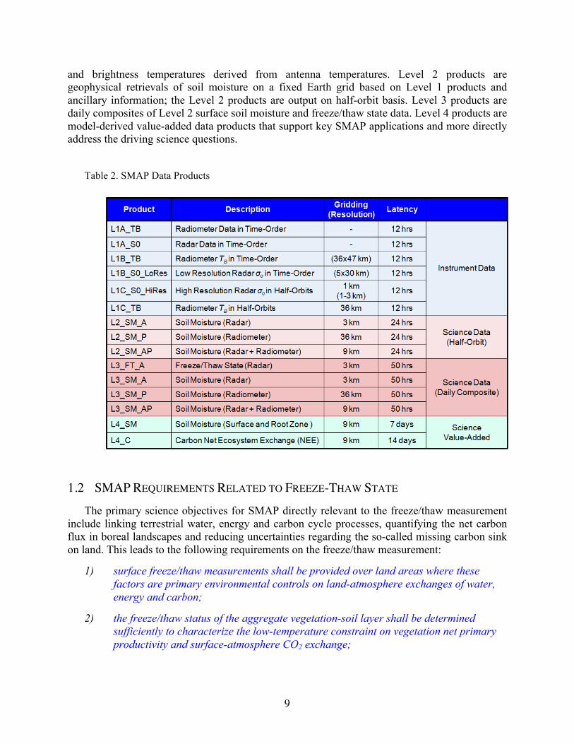
The SMAP L1-L4 data products are listed in Table 2. Level 1B and 1C data products are calibrated and geolocated instrument measurements of surface radar backscatter cross-section

9

and brightness temperatures derived from antenna temperatures. Level 2 products are geophysical retrievals of soil moisture on a fixed Earth grid based on Level 1 products and ancillary information; the Level 2 products are output on half-orbit basis. Level 3 products are daily composites of Level 2 surface soil moisture and freeze/thaw state data. Level 4 products are model-derived value-added data products that support key SMAP applications and more directly address the driving science questions.

Table 2. SMAP Data Products

1.2 SMAP REQUIREMENTS RELATED TO FREEZE-THAW STATE

The primary science objectives for SMAP directly relevant to the freeze/thaw measurement include linking terrestrial water, energy and carbon cycle processes, quantifying the net carbon flux in boreal landscapes and reducing uncertainties regarding the so-called missing carbon sink on land. This leads to the following requirements on the freeze/thaw measurement:

1) surface freeze/thaw measurements shall be provided over land areas where these factors are primary environmental controls on land-atmosphere exchanges of water, energy and carbon;

2) the freeze/thaw status of the aggregate vegetation-soil layer shall be determined sufficiently to characterize the low-temperature constraint on vegetation net primary productivity and surface-atmosphere CO2 exchange;

10

3) SMAP shall measure landscape freeze/thaw with a spatial resolution of 3 km;

4) SMAP shall measure landscape freeze/thaw with a mean temporal sampling of 2 days or better;

5) SMAP shall measure freeze/thaw with accuracy sufficient to resolve the temporal dynamics of net ecosystem exchange to within 0.05 tons C ha-1 (or 3%) over a ~100-day growing season.

Current SMAP baseline mission requirements specific to terrestrial freeze-thaw science activities state that:

[Level 1 mission requirement] The baseline science mission shall provide estimates of surface binary freeze/thaw state in the region north of 45° N latitude, which includes the boreal forest zone, with a classification accuracy of 80% at 3 km spatial resolution and 2-day average intervals.

The above requirements form the basis of the design of the L3_FT_A product. This document includes descriptions of baseline and optional freeze/thaw state classification algorithms, and discussion of theoretical assumptions and procedures for refining and testing the algorithms to achieve these mission requirements.

2 BACKGROUND AND HISTORICAL PERSPECTIVE

The terrestrial cryosphere comprises cold areas of Earth's land surface where water is either permanently or seasonally frozen. This includes most regions north of 45°N latitude and most areas with elevation greater than 1000 meters. Within the terrestrial cryosphere, spatial patterns and timing of landscape freeze-thaw state transitions are highly variable with measurable impacts to climate, hydrological, ecological and biogeochemical processes.

Landscape freeze/thaw state influences the seasonal amplitude and partitioning of surface energy exchange strongly, with major consequences for atmospheric profile development and regional weather patterns (Betts et al., 2000a). In seasonally frozen environments, ecosystem responses to seasonal thaw are rapid, with soil respiration and plant photosynthetic activity accelerating with warmer temperatures and the abundance of liquid water (e.g., Goulden et al., 1998; Black et al., 2000; Jarvis and Linder, 2000). The timing of seasonal freeze/thaw transitions generally defines the duration of seasonal snow cover, frozen soils, and the timing of lake and river ice breakup and flooding in the spring (Kimball et al., 2001, 2004a). The seasonal non-frozen period also bounds the vegetation growing season, while annual variability in freeze/thaw timing has a direct impact on net primary production and net ecosystem CO2 exchange (NEE) with the atmosphere (Vaganov et al., 1999; Goulden et al., 1998).

Satellite-borne microwave remote sensing has unique capabilities that allow near real-time monitoring of numerous landscape processes associated with a single measure, freeze/thaw state, without many of the limitations of optical-infrared sensors such as solar illumination or atmospheric conditions. The SMAP L3_FT_A product is designed to provide the most accurate

11

remote sensing-based characterization of landscape freeze-thaw state available at global scale. The unique design of the SMAP L-band radar allows a combined spatial and temporal characterization of terrestrial freeze-thaw transitions previously unavailable.

The SMAP L3_FT_A baseline and optional algorithms follow from an extensive heritage of previous work, initially involving truck mounted radar scatterometer and radiometer studies over bare soils and croplands (Ulaby et al., 1986; Wegmuller, 1990), followed by aircraft SAR campaigns over boreal landscapes (Way et al., 1990), and subsequently from a variety of satellite-based SAR, radiometer and scatterometer studies at regional, continental and global scales (Rignot and Way, 1994; Rignot et al., 1994; Way et al., 1997; Frolking et al., 1999; Wisman, 2000; Kimball et al., 2001; 2004a,b; McDonald et al., 2004; Rawlins et al., 2005; Kim et al., 2010; Podest, 2006). These investigations have included regional, pan-boreal, and global scale efforts, supporting development of retrieval algorithms, assessment of applications of remotely sensed freeze/thaw state for supporting ecologic and hydrological studies, and more recently in assembly of a global-scale Earth System Data Record (ESDR) developed from SSM/I and now in distribution at the National Snow and Ice Center (Kim, et al., 2010). The SSM/I ESDR is the first of its kind, providing daily freeze-thaw state across multiple years and including delineation of AM/PM freeze/thaw transitional states.

The L3_FT_A baseline and optional algorithms classify the land surface freeze/thaw state based on the time series radar backscatter response to the change in dielectric constant of the land surface components associated with water transitioning between solid and liquid phases. This response dominates the seasonal pattern of radar backscatter for regions of the global land surface undergoing seasonal freeze-thaw transitions. The timing of the springtime freeze-thaw state transitions corresponding to this radar backscatter response coincides with the timing of growing season initiation in boreal, alpine and arctic tundra regions of the global cryosphere. Interannual variability in these processes is a major control on annual vegetation productivity and land-atmosphere CO2 exchange (Frolking et al., 1999; Kimball et al., 2004; McDonald et al., 2004). Thus the L3_FT_A algorithm supports characterization of the spatial and temporal dynamics of landscape freeze-thaw state for regions of the global land surface where cold temperatures are limiting for photosynthesis and respiration processes and where the timing and variability in landscape freeze-thaw processes have an associated key impact on vegetation productivity and the carbon cycle.

2.1 PRODUCT/ALGORITHM OBJECTIVES

Figure 2 shows the data sets associated with L3_FT_A product generation, including input and output data. There is one primary SMAP freeze/thaw product. The L3_FT_A product consists of daily composite landscape freeze/thaw state derived from global AM (descending) pass radar data stream (L1C_S0_HiRes half-orbits) and north of 45°N, the ascending PM pass data. The L1C_S0_HiRes AM data will also be utilized to generate a freeze/thaw binary state flag for use in the L2/3_SM product algorithms. The L3_FT_A product is gridded and provided on a 3 km Equal Area Scalable Earth grid (EASE-grid) in both global and north polar projections.

12

The baseline L3_FT_A product is designed to fulfill the SMAP mission freeze-thaw science requirements summarized in Section 1 above. The baseline product provides freeze-thaw state classification information with an inherent spatial resolution of 3 km with temporal revisit of 2 days or better north of 45°N and 3 days or better elsewhere. The data product will be global in extent, covering unmasked regions of Earth’s land mass where low temperatures are a significant constraint to vegetation productivity and terrestrial carbon exchange (Churkina and Running, 2000; Nemani et al., 2003; Kim et al., 2010). Product accuracy associated with meeting SMAP mission requirements will be met for the product domain north of 45°N latitude. Accuracy of the product for the full freeze/thaw domain including regions south of 45°N will be assessed and provided as part of SMAP cal/val activities.

Freeze/thaw state will be generated separately for AM and PM radar acquisitions. Combining SMAP freeze/thaw state assessments from AM and PM acquisitions provides unique information on regions undergoing freeze/thaw transitions on a diurnal basis (e.g. Kim et al., 2010). This aspect of the product supports enhanced investigation of spring and autumn transition seasons and the associated controls on annual vegetation productivity. The L1C_S0_HiRes PM data will be used to support generation of this product for regions north of 45°N latitude, as a standard deliverable product. Options for utilizing L1B_S0_LoRes PM radar data for regions south of 45°N will be explored as a research component of the L3_FT_A product.

The radar freeze-thaw algorithm will also supply a 3km resolution AM global binary freeze/thaw state flag as an intermediate output product to be utilized within the L2_SM_A radar soil moisture processing to identify frozen land regions, and in that context supporting the generation of the L2 and L3 active, passive, and active-passive products (L2/3_SM_A, L2/3_SM_P, L2/3_SM_AP).

2.2 L3_FT_A PRODUCTION

Production of the L3_FT_A data sets will be carried out at JPL during SMAP mission operations. An overview of the L3_FT_A processing sequence is provided in Figure 2. Research using SSM/I radiometer and SeaWinds-on-QuikSCAT scatterometer data indicate substantial variability of freeze/thaw spatial and temporal dynamics derived from AM and PM overpass data with important linkages to surface energy balance and carbon cycle dynamics (McDonald and Kimball, 2005; Kim et al., 2010). L3_FT_A algorithm products generated utilizing both ascending (PM) and descending (AM) radar backscatter data streams will enable regional assessment and monitoring of diurnal variability in terrestrial freeze/thaw state dynamics.

SMAP mission specifications provide for collection of high resolution (3 km) radar backscatter (L1C_S0_HiRes) for descending orbits (6 AM overpass) over land and for that portion of ascending orbits (6 PM overpass) over land north of 45°N latitude. Low (~5x30 km) resolution radar data (L1B_S0_LoRes) provides global coverage for AM and PM overpass orbits. These radar backscatter data streams will provide calibrated and geolocated σo data, with L1B_S0_LoRes in time order and L1C_S0_HiRes in individual half-orbit files. The L3_FT_A product will utilize the L1C_S0_HiRes data stream for standard production. The use of L1B_S0_LoRes radar backscatter data will be explored in a research context supporting provision of a diurnal component to the L3_FT_A product south of 45°N.

13

The L3_FT_A algorithm will be applied to the radar data granules for unmasked land regions. The resulting intermediate freeze-thaw products (Figure 2) will serve two purposes: (1) these data will be assembled into global daily composites in production of the L3_FT_A product, and (2) the freeze/thaw product derived from global AM L1C_S0_HiRes granules will provide the binary freeze/thaw state flag supporting generation of the L2 and L3 soil moisture products.

Figure 2. Processing sequence for generation of the L3_FT_A product and the binary freeze/thaw state

flag to be used in generation of the SMAP soil moisture products.

The L3_FT_A algorithm is applied to the total power radar data streams, total power being the sum of HH, VV, and HV polarized backscatter. This provides the best signal-to-noise characteristic from the SMAP radar, thus optimizing product accuracy. The L3_FT_A algorithms may also be employed to produce landscape freeze/thaw state information from SMAP L1C_TB brightness temperature observations. Hence in the event of a failure of the SMAP radar data stream, freeze-thaw data products could be produced using the L1C_TB data stream, but at a lower (~40 km) spatial resolution at the grid posting of 36 km of the L1C_TB product.

Radar freeze/thaw data processing will occur over unmasked portions of the global land surface domain. In addition, the freeze/thaw retrieval will take into account the transient open water flag determined from the 3 km gridded backscatter in the L2_SM_A processing. No L3_FT_A data processing will occur over masked areas. It is anticipated that “no-data” flags will be associated with L3_FT_A product identifying each of the masked surface types: ocean and inland open water (static and transient), permanent ice and snow, and urban areas. The L3_FT_A algorithms do not utilize ancillary data during execution and processing. However, ancillary data will be utilized extensively to initialize the state change thresholds that are employed in the baseline algorithm change detection scheme. Although not strictly required, prior initialization of

14

these thresholds enhances algorithm efficiency and accuracy. Ancillary data planned for use in generation of the L3_FT_A product are summarized in Section 4.

2.3 DATA PRODUCT CHARACTERISTICS

The L3_FT_A product will delineate freeze/thaw state on a pixel-wise basis according to the nomenclature in Table 4. An example of this product derived from SSM/I brightness temperature data utilizing the baseline L3_FT_A algorithm is shown in Figure 3. The global scale domain shown in Figure 3 corresponds to those regions of Earth’s land surface where low temperatures are a significant constraint to vegetation productivity and terrestrial carbon exchange (Churkina and Running, 2000; Nemani et al., 2003; Kim et al, 2010). The delineation of this domain is a subject of on-going research and may be updated prior to SMAP operations pending research outcomes.

Table 4. Nomenclature of the SMAP L3_FT_A product, indicating the landscape state as observed during AM and PM overpasses, and the corresponding freeze/thaw classification terminology. The AM overpass state will be provided at 3 km spatial resolution. The PM overpass data will be at 3 km resolution for regions north of 45°N and 5x30 km resolution otherwise. Those product components utilizing the low resolution (5x30 km) data stream are considered research products.

Landscape State F/T Classification Terminology combining

AM and PM data AM Overpass PM Overpass

Frozen Frozen Frozen Thawed Thawed Thawed Frozen Thawed Transitional Thawed Frozen Inverse Transitional

Table 5. Spatial resolution of the components of the L3_FT_A product based on AM and PM

radar acquisitions. Those product components utilizing the low resolution (5x30 km) data stream are considered research products.

Region AM Overpass

PM Overpass

AM+PM Combined

North of 45°N lat 3 km 3 km 3 km

South of 45°N lat 3 km 5x30 km(1)

5x30 km(1)

(1) Components of the L3_FT_A product to be considered for research products

15

Figure 3. Example of a global daily freeze/thaw product for April 10, 2004 derived from SSM/I (37 GHz channel) at 25 km resolution. Regions of frozen, thawed (here termed “non-frozen), transitional and inverse-transitional are identified. The global-scale domain of this map corresponds to those regions of Earth’s land surface where cold temperatures are a significant constraint to vegetation productivity,

Radar backscatter observations are acquired for the global land surface at 3 km resolution (L1C_S0_HiRes) for the AM (descending) orbital nodes. For the PM (ascending) orbital nodes, high-resolution backscatter (L1C_S0_HiRes) is acquired at 3 km resolution for regions north of 45°N latitude. Low-resolution radar (L1B_S0_LoRes) data at 5x30 km will be available for regions south of 45°N latitude on the PM passes. The resulting combined product will use both AM and PM data in combination to delineate frozen, thawed, transitional and inverse transitional conditions. The AM overpass landscape state is provided at 3 km resolution everywhere in the L3_FT_A product domain. The PM overpass landscape state is provided at 3 km resolution north of 45°N latitude (baseline product) and at 5x30 km elsewhere (research product). The L3_FT_A product will include the 3 km AM product for the global-scale domain, the 3 km PM product for the region north of 45°N, and may include the 5x30 km product south of 45°N as a research product (Table 4). All renderings are posted to a 3 km EASE-Grid, both in global and north polar projections.

The L3_FT_A algorithm will be applied to regridded L1C_S0_HiRes radar data as a baseline (Figure 2). Implementing the L3_FT_A algorithm in this way will ensure production of the binary state freeze/thaw flag consistent with the needs of the L2/L3 soil moisture processing. This intermediate freeze/thaw products will be temporally composited to assemble daily freeze-thaw state maps separately for AM and PM acquisitions. The daily temporal compositing process will be performed on the 3 km EASE grid data, retaining the freeze-thaw state associated with those acquisitions closest to 6:00 AM local time (AM daily product) and 6:00 PM local time (PM daily product). These daily intermediate products will be further composited into multi-day products, keeping the latest date of acquisition as a replacement for acquisitions acquired on older dates, to ensure full coverage of the global scale freeze/thaw domain for AM and PM acquisitions separately. These AM and PM multi-date composites will be used to derive the

16

combined product with nomenclature shown in Table 4 above. The respective date and time of acquisition of each of the AM and PM components of the data stream will be maintained in the data set. The daily L3_FT_A product will thus incorporate AM and PM data for the current day, as well as past days’ information to ensure complete coverage of the global-scale freeze/thaw domain in each day’s product.

Formatting of the L3_FT_A product will be HDF5 with appropriate metadata. The L3_FT_A will be posted to both polar and global equal-area Earth grids. The projections are defined in terms of north polar azimuthal and global cylindrical Equal-Area Scalable Earth (EASE) grids (Armstrong and Brodzik, 1995). These gridding schemes are similar to current postings of the SSM/I.

Latency is defined as the average time under normal operating conditions between data acquisition by the SMAP observatory and delivery of the product to the data center. Latency of the baseline L3_FT_A product is dependent on the delivery rate of L1C_S0_HiRes (47 GB per day) data from the radar processing system and on the rate at which these can be processed into freeze/thaw products and submitted to the SMAP NSIDC DAAC. Processing of the baseline L3_FT_A product will be complete within 24 hours of receipt of the global L1C_S0_HiRes data, which itself has a latency of 12 hours. Latencies associated with the optional algorithms are significantly longer, as these algorithms involve the analysis of seasonal patterns in L1C_S0_HiRes daily time series data. The optional algorithms will likely involve data collection and latency intervals from 6-months to 1-year.

3 PHYSICS OF THE PROBLEM 3.1 SYSTEM MODEL

The ability of microwave remote sensing instruments to observe freezing and thawing of a landscape has its origin in the distinct changes of surface dielectric properties that occur as water transitions between solid and liquid phases. A material’s permittivity describes how that material responds in the presence of an electromagnetic field (Kraszewski, 1996). As an electromagnetic field interacts with a dielectric material, the resulting displacement of charged particles from their equilibrium positions gives rise to induced dipoles that respond to the applied field. A material’s permittivity is a complex quantity (i.e., having both real and imaginary numerical components) expressed as: ' ''jε ε ε= − (1)

and is often normalized to the permittivity of a vacuum (ε0) and referred to as the relative permittivity, or the complex dielectric constant: 0 0'/ ''/ ' ''.r r rj jε ε ε ε ε ε ε= − = − (2)

The real component of the dielectric constant, 'rε , is related to a material’s ability to store electric field energy. The imaginary component of the dielectric constant, ''rε , is related to the dissipation or energy loss within the material. At microwave wavelengths, the dominant

17

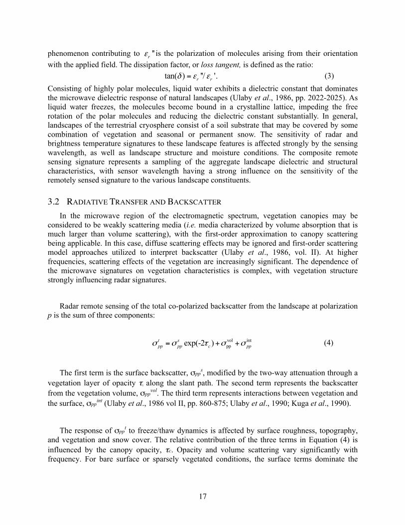
phenomenon contributing to ''rε is the polarization of molecules arising from their orientation with the applied field. The dissipation factor, or loss tangent, is defined as the ratio: tan( ) ''/ '.r rδ ε ε= (3) Consisting of highly polar molecules, liquid water exhibits a dielectric constant that dominates the microwave dielectric response of natural landscapes (Ulaby et al., 1986, pp. 2022-2025). As liquid water freezes, the molecules become bound in a crystalline lattice, impeding the free rotation of the polar molecules and reducing the dielectric constant substantially. In general, landscapes of the terrestrial cryosphere consist of a soil substrate that may be covered by some combination of vegetation and seasonal or permanent snow. The sensitivity of radar and brightness temperature signatures to these landscape features is affected strongly by the sensing wavelength, as well as landscape structure and moisture conditions. The composite remote sensing signature represents a sampling of the aggregate landscape dielectric and structural characteristics, with sensor wavelength having a strong influence on the sensitivity of the remotely sensed signature to the various landscape constituents. 3.2 RADIATIVE TRANSFER AND BACKSCATTER

In the microwave region of the electromagnetic spectrum, vegetation canopies may be considered to be weakly scattering media (i.e. media characterized by volume absorption that is much larger than volume scattering), with the first-order approximation to canopy scattering being applicable. In this case, diffuse scattering effects may be ignored and first-order scattering model approaches utilized to interpret backscatter (Ulaby et al., 1986, vol. II). At higher frequencies, scattering effects of the vegetation are increasingly significant. The dependence of the microwave signatures on vegetation characteristics is complex, with vegetation structure strongly influencing radar signatures.

Radar remote sensing of the total co-polarized backscatter from the landscape at polarization p is the sum of three components:

vol intppexp(-2 )t s

pp pp c ppσ σ τ σ σ= + + (4)

The first term is the surface backscatter, σpps, modified by the two-way attenuation through a

vegetation layer of opacity τc along the slant path. The second term represents the backscatter from the vegetation volume, σpp

vol. The third term represents interactions between vegetation and the surface, σpp

int (Ulaby et al., 1986 vol II, pp. 860-875; Ulaby et al., 1990; Kuga et al., 1990).

The response of σppt to freeze/thaw dynamics is affected by surface roughness, topography,

and vegetation and snow cover. The relative contribution of the three terms in Equation (4) is influenced by the canopy opacity, τc. Opacity and volume scattering vary significantly with frequency. For bare surface or sparsely vegetated conditions, the surface terms dominate the

18

received signal, with σppt being influenced primarily by contributions from the soil surface and

snow cover. Because of the high dielectric constant of liquid water, microwave penetration of the vegetation decreases as biomass moisture levels increase. In general, τc increases with increasing frequency, vegetation density, and dielectric constant. High frequency, short wavelength energy (e.g. Ku-band) has higher τc and does not penetrate as significantly into vegetation canopies as lower frequency, longer wavelength energy (e.g. L-band). Hence, lower frequency sensors are generally more sensitive to properties of surfaces underlying dense vegetation canopies. However, the dependence of σpp

t on snow characteristics is also complex, with snow pack wetness, density, crystal structure, and depth influencing backscatter. The effect of snow cover on radar backscatter is more significant at higher frequencies owing to the increased scattering albedo of the snow pack at short wavelengths relative to longer wavelengths (e.g., Ulaby et al., 1986; Raney, 1998) These phenomena lead to notable differences in the temporal response of emission and backscatter to landscape freeze/thaw processes with sensor wavelengths (e.g., Way et al., 1994; Way et al., 1997; Frolking et al., 1999; Kimball et al., 2001).

4 RETRIEVAL ALGORITHM 4.1 THEORETICAL DESCRIPTION

Derivation of the SMAP L3_FT_A product will employ a temporal change detection approach that has been previously developed and successfully applied using time-series satellite remote sensing radar backscatter and radiometric brightness temperature data from a variety of sensors and spectral wavelengths. The approach is to identify landscape F/T transition by identifying the temporal response of backscatter or brightness temperature to changes in the dielectric constant of the landscape components that occur as the water within the components transitions between frozen and non-frozen conditions. Classification algorithms assume that the large changes in dielectric constant occurring between frozen and non-frozen conditions dominate the corresponding backscatter and brightness temperature temporal dynamics across the seasons, rather than other potential sources of temporal variability such as changes in canopy structure and biomass or large precipitation events. This assumption is valid for most areas of the terrestrial cryosphere.

4.1.1 BASELINE AND OPTIONAL ALGORITHMS

Three distinct temporal change detection algorithms have been identified for classification of landscape F/T state using SMAP time-series L-band radar data. The F/T algorithms include a seasonal threshold approach (baseline algorithm), as well as moving window and temporal edge detection algorithms (optional algorithms). Although information from the optional algorithms may eventually prove useful for augmenting the current baseline algorithm, as of this writing no specific plans exist to utilize these algorithms. The algorithms are described in detail below. All of them currently require only time-series radar backscatter information to derive landscape F/T state information. Of the three algorithms only the baseline algorithm provides a daily freeze/thaw state classification that also fulfills the SMAP data latency requirement.

19

SEASONAL THRESHOLD APPROACH (BASELINE ALGORITHM)

The seasonal threshold (baseline) algorithm examines the time series progression of the remote sensing signature relative to signatures acquired during seasonal reference frozen and thawed states. This algorithm is well-suited for application to data with temporally sparse or variable repeat-visit observation intervals and has been applied to ERS and JERS Synthetic Aperture Radar (SAR) imagery (e.g. Rignot and Way, 1994; Way et al., 1997; Gamon et al., 2004; Entekhabi et al., 2004). A seasonal scale factor Δ(t) may be defined for an observation acquired at time t as:

( )

( ) fr

th fr

tt

σ σ

σ σ

−Δ =

− (5)

where σ(t) is the measurement acquired at time t, for which a freeze/thaw classification is sought, and frσ and thσ are backscatter measurements corresponding to the frozen and thawed reference states, respectively. In situations where only a single reference state is available, for example frσ , Δ(t) may be defined as a difference:

( ) ( ) frt tσ σΔ = − (6)

A threshold level T is then defined such that:

( )( )t Tt T

Δ >

Δ ≤ (7)

defines the thawed and frozen landscape states, respectively. This series of algorithms will be run on a cell-by-cell basis for unmasked portions of the domain. The output from Equation (7) will be a dimensionless binary state variable designating either frozen or thawed condition for each unmasked grid cell. Whereas Equation (5) accounts for differences in the dynamic range of the remote sensing response to F/T transitions driven by variations in land cover, Equation (6) does not scale Δ(t) to account for the dynamic range in the seasonal response.

The selection of parameter T may be optimized for various land cover conditions and sensor configurations. In situations where the wintertime microwave signature is not dominated by the snow pack volume, for example for radar measurements at lower frequencies (e.g. L-band) and where shallow dry snowpacks are common, fr thσ σ< and Δ(t) > T defines the thawed state.

A major component of the SMAP baseline algorithm development will involve radar backscatter modeling and application of existing satellite L-band remote sensing data from JERS-1 and ALOS PALSAR over the global terrestrial application area to develop maps of frσ ,

thσ , and T. These activities will be used for calibration and initialization of the F/T threshold algorithms prior to launch. These initial parameters will be evaluated and refined through post-launch reanalysis of the SMAP data stream.

MOVING WINDOW APPROACH (OPTIONAL ALGORITHM) Moving window techniques classify freeze/thaw transitions based on changes in the

radiometric signature relative to the temporally averaged signature computed over a moving

20

window of specified duration. These approaches are useful when applied to temporally consistent data sets consisting of frequent (e.g., daily) observations, and for identifying multiple freeze/thaw transition events. For a measurement σ(t) acquired at time t, the difference δ(t) relative to a moving window mean may be defined as 0( ) ( ) ( 1)avt t t L t tδ σ σ= − − ≤ ≤ − (8)

where 0( 1)av t L t tσ − ≤ ≤ − is the average measurement (backscatter or brightness temperature) acquired over a window of duration L extending over the time interval 0( 1)t L t t− ≤ ≤ − . The difference δ(t) may be compared to various thresholds, as in Eq. (7), to define the timing of critical freeze/thaw transitions. These approaches have been employed using both NSCAT and SeaWinds scatterometer data for a variety of regions (Frolking et al., 1999; Kimball et al., 2001, 2004a,b; Rawlins et al., 2005.) Principal distinctions in the application of Eq. (8) have been the duration L of the moving window and the selection of thresholds applied to infer transition events.

TEMPORAL EDGE DETECTION APPROACH (OPTIONAL ALGORITHM) Temporal edge detection techniques classify freeze/thaw transitions by identifying

pronounced step-edges in time series remote sensing data that correspond to freeze/thaw transition events. As freeze/thaw events induce large changes in landscape dielectric properties that tend to dominate the seasonal time-series response of the microwave radiometric signatures for the terrestrial cryosphere, edge detection approaches are suitable for identification of these events using time-series microwave remote sensing data. These techniques are based on the application of an optimal edge detector for determining edge transitions in noisy signals (Canny, 1986). The timing of a major freeze/thaw event is determined from the convolution applied to a time series of backscatter or brightness temperature measurements σ(t):

( ) '( ) ( )CNV t f x t x dxσ∞

−∞

= −∫ (9)

where f’(x) is the first derivative of a normal (Gaussian) distribution. The occurrence of a step-edge transition is then given by the time when CNV(t) is at a local maximum or minimum.

Seasonal transition periods may involve multiple freeze/thaw events. This technique accounts for the occurrence of weak edges, or less pronounced freeze/thaw events, as well as larger seasonal events indicated by strong edges, and can distinguish the frequencies and relative magnitudes of these events. The variance of the normal distribution may be selected to identify step edges with varying dominance, i.e. selection of a large variance identifies more predominant step edges, while narrower variances allow identification and discrimination of less pronounced events. This approach has been applied to daily time series brightness temperatures from the Special Sensor Microwave/Imager (SSM/I) to map primary springtime thaw events annually across the pan-Arctic basin and Alaska (McDonald et al., 2004).

4.1.2 VARIANCE AND UNCERTAINTY ESTIMATES Refinement and testing of L3_FT_A algorithms will involve utilizing satellite L-band SAR

(e.g., JERS-1 SAR and ALOS PALSAR) and radar backscatter models to assess the simulated

21

SMAP radar backscatter response over a variety of environment, terrain and land cover conditions in order to assess these error sources. Primary sources of error and uncertainty in the freeze/thaw product stems from: (1) radiometric errors due to resolution and sensor viewing geometry (azimuth), (2) geometric errors due to layover and shadowing (slope/aspect), (3) within-season radar backscatter variability not accounted for by the implementation of the constant frozen and thawed reference states employed within the baseline algorithm, and (4) variations in landcover with respect to spatial heterogeneity. Some additional sources are associated with relatively dry landscapes that contain small amounts of water such that changes in freeze/thaw state result in minimal change in backscatter. Also, large precipitation events that significantly wet the land surface such that the additional surface water induces a pronounced backscatter may induce an error in the classified freeze/thaw state. Integrating JERS-1 and PALSAR data sets within the SMAP SDS Testbed will support investigation of system level parameters (e.g. system noise, viewing geometry, and associated topographic effects) in the error and uncertainty assessment.

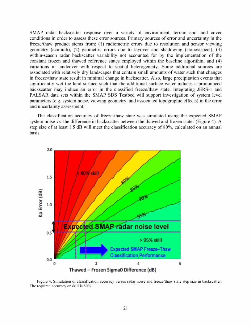
The classification accuracy of freeze-thaw state was simulated using the expected SMAP system noise vs. the difference in backscatter between the thawed and frozen states (Figure 4). A step size of at least 1.5 dB will meet the classification accuracy of 80%, calculated on an annual basis.

Figure 4. Simulation of classification accuracy versus radar noise and freeze/thaw state step size in backscatter.

The required accuracy or skill is 80%.

22

To examine SMAP freeze/thaw algorithm performance, including accuracy, error source traceability, and SMAP radar system simulations, the extensive data holdings of the US Government Research Consortium (USGRC) Datapool at the Alaska Satellite Facility (ASF) are being enlisted. Access to these datasets is enabled through previous and on-going data record assembly efforts conducted in collaboration with the Japanese Aerospace Exploration Agency (JAXA) and ASF. A rich data collection of descending node ALOS PALSAR ScanSAR data and a subset of other modes have been obtained within the ASF mask, extending from the northern border of Alaska to the Canadian/American border, and from Eastern Russia to central Canada. There have been over 20,000 PALSAR ScanSAR images acquired by ASF covering Alaska and Canada. Radar backscatter models are enlisted as an interpretive tool for assessing backscatter response to freeze/thaw state across a variety of landcover types to support assessment of algorithm performance and pre-launch algorithm parameterization.

The sensitivity of the SMAP L-band backscatter response to variations in vegetation structure and biomass, fractional open water, snow cover, and topographic slope and aspect will be assessed. Trade-offs between satellite data acquisition timing (e.g., AM and PM overpass and temporal compositing), polarization (e.g., total power vs. single/cross polarization) and sensitivity to freeze-thaw and terrestrial carbon cycle processes will also be evaluated in the context of the L4_C requirements. Verification of methods will include intercomparisons among radar backscatter and ecological process model simulations over existing biophysical station networks. These efforts will be coordinated with the SMAP L4 Carbon product activities. 4.2 PRACTICAL CONSIDERATIONS

Test procedures and review criteria will be similar for both baseline and optional algorithms. Baseline and optional algorithms will be coded together with ‘switches’ to facilitate algorithm substitution or parallel processing of L1C_S0_HiRes data during both pre- and post-launch testing. Observing System Simulation Experiments (OSSE) related data collections and the prototype SMAP data stream, once developed, will be applied to both baseline and optional algorithms. Both baseline and optional algorithm outputs will be complementary, enabling direct comparisons through simple mathematical conversions; comparison studies will be conducted among the various algorithms to evaluate model differences and linkages to field and model based carbon cycle dynamics, in order to select the most appropriate algorithm as the baseline.

There are several algorithm risk, design and performance issues that still need to be resolved

for the freeze-thaw detection algorithms. The algorithms have not yet been tested using high repeat, moderate resolution L-band radar data similar to SMAP. The algorithm development activities to date have involved coarse resolution (~25 km), short-wavelength high repeat (~daily) active and passive microwave remote sensing data from NSCAT, Sea Winds, and SSM/I, and fine resolution (~100 m) low temporal repeat SAR data from L-band JERS-1 and PALSAR, and C-band ERS SARs. Algorithm evaluation activities needed to satisfy the demands of the ATBD will involve the development and implementation of a prototype SMAP 2-day repeat, 3 km resolution, L-band data stream to more closely evaluate algorithm performance under an expected mission scenario. Algorithm performance under ascending and descending orbital data selections, variable spatial resolution, temporal repeat and alternate polarizations is

23

still an open issue and requires further evaluation and testing. This testing will be performed with the extensive holdings and ALOS PALSAR and JERS-1 SAR data from USGRC Datapool (see Section 4.1.3)

Radiometric model simulations are planned to evaluate algorithm sensitivity and performance under changing vegetation canopy conditions, rainfall events and rapid changes in surface moisture. Evaluation of algorithm performance across vegetation, topographic, open water and thermal gradients, as well as along land-ocean margins is planned to ensure that the algorithms will provide consistent performance across the planned data acquisition domain.

It may be possible to enhance algorithm performance using ancillary data inputs, such as permanent and transient open water maps, DEMs, vegetation and land cover information. These assumptions are based on previous research using similar algorithms, but different remote sensing data sources. Algorithm evaluations will be conducted using the prototype SMAP data stream and various ancillary data during algorithm period to evaluate the potential for improving algorithm performance.

4.2.1 PROCESSING AND DATA FLOW CONSIDERATIONS

Freeze-thaw state flags are required for the Level 2 soil moisture processing (active, passive, and active-passive). The L3_FT_A processing algorithm is implemented in the L2_SM_A as part of a “front-end” executable which performs the backscatter regridding, radar vegetation index (RVI) computation, transient water body detection, and freeze-thaw state retrieval, in order to provide these flags for the subsequent soil moisture retrievals. This front-end generates a temporary file for each pass containing the gridded backscatter and flags. This temporary file (which is also directly appended to the L2_SM_A product) can be used directly by the L3_FT_A processing to generate the daily grid of the FT states derived from the high-resolution radar.

4.2.2 ANCILLARY DATA AVAILABILITY/CONTINUITY Ancillary datasets will be used to (1) support initialization of the thresholds employed in the

algorithm, (2) set flags that indicate potential problem regions, and (3) define masks where no retrievals should be performed. Ancillary data for L3_FT_A data processing will include a remote sensing derived global land surface temperature product for initialization of the thresholds as well as land surface temperature from station data for error analysis and cal/val. In addition, ancillary datasets of inland open water, permanent ice and snow, and urban areas will be used to derive masks so that no retrievals occur over these regions. Ancillary datasets of mountainous areas, fractional open water cover, and precipitation will be used to derive flags so that a confidence interval can be associated with the retrieval. A primary source for each of the above ancillary parameters has been selected. This dataset is common to all algorithms using that specific parameter. However, ancillary datasets currently selected may not necessarily be the same ones used when SMAP becomes operational as new and refined datasets take precedence. All ancillary datasets will be resampled to a spatial scale and geographic projection that matches

24

the L3_FT_A product in accordance with the guidelines of the SMAP SDT. These data will be archived in a shared master file of ancillary data to ensure consistency across the SMAP data processing and algorithm product array.

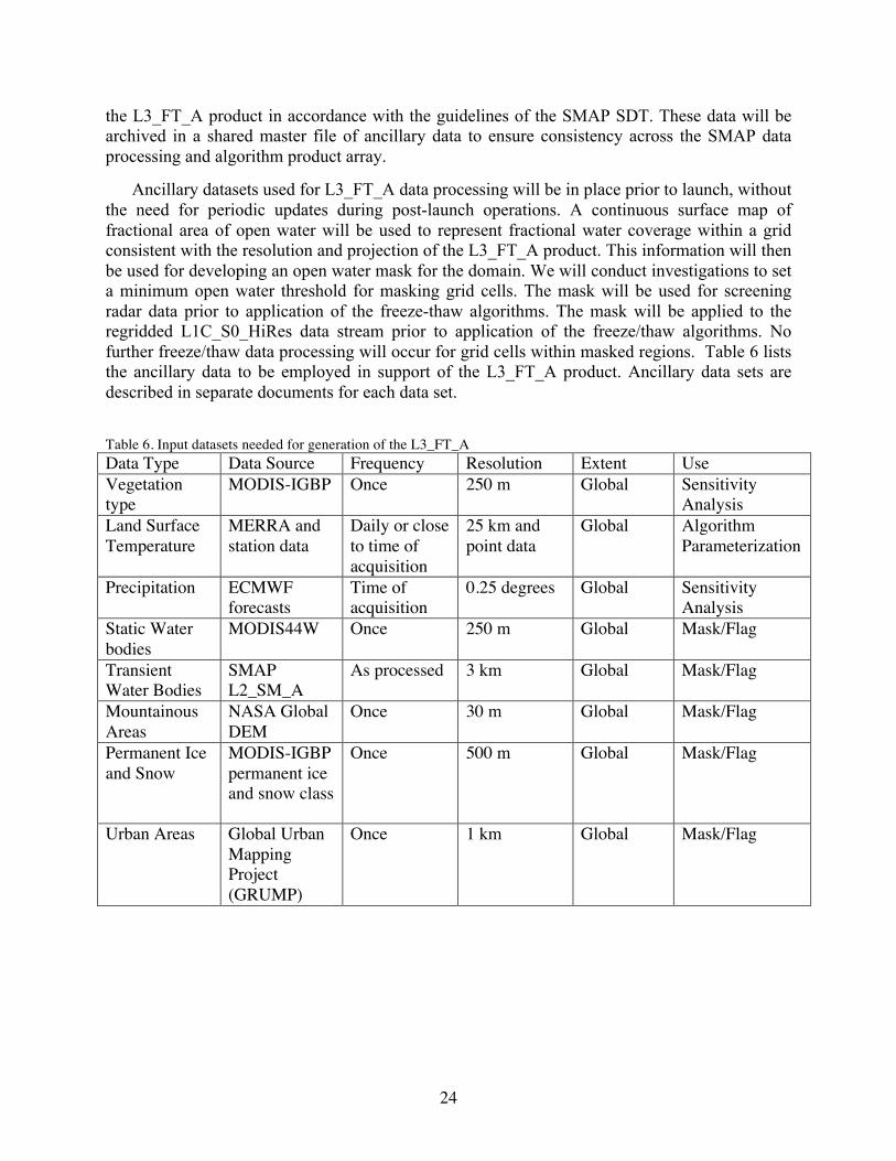
Ancillary datasets used for L3_FT_A data processing will be in place prior to launch, without the need for periodic updates during post-launch operations. A continuous surface map of fractional area of open water will be used to represent fractional water coverage within a grid consistent with the resolution and projection of the L3_FT_A product. This information will then be used for developing an open water mask for the domain. We will conduct investigations to set a minimum open water threshold for masking grid cells. The mask will be used for screening radar data prior to application of the freeze-thaw algorithms. The mask will be applied to the regridded L1C_S0_HiRes data stream prior to application of the freeze/thaw algorithms. No further freeze/thaw data processing will occur for grid cells within masked regions. Table 6 lists the ancillary data to be employed in support of the L3_FT_A product. Ancillary data sets are described in separate documents for each data set. Table 6. Input datasets needed for generation of the L3_FT_A Data Type Data Source Frequency Resolution Extent Use Vegetation type

MODIS-IGBP Once 250 m Global Sensitivity Analysis

Land Surface Temperature

MERRA and station data

Daily or close to time of acquisition

25 km and point data

Global Algorithm Parameterization

Precipitation ECMWF forecasts

Time of acquisition

0.25 degrees Global Sensitivity Analysis

Static Water bodies

MODIS44W Once 250 m Global Mask/Flag

Transient Water Bodies

SMAP L2_SM_A

As processed 3 km Global Mask/Flag

Mountainous Areas

NASA Global DEM

Once 30 m Global Mask/Flag

Permanent Ice and Snow

MODIS-IGBP permanent ice and snow class

Once 500 m Global Mask/Flag

Urban Areas Global Urban Mapping Project (GRUMP)

Once 1 km Global Mask/Flag

25

4.2.3 CALIBRATION AND VALIDATION Freeze/thaw algorithm performance will be assessed using the SMAP SDS Algorithm

Testbed and available L-band microwave remote sensing datasets within the SMAP freeze/thaw domain, including satellite based observations from PALSAR and SMOS, and relatively fine scale remote sensing and biophysical data from in situ towers and airborne field campaigns, e.g. PALS and CARVE experiment (Jackson et al., 2011).

The algorithm results will be evaluated across regional gradients in climate, land cover, terrain and vegetation biomass through direct comparisons to existing surface biophysical measurement network observations including air/soil/vegetation temperature, snow depth and snow water equivalent and eddy covariance CO2 exchange. The relationship between the algorithm freeze/thaw state and the in situ sampling data will be established. Major focus areas include relations between the local/solar timing of satellite AM and PM overpasses and diurnal variability in local surface temperature and freeze/thaw state dynamics; the spatial and temporal distribution and stability of L-band radar backscatter under frozen and non-frozen conditions, and the effects of sub-grid scale land cover and topographic heterogeneity on the aggregate freeze/thaw signal within the sensor footprint.

Biophysical measurements from in situ station measurement networks will be used to drive physical models within the SMAP Algorithm Testbed for spatial and temporal extrapolation of land surface dielectric and radar backscatter properties and associated landscape freeze/thaw dynamics. These results will be compared with field campaign measurements and satellite based retrievals of these properties. Model sensitivity studies will be conducted to assess L3_FT algorithm and freeze/thaw classification uncertainties in response to uncertainties in sensor sigma-0 error and terrain and land cover heterogeneity within the sensor FOV.

4.2.4 TEST PROCEDURES Accuracy requirements for the L3 freeze/thaw product state that the freeze/thaw status of the

aggregate vegetation-soil layer shall be determined sufficiently to characterize the low-temperature constraint on vegetation net primary productivity, and surface-atmosphere CO2 exchange (see Section 1). In order to achieve these requirements, the L3_FT_A product will meet or exceed a 2 day temporal repeat and 3 km spatial resolution, sufficient to resolve annual variations in net primary productivity and growing season length to within 3% (i.e., 0.05 tons C ha-1 over a ~100-day growing season) accuracy over a minimum mission length of two complete seasonal cycles. Validated science data products shall be made available to the science community starting no later than 12 months after completion of the initial on-orbit checkout period. Selected data products that have not undergone full validation will be made available in near real-time for time-critical applications including processing of the SMAP L3_SM_P data stream, operational forecast demonstrations and hydrometeorologic and carbon cycle monitoring.

Procedures for testing and documenting the performance of L3_FT_A algorithms in accordance with SMAP accuracy guidelines will primarily involve application and testing of the algorithms over the freeze/thaw domain using multi-scale satellite microwave remote sensing time-series data including JERS-1, ALOS PALSAR, SeaWinds, SSM/I and SMOS. The algorithms will be evaluated through direct comparisons to existing surface biophysical

26

measurement network observations, including air/soil/vegetation temperature, snow depth and snow water-equivalent, eddy covariance CO2 exchange, and seasonal anomalies of atmospheric CO2 concentrations. Algorithm results have also been compared with MODIS/AVHRR optical-IR satellite remote sensing observations of gross and net primary production (GPP and NPP), canopy phenology and leaf area index anomalies, and more detailed ecosystem process model simulations (Biome-BGC and TEM) of the landscape thermal regime and carbon cycle dynamics (e.g., Kimball et al., 2001; 2004a,b; McDonald et al., 2004).

We plan to apply L3_FT_A algorithms and evaluate model performance using aircraft, satellite, surface measurement network and modeling data from focused simulation studies conducted across regional boreal environmental (e.g., vegetation, thermal, land cover, topographic) gradients. We will also assemble a prototype data stream for the SMAP freeze/thaw domain with similar L-band, 3km spatial scale and 2-day temporal repeat characteristics as SMAP for intensive testing of freeze/thaw algorithm performance. This data stream will be developed for intensive study sites (e.g., Ameriflux and ALECTRA sites) and the North American component of the SMAP freeze/thaw acquisition domain using existing JERS-1 (1992-1998) and PALSAR (2006-2011) L-band time-series data and radar backscatter simulation models (e.g., MIMICS). These activities will be coordinated and conducted with members of the SMAP SDT. We will conduct comparison studies between SMAP L3_FT_A algorithm results and process model simulations of freeze-thaw fields and ecosystem processes driven by surface weather station networks. We will also conduct forward modeling of radar backscatter (e.g., MIMICS) dynamics and validate model results using JERS-1 and PALSAR time series data. We will continue to evaluate SMAP spatial accuracy requirements through resolution degradation exercises using the prototype JERS-1 and PALSAR based L-band σo data stream. We will also continue to evaluate SMAP temporal resolution requirements and sensor overpass acquisition trade-offs through spatial and temporal scale degradation studies. We will employ available terrain, land cover maps to evaluate land cover, terrain and open water effects on L3_FT_A algorithms and the potential for enhanced algorithms and products.

4.2.5 ALGORITHM BASELINE SELECTION

The current baseline algorithm is the algorithm of choice as it is best suited to fulfill mission requirements. Although aspects of the optional algorithms may be examined as part on on-going research, no changes are anticipated to the baseline algorithm prior to launch and operations.

5 CONSTRAINTS, LIMITATIONS, AND ASSUMPTIONS

Constraints and limitations of the algorithm will be assessed using the test procedures discussed in Section 4.1.3 above. Caveats will be identified appropriately.

27

6 REFERENCES

Armstrong, R.L. and Brodzik, M.J. (1995). An Earth-gridded SSM/I data set for cryospheric studies and global change monitoring. Advances in Space Research, 16(10), 155-163.

Betts, A. K., Viterbo, P., Beljaars, A. C. M., van den Hurk, B. J. J. M. (2000). Impact of BOREAS on the ECMWF forecast model, Journal of Geophysical Research, 106(D24) 33,593-33,604.

Black, T. A., Chen, W. J., Barr, A. G., Arain, M. A., Chen, Z., Nesic, Z., Hogg, E. H., Neumann, H. H., and Yang, P. C. (2000). Increased carbon sequestration by a boreal deciduous forest in years with a warm spring. Geophys. Res. Lett. 27(9), 1271-1274.

Canny, J. F. (1986). “A Computational Approach to Edge Detection.” IEEE Trans. Pattern Analysis and Machine Intelligence, 8 (6): 679-698.

Churkina, G., and S.W. Running, 1998. Contrasting climatic controls on the estimated productivity of different biomes. Ecosystems 1, 206-215.

Entekhabi, D., E. Njoku, P. Houser, M. Spencer, T. Doiron, J. Smith, R. Girard, S. Belair, W. Crow, T. Jackson, Y. Kerr, J. Kimball, R. Koster, K. McDonald, P. O’Neill, T. Pultz, S. Running, J.C. Shi, E. Wood, and J. Van Zyl, 2004. The Hydrosphere State (HYDROS) mission concept: An Earth System Pathfinder for global mapping of soil moisture and land freeze/thaw. Transactions in Geoscience and Remote Sensing 42, 10, 2184-2195.

Entekhabi, D., E. Njoku, P. O’Neill, K. Kellogg, W. Crow, W. Edelstein, J. Entin, S. Goodman, T. Jackson, J. Johnson, J. Kimball, J. Piepmeier, R. Koster, K. McDonald, M. Moghaddam, S. Moran, R. Reichle, J. C. Shi, M. Spencer, S. Thurman, L. Tsang, J. Van Zyl, “The Soil Moisture Active and Passive (SMAP) Mission”, Proceedings of the IEEE, 98(5), 2010.

Frolking S., K. McDonald, J. Kimball, R. Zimmermann, J.B. Way and S.W. Running, 1999. Using the space-borne NASA Scatterometer (NSCAT) to determine the frozen and thawed seasons of a boreal landscape. Journal of Geophysical Research 104(D22), 27,895-27,907.

Gamon, J.A., K.F. Huemmrich, J. Chen, D. Fuentes, F.G. Hall, J.S. Kimball, S. Goetz, J. Gu, K.C. McDonald, J.R. Miller, M. Moghaddam, D.R. Peddle, A.F. Rahman, J.-L. Roujean, E.A. Smith, C.L. Walthall, and P. Zarco-Tejada, 2004. Remote sensing in BOREAS: Lessons learned. Remote Sensing of Environment 89(2), 139-162.

Goulden, M.L., Wofsy, S.C., Harden, J.W., Trumbore, S.E., Crill, P.M., Gower, S.T., Fries, T., Daube, B.C., Fan, S.-M., Sutton, D.J., Bazzaz, A., and Munger, J.W. (1998). Sensitivity of boreal forest carbon balance to soil thaw. Science 279(9), 214-217.

Jackson, T., J. Kimball, R. Reichle, W. Crow, A. Colliander, E. Njoku, 2011. Soil Moisture Active and Passive (SMAP) Mission Science Calibration and Validation Plan, SMAP Science Document. No: 014, Version: 1.2 (Preliminary Release)

Jarvis, P., and Linder, S. (2000). Constraints to growth of boreal forests. Nature, 405, 904-905.

Kim, Y., J.S. Kimball, K.C. McDonald and J. Glassy, 2010. Developing a global data record of daily landscape freeze/thaw status using satellite passive microwave remote sensing. IEEE Transactions on Geoscience and Remote Sensing 49, 949-960.

28

Kimball, J., McDonald, K. C., Keyser, A. R., Frolking, S., and Running, S. W. (2001). Application of the NASA Scatterometer (NSCAT) for Classifying the Daily Frozen and Non-Frozen Landscape of Alaska, Remote Sensing of Environment, 75, 113-126.

Kimball, J.S., K.C. McDonald, S. Frolking and S.W. Running. 2004. Radar remote sensing of the spring thaw transition across a boreal landscape. Remote Sensing of Environment 89(2), 163-175.

Kimball, J.S., K.C. McDonald, S.W. Running, and S. Frolking, 2004a. Satellite radar remote sensing of seasonal growing seasons for boreal and subalpine evergreen forests. Remote Sensing of Environment 90, 243-258.

Kimball, J.S., M. Zhao, K.C. McDonald, F.A. Heinsch, and S. Running, 2004b. Satellite observations of annual variability in terrestrial carbon cycles and seasonal growing seasons at high northern latitudes. In Microwave Remote Sensing of the Atmosphere and Environment IV, G. Skofronick Jackson and S. Uratsuka (Eds.), Proceedings of SPIE – The International Society for Optical Engineering, 5654, 244-254.

Kraszewski, A. (editor). (1996), Microwave Aquametry: Electromagnetic Wave Interaction with Water-Containing Materials, IEEE Press, Piscataway, N.J., 484 pp.

Kuga, Y., Whitt, M. W., McDonald, K. C. and Ulaby, F. T., 1990. Scattering Models for Distributed Targets. In Radar Polarimetry for Geoscience Applications, Ulaby F. T. and Elachi C.,(Ed.), Artech House: Dedham, MA.

McDonald, K.C, and J.S. Kimball , 2005. Hydrological application of remote sensing: Freeze-thaw states using both active and passive microwave sensors. Encyclopedia of Hydrological Sciences. Vol. 5., M.G. Anderson and J.J. McDonnell (Eds.), John Wiley & Sons Ltd.

McDonald, K.C., J.S. Kimball, E. Njoku, R. Zimmermann, and M. Zhao, 2004a. Variability in springtime thaw in the terrestrial high latitudes: Monitoring a major control on the biospheric assimilation of atmospheric CO2 with spaceborne microwave remote sensing. Earth Interactions 8(20), 1-23.

McDonald, K.C., J.S. Kimball, M. Zhao, E. Njoku, R. Zimmermann, and S.W. Running, 2004b. Spaceborne microwave remote sensing of seasonal freeze-thaw processes in the terrestrial high latitudes: Relationships with land-atmosphere CO2 exchange. In Microwave Remote Sensing of the Atmosphere and Environment IV, G. Skofronick Jackson and S. Uratsuka (Eds.), Proceedings of SPIE – The International Society for Optical Engineering, 5654, 167-178.

National Research Council, “Earth Science and Applications from Space: National Imperatives for the Next Decade and Beyond,” pp. 400, 2007.

Nemani, R.R., Keeling C. D., Hashimoto H., Jolly W.M., Piper S.C., Tucker C.J., Myneni R.B., and Running S.W. (2003). Climate-driven increases in global terrestrial net primary production from 1982 to 1999. Science 300, 1560-1563.

Podest, E. (2006), "Monitoring Boreal Landscape Freeze/Thaw Transitions with Spaceborne Microwave Remote Sensing". Ph.D. dissertation, University of Dundee.

Raney, K. R. (1998), Radar fundamentals: Technical perspective, In Principles and Applications of Imaging Radar, Vol. 2, F. M. Henderson and A. J. Lewis (Eds.), John Wiley and Sons Inc., New York, pp. 9-130.

29

Rawlins, M.A, K.C. McDonald, S. Frolking, R.B. Lammers, M. Fahnestock, J.S. Kimball, C.J. Vorosmarty, 2005: Remote Sensing of Pan-Arctic Snowpack Thaw Using the SeaWinds Scatterometer, Journal of Hydrology 312/1-4 pp. 294-311

Rignot E., and Way, J.B. (1994). Monitoring freeze-thaw cycles along north-south Alaskan transects using ERS-1 SAR, Remote Sensing of Environment, 49, 131-137.

Rignot, E., Way, J.B., McDonald, K., Viereck, L., Williams, C., Adams, P., Payne, C., Wood, W., and Shi, J. (1994). Monitoring of environmental conditions in taiga forests using ERS-1 SAR, Remote Sensing of Environment, 49, 145-154.

Ulaby, F. T., Moore, R. K. and Fung, A. K. (1986), Microwave Remote Sensing: Active and Passive, Vol. 1-3, Artec House:Dedham MA

Ulaby, F. T., Sarabandi, K., McDonald, K., Whitt, M. and Dobson, M. C. (1990). Michigan Microwave Canopy Scattering Model (MIMICS), International Journal of Remote Sensing, 11(7), 1223-1253.

Vaganov, E.A., Hughes, M.K., Kirdyanov, A.V., Schweingruber, F.H., and Silkin, P.P. (1999). Influence of snowfall and melt timing on tree growth in subarctic Eurasia. Nature 400, 149-151.

Way, J. B., Paris, J., Kasischke, E., Slaughter, C., Viereck, L., Christensen, N., Dobson, M. C., Ulaby, F. T., Richards, J., Milne, A., Sieber, A., Ahern, F. J., Simonett, D., Hoffer, R., Imhoff, M. and Weber, J. (1990). The effect of changing environmental conditions on microwave signatures of forest ecosystems: preliminary results of the March 1988 Alaskan aircraft SAR experiment. Int. J. Remote Sensing, 11, 1119-1144.

Way, J.B., Rignot, E., McDonald, K., Oren, R., Kwok, R., Bonan, G., Dobson, M. C., Viereck, L. and Roth, J.E. (1994). Evaluating the type and state of Alaska taiga forests with imaging radar for use in ecosystem flux models, IEEE Trans. Geosci. Rem. Sens., 32(2).

Way, J. B., Zimmermann, R., Rignot, E., McDonald, K. and Oren, R. (1997). Winter and Spring Thaw as Observed with Imaging Radar at BOREAS, Journal of Geophysical Research, 102(D24), 29673-29684.

Wegmuller, U. (1990), The effect of freezing and thawing on the microwave signatures of bare soil, Remote Sens. Environ. 33, 123-135.

Wismann, V. (2000). Monitoring of seasonal thawing in Siberia with ERS scatterometer data. IEEE Trans. Geosci. Rem. Sens., 38,1804–1809.

30

APPENDIX 1: GLOSSARY [Adapted from: Earth Observing System Data and Information System (EOSDIS) Glossary

http://www-v0ims.gsfc.nasa.gov/v0ims/DOCUMENTATION/GLOS-ACR/glossary.of.terms.html.]

ALGORITHM. (1) Software delivered by a science investigator to be used as the primary tool in the generation of science products. The term includes executable code, source code, job control scripts, as well as documentation. (2) A prescription for the calculation of a quantity; used to derive geophysical properties from observations and to facilitate calculation of state variables in models.

ANCILLARY DATA. Data other than instrument data required to perform an instrument's data processing. They include orbit data, attitude data, time information, spacecraft engineering data, calibration data, data quality information, data from other instruments (spaceborne, airborne, ground-based) and models.

BROWSE. A representation of a data set or data granule used to pre-screen data as an aid to selection prior to ordering. A data set, typically of limited size and resolution, created to rapidly provide an understanding of the type and quality of available full resolution data sets. It may also enable the selection of intervals for further processing or analysis of physical events. For example, a browse image might be a reduced resolution version of a single channel from a multi-channel instrument. Note: Full resolution data sets may be browsed.

BROWSE DATA PRODUCT. Subsets of a larger data set, generated for the purpose of allowing rapid interrogation (i.e., browse ) of the larger data set by a potential user. For example, the browse product for an image data set with multiple spectral bands and moderate spatial resolution might be an image in two spectral channels, at a degraded spatial resolution. The form of browse data is generally unique for each type of data set and depends on the nature of the data and the criteria used for data selection within the relevant scientific disciplines.

Dynamic Browse. Refers to the generation of a browse product, including subsetting and/or resampling of data, by command of the user engaged in the browse activity. The browse data set is built in real-time, or near-real-time, as part of the browse activity.

Static Browse. Refers to interrogation of browse products which have been generated (through subsetting and/or resampling) before any user browses that particular data set.

CALIBRATION. (1) The activities involved in adjusting an instrument to be intrinsically accurate, either before or after launch (i.e., “instrument calibration”). (2) The process of collecting instrument characterization information (scale, offset, nonlinearity, operational, and environmental effects), using either laboratory standards, field standards, or modeling, which is used to interpret instrument measurements (i.e., “data calibration”).

CALIBRATION DATA. The collection of data required to perform calibration of the instrument science and engineering data, and the spacecraft or platform engineering data. It includes pre-flight calibrator measurements, calibration equation coefficients derived from calibration software routines, and ground truth data that are to be used in the data calibration processing routine.

CORRELATIVE DATA. Scientific data from other sources used in the interpretation or validation of instrument data products, e.g. ground truth data and/or data products of other instruments. These data are not utilized for processing instrument data.

31

DATA PRODUCT. A collection (1 or more) of parameters packaged with associated ancillary and labeling data. Uniformly processed and formatted. Typically uniform temporal and spatial resolution. (Often the collection of data distributed by a data center or subsetted by a data center for distribution.) There are two types of data products:

Standard - A data product produced by a community consensus algorithm. Typically produced for a wide community. May be produced routinely or on-demand. If produced routinely, typically produced over most or all of the available independent variable space. If produced on-demand, produced only on request from users for particular research needs typically over a limited range of independent variable space.

Special - A data product produced by a research status algorithm. May migrate to a community consensus algorithm at a later time. If adequate community interest exists, the product may be archived and distributed by a DAAC.

DATA PRODUCT LEVEL. Data levels 1 through 4 as designated in the EOSDIS Product Type and Processing Level Definitions document.

Raw Data - Data in their original packets, as received from the observer, unprocessed.

Level 0 - Raw instrument data at original resolution, time ordered, with duplicate packets removed.

Level 1A - Reconstructed unprocessed instrument data at full resolution, time referenced, and annotated with ancillary information, including radiometric and geometric calibration coefficients and georeferencing parameters (i.e., platform ephemeris) computed and appended, but not applied to Level 0 data.

Level 1B - Radiometrically corrected and geolocated Level 1A data that have been processed to sensor units.

Level 1C - Level 1B data that have been spatially resampled.

Level 2 - Derived geophysical parameters at the same resolution and location as the Level 1 (1B or 1C) data.

Level 3 - Geophysical or sensor parameters that have been spatially and/or temporally re-sampled (i.e., derived from Level 2 or Level 1 data).

Level 4 - Model output and/or results of lower level data that are not directly derived by the instruments.

DISTRIBUTED ACTIVE ARCHIVE CENTER (DAAC). An EOSDIS facility that archives, and distributes data products, and related information. An EOSDIS DAAC is managed by an institution such as a NASA field center or a university, under terms of an agreement with NASA. Each DAAC contains functional elements for archiving and disseminating data, and for user services and information management. Other (non-NASA) agencies may share management and funding responsibilities for the active archives under terms of agreements negotiated with NASA.

GRANULE. The smallest aggregation of data which is independently managed (i.e., described, inventoried, retrievable). Granules may be managed as logical granules and/or physical granules.

32

GUIDE. A detailed description of a number of data sets and related entities, containing information suitable for making a determination of the nature of each data set and its potential usefulness for a specific application.

INSTRUMENT DATA. Data specifically associated with the instrument, either because they were generated by the instrument or included in data packets identified with that instrument. These data consist of instrument science and engineering data, and possible ancillary data.

Instrument Engineering Data. Data produced by the engineering sensor(s) of an instrument that is used to determine the physical state of an instrument in order to operate it, monitor its health, or aid in processing its science data.

Instrument Science Data. Data produced by the science sensor(s) containing the primary observables of an instrument, usually constituting the mission of that instrument.

METADATA. (1) Information about a data set which is provided by the data supplier or the generating algorithm and which provides a description of the content, format, and utility of the data set. Metadata provide criteria which may be used to select data for a particular scientific investigation. (2) Information describing a data set, including data user guide, descriptions of the data set in directories, and inventories, and any additional information required to define the relationships among these.

NEAR REAL-TIME DATA. Data from the source that are available for use within a time that is short in comparison to important time scales in the phenomena being studied.

ORBIT DATA. Data that represent spacecraft locations. Orbit (or ephemeris) data include: Geodetic latitude, longitude and height above an adopted reference ellipsoid (or distance from the center of mass of the Earth); a corresponding statement about the accuracy of the position and the corresponding time of the position (including the time system); some accuracy requirements may be hundreds of meters while other may be a few centimeters.

PARAMETER. A measurable or derived variable represented by the data (e.g. air temperature, snow depth, relative humidity.

QUICK-LOOK DATA. Data available for examination within a short time of receipt, where completeness of processing is sacrificed to achieve rapid availability.

RAW DATA. Numerical values representing the direct observations output by a measuring instrument transmitted as a bit stream in the order they were obtained. (Also see DATA PRODUCT LEVEL.)

REAL-TIME DATA. Data that are acquired and transmitted immediately to the ground (as opposed to playback data). Delay is limited to the actual time (propagation delays) required to transmit the data.

SPACECRAFT ENGINEERING DATA. Data produced by the engineering sensor(s) of a spacecraft that are used to determine the physical state of the spacecraft, in order to operate it or monitor its health.