smart grid model - wordpress.com€¦ · smart grid model 1 october 2014 ieee/acm toulouse....

Guillaume Guérard

UVSQ

A context-free autonomous

SMART GRID MODEL

1

October 2014IEEE/ACMToulouse

Optimization in a complex system:

How to optimize the consumption, the production and the distribution of the energy in a Smart Grid.

Multicriteria optimization:

-Resilience.-Reliability.-Minimal cost (flow, production, consumption).-Supply and demand management.

Problematic

2

The actual Energy Grid is based on Nikola Tesla works (1888).

Shortcoming:- Structure: integration of Renewable

Energy, management of batteries, NTIC.

- Consumption: congestion, network latency, profitability of plants.

Smart Grid : network integrating behaviors and actions of users.

Industrial goals

3

Global behavior:

- To smooth the curve

- To optimize supply and demand

- To guarantee QoS.

New network characteristics

4

• Self-Healing

• Flexibility

• Predictive

• Interactive

• Optimal

• Sure.

Actual models

5

Most of simulations/models are done

on a specific case with a limited

evolution.

Disadvantage of Cartesian approach:

- Computational time depending of

the size of the instance.

- Data storage, data mining.

- Models are not « plug-and-play »

and « friendly ».

Objective: to optimize in real time a context-free Smart Grid.

A complex system

• It is difficult to find an objective function solving the overall problem.

• The number of variables involved range up to thousands of entities.

Kirkpatrick et al. (1983)

• To find an apppropriateclass of algorithms for optimizing local applications.

• Parameters between each applications should be granted.

Grefenstette (1986)

6

Goal: to find a method in order to analyse and define a model of a complex system.

Smart Grid

Complex system approach Algorithms Smart system

7

Complex system approach

8

Bottom-up analysis

9

Global equilibrium

Feedback

Global objectives

Algorithms

Optimization

• Interaction

• Communication

• Behaviors

Subsystem

Structure Agent Goal

Would it not be better and permissive to understand the fundamentals and drivers of Smart Grid rather than imposing new and often incompatible technologies?

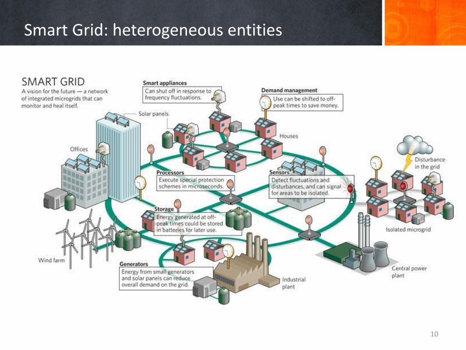
Smart Grid: heterogeneous entities

10

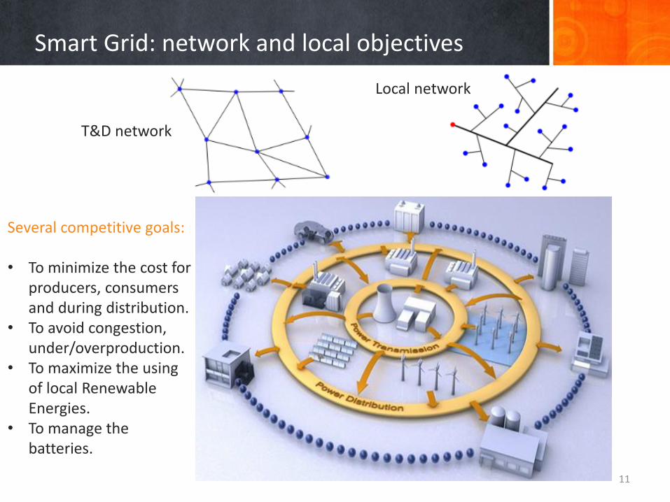
Smart Grid: network and local objectives

11

T&D network

Local network

Several competitive goals:

• To minimize the cost for producers, consumers and during distribution.

• To avoid congestion, under/overproduction.

• To maximize the using of local Renewable Energies.

• To manage the batteries.

Device’s data for a smart management

12

Device Power, in Watts Consumption scheme Usage time Average consumption

Converted data for the model:

• Devices (Consumer or Producer).• Consumption: Power, in Watts.• Priority: it depends on several data of the device and

its impact on demand-side management.• Cost: used by each device in all algorithms.

Industrial data

Optimization of a context-free Smart Grid

13

General process

14

• Bottom-up– First allocation following

prognostics

– If prognostics are true, the iteration is ended.

• Top-down– Equilibrium between supplies

and demands

– Final allocation and stats for future iterations.

Bottom - up

Top - down

Local level

15

Update

• Data update (devices, sensors, batteries).

First allocation

• To compare prognostics to data.

First allocation II

• Result of local knapsack problem.

Iteration: each 5min.

Microgrid level

16

Game theory

• Demand-side management

• Feedback with T&D

• Prognostics are calculated (infinite values).

Final allocation

• Local knapsack problem

• Knapsack bottom-up resolution.

Strategies

17

Strategies Priority Cost

Simple device using Standard Standard

Peak shaving Increasing Decreasing

Conservation Increasing Decreasing

Load shifting Increasing/Decreasing ‘’

Congestion Increasing Standard

Under-consumption Decreasing Standard

Over-consumption Standard Increasing

- Priority: impact of feedback on the priority of the devices- Cost: impact of feedback on the cost of the strategy.

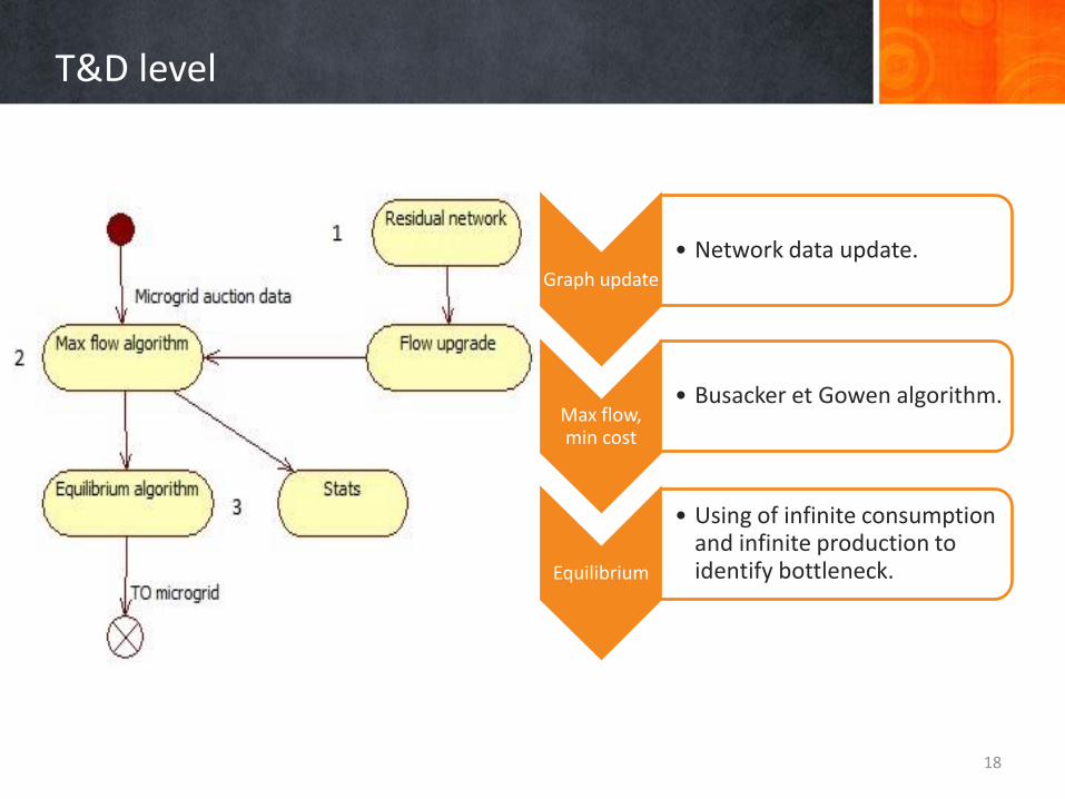
T&D level

18

Graph update

• Network data update.

Max flow, min cost

• Busacker et Gowen algorithm.

Equilibrium

• Using of infinite consumption and infinite production to identify bottleneck.

T&D network

19

• Idea • Network

How to build a dynamic graph ?

Benefits: real time management, detailed network, easy to parametrize.

Adhesion function and interior function for a given criterion.

To define lower and upper cost.

To prevent congestion.

Resolved by Busacker and Gowenalgorithms.

Smart Grid: an iteration.

20

- Local first allocation;- Game between microgrids and producers;- Feedback (by infinite values);- Equilibrium: local to microgrid allocation by

knapsack problem resolution.

Smart system

21

How to smooth the curve ?

22

• Slope and regularity • K-Lipschitz function

Local algorithm cannot see the overall results.

General knapsack problem

• Knapsack problem under constraints:

– our tout instant T

– max 𝑖=1𝑛 𝑥𝑖 𝑢𝑖

• xi=1 si la demande en énergie est satisfaite à l’instant T, 0 sinon.

• Ui= valeur calculée lors du sac-à-dos ou lors des enchères (modèle économique).

23

– For each iteration

max

𝑖=1

𝑛

𝑥𝑖 𝑢𝑖

s.t. 𝑖=1𝑛 𝑥𝑖𝑤𝑖 ≤ 𝑊

𝑗

𝑖=1𝑛 𝑎𝑖

𝑘 𝑤𝑖 ≤ 𝑊𝑘

𝑖=1𝑚 𝑎𝑖

𝑘 = 𝑥𝑖

𝑗=1𝑎𝑙𝑙(𝑗)𝑊𝑗 = 𝑘=1

all(𝑘)𝑊𝑘

• j for each microgrid

• k for each flow• Wj consumption of each

microgrid.

How to increase the efficiency of algorithms ?

How to enhance the system ?

• Convex maximization:– Knapsack problem is a

quadratic convex maximization problem.

– Two quick and simple algorithms to resolve this problem (<5min for 300 entities).

• Enhance the model:– To compare result of the KP

with the iteration with same data.

– Some parameters impact the effect of each strategy costs.

24

Local benefits

• Benefits:– Using of local renewable

energy.

– Battery/electric vehicles management with some plugin.

– Minimal using of the general distribution network.

– Gross and net consumption.

25

Global benefits

• For the producer:– The curve is smoothed– No more peaks– Reduction of carbon

uses.

• For the consumers:– Demand-side

management reduce global cost.

– Reduced cost in function of participation.

26

Publications

27

Journal

Guérard, G., Amor, S. B., & Bui, A. (2012). Survey on smart grid modelling. International Journal of Systems, Control and

Communications, 4(4), 262-279.

Ahat, M., Amor, S. B., Bui, M., Bui, A., Guérard, G., & Petermann, C. (2013). Smart grid and optimization. American Journal of

Operations Research, 3, 196.

Guérard, G., & Tseveendorj, I. (2014), Inscribed Ball and Enclosing Box for Convex Maximization Problems. Optimization Letters (2nd

revised edition).

Conferences

Guérard, G., Amor, S. B., & Bui, A. (2012, April). Approche système complexe pour la modélisation des smart grids. In 13th Roadef

Conference, Angers, France (pp. 263-264).

Guérard, G., Amor, S. B., & Bui, A. (2012). A Complex System Approach for Smart Grid Analysis and Modeling. In KES (pp. 788-797).

Amor, S. B., Bui, A., & Guérard, G. (2013). Méthode d’Analyse d’un Système Complexe pour la Recherche Opérationnelle: Smart Grid.

Recherche Opérationnelle et Aide à la DEcision Française (ROADEF’13).

MAGO14, Guérard, G., & Tseveendorj, I. (2014) Largest Inscribed Ball and Minimal Enclosing Box for Convex Maximization Problems.

IEEE/ACM'14, Guérard, G., Amor, S. B., & Bui, A. (2014). A Context-Free Smart Grid Model Using Complex System Approach.

ProjectEPIT 2.0 (Bouygues, Alstom; Renault, Supélec, Eurodecision) 2011-2014

GARE (SNCF) 2011-2012

•

Quel message voulez-vous diffuser ?

Smart Grid

28

Ancienne itération

• Exemple :– 2 centrales– 2 microgrids– 5 maisons

• Résultats / pronostiques :– Maison1 : 4/4– Maison2 : 5/7– Maison3 : 17/12– Maison4 : 4/9– Maison5 : 10/6– Centrale1 : 20/20– Centrale2 : 21/20

29

Mise à jour des consommations

Maison1 Maison2 Maison3 Maison4 Maison5

1/0/811/1/803/0/835/2/7520/4/20

Prévision : 4Conso_moy : 5

1/0/161/0/162/1/153/0/184/3/75/3/5

Prévision: 6Conso_moy: 7

1/01/010/0

Prévision: 12

1/0/331/1/323/0/353/2/294/1/328/4/8

Prévision: 8Conso_moy: 9

1/03/0

Prévision: 6

30

Calcul de la valeur d’un appareil i dans une maison : valeuri=(poidsmax*prioritémax)-(poidsi*prioritéi) + poidsi

Consommation résiduelle : le niveau local ne demande que ce qu’il ne produit pas lui-même (de même pour le microgrid).

-> Demande nette de consommationDSM : seul les appareils intelligents/domotique peuvent avoir une priorité supérieur à 0.

Type de jeux : utilité maximale

31

Stratégie local : somme des utilités*consommation/priorité (>1)Stratégie T&D : somme des (utilité/priorité-v)*consommationv (valeur unitaire) : moyenne de l’utilité par unité de consommation

Stratégie(Utilité)

Maison 1 v=34

Maison 2V=10

Maison 3 Maison 4V=22,5

Maison 5

0 330/194 77/27 Done 138/47 Done

1 410/240 107/37 298/56,5

2 620/257,5 341,5/32,5

3 none 125/-36

4 720/-322,5 357,5/-131,5

5 none

Enchère (consommation)

10 7 12 12 4

Mise-à-jour du routage

• Mise-à-jour– Centrale2 : production de 21 à 20

– Microgrid2 : consommation de 31 à 25

32

Graphe résiduel et nouveau routage

1. Mise-à-jour du réseau :• Production• Mise en place du graphe résiduel

2. Mise-à-jour du routage.3. Flot max par Ford-Fulkerson.

Nouveau routage et rétroaction

33

Résolution par Ford-fulkerson

1. Nous récompensons les deux Microgrids.2. Surproduction sur les deux centrales.

4. Détection des goulots d’étranglement(production et consommation) et de lacongestion.

Enchères finales

34

• Microgrid1– Maison1 : enchère de 4. – Maison2 : enchère de 8.

– Total : 12,– Prévision : 10,– Reçu i-1 : 9.

• Microgrid2– Maison3 : enchère de 13.– Maison4 : enchère de 11.– Maison5 : enchère de 4.

– Total : 28, – Prévision : 26, – Reçu i-1 : 31.

Consommation finale

Maison1 Maison2 Maison3 Maison4 Maison5

1/0/811/1/803/0/835/2/7520/4/20

Reçu : 4Consommé : 4Reste : 0

1/0/161/0/162/1/153/0/184/3/75/3/5


1/01/010/0


1/0/331/1/323/0/353/2/294/1/328/4/8


1/03/0


35

Poids/Priorité/Valeur, le résultat du KP local est en rouge, et du KP microgrid en vert.Il est possible de faire un jeu final pour la distribution des ressources.

Microgrid1 reste : 1Consommé : 1Reste : 0

Microgrid2 reste : 3Consommé : 3Reste : 0

Résultats de l’itération

• Exemple :– 2 centrales– 2 microgrids– 5 maisons

• Résultats / pronostiques :– Maison1 : 4/4+– Maison2 : 7/7+– Maison3 : 12/12-– Maison4 : 12/12– Maison5 : 4/4+– Centrale1 : 20/20+– Centrale 2 : 20/20+

36

La simulation

Module réseau de transport

Module consommation et production

Module distribution de l’énergie

Module gestion des pannes

Module réseau de communication

Coralie Petermann - UVSQ 37

smart grid model - wordpress.com€¦ · smart grid model 1 october 2014 ieee/acm toulouse....

Documents