SMASH: STRUCTURED MATRIX APPROXIMATION BY SEPARATION AND

HIERARCHY ∗

DIFENG CAI, EDMOND CHOW, LUCAS ERLANDSON, YOUSEF SAAD AND YUANZHE XI

Abstract. This paper presents an efficient method to perform Structured Matrix Approximation by Separationand Hierarchy (SMASH), when the original dense matrix is associated with a kernel function. Given points ina domain, a tree structure is first constructed based on an adaptive partitioning of the computational domain tofacilitate subsequent approximation procedures. In contrast to existing schemes based on either analytic or purelyalgebraic approximations, SMASH takes advantage of both approaches and greatly improves the efficiency. Thealgorithm follows a bottom-up traversal of the tree and is able to perform the operations associated with each node onthe same level in parallel. A strong rank-revealing factorization is applied to the initial analytic approximation in theseparation regime so that a special structure is incorporated into the final nested bases. As a consequence, the storageis significantly reduced on one hand and a hierarchy of the original grid is constructed on the other hand. Due to thishierarchy, nested bases at upper levels can be computed in a similar way as the leaf level operations but on coarsergrids. The main advantages of SMASH include its simplicity of implementation, its flexibility to construct varioushierarchical rank structures and a low storage cost. Rigorous error analysis and complexity analysis are conducted toshow that this scheme is fast and stable. The efficiency and robustness of SMASH are demonstrated through varioustest problems arising from integral equations, structured matrices, etc.

Key words. hierarchical rank structure, nested basis, error analysis, integral equation, Cauchy-like matrix

1. Introduction. The invention of the Fast Multipole Method (FMM) [55, 30] opened a newchapter in scientific computing methodology by unraveling a set of effective techniques revolvingaround the powerful principle of divide-and-conquer. When sets of points are far apart from eachother, the physical equations that couple them can be approximately expressed by means of a lowrank matrix. Among the many variations to this elegant idea, a few schemes have been developedto gain further efficiency by building hierarchical bases in order to expand the various low-rankcouplings. The resulting hierarchical rank structured matrices [13, 16, 24, 34], culminated in H2

matrices[37, 34], provide efficient solution techniques for structured linear systems (Toeplitz, Hankel,etc.)[61, 63, 67], integral equations [13, 16, 3, 43, 44], partial differential equations [16, 17, 34, 65],matrix equations [16, 28, 29] and eigenvalue problems [7, 62]. Though these methods come undervarious representations, they all start with a block partition of the coefficient matrix and approximatecertain blocks with low-rank matrices. The refinements of these techniques embodied in the H2

[16, 34, 35] and HSS [24, 60, 66] matrix representations take advantage of the relationships betweendifferent (numerically) low-rank blocks and use nested bases [34] to minimize computational costsand storage requirements. What is often not emphasized in the literature, is that this additionalefficiency in the solution phase is achieved at a rather high cost in the construction phase.

Both HSS andH2 matrices employ just two key ingredients: low-rank approximations and nestedbases. The low-rank approximation, or compression, methods exploited in these techniques can beclassified into three categories. The first category involves methods that rely on algebraic compres-sion, such as the SVD and the rank–revealing QR (RRQR) [33] which are among the most commonapproaches. Utilizing these techniques to compress low-rank blocks [11, 35, 66] will result in nestedbases that have orthogonal columns and an optimal rank. However, these methods will require thematrix entries to be explicitly available and usually lead to quadratic construction cost [35, 66].Other compression techniques, such as adaptive cross approximation (ACA) [3, 5, 6], extract alow-rank factorization based only on part of the matrix entries and this leads to a nearly linear con-struction cost. However, ACA may fail for general kernel functions and complex geometries due tothe heuristic nature of the method [15]. Other efficient low-rank approximation techniques include

∗The research of Edmond Chow was supported by NSF under grant ACI–1306573. The research of Yousef Saadand Yuanzhe Xi were both supported by NSF under grants DMS–1216366 and DMS–1521573 and by the MinnesotaSupercomputing Institute.

1

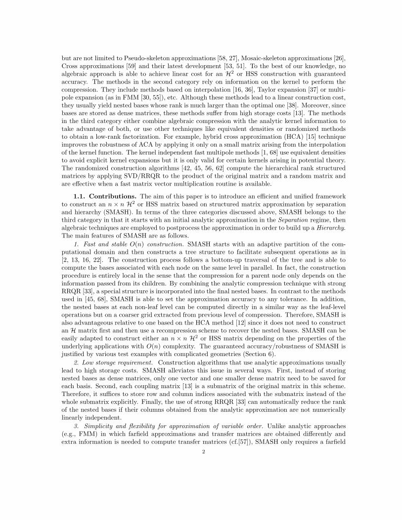
but are not limited to Pseudo-skeleton approximations [58, 27], Mosaic-skeleton approximations [26],Cross approximations [59] and their latest development [53, 51]. To the best of our knowledge, noalgebraic approach is able to achieve linear cost for an H2 or HSS construction with guaranteedaccuracy. The methods in the second category rely on information on the kernel to perform thecompression. They include methods based on interpolation [16, 36], Taylor expansion [37] or multi-pole expansion (as in FMM [30, 55]), etc. Although these methods lead to a linear construction cost,they usually yield nested bases whose rank is much larger than the optimal one [38]. Moreover, sincebases are stored as dense matrices, these methods suffer from high storage costs [13]. The methodsin the third category either combine algebraic compression with the analytic kernel information totake advantage of both, or use other techniques like equivalent densities or randomized methodsto obtain a low-rank factorization. For example, hybrid cross approximation (HCA) [15] techniqueimproves the robustness of ACA by applying it only on a small matrix arising from the interpolationof the kernel function. The kernel independent fast multipole methods [1, 68] use equivalent densitiesto avoid explicit kernel expansions but it is only valid for certain kernels arising in potential theory.The randomized construction algorithms [42, 45, 56, 62] compute the hierarchical rank structuredmatrices by applying SVD/RRQR to the product of the original matrix and a random matrix andare effective when a fast matrix vector multiplication routine is available.

1.1. Contributions. The aim of this paper is to introduce an efficient and unified frameworkto construct an n × n H2 or HSS matrix based on structured matrix approximation by separationand hierarchy (SMASH). In terms of the three categories discussed above, SMASH belongs to thethird category in that it starts with an initial analytic approximation in the Separation regime, thenalgebraic techniques are employed to postprocess the approximation in order to build up a Hierarchy.The main features of SMASH are as follows.

1. Fast and stable O(n) construction. SMASH starts with an adaptive partition of the com-putational domain and then constructs a tree structure to facilitate subsequent operations as in[2, 13, 16, 22]. The construction process follows a bottom-up traversal of the tree and is able tocompute the bases associated with each node on the same level in parallel. In fact, the constructionprocedure is entirely local in the sense that the compression for a parent node only depends on theinformation passed from its children. By combining the analytic compression technique with strongRRQR [33], a special structure is incorporated into the final nested bases. In contrast to the methodsused in [45, 68], SMASH is able to set the approximation accuracy to any tolerance. In addition,the nested bases at each non-leaf level can be computed directly in a similar way as the leaf-leveloperations but on a coarser grid extracted from previous level of compression. Therefore, SMASH isalso advantageous relative to one based on the HCA method [12] since it does not need to constructan H matrix first and then use a recompression scheme to recover the nested bases. SMASH can beeasily adapted to construct either an n × n H2 or HSS matrix depending on the properties of theunderlying applications with O(n) complexity. The guaranteed accuracy/robustness of SMASH isjustified by various test examples with complicated geometries (Section 6).

2. Low storage requirement. Construction algorithms that use analytic approximations usuallylead to high storage costs. SMASH alleviates this issue in several ways. First, instead of storingnested bases as dense matrices, only one vector and one smaller dense matrix need to be saved foreach basis. Second, each coupling matrix [13] is a submatrix of the original matrix in this scheme.Therefore, it suffices to store row and column indices associated with the submatrix instead of thewhole submatrix explicitly. Finally, the use of strong RRQR [33] can automatically reduce the rankof the nested bases if their columns obtained from the analytic approximation are not numericallylinearly independent.

3. Simplicity and flexibility for approximation of variable order. Unlike analytic approaches(e.g., FMM) in which farfield approximations and transfer matrices are obtained differently andextra information is needed to compute transfer matrices (cf.[57]), SMASH only requires a farfield

2

approximation, which can be readily obtained for almost all kernels, for example, via interpolation[36]. Moreover, the approximation rank in the compression on upper levels is independent of therank used in lower levels, which means that approximation rank can be chosen arbitrarily in thecompression at any level while still maintaining the H2 or HSS structure. This is due to the fact thatin each level of compression, SMASH produces transfer matrices directly, which is an advantage ofalgebraic approaches. For interpolation-based constructions, there are restrictions on the maximaldegree of basis polynomials in each level in order to maintain the H2 structure. [35].

1.2. Outline and Notation. The paper is organized as follows. In Section 2 we review low-rank approximations ([4, 13, 34]) associated with some kernel functions. Section 3 introduces SMASHfor the construction of hierarchical rank structured matrices with nested bases. The approximationerror and complexity of SMASH are analyzed in Section 4 and Section 5, respectively. Numericalexamples are provided in Section 6 and final concluding remarks are drawn in Section 7.

Throughout the paper, the following notation is used:• A: a dense matrix associated with a kernel function κ;• A: H2 or HSS approximation to A;• i = 1 : n denotes an enumeration of index i from 1 to n;• |·| denotes the cardinality of a finite set if the input is a set;• ‖·‖, ‖·‖F denote the L2 norm, Frobenius norm, respectively, and ‖A‖max denotes the ele-mentwise sup-norm of a matrix, i.e.,

‖A‖max := maxi,j

|ai,j |, A = [ai,j ]i,j ;

• diag(. . . ) denotes a block diagonal matrix;• Given a tree T , children(i) and lv(i) represent the children and level of node i, respectively,where root node is at level 1. The location of a node i at level l is denoted as li whenenumerated from left to right;

• Let X and Y be two nonempty finite sets of points and A be a matrix whose (i, j)th entry isdetermined by the ith point inX and jth point in Y . If i denotes the index set correspondingto a subset Xi of X , then A|i denotes the submatrix of A with rows determined by Xi.Furthermore, if index set j corresponds to a subset Yj of Y , then A|i×j denotes a submatrixof A whose rows and columns are determined by Xi and Yj, respectively.

2. Degenerate and low-rank approximations. Hierarchical rank structured matrices areoften used to approximate matrices after a block partition such that most blocks display certain(numerical) low-rank characteristics. For matrices derived from kernel functions, a low-rank ap-proximation can be determined when the kernel function can be locally approximated by degeneratefunctions [4]. In this section, we first review this property. For pedagogical reasons, we focus onthe kernel function 1/(x− y) but more general kernel functions can be handled in a similar way asdemonstrated in the numerical experiments section (Section 6).

2.1. Degenerate expansion. Consider the kernel function κ(x, y) on C× C defined by

(2.1) κ(x, y) =

1

x−y , if x 6= y,

dx, if x = y,

where the number dx ∈ C can be arbitrary. If x and y are far from each other (See Definition 2.1below), then κ(x, y) can be well approximated by a degenerate expansion

κ(x, y) ≈r−1∑

k=0

k∑

l=0

ck,lφk(x)ψl(y),

3

where φk and ψl are univariate functions. In fact, interpolation in the x variable yields the simplest,yet most general, way to obtain a degenerate approximation:

(2.2) κ(x, y) ≈r∑

k=1

pk(x)κ(xk, y),

where xk’s are the interpolation points and the pk’s are the associated Lagrange polynomials.Several ways to quantify the distance between two sets of points that are away from each other

have been defined [13, 34, 57]. One of these ([57]), given below, is often referred to. For a boundednonempty set S of C, let δ = minc∈C sups∈S |s− c|. Then we refer to the minimizer c∗ as the centerof S and to the corresponding minimum value δ as its radius.

Definition 2.1. Let X and Y be two nonempty bounded sets in C. Let a ∈ C and δa > 0 bethe center and radius of X with |x− a| ≤ δa, ∀x ∈ X. Analogously, let b ∈ C and δb > 0 denote thecenter and radius of Y . Given a number τ ∈ (0, 1), we say that X and Y are well-separated withseparation ratio τ if the following condition holds

(2.3) δa + δb ≤ τ |a− b|.

Fig. 2.1 illustrates two well-separated intervals (centered at a = 0.5, b = 2.5, respectively) withseparation ratio τ = 0.5. Given two sets X and Y , if (2.3) only holds for τ ≈ 1, then this impliesthat X and Y are close to each other and we cannot regard X and Y as being well-separated. Hencewe assume that τ is a given small or moderate constant (for example, τ ≤ 0.7) in the rest of thispaper.

0 1 2 3

X

a b

Y

Fig. 2.1: Well-separated intervals X,Y (centered at a = 0.5, b = 2.5) with separation ratio τ = 0.5.

Consider the kernel function 1/(x − y) again. When X and Y are well-separated so that (2.3)holds, a degenerate expansion for the kernel function based on Taylor expansion takes the followingform [20]:

(2.4) κ(x, y) =r−1∑

k=0

k∑

l=0

ck,lφa,l(x− a)φb,k−l(y − b) + ǫr, ∀x ∈ X, y ∈ Y,

where

(2.5)

ck,l :=

−k!(b− a)−(k+1)η−1

a,l η−1b,k−l(−1)k−l if l ≤ k,

0 if l > k,

φv,l(x) := ηv,lxl

l!, ηv,l =

1, if l = 0,(

le(2πr)

1

2r1δv

)lif l = 1, . . . , r − 1,

and the approximation error ǫr satisfies

(2.6) |ǫr| ≤(1 + τ)τr

(1 − τ)|κ(x, y)|, ∀x ∈ X, y ∈ Y.

The above expansion will be used to illustrate the construction of hierarchical rank structuredmatrices and analyze the approximation error in the remaining sections. The scaling factor ηv,l isused to improve the numerical stability of the expansion (2.4). See [20] for more details.

4

2.2. Farfield and nearfield blocks. We now consider a dense matrix A defined by A :=[κ(x, y)]x∈X,y∈Y . The degenerate approximation (2.4) immediately indicates that certain blocks ofA admit a low-rank approximation. In order to identify these low-rank blocks, it is necessary toexploit nearfield and farfield matrix blocks as they are defined in [13].

Definition 2.2. Given two sets of points Xi and Yj, a submatrix A|i×j is called a farfield blockif Xi and Yj are well-separated in the sense of Definition 2.1; otherwise, A|i×j is called a nearfieldblock.

A major difference between farfield and nearfield blocks is that each farfield block can be ap-proximated by low-rank matrices, as a consequence of (2.4). The following theorem restates (2.4) inmatrix form for the two-dimensional case.

Theorem 2.3. If Xi and Yj are well-separated sets in C in the sense of (2.3) with centers aiand aj, radii δi and δj, respectively, the farfield block A|i×j admits a low-rank approximation of theform

(2.7) A|i×j = UiBi,j VTj + EF |i×j,

where

(2.8) Ui = [φai,l(x − ai)] x∈Xi,l=0:r−1

, Vj =[φaj ,l(y − aj)

]y∈Yj,

l=0:r−1

, Bi,j = [ck,l]k,l=0:r−1 ,

with ck,l, φv,l(v = ai, aj) defined in (2.5), and

(2.9) ‖EF |i×j‖max ≤ ǫfar‖A|i×j‖max with ǫfar =(1 + τ)τr

(1− τ).

Let ni = |Xi| and nj = |Yj|. If the points x of Xi are listed as columns and the various functionsφai,l(x− ai) are listed row-wise with l = 0, · · · , r − 1 and similarly for y, Yj, and φaj ,l(y − aj) then

the matrices Ui, Bij and Vj have dimensions ni × r, r × r, and nj × r, respectively. The theorem isillustrated in Fig.2.2.

X

Y

A

B

V^

^

^U

i,j

i

jT

i x j

j

i

Fig. 2.2: Illustration of Theorem 2.3.

2.3. Strong rank-revealing QR. Notice that in the approximation (2.7), Ui only depends onthe points inXi, Vj only depends the points in Yj and Bi,j depends on both the centers ofXi and Yj aswell as their radii. This represents a standard expansion structure used in FMM [30, 55, 57]. As will

5

be seen in the next section the construction of H2 and HSS matrices will be significantly simplifiedby further postprocessing Ui and Vj with a strong rank-revealing QR (SRRQR) factorization [33].The following theorem summarizes Algorithm 4 in [33].

Theorem 2.4. ([33, Algorithm 4]) Let M be an m×n matrix and M 6= 0. Given a real numbers > 1 and a positive integer r (r ≤ rank(A)), the strong rank-revealing QR algorithm computes afactorization of M in the form:

(2.10) MP = Q

[R11 R12

R22

],

where P is a permutation matrix, Q ∈ Rm×m is an orthogonal matrix, R11 is a r × r uppertriangular matrix and R12 is a r × (n− r) dense matrix that satisfies the condition:

‖R−111 R12‖max ≤ s.

The complexity is O(n3 logs n) if m ≈ n.In all of our implementations, we set s = 2. SRRQR unravels a set of columns of A that nearly

span the range of A – thus the term rank-revealing. Assume C is an n × r matrix with rank r.Applying SRRQR to CT produces the following factorization:

CTP = Q[R11 R12

],

where Q ∈ Rr×r is an orthogonal matrix. A modification of the above equation leads to

C = P

[I

(R−111 R12)

T

]C,

where I is an identity matrix of order r and C = (QR11)T . Note that the above relation implies

that C ∈ Rr×r is a submatrix of C consisting of the first r rows of the row-permuted matrix PTC.From this perspective, the whole aim of the procedure is to extract a set of r rows from C that willnearly span its row space.

When Ui and Vj in (2.7) both have more rows than columns, applying SRRQR to UTi and then

to V Tj yields:

(2.11) Ui = Pi

[IGi

]Ui |i, Vj = Fj

[IHj

]Vj |j.

Note that, as explained above for C, Ui |i denotes a matrix made up of selected rows of Ui.Substituting the above two equations into (2.7) leads to another form of the low-rank approxi-

mation to A|i×j:

A|i×j ≈ Pi

[IGi

]Ui |iBi,j(Vj |j)T

(Fj

[IHj

])T

(2.12)

= Pi

[IGi

](A|

i×j− EF |i×j

)

(Fj

[IHj

])T

≈ Pi

[IGi

]A|

i×j

(Fj

[IHj

])T

,(2.13)

where i and j represent subsets of i and j, respectively, and (2.13) results from (2.7).A major advantage of this form of approximation over (2.7) is a reduction in storage. Now only

four index sets are needed to represent (Pi, Fj , i, j) and two smaller dense matrices (Gi, Hj) need to

be stored rather than three dense matrices (Ui, Bi,j , Vj). This form is very memory efficient since

6

A|i×j can be quickly reconstructed on the fly based on the index set i, j. There are other advantagesthat will be discussed in the next section.

The operations represented by (2.11) will be used extensively in the construction of hierarchicalmatrices to be seen in the next section. These will be denoted as follows:

(2.14) [Pi, Gi, i] = compr(Ui, i) and [Fj , Hj , j] = compr(Vj , j).

Each of the above operations is also called a structure-preserving rank-revealing (SPRR) factorization[67] or an interpolative decomposition [39]. For recent developments on rank-revealing algorithms,see [31]. Notice that the matrices Ui and Vj in (2.7) serve as the approximate column and row basesfor A|i×j, respectively. Taylor expansion (2.4) is used to illustrate the compression of low-rank blocksdue to its simplicity. More advanced compression schemes such as weighted truncation techniques[10], the modified ACA method [6] and the fast algorithm combining Green’s representation formulawith quadrature [14], can also be exploited to compute these bases.

3. Construction of hierarchical rank structured matrices with nested bases. Thissection presents SMASH, an algorithm to construct either an H2 or an HSS matrix approximationto an n× n matrix A := [κ(x, y)]x∈X,y∈Y , where κ is a given kernel function and X and Y are twofinite sets of points. Although the discussion focuses on square matrices, SMASH can be extendedto rectangular ones [61] without any difficulty.

3.1. Adaptive partition. SMASH starts with a hierarchical partition of the computationaldomain Ω and then builds a tree structure T to facilitate subsequent operations. In order to deal withthe case when X and Y are non-uniformly distributed, an adaptive partition scheme is necessary.

Without loss of generality, assume both X and Y are contained in a unit box Ω = [0, 1]d in Rd

(d = 1, 2, 3). The basic idea of this partition algorithm (similar to [2]) is to recursively subdividethe computational domain Ω into several subdomains until the number of points included in eachresulting subdomain is less than a prescribed constant ν0 (usually much smaller than the numberof points in the domain). Specifically, at level 1, Ω is not partitioned. Starting from level l (l ≥ 2),each box obtained at level l − 1 that contains more than ν0 points is bisected along each of the ddimensions.

For convenience we assume that the number of points from X and Y in each partition is thesame. If a box is empty, it is discarded. Let L be the maximum level where the recursion stops.Then the information about the partition can be represented by a tree T with L levels, where theroot node is at level 1 and corresponds to the domain Ω and each nonroot node i corresponds toa partitioned subdomain Ωi. See Fig. 3.1 for a 1D example. The adaptive partition guaranteesthat each subdomain corresponding to a leaf node contains a small number of points less than theprescribed constant ν0.

3.2. Review of H2 and HSS matrices. The low-rank property of a block A|i×j associatedwith a node pair (i, j) is related to the strong (or standard) admissibility condition employed todefine H and H2 matrices ([16],[38]):

for a fixed τ ∈ (0, 1), the node pair (i, j) in T is admissible if Xi and Yj are well-separated in the sense of Definition 2.1.

Hierarchical matrices are often defined in terms of the above condition, which, in essence, spells outwhen a given block in the matrix can be compressed. A matrix A (associated with a tree T ) is calledan H matrix ([36]) of rank r if there exists a positive integer r such that

rank(A|i×j) ≤ r, whenver (i, j) is admissible.

Furthermore, A is called a uniform H matrix ([36]) if there exist a column basis set Uii∈T and a

row basis set Vii∈T associated with T , such that when (i, j) is admissible, A|i×j admits a low-rank

7

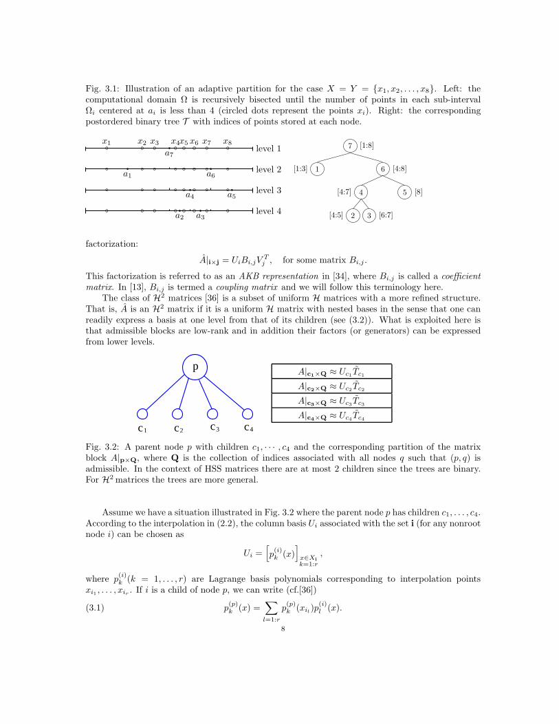
Fig. 3.1: Illustration of an adaptive partition for the case X = Y = x1, x2, . . . , x8. Left: thecomputational domain Ω is recursively bisected until the number of points in each sub-intervalΩi centered at ai is less than 4 (circled dots represent the points xi). Right: the correspondingpostordered binary tree T with indices of points stored at each node.

a1

a2 a3

a4 a5

a6

a7

level 4

level 3

level 2

level 1x1 x2 x3 x4x5 x6 x7 x8 7 [1:8]

6 [4:8]

5 [8]4[4:7]

3 [6:7]2[4:5]

1[1:3]

factorization:

A|i×j = UiBi,jVTj , for some matrix Bi,j .

This factorization is referred to as an AKB representation in [34], where Bi,j is called a coefficientmatrix. In [13], Bi,j is termed a coupling matrix and we will follow this terminology here.

The class of H2 matrices [36] is a subset of uniform H matrices with a more refined structure.That is, A is an H2 matrix if it is a uniform H matrix with nested bases in the sense that one canreadily express a basis at one level from that of its children (see (3.2)). What is exploited here isthat admissible blocks are low-rank and in addition their factors (or generators) can be expressedfrom lower levels.

c c c3c21 4

pA|c1×Q ≈ Uc1 Tc1

A|c2×Q ≈ Uc2 Tc2

A|c3×Q ≈ Uc3 Tc3

A|c4×Q ≈ Uc4 Tc4

Fig. 3.2: A parent node p with children c1, · · · , c4 and the corresponding partition of the matrixblock A|p×Q, where Q is the collection of indices associated with all nodes q such that (p, q) isadmissible. In the context of HSS matrices there are at most 2 children since the trees are binary.For H2 matrices the trees are more general.

Assume we have a situation illustrated in Fig. 3.2 where the parent node p has children c1, . . . , c4.According to the interpolation in (2.2), the column basis Ui associated with the set i (for any nonrootnode i) can be chosen as

Ui =[p(i)k (x)

]x∈Xi

k=1:r

,

where p(i)k (k = 1, . . . , r) are Lagrange basis polynomials corresponding to interpolation points

xi1 , . . . , xir . If i is a child of node p, we can write (cf.[36])

(3.1) p(p)k (x) =

∑

l=1:r

p(p)k (xil)p

(i)l (x).

8

The matrix version of (3.1) then leads to the so-called nested basis :

Up =

Uc1Rc1

...Uc4Rc4

, with Ri =

p(p)1 (xi1) . . . p

(p)r (xi1)

......

...

p(p)1 (xir ) . . . p

(p)r (xir )

.

The nested basis can also be obtained through algebraic compressions based on a bottom-upprocedure. Let A|p×Q denote the entire (numerically) low rank block row associated with nodep, i.e., Q is the union of all indices q such that (p, q) is admissible. As illustrated in Fig. 3.2,assuming that the column basis Uci has been obtained from a rank-r factorization of the submatrixA|ci×Q ≈ Uci Tci , we then derive

A|p×Q ≈

Uc1

Uc2

Uc3

Uc4

Tc1Tc2Tc3Tc4

.

Applying a rank-r factorization to the transpose of[T Tc1 T T

c2 T Tc3 T T

c4

]leads to

Tc1Tc2Tc3Tc4

≈

Rc1

Rc2

Rc3

Rc4

Tp −→ A|p×Q ≈ UpTp with Up =

Uc1Rc1

Uc2Rc2

Uc3Rc3

Uc4Rc4

.

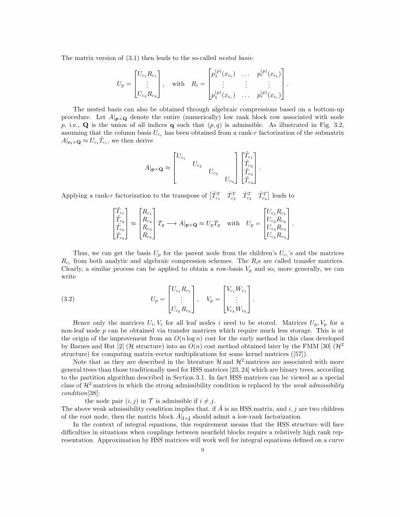
Thus, we can get the basis Up for the parent node from the children’s Uci ’s and the matricesRci from both analytic and algebraic compression schemes. The Ris are called transfer matrices.Clearly, a similar process can be applied to obtain a row-basis Vp and so, more generally, we canwrite

(3.2) Up =

Uc1Rc1

...UckRck

, Vp =

Vc1Wc1

...VckWck

.

Hence only the matrices Ui, Vi for all leaf nodes i need to be stored. Matrices Up, Vp for anon-leaf node p can be obtained via transfer matrices which require much less storage. This is atthe origin of the improvement from an O(n logn) cost for the early method in this class developedby Barnes and Hut [2] (H structure) into an O(n) cost method obtained later by the FMM [30] (H2

structure) for computing matrix-vector multiplications for some kernel matrices ([57]).Note that as they are described in the literature H and H2 matrices are associated with more

general trees than those traditionally used for HSS matrices [23, 24] which are binary trees, accordingto the partition algorithm described in Section 3.1. In fact HSS matrices can be viewed as a specialclass of H2 matrices in which the strong admissibility condition is replaced by the weak admissibilitycondition[38]:

the node pair (i, j) in T is admissible if i 6= j.The above weak admissibility condition implies that, if A is an HSS matrix, and i, j are two childrenof the root node, then the matrix block A|i×j should admit a low-rank factorization.

In the context of integral equations, this requirement means that the HSS structure will facedifficulties in situations when couplings between nearfield blocks require a relatively high rank rep-resentation. Approximation by HSS matrices will work well for integral equations defined on a curve

9

where kernel functions are discretized. In other cases the numerical rank of A|i×j may not necessar-ily be small even when a non-oscillatory kernel function is discretized on a surface or in a volume[13, 63].

The construction of H2 and HSS matrices involves computing the basis matrices U, V at the leaflevel, along with the transfer matrices R,W , and the coupling matrices B associated with a tree T .In particular, each leaf node i is assigned four matrices Ui, Vi, Ri,Wi and each nonleaf node i atlevel l ≥ 3 is assigned two matrices Ri,Wi.

There are two types of Bi,j matrices, those corresponding to the nearfield blocks at the leaflevel, and those corresponding to the coupling matrix where the product UiBi,jV

Tj approximates

block A|i×j for certain admissible (i, j). In general, the computation of Bi,j is more complicatedbecause one has to carefully specify the set of admissible node pairs (i, j) to be used for the efficientapproximation of A. If the distribution of points is uniform, the corresponding node pairs (i, j)are related to what is called interaction list in FMM [30, 57]. In more general settings where pointscan be arbitrarily distributed, they are called admissible leaves [13]. The set of admissible leavescorresponding to the minimal admissible partition [34] can be defined as follows:

L =(i, j) : i, j ∈ T are nodes at the same level such that (i, j) is admissible

but (pi, pj) is not admissible , where pi, pj are parents of i, j, respectively∪ (i, j) : i ∈ T is a leaf node and j ∈ T with lv(j) > lv(i) such that

(i, j) is admissible but (i, pj) is not admissible with pj the parent of j∪ (i, j) : j ∈ T is a leaf node and i ∈ T with lv(i) > lv(j) such that

(i, j) is admissible but (pi, j) is not admissible with pi the parent of i.

(3.3)

The node pairs (i, j) corresponding to blocks Bi,j that can not be compressed or partitioned, canbe identified through inadmissible leaves as defined below (cf.[13]):

(3.4) L− := (i, j) : i, j ∈ T are leaf nodes and (i, j) is not admissible .

In particular, for HSS matrices, it can be seen that L and L− have the following simple expression:

(3.5) L = (i, j) : i, j ∈ T and j = sibling of i, L− = (i, i) : i ∈ T is a leaf node.

This special feature will be used later (Section 3.3.1) to simplify the notation associated with HSSmatrices. The U, V,R,W,B matrices are called H2, or HSS, generators in the remaining sections.

3.3. Levelwise construction. Although the HSS structure may appear to be simpler thanthe H2 structure, based on their algebraic definitions the HSS construction procedure is actuallymore complex. This is because HSS matrices require the compression of both nearfield and farfieldblocks while H2 matrices only require the compression on farfield blocks. For example, if two sets Xi

and Yj are almost adjacent to each other (τ ≈ 1 in (2.3)), then the analytic approximation will notproduce a low rank, i.e., to get an accurate approximation, r has to be large in (2.6). In this case,the H2 matrix will form this block explicitly as a dense matrix while the HSS matrix still requiresthe block to be factorized. In what follows, we will first discuss SMASH for the HSS constructionin detail and then present the H2 construction with an emphasis on their differences.

3.3.1. HSS construction. Due to the simple structure of L,L− in (3.5), the notation denotingthe coupling matrices and nearfield blocks can be simplified in the HSS representation. Specifically,for (i, j) ∈ L, Bi,j can be represented as Bi with the second index j dropped because j = sibling of iis uniquely determined in a binary tree. An additional symbol Di is introduced to represent diagonalblocks Bi,i because (i, j) ∈ L− implies j = i.

10

Fig. 3.3: Illustration of the sets Ni used in HSS constructions.

N

N

SepSep

i

i, k i, k

k

ik

i

p

k ii k kleaf

pppp

Case 2 Case 1 Case 3

k

p i

p i

The basic idea of SMASH for the HSS construction is to first apply a truncated SVD to obtaina basis for nearfield blocks, use interpolation or expansion to obtain a basis for farfield blocks andthen apply SRRQR to the combination of these two bases to obtain the U, V,R and W matrices.The D and B matrices are submatrices of the original kernel matrix and their indices are readilyavailable after the computation of U, V,R,W matrices. In order to distinguish between column androw indices associated with a node i, we use superscript row to mark its row indices and col to markits column indices. For example, irow and icol denote the indices of points from X and Y containedin Ωi, respectively.

Assuming the HSS tree T has L levels, the HSS construction algorithm traverses T throughlevel l = L,L− 1, . . . , 2. Before the construction, two intermediate sets irow and icol are initializedas follows for each node i:

(3.6) irow =

irow if i is a leaf,

∅ otherwise,icol =

icol if i is a leaf,

∅ otherwise,

where the index sets irow and icol have been saved for each leaf node after the partition of Ω.Let Ni be the set of blocks that are nearfield to node i. .We set Ni = ∅ when i = root. For the

other cases, Ni is defined below where pi denotes the parent of i:

(3.7)Ni = k ∈ T such that : either k is a sibling of i

or pk ∈ Npiand (i, k) /∈ Sep

or k is a leaf such that k ∈ Npiand (i, k) /∈ Sep

,

where Sep denotes the set of all well-separated pairs of subdomains corresponding to a given partition:

(3.8) Sep := (i, j) : Ωi,Ωj are well-separated .

See Figure 3.3 for a pictorial illustration.Note that when i is a child of root then Npi

is empty and so only the first case can take place (kis a sibling of i). We also remark that the third case (k is a leaf such that k ∈ Np and (i, k) /∈ Sep)is required for non-uniform distributions and that it is empty if the distribution of the points isuniform. It is easy to see that if Ω = [0, 1] and X = Y is uniformly distributed, T is a perfect binarytree. In addition, if the separation ratio is set to τ = 0.5, then for any nonroot node i, Ni containsat most two nodes.

For each node i, let i denote the index set of the points in X ∩ Ωi. Similarly, j represents theindex set of the points in Y ∩ Ωj . Namely, Xi = X ∩ Ωi and Yj = Y ∩ Ωj .

Remark 3.1. Since the HSS structure [23, 24] is associated with a binary tree regardless of thedimension of the problem (see Section 3.2), to construct HSS matrices, bisection is used throughout

11

the adaptive partitions. For example, given a domain or a curve enclosed in a square in R2, we usebisection in the horizontal direction and the vertical direction alternatively in consecutive stages ofthe adaptive partitions, i.e., if horizontal bisection is used at partition level l, then vertical bisectionwill be employed at level l + 1. The numerical experiments in Section 6.3 and Section 6.4 provideillustrations. This partition strategy corresponds to the geometrically regular clustering (cf.[13]),and can be generalized into the geometrically balanced clustering (cf.[13]).

For each node i at level l, the construction algorithm first applies a truncated SVD to computean approximate column basis for the nearfield block rows in terms of Xirow :

(3.9) A−i :=

[A|irow×jcol

]j∈Ni

= SiΣ−i

[Sj

]

j∈Ni

+[E−

Σ |irow×jcol

]j∈Ni

,

where the columns of Si and [Sj ]j∈Niare the left/right singular vectors of A−

i and Σ−i is a diagonal

matrix composed of corresponding singular values of A−i such that the following estimate holds

(3.10) ‖E−Σ |irow×jcol‖F ≤

√|irow||jcol|ǫSVD‖A−

i ‖2, ∀ j ∈ Ni.

Here, ǫSVD is the relative tolerance used in the truncated SVD. The matrix Si is then taken as anapproximate column basis for the nearfield block rows A−

i .

For farfield blocks with respect to Xirow , a column basis Ui can be easily obtained throughinterpolation (2.2) or Taylor expansion (2.8) that only rely on Xirow and Ωi. Next, we apply SRRQRto the combined basis [Ui, Si] as shown below

(3.11) [Pi, Gi, irow] = compr([Ui, Si], i

row).

From these outputs, we set

(3.12)

Ui : = Pi

[IGi

]if i is a leaf node,

[Rc1

Rc2

]: = Pi

[IGi

]if i is a parent with children c1, c2.

Similarly, in order to compute V,W generators, a truncated SVD is first applied to the nearfieldblock columns (transposed) in terms of Yicol :

(3.13) A|i : =

[(Ajrow×icol

)T ]

j∈Ni

= TiΣ|i

[Tj

]

j∈Ni

+[(E

|Σ |jrow×icol)

T]

j∈Ni

,

where the truncation error satisfies

(3.14) ‖E|Σ |jrow×icol‖F ≤

√|icol||jrow|ǫSVD‖A|

i‖2, ∀ j ∈ Ni.

In the next step we compute a row basis Vi for the farfield blocks with respect to Yicol based on (2.2)or (2.8) and apply SRRQR to [Vi, Ti]:

[Fi, Hi, icol] = compr([Vi, Ti], i

col).

Then we set

(3.15)

Vi : = Fi

[IHi

]if i is a leaf node,

[Wc1

Wc2

]: = Fi

[IHi

]if i is a parent with children c1, c2.

12

Once the compressions for children nodes (at level l) are complete, we update the intermediate indexset associated with the parent node (at level l − 1) as shown below :

(3.16) prow = c1row ∪ c2

row, pcol = c1col ∪ c2

col,

where c1, c2 are the children of p.After the bottom-up traversal of T and hence the computation of U, V,R,W matrices, the B

and D matrices can be extracted as follows:

(3.17) Bi := A|irow×jcol

, j = sibling of i, and Di := A|irow×icol , i = leaf node.

3.3.2. H2 construction. As mentioned at the beginning of Section 3.3, the H2 constructionis simpler because nearfield blocks will not be factorized, and the only complication is that an H2

matrix may be associated with a more general tree structure where a parent can have more thantwo children.

SMASH for the H2 construction also follows a bottom-up levelwise traversal of T through levell = L,L− 1, . . . , 2. For each node i at level l, a column/row basis Ui/Vi corresponding to a farfieldblock row/column with index irow/icol can be obtained via either interpolation (2.2) or Taylorexpansion (2.8). The bases Ui and Vi are then passed into SRRQR

(3.18) [Pi, Gi, irow] = compr(Ui, i

row) and [Fi, Hi, icol] = compr(Vi, i

col).

The H2 generators U,R, V,W are then set as

(3.19)

Ui : = Pi

[IGi

]if i is a leaf node,

Rc1...

Rck

: = Pi

[IGi

]if i is a parent with children c1, . . . , ck,

Vi : = Fi

[IHi

]if i is a leaf node,

Wc1...

Wck

: = Fi

[IHi

]if i is a parent with children c1, . . . , ck.

Again, once the compressions for children nodes (at level l) are complete, the intermediate index setassociated with the parent node (at level l − 1) can be updated as in (3.16). Namely,

(3.20) prow = c1row ∪ · · · ∪ ck

row, pcol = c1col ∪ · · · ∪ ck

col, with children(p) = c1, . . . , ck.

Finally, analogous to (3.17), the coupling matrices associated with admissible leaves are extracted

based on index sets irow and jcol as

(3.21) Bi,j := A|irow×jcol

, ∀(i, j) ∈ L,

and the nearfield blocks associated with inadmissible leaves are formed by

(3.22) Bi,j := A|irow×jcol , ∀(i, j) ∈ L−.

Compared with standard H2 constructions based on either expansion or interpolation, SMASHis more efficient and easier to implement. First, in order to complete the H2 construction procedure,

13

it suffices to provide only the column/row basis for each farfield block, which can be easily obtainedbased on interpolation (2.2), for example, and the coupling matrices Bi,j can be simply extractedfrom the original matrix without resorting to any other formulas. Second, no information is requiredabout the translation to compute transfer matrices because the computation of R/W is essentiallythe same as that of U/V at leaf level. For all the children i of a node p, Ri/Wi are calculated jointlybased on a subset of points located inside Ωp (i.e., Xprow/Ypcol). Therefore, SMASH essentiallybuilds a hierarchy of grids and computes the bases at each level of the tree by repeating the sameoperations (3.18) on each coarse grid. In addition, the use of SRRQR guarantees that each entry ofthe U, V,R,W matrices is bounded by a user-specified constant, which ensures the numerical stabilityof the construction procedure. Note that the special structures in the nested bases (3.19) result innot only a reduced storage but also in faster matrix operations such as matrix-vector multiplications,linear system solutions, etc. Finally, since the computation of the basis matrices only relies on theinformation local to each node, as can be seen from (3.11) and (3.18), this construction algorithmis inherently suitable for a parallel computing environment.

3.4. Matrix-vector multiplication. Among various hierarchical rank structured matrix op-erations, the matrix-vector multiplication is the most widely used, as indicated by the popularity oftree code [2] (for H matrices) and fast multipole method [30, 57] (for H2 matrices).

The matrix-vector multiplication for an H2 matrix A follows first a bottom-up and then a top-down traversal of T [13, 34], which is a succinct algebraic generalization of the fast multipole method(cf.[57]). Suppose T has L levels, the node-wise version of this algorithm to evaluate z = Aq can besummarized as follows:

1. from level l = L to level l = 2, for each node i at level l, compute qi := V Ti q|icol if l = L;

otherwise, compute qi :=∑

c∈children(i)WTc qc;

2. for each nonroot node i ∈ T , compute zi =∑

j:(i,j)∈L Bi,j qj ;3. from level l = 2 to level l = L, for each node i at level l, if l < L, for each child c of i,

compute zc = zc +Rczi; otherwise, compute z|irow = Uizi +∑

j:(i,j)∈L−Bi,jq|jcol .

When X and Y are uniformly distributed in [0, 1]d, the resulting tree T is a perfect 2d-tree(each parent has 2d children and all leaf nodes are at the same level). If, in addition we assume theordering of points to be consistent with the postordering of tree T , i.e., for two siblings i, j ∈ T , ifi < j then the index of any point in box i must be smaller than point in box j, then an H2 matrixA has a telescoping representation:

A =B(L)+

U (L)

(U (L−1)

(. . .

(U (2)B(1)

(V (2)

)T+B(2)

). . .

)(V (L−1)

)T+B(L−1)

)(V (L)

)T,

(3.23)

where U (l), V (l) are block diagonal matrices:

(3.24) U (l) =

diag(Ui)lv(i)=l if l = L,

diag

Rc1

...

Rck

lv(i)=l

if l < L,V (l) =

diag(Vi)lv(i)=l if l = L,

diag

Wc1

...

Wck

lv(i)=l

if l < L,

and B(l) has a block structure. B(L) has #i ∈ T : lv(i) = L ×#i ∈ T : lv(i) = L blocks whereeach nonzero block corresponds to a nearfield block, while for l < L, there are #i ∈ T : lv(i) =l + 1 ×#i ∈ T : lv(i) = l + 1 blocks in B(l) and each nonzero block corresponds to a couplingmatrix. That is, in B(L), for lv(i) = lv(j) = L, block (li, lj) is equal to Bi,j if (i, j) ∈ L−; in B(l)

with l < L, for lv(i) = lv(j) = l + 1, block (li, lj) is equal to Bi,j if (i, j) ∈ L. Here li denotes the

14

location of node i at level l enumerated from left to right. If A is an HSS matrix associated with aperfect binary tree T , the structures of U (l) and V (l) are identical to those in (3.24) with k = 2 butB(l) has a much simpler block diagonal structure:

(3.25) B(l) =

diag(Di)i is a leaf node if l = L,

diag

([0 Bc1

Bc2 0

])

lv(i)=l

if l < L,

where c1 and c2 are the children of node i.Based on the explicit representation (3.23) of an H2 matrix associated with a perfect 2d-tree,

we can write down a levelwise version of the matrix-vector multiplication:1. at level l(2 ≤ l ≤ L), compute

(3.26) q(l) =(V (l)

)T. . .(V (L)

)Tq;

2. at level l(2 ≤ l ≤ L), compute

(3.27) z(l) = B(l−1)q(l);

3.

(3.28) z = B(L)q + U (L)(. . .(U (3)(U (2)z(2) + z(3)) + z(4)

)+ . . . z(L)

).

Notice that when X,Y are not uniformly distributed, T is not necessarily a perfect tree. Underthis condition, the nodes i, j corresponding to a coupling matrix Bi,j may not be at the same levelof T and the telescoping expansion (3.23) does not exist.

As for linear system solutions, H2 and HSS matrices take completely different approaches todirectly solve the resulting system. Linear complexity H2 matrix solvers ([13, 34]) heavily depend onrecursion to reduce the number of floating point operations while HSS matrices could benefit fromhighly parallelizable ULV-type algorithms (cf.[23], [24]) due to the special structure of HSS. However,as mentioned before, since the requirement of an HSS structure is too strong, the application of HSSmatrices is limited as compared to H2 matrices.

4. Error analysis. In this section, we analyze the approximation error of SMASH. Since theHSS construction is more complicated than H2 construction due to the factorization of nearfieldblocks, the corresponding error analysis is more involved. Here we first present error analysis forthe HSS construction associated with a perfect binary tree and then an error bound for the H2

construction associated with a perfect 2d-tree can be easily derived.For a perfect 2d-tree, it is natural and easy to interpret the levelwise construction in Section 3.3

in the following recursive manner:

(4.1) A(l) = U (l)A(l−1)(V (l)

)T+B(l) + E(l), ∀l ≥ 3,

where A(L) = A and A(l) (l < L) is a submatrix of A with the following block structure:

(4.2) (li, lj)−block of A(l) =

A|i×j if lv(i) = lv(j) = l and (i, j) is admissible,

0 if lv(i) = lv(j) = l and (i, j) is not admissible,

U (l), V (l), B(l) follow the definition in Section 3.4 and E(l) denotes the factorization error at levell. The superscripts row and col used in (3.6) are dropped in (4.2) in order to simplify the notation

15

used in the proof. Here, we assume that the items involving the index i refer to rows and the itemsinvolving the index j refer to columns. In addition, we introduce the notation

I(l) := ∪lv(i)=l i and J(l) := ∪lv(j)=l j.

Then the size of A(l) is equal to |I(l)| × |J(l)|.We also assume there exists a constant r(l) associated with each level such that

(4.3) |i| ≤ r(l), |j| ≤ r(l), i, j at level l, and r(l+1) ≤ r(l).

This constant r(l) is actually an upper bound for the numerical ranks in the admissible blocks atlevel l.

Expanding the recursion (4.1) leads to

A =U (L)

(U (L−1)

(. . .

(U (2)B(1)

(V (2)

)T+B(2) + E(2)

). . .

)(V (L−1)

)T

+B(L−1) + E(L−1))(

V (L))T

+B(L) + E(L).

(4.4)

Now we focus on the analysis of HSS approximation error. To estimate the norm of each diagonalblock in U (l) and V (l), the following lemma is needed, which is a simple consequence of SRRQR inTheorem 2.4 and thus holds for both H2 and HSS construction.

Lemma 4.1. Let s > 1 be the prescribed elementwise bound in SRRQR in Theorem 2.4, thenthe norms of the H2 generators in (3.19) or of the HSS generators in (3.12) and (3.15) satisfy thefollowing estimate

(4.5) ‖Pi

[IGi

]‖F ≤ s

√|i|r(l) and ‖Fj

[IHj

]‖F ≤ s

√|j|r(l),

for any nodes i, j at level l.

Proof. Under the assumption (4.3), we know that the column size of

[IGi

]is |i| ≤ r(l). Since

the row size of

[IGi

]is equal to |i| and the entries of Gi are bounded by s, we get

‖Pi

[IGi

]‖F ≤ s

√|i|+ (|i| − |i|)|i| ≤ s

√|i|r(l).

The same argument applies to ‖Fj

[IHj

]‖F .

In the following two lemmas, Lemma 4.2 and Lemma 4.3, we investigate the local error generatedin farfield approximation and nearfield approximation, respectively. Lemma 4.2 applies to both H2

and HSS construction, while Lemma 4.3 is only necessary for HSS construction because there is nonearfield approximation in H2 construction.

Lemma 4.2. Suppose i and j are two nodes at level l and (i, j) ∈ Sep. Denote the farfieldapproximation tolerance by ǫfar as in (2.9). Then the H2 generators computed in (3.19) or the HSSgenerators computed in (3.12) and (3.15) produce the following factorization

A|i×j = Pi

[IGi

]A|

i×j

(Fj

[IHj

])T

+ E(i,j),

16

where the approximation error E(i,j) satisfies

‖E(i,j)‖F ≤ 2s2√|i||j|r(l)ǫfar‖A|i×j‖F .

Proof. According to (2.7) and (2.11), we know that for each (i, j) ∈ Sep

A|i×j = UiBi,j VTj

+ EF |i×j = Pi

[IGi

]UiBi,j V

Tj

(Fj

[IHj

])T

+ EF |i×j

= Pi

[IGi

]A|

i×j

(Fj

[IHj

])T

+ E(i,j),

where

(4.6) E(i,j) := −Pi

[IGi

]EF |i×j

(Fj

[IHj

])T

+ EF |i×j.

Based on (2.9) and Lemma 4.1, we deduce that

‖E(i,j)‖F ≤ ‖Pi

[IGi

]‖F ‖EF |i×j

‖F ‖Fj

[IHj

]‖F + ‖EF |i×j‖F

≤ 2s√|i|r(l)ǫfar‖A|i×j‖F s

√|j|r(l) = 2s2

√|i||j|r(l)ǫfar‖A|i×j‖F .

Lemma 4.3. Suppose i and j are two nodes at level l of the HSS tree and (i, j) /∈ Sep. Thenin the HSS construction, the application of the truncated SVD with relative tolerance ǫSVD in (3.9)and (3.13) produces the following factorization

A|i×j = SiΣ−i Sj + E(i,j),

where

‖E(i,j)‖F ≤ s2 |j|√|i|r(l)r(l)ǫSVD‖A|

j‖F + s|i|√

|j|r(l)ǫSVD‖A−i ‖F .

Proof. According to (3.11), we know that

Si = Pi

[IGi

]Si |i.

Therefore,

SiΣ−i Sj = Pi

[IGi

]Si |iΣ−

i Sj

= Pi

[IGi

] (A|

i×j− E−

Σ |i×j

).

Based on (3.13), we further have:

A|i×j

= T Ti |

i(Σ

|j)

TT Tj + E

|Σ |i×j

.

17

Since

T Tj = (Tj |j)T

(Fj

[IHj

])T

,

we obtain

A|i×j

=(A|

i×j− E

|Σ |i×j

)(Fj

[IHj

])T

+ E|Σ |i×j

.

Therefore, we get

A|i×j = Pi

[IGi

]A|

i×j

(Fj

[IHj

])T

+ E(i,j),

where

(4.7) E(i,j) :=− Pi

[IGi

]E

|Σ |i×j

(Fj

[IHj

])T

+ Pi

[IGi

](E

|Σ |i×j − E−

Σ |i×j

)+ E−

Σ |i×j.

Introduce the notation

i := i \ i and j := j \ j,

we then have

E|Σ |i×j

= E|Σ |i×j

(Fj

[I0

])+ E

|Σ |i×j

(Fj

[0I

])and E−

Σ |i×j = Pi

[I0

]E−

Σ |i×j

+ Pi

[0I

]E−

Σ |i×j.

Substituting the above identities into (4.7), we obtain

(4.8)

E(i,j) =− Pi

[IGi

]E

|Σ |i×j

(Fj

[0Hj

])T

+ Pi

[IGi

]E

|Σ |i×j

(Fj

[0I

])T

− Pi

[0Gi

]E−

Σ |i×j

+ Pi

[0I

]E−

Σ |i×j.

Based on (3.10), (3.14) and Lemma 4.1, we have the estimate

‖E(i,j)‖F ≤ ‖[IGi

]‖F(‖Hj‖F ‖E|

Σ |i×j‖F + ‖E|

Σ |i×j‖F)+ ‖Gi‖F ‖E−

Σ |i×j

‖F + ‖E−Σ |i×j‖F

≤ ‖[IGi

]‖F√‖Hj‖2F + 1‖E|

Σ |i×j‖F +

√‖Gi‖2F + 1‖E−

Σ |i×j‖F

≤ s2 |j|√|i|r(l)r(l)ǫSVD‖A|

j‖F + s|i|√|j|r(l)ǫSVD‖A−

i ‖F .

Based on Lemmas 4.2–4.3, we can estimate the total approximation error at level l in HSSconstruction.

Lemma 4.4. Assume ǫSVD and ǫfar are the approximation tolerances used in the approximationof nearfield and farfield blocks in the HSS construction. Then the approximation error E(l) in (4.1)satisfies the following bound

‖E(l)‖F ≤ s22l/2+2(r(l+1)

)3/2 (r(l))3/2

ǫSVD‖A(l)‖F + 4s2r(l)r(l+1)ǫfar‖A(l)‖F ,18

where we have set r(L+1) := r(L).Proof. Based on Lemma 4.3, we know that the approximation error from the nearfield compres-

sion at level l can be estimated as follows:

∑

(i,j)/∈Sep

‖E(i,j)‖2F ≤ 2∑

(i,j)/∈Sep

(s4 |j|2 |i|

(r(l))3ǫ2SVD‖A|

j‖2F + s2 |i|2 |j|r(l)ǫ2SVD‖A−i ‖2F

)

≤ 2∑

i,j at level l

(s4 |j|2 |i|

(r(l))3ǫ2SVD‖A|

j‖2F + s2 |i|2 |j|r(l)ǫ2SVD‖A−i ‖2F

).

Since |i| ≤ 2r(l+1), |j| ≤ 2r(l+1) for nodes i, j at level l and there are 2l−1 nodes at this level, wefurther have

∑

(i,j)/∈Sep

‖E(i,j)‖2F ≤∑

i,j at level l

(2s4

(2r(l+1)

)3 (r(l))3ǫ2SVD‖A|

j‖2F + 2s2(2r(l+1)

)3r(l)ǫ2SVD‖A−

i ‖2F)

=∑

lv(i)=l

∑

lv(j)=l

2s4(2r(l+1)

)3 (r(l))3ǫ2SVD‖A|

j‖2F

+∑

lv(j)=l

∑

lv(i)=l

2s2(2r(l+1)

)3r(l)ǫ2SVD‖A−

i ‖2F

≤∑

lv(i)=l

2s4(2r(l+1)

)3 (r(l))3ǫ2SVD‖A(l)‖2F

+∑

lv(j)=l

2s2(2r(l+1)

)3r(l)ǫ2SVD‖A(l)‖2F

≤ 2l(s4(2r(l+1)

)3 (r(l))3

+ s2(2r(l+1)

)3r(l))ǫ2SVD‖A(l)‖2F

≤ s42l+4(r(l+1)

)3 (r(l))3ǫ2SVD‖A(l)‖2F .

Based on Lemma 4.2, we know that the approximation error for the farfield compression at level lsatisfies:

∑

(i,j)∈Sep

‖E(i,j)‖2F ≤∑

(i,j)∈Sep

(2s2√|i||j|r(l))2ǫ2far‖Ai×j‖2F .

Following the construction procedure (3.16) and the assumption (4.3), we have

|i| ≤ 2r(l+1), |j| ≤ 2r(l+1).(4.9)

Thus, we obtain the following estimation:

∑

(i,j)∈Sep

‖E(i,j)‖2F ≤∑

(i,j)∈Sep

(4s2r(l+1)r(l))2ǫ2far‖Ai×j‖2F

= 16s4(r(l+1)r(l))2ǫ2far∑

(i,j)∈Sep

‖Ai×j‖2F

≤ 16s4(r(l+1)r(l))2ǫ2far‖A(l)‖2F .19

To sum up both farfield and nearfield approximation errors, we obtain the estimate for the overallapproximation error introduced at level l:

‖E(l)‖F =

∑

(i,j)/∈Sep

‖E(i,j)‖2F +∑

(i,j)∈Sep

‖E(i,j)‖2F

1

2

≤ s22l/2+2(r(l+1)

)3/2 (r(l))3/2

ǫSVD‖A(l)‖F + 4s2r(l)r(l+1)ǫfar‖A(l)‖F .

The overall HSS approximation error in the Frobenius norm can then be derived in the followingtheorem.

Theorem 4.5. Suppose the HSS tree has L levels. With the assumptions in Lemma 4.4, SMASHproduces the following factorization

A =U (L)

(U (L−1)

(. . .

(U (2)B(1)

(V (2)

)T+B(2)

). . .

)(V (L−1)

)T

+B(L−1))(

V (L))T

+B(L) + E,

(4.10)

where the approximation error E satisfies the estimate

‖E‖F ≤ C1ǫSVD‖A‖F + C2ǫfar‖A‖F ,

with

C1 =L−1∑

l=2

2L+l/2+2s2L−2l+2(r(l+1) . . . r(L)

)2 (r(l+1)

)3/2 (r(l))5/2

C2 =L∑

l=2

2L+2s2L−2l+2(r(l)r(l+1) . . . r(L)

)2r(l+1).

Proof. According to (4.4), we know that the overall HSS approximation error E has the expres-sion

(4.11) E =(U (L) . . . U (3)

)E(2)

(V (L)) . . . V (3)

)T+ · · ·+ U (L)E(L−1)

(V (L)

)T+ E(L).

Note that the column size of(U (L) . . . U (l+1)

)is bounded by r(l)2l. Thus we have

(4.12) ‖U (L) . . . U (l+1)‖F ≤√r(l)2l‖U (L) . . . U (l+1)‖2 ≤ 2L/2sL−l

√r(l)r(l+1) . . . r(L),

20

and same upper bound holds for ‖V (L) . . . V (l+1)‖F . It follows from (4.11) that

(4.13)

‖E‖F ≤L−1∑

l=2

‖U (L) . . . U (l+1)‖F ‖E(l)‖F ‖V (L) . . . V (l+1)‖F + ‖E(L)‖F

≤L−1∑

l=2

2Ls2L−2lr(l)(r(l+1) . . . r(L)

)2s22l/2+2

(r(l+1)

)3/2 (r(l))3/2

ǫSVD‖A(l)‖F

+

L−1∑

l=2

2Ls2L−2lr(l)(r(l+1) . . . r(L)

)24s2r(l+1)r(l)ǫfar‖A(l)‖F + ‖E(L)‖F

≤L−1∑

l=2

2L+l/2+2s2L−2l+2(r(l+1) . . . r(L)

)2 (r(l+1)

)3/2 (r(l))5/2

ǫSVD‖A‖F

+

L∑

l=2

2L+2s2L−2l+2(r(l)r(l+1) . . . r(L)

)2r(l+1)ǫfar‖A‖F .

It is easy to see that the bound in (4.13) is quite pessimistic because we bound ‖A(l)‖F fromabove by ‖A‖F , where A(l) (defined in (4.2)) is a submatrix of A of size |I(l)| × |J(l)|.

Corollary 4.6. Besides the assumptions in Theorem 4.5, if there also exists a constant r ≥ 2such that r(l) ≤ r for each l > 1, then the approximation error E in SMASH satisfies the estimate:

‖E‖F ≤ (2r2s2)L(16ǫSVD + 8rǫfar)‖A‖F .

Next we estimate the error in H2 approximation. Note that, by setting ǫSVD = 0, the errorestimate in Theorem 4.5 also holds for the H2 construction with a possibly different constant C2

depending on dimension d. In fact, analogous to Lemma 4.4, we first have the following estimatefor the H2 construction:

‖E(l)‖F ≤ 4s2r(l)r(l+1)ǫfar‖A(l)‖F ,

where E(l) denotes the approximation error introduced at level l, as defined in (4.1). Assume theH2 matrix is associated with a perfect 2d-tree T (d ∈ 1, 2, 3), i.e., each nonleaf node of T has 2d

children and all leaves are at the same level. For a node i at level l, since |i| ≤ 2dr(l+1) ≤ 2dr(l), itfollows from (3.24), (3.19) and Lemma 4.1 that

‖U (l)‖2 ≤ s2d/2r(l).

Notice that the column size of(U (L) . . . U (l+1)

)is bounded by r(l)2dl. Then the counterpart of (4.12)

can be obtained for the H2 construction as:

‖U (L) . . . U (l+1)‖F ≤√r(l)2dl‖U (L) . . . U (l+1)‖2 ≤ 2dL/2sL−l

√r(l)r(l+1) . . . r(L),

and the same upper bound holds for ‖V (L) . . . V (l+1)‖F . The total approximation error can now be

21

obtained by means of (4.11):

‖E‖F ≤L−1∑

l=2

‖U (L) . . . U (l+1)‖F ‖E(l)‖F ‖V (L) . . . V (l+1)‖F + ‖E(L)‖F

≤L−1∑

l=2

2dLs2L−2lr(l)(r(l+1) . . . r(L)

)24s2r(l+1)r(l)ǫfar‖A(l)‖F + 4s2(r(L))2ǫfar‖A‖F

≤L−1∑

l=2

2dL+2s2L−2l+2(r(l)r(l+1) . . . r(L)

)2r(l+1)ǫfar‖A‖F + 4s2(r(L))2ǫfar‖A‖F

≤L∑

l=2

2dL+2s2L−2l+2(r(l)r(l+1) . . . r(L)

)2r(l+1)ǫfar‖A‖F .

The above error analysis yields the following theorem.Theorem 4.7. Suppose T is a perfect 2d-tree with L levels, associated with the H2 approxima-

tion of A. Under the assumptions in (4.3), SMASH produces the following factorization

A =U (L)

(U (L−1)

(. . .

(U (2)B(1)

(V (2)

)T+B(2)

). . .

)(V (L−1)

)T

+B(L−1))(

V (L))T

+B(L) + E,

(4.14)

where the approximation error E satisfies the estimate

‖E‖F ≤ Cǫfar‖A‖F ,

with

C =

L∑

l=2

2dL+2s2L−2l+2(r(l)r(l+1) . . . r(L)

)2r(l+1).

Corollary 4.8. Besides the assumptions in Theorem 4.7, if there also exists a constant r ≥ 2such that r(l) ≤ r for each l > 1, then the approximation error E in SMASH satisfies the estimate:

‖E‖F ≤ (2dr2s2)L8rǫfar‖A‖F .

Finally, we will show that the term (2dr2s2)L in Corollaries 4.6-4.8 can be bounded by functionsof n which are independent of ǫfar and ǫsvd under certain assumptions.

Proposition 4.9. Given r, let T be a perfect 2d-tree of L levels such that r2dL ≤ n. Assumewithout loss of generality that s ≤ 2. Then the constants in Corollary 4.6 and Corollary 4.8 satisfythe following estimation:

(4.15)(2dr2s2

)L ≤ n2

d+1+ 1

2dlog

2n.

Proof. Since r2dL ≤ n, we have L ≤ 1d log2

nr . It follows that

2dLs2L ≤ 2dL22L ≤(nr

) 2

d+1

≤ n2

d+1.

22

Next it remains to bound r2L ≤ r2

dlog

2

nr . To this end, we define g(x) = xlog2

nx for x ≥ 1. Then

r2L ≤ (g(r))2

d . It can be verified that the global maximum of g is achieved at x =√n. Therefore,

r2L ≤ (g(r))2

d ≤(g(√n)) 2

d = n1

2dlog

2n,

and (4.15) is proved. Proposition 4.9 also indicates that C1, C2 in Theorem 4.5 and C in The-orem 4.7 all can be bounded by constants which are independent of ǫfar and ǫsvd under certainassumptions.

5. Complexity analysis. This section studies the complexity of SMASH for an n×n matrix.For simplicity, we only consider the case when X = Y and the points are uniformly distributed.Under this assumption, a perfect tree T will be used for both HSS and H2 structures.

5.1. Complexity for the HSS construction. We start with the HSS construction case.Since the HSS matrix structure is only efficient for one dimensional problems, we will focus on theone-dimensional problems in this section. Suppose T has L levels such that n = O(r2L), where r isa positive integer such that the rank of HSS generators is bounded above by r and

(5.1) |irow| ≤ 2r, |icol| ≤ 2r, ∀i 6= root.

Notice that in the context of integral equations in potential theory, the assumption (5.1) in generalholds only for integral equations defined on a curve. Since the points are uniformly distributed, foreach nonroot node i, the number of nodes in Ni is very small, which we assume to be bounded aboveby 3. Under these assumptions, we have the following complexity estimate.

Theorem 5.1. Let T be a perfect binary tree with L levels and (5.1) hold. Then the complexityof SMASH for the HSS construction in Section 3.3.1 is O(n).

Proof. Based on (5.1), it is easy to see that, for each nonroot node i, the compression cost forits nearfield blocks in (3.9) is O(r3). This is because the size of the nearfield block row in (3.9) is nolarger than 2r-by-6r under the above assumption for Ni. Besides, the farfield basis matrix Ui hascolumn size at most r, so the cost of an SRRQR procedure in (3.11) is O(r3 logs r). Therefore, thecompression cost associated with each nonroot node i is O(r3 logs r) and the complexity of the HSSconstruction is O(2Lr3 logs r) = r2O(n) = O(n).

5.2. Complexity for the H2 construction. For the H2 construction case, we assume thatwhen X ⊂ Rd, T is a perfect 2d-tree with L levels such that n = O(r2dL) and r is a positive integersuch that the rank of H2 generators is bounded by r and

(5.2) |irow| ≤ r2d, |icol| ≤ r2d, ∀i 6= root.

The analysis here is simpler than that of the HSS construction in Section 5.1. Since each nodei only involves the compression of farfield basis Ui |irow ( as well as Vi |icol ), whose size is no largerthan r2d-by-r under the assumption (5.2), we deduce that the compression cost associated with eachnode is O(r3). As a result, the complexity of the H2 construction is O(2dLr3) = r2O(n). Thus weconclude:

Theorem 5.2. Let T be a perfect 2d-tree with L levels and (5.2) hold. Then the complexity ofSMASH for the H2 construction in Section 3.3.2 is O(n).

6. Numerical examples. In this section, we present numerical examples to illustrate theperformance of SMASH. All of the numerical results were performed in MATLAB R2014b on amacbook air with a 1.6 GHz CPU and 8 GB of RAM. The following notation is used throughoutthe section:

• n: the size of A;• tconstr: wall clock time for constructing A in seconds;

23

• tmatvec: wall clock time for multiplying A with a vector in seconds;• tsol: wall clock time for solving Ax = b in seconds;• ǫsvd: relative tolerance used in the truncated SVD for the nearfield compression;• rand([0, 1]): a random number sampled from the uniform distribution in [0, 1].

6.1. Choice of parameters. Since the quality of a degenerate approximation depends on theunderlying kernel function, there is no rule of thumb in general on choosing the parameters to satisfya prescribed tolerance. For completeness, here we present a heuristic approach that we use in allnumerical experiments on the choice of parameters.

Given a matrix A and a tolerance ǫ, suppose one wants to construct a hierarchical matrix A(H, H2, or HSS) such that ‖A− A‖max ≈ ǫ. Then the following approach is adopted to determineparameters τ, r.

The choice of separation ratio τ ∈ (0, 1) only depends on the dimension of the problem, soit is chosen first. We choose τ such that τ ≤ 0.7 and, in general, a slightly larger τ is preferredfor higher dimensional problems. For example, we choose τ = 0.6 for essentially one-dimensionalproblems, such as those in Section 6.3 and Section 6.4; we choose τ = 0.65 for problems in two orthree dimensions in Section 6.2.

Having chosen a separation ratio τ , we use the following function to determine the farfieldapproximation rank r used in constructing Ui, Vi (before the SRRQR postprocessing):

r =

⌊log ǫ/ log τ − 20⌋, if ǫ < 10−8,

⌊log ǫ/ log τ − 15⌋, if 10−8 ≤ ǫ < 10−6,

max⌊log ǫ/ log τ − 10⌋, 5 otherwise,

where ⌊x⌋ yields the largest integer less than or equal to x. For example, in Section 6.2.1, ǫ = 10−7,τ = 0.65, r = 22; in Section 6.3, ǫ = 10−8, τ = 0.6, r = 21; in Section 6.4, ǫ = 10−10, τ = 0.6,r = 25.

6.2. Construction and matrix-vector multiplication of H2 matrices. In this section,we perform numerical experiments to test the construction and matrix-vector multiplication of anH2 approximation associated with kernels in both two and three dimensions. A complicated three-dimensional geometry (see Figure 6.2) is presented to illustrate the robustness of the algorithm.

6.2.1. Two dimensions. We first consider the kernel in (2.1) with dx = 1. We chose X asa uniform m × m grid in [0, 1]2 and A = [κ(x, y)]x,y∈X . The computational domain [0, 1]2 wasrecursively divided into 4 subdomains until the number of the points inside each domain was lessthan or equal to 50. We embedded [0, 1]2 in the complex plane and used the truncated Taylorexpansion (2.4) with r = 22 terms and the separation ratio τ = 0.65 to compress farfield blocks.The error is measured by the relative error ‖Au−Au‖/‖Au‖, where u is a random vector of lengthn = m2 with entries generated by rand([0, 1]). This is because one of the main applications ofhierarchical matrices is used as an alternative of FMM to perform matrix-vector multiplications.The numerical results are reported in Table 6.1.

As can be seen from Table 6.1, SMASH for the H2 construction and the matrix-vector multi-plication described in Section 3.4 scale linearly, which is consistent with the complexity analysis inSection 5.

6.2.2. Three dimensions. We consider the following point distributions in three dimensions:• uniform distribution inside the unit cube;• uniform distribution on the unit sphere;• random distribution on a complicated triceratops geometry embedded in the cube [−100, 100]3

as shown in Figure 6.2 1,

1The datasets are from the point cloud tools http://www.geo.tuwien.ac.at/downloads/pg/pctools/pctools.html

24

Table 6.1: Numerical results for 2D test in Section 6.2.1

n = m2 ‖Au−Au‖/‖Au‖ tconstr tmatvec

1600 6.69× 10−13 0.52 0.026400 2.00× 10−12 1.97 0.0725600 3.65× 10−12 9.53 0.30102400 4.87× 10−12 39.47 1.18

Table 6.2: Numerical results for 3D triceratops example in Section 6.2.2

n ‖Au−Au‖/‖Au‖ tconstr tmatvec

10000 1.98× 10−6 9.12 0.1420000 3.83× 10−6 23.20 0.3840000 5.83× 10−6 50.39 0.7480000 7.20× 10−6 115.03 1.57

where the kernel function for the first two cases is κ(x, y) = 1|x−y| (x 6= y) with κ(x, x) = 1 and the

kernel for the third case is taken as κ(x, y) = log |x−y||x−y| (x 6= y) with κ(x, x) = 1. Note that the second

kernel function has a stronger singularity than the first one near x = y. The H2 approximation A isconstructed based on interpolation in three dimensions, where 5 Chebyshev points are used in eachdirection.

n ×104

0.5 1 1.5 2 2.5 3 3.5 4 4.5 5 5.5

tim

e/n

×10-3

0

1

2

3

4

5

6

time per degree of freedom v.s. matrix size

n ×104

1 2 3 4 5 6 7 8

tim

e/n

×10-3

0

0.5

1

1.5

2

2.5

3

time per degree of freedom v.s. matrix size

Fig. 6.1: Time per degree of freedom plot for 3D test: cube (left) and sphere (right)

The numerical results are presented in Figure 6.1 and Table 6.2. It is easily seen from Figure 6.1that, for each case, the time per degree of freedom roughly remains constant as matrix size increases,which implies O(n) construction cost. For the highly non-uniform triceratops geometry, Table 6.2demonstrates nearly linear cost in terms of the matrix size, since the corresponding tree T is nolonger perfect in this case.

6.3. Cauchy-like matrices. We consider in this section the numerical solution of Cauchy-likematrices. It is known that Cauchy-like matrices are related to other types of structured matricesincluding Toeplitz matrices, Vandermonde matrices, Hankel matrices and their variants [46, 48, 47,52, 49, 50]. Consider the kernel κ(x, y) = 1/(x − y), x 6= y ∈ C. Let xi, yj(i, j = 1 : n) be 2npairwise distinct points in C. The Cauchy matrix is then given by C = [κ(xi, yj)]i,j=1:n, which is

25

Fig. 6.2: The 3D triceratops geometry used for the numerical experiments in Table 6.2.

known to be invertible [21]. Given two matrices w, v ∈ Cn×p, the (i, j)-entry of a Cauchy-like matrixA associated with generators w, v is defined by [8]

(6.1) ai,j =1

xi − yj

p∑

l=1

wi,lvj,l.

For simplicity, we consider the case p = 2, i.e., w (as well as v) is composed of two column vectors.Denote by w1, w2, v1, v2 the column vectors in u, v, i.e., w = [w1, w2], v = [v1, v2]. It can be seenthat A can be written as

(6.2) A = diag(w1)Cdiag(v1) + diag(w2)Cdiag(v2).

Existing approaches for solving Cauchy or Cauchy-like linear systems associated with points inR mainly rely on some variants of Gaussian elimination with pivoting techniques. For example, fastO(n2) algorithms for solving Cauchy linear systems can be found in [18, 19, 25, 32], etc.; a superfastO(n log3 n) algorithm based on a sequential block Gaussian elimination process was proposed in[54]. The performance of most existing methods depends on the the distribution of point sets x, y.As pointed out in [19], if two sets of points x, y can not be separated, for example, when theyare interlaced, existing algorithms (for example, BP-type algorithm of [18]) suffer from backwardstability issues. Moreover, due to the use of pivoting techniques, the accuracy of existing algorithmsheavily depend on the ordering of points [18, 19] and the analysis is limited to the case when thepoints are in R.

Therefore, in view of the issues mentioned above, we assume xi, yj are mixed together such thatin adaptive partition (see Section 3.1), each box contains the same number of points from xi and yj .We also consider that xi, yj are distributed on a curve in R2 as illustrated in Fig. 6.4 to demonstratethat the algorithm is independent of the ordering of points and is applicable for points in C.

We construct the HSS approximation A to A using SMASH discussed in Section 3.3.1 and thensolve the linear system associated with A using a fast ULV factorization solver [24]. Due to thechoice of stable expansion in (2.4), arbitrarily high approximation accuracy can be achieved withoutstability issues [20].

Note that the HSS approximation to C can be readily obtained as in Section 3. Consequently,the HSS approximations to diag(w1)Cdiag(v1) and diag(w2)Cdiag(v2) can be derived by modifyingU, V,D generators, respectively. The sum of these two HSS representations is also an HSS matrixwhose generators can be easily obtained using the technique presented in [64] by merging the twosets of HSS generators. Hence the HSS approximation to A is derived.

26

In the first experiment, the point sets xknk=1, yknk=1 are chosen as follows:

(6.3) xk = k/(n+ 1), yk = xk + 10−7 ∗ rand([0, 1]), k = 1, . . . , n.

In the second experiment, the point sets are distributed on the curve illustrated in Fig. 6.3 that isparametrized by

γ(t) = e−πi/6 ∗ [(0.5 + sin(4πt)) cos(2πt) + i(0.5 + sin(4πt)) sin(2πt)] , t ∈ [0, 1],

and xknk=1, yknk=1 are given by

(6.4) xk = γ(k/(n+ 1)), yk = γ(xk + 10−7 ∗ rand([0, 1])), k = 1, . . . , n.

In the third experiment, the point set xknk=1 is on the snail geometry in C as illustrated in Fig.6.4 and the point set yknk=1 is given by

(6.5) yk = xk + 10−7 ∗ rand([0, 1]), k = 1, . . . , n.

For generators of this Cauchy-like matrix, i.e., w = [w1, w2], v = [v1, v2], we chose wl, vl(l = 1, 2)such that each entry in those vectors was given by rand([0, 1]). In order to solve the linear systemAu = b, we constructed an HSS approximation A to A in (6.2) by SMASH. 1D boxes (i.e., intervals)and 2D boxes (i.e., rectangles) are used in adaptive partition for point sets in (6.3) and (6.5),respectively. The right subfigures in Fig. 6.4 illustrate the adaptive partition using 2D boxes asdescribed in Remark 3.1. We chose separation ratio as τ = 0.6 and adaptive partition stopped whenthe number of points inside each box was less than or equal 50. The nearfield blocks were compressedthrough SVD with truncation tolerance 10−9. The exact solution was set to be a column vector uof length n with entries generated by rand([0, 1]), and the right-hand side b was formed by b = Au.

-1 -0.5 0 0.5 1

-1

-0.8

-0.6

-0.4

-0.2

0

0.2

0.4

0.6

0.8

1

-1 -0.5 0 0.5 1

-1

-0.8

-0.6

-0.4

-0.2

0

0.2

0.4

0.6

0.8

1

Fig. 6.3: Honeybee geometry used for the numerical experiments in Table 6.3. Left: Original curve;Right: Adaptive partition of the curve for the case when n = 12800 in Table 6.3.

The numerical results for three Cauchy-like matrix problems are reported in Table 6.3. FromTable 6.3, we see that the computational time for both construction and the solution scale linearly,and SMASH in Section 3.3.1 is quite robust with respect to complex geometries. Moreover, it canbe seen that SMASH is independent of the ordering of points.

6.4. Integral equations. In this section, we solve Laplace boundary value problems via theintegral equation method. Assume Ω is a smooth simply-connected domain in R2 and let Γ = ∂Ωbe the boundary of Ω of class C2. Consider the interior Dirichlet problem: find u ∈ C2(Ω) ∩ C(Ω)such that

(6.6)∆u = 0 in Ω,

u = uD on Γ,

27

-2.5 -2 -1.5 -1 -0.5 0 0.5 1 1.5

-1

-0.5

0

0.5

1

1.5

2

-2.5 -2 -1.5 -1 -0.5 0 0.5 1 1.5

-1

-0.5

0

0.5

1

1.5

2

2.5

Fig. 6.4: Snail geometry used for the numerical experiments in Table 6.3. Left: Original curve;Right: Adaptive partition of the curve for the case when n = 12800 in Table 6.3.

Table 6.3: Numerical results for solving the Cauchy-like matrix when xknk=1 are distributed onthree different curves.

curve n ‖u− u‖/‖u‖ ‖Au−Au‖/‖Au‖ tconstr tsol

[0, 1]

1600 7.69× 10−12 5.56× 10−15 0.33 0.113200 1.01× 10−09 3.87× 10−14 0.63 0.196400 5.58× 10−11 5.58× 10−14 1.29 0.3512800 1.47× 10−08 5.87× 10−14 2.58 0.69

honeybee

1600 9.37× 10−11 8.09× 10−14 1.14 0.283200 9.78× 10−10 5.60× 10−13 2.22 0.516400 1.55× 10−09 9.16× 10−13 4.42 0.9612800 2.76× 10−09 1.54× 10−12 8.49 1.87

snail

1600 2.65× 10−11 1.51× 10−15 1.58 0.363200 7.48× 10−11 1.82× 10−15 3.28 0.736400 8.38× 10−11 3.49× 10−15 6.46 1.4212800 3.86× 10−10 2.59× 10−15 11.82 2.64

where uD ∈ C(Γ) is given. With smooth boundary curves and Dirichlet data, the wellposedness ofthis problem is well studied in potential theory [40, 41].

The fundamental solution and its gradient (in terms of y) for the Laplace equation in R2 aregiven by:

Φ(x,y) = − 1

2πlog |x− y|, and ∇yΦ(x,y) = − 1

2π

y − x

|x− y|2 .

Let νy denote the unit outer normal at point y ∈ Γ. The double layer potential with continuousdensity σ is given by

(6.7) Kσ(x) :=

∫

Γ

∂Φ(x,y)

∂νyσ(y)dsy =

∫ 1

0

∂Φ(x, r(t))

∂νy|r′(t)|σ(r(t))dt, x ∈ Ω,

where we assume Γ is parametrized by r(t) : [0, 1] → R2.Given Dirichlet data uD ∈ C(Γ) in (6.6), we solve the following integral equation for σ ∈ C(Γ):

(6.8) (K − 1

2I)σ = uD, on Γ.

28

It is well-known ([41]) that the problem above for σ ∈ C(Γ) is well-posed, and the correspondingdouble layer potential u := Kσ solves the interior Dirichlet problem (6.6).

Denote the kernel in the second integral in (6.7) by

(6.9) κ(s, t) :=∂Φ(r(s), r(t))

∂νy|r′(t)|.

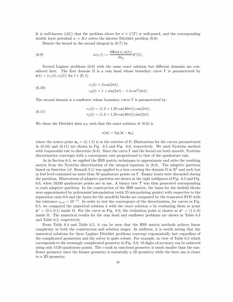
Several Laplace problems (6.6) with the same exact solution but different domains are con-sidered here. The first domain Ω is a ram head whose boundary curve Γ is parametrized byr(t) = (r1(t), r2(t)) for t ∈ [0, 1]:

(6.10)r1(t) = 2 cos(2πt),

r2(t) = 1 + sin(2πt)− 1.4 cos4(4πt).

The second domain is a sunflower whose boundary curve Γ is parametrized by:

(6.11)r1(t) = (1.3 + 1.25 cos(40πt)) cos(2πt),

r2(t) = (1.3 + 1.25 cos(40πt)) sin(2πt).

We chose the Dirichlet data uD such that the exact solution of (6.6) is

u(x) = log |x− x0|,

where the source point x0 = (2, 1.5) is in the exterior of Ω. Illustrations for the curves parametrizedin (6.10) and (6.11) are shown in Fig. 6.5 and Fig. 6.6, respectively. We used Nystrom methodwith trapezoidal rule to discretize (6.8). Since the curve Γ and the kernel are both smooth, Nystromdiscretization converges with a convergence rate proportional to that of the quadrature rule.

As in Section 6.3, we applied the HSS matrix techniques to approximate and solve the resultingmatrix from the Nystrom discretization of the integral equation in (6.8). The adaptive partitionbased on bisection (cf. Remark 3.1) was applied to a box covering the domain Ω in R2 and each boxin leaf level contained no more than 50 quadrature points on Γ. Empty boxes were discarded duringthe partition. Illustrations of adaptive partition are shown in the right subfigures of Fig. 6.5 and Fig.6.6, when 10240 quadrature points are in use. A binary tree T was then generated correspondingto each adaptive partition. In the construction of the HSS matrix, the bases for the farfield blockswere approximated by polynomial interpolation (with 25 interpolating points) with respective to theseparation ratio 0.6 and the bases for the nearfield blocks are computed by the truncated SVD withthe tolerance ǫsvd = 10−11. In order to test the convergence of the discretization, for curves in Fig.6.5, we compared the numerical solution u with the exact solution u by evaluating them at pointx∗ = (0.1, 0.1) inside Ω. For the curve in Fig. 6.6, the evaluation point is chosen as x∗ = (1.5, 0)inside Ω. The numerical results for the ram head and sunflower problems are shown in Table 6.4and Table 6.5, respectively.

From Table 6.4 and Table 6.5, it can be seen that the HSS matrix methods achieve linearcomplexity at both the construction and solution stages. In addition, it is worth noting that thenumerical solutions for these Laplace Dirichlet problems converge exponentially fast regardless ofthe complicated geometries and the solver is quite robust. For example, in view of Table 6.5 whichcorresponds to the seemingly complicated geometry in Fig. 6.6, 10 digits of accuracy can be achievedusing only 5120 quadrature points. The ǫ-rank in ram-head geometry is much smaller than the sun-flower geometry since the former geometry is essentially a 1D geometry while the later one is closerto a 2D geometry.

29

-2.5 -2 -1.5 -1 -0.5 0 0.5 1 1.5 2 2.5-1.5

-1

-0.5

0

0.5

1

1.5

2

-2.5 -2 -1.5 -1 -0.5 0 0.5 1 1.5 2 2.5-1.5

-1

-0.5

0

0.5

1

1.5

2

Fig. 6.5: Ram head domain for the Dirichlet problem (6.6) with source point and evaluation pointmarked as green ‘+’ and red ‘*’, respectively. Left: Original curve; Right: Adaptive partition of theram head boundary curve for the case when 10240 quadrature points are used in Table 6.4.

-2.5 -2 -1.5 -1 -0.5 0 0.5 1 1.5 2 2.5

-2.5

-2

-1.5

-1

-0.5

0

0.5

1

1.5

2

2.5

-2.5 -2 -1.5 -1 -0.5 0 0.5 1 1.5 2 2.5

-2.5

-2

-1.5

-1

-0.5

0

0.5

1

1.5

2

2.5

Fig. 6.6: Sunflower domain for the Dirichlet problem (6.6) with source point and evaluation pointmarked as green ‘+’ and red ‘*’, respectively. Left: Original curve; Right: Adaptive partition of thesunflower boundary curve for the case when 10240 quadrature points are used in Table 6.5.

6.5. Nearly optimal compression. In this section, we compare the exact numerical rankof the largest off-diagonal block of A with the approximation rank obtained from SMASH. Thenumerical results show that the approximation rank is nearly optimal in the sense that it differsfrom the exact numerical rank by a small constant that is roughly independent of the kernel andthe matrix size.

Definition 6.1 (ǫ-rank). Let σ1 ≥ σ2 ≥ · · · ≥ σr be singular values of a nonzero matrix A.Given a tolerance ǫ ∈ (0, 1), the relative ǫ-rank of a matrix A, denoted by rǫ(A), is the largest numberi such that σi ≥ ǫσ1.

Consider the numerical examples in Section 6.4, where different curves give rise to differentkernels according to (6.9). Let i, j be two children of the root node. We focus on the (largest)off-diagonal block Airow×jcol .

We consider three tolerances: ǫ = 10−3, 10−6, 10−10. We list the size of Airow×jcol , the exactǫ-rank, and the approximation rank characterized by the size of Bi generator with size(Bi) :=maximum between row size and column size. The results are reported in Table 6.6 .

Note that no a priori information is needed to determine the approximation rank as it is solelyderived from the prescribed tolerance and the construction algorithm. Thus the numerical resultsalso imply that the proposed method in Section 6.1 for choosing parameters is satisfactory.

6.6. Storage cost. In this section, we demonstrate the benefit of the special structure in thegenerators produced by SMASH. We store the HSS generators using the strategy mentioned at the

30

Table 6.4: Numerical results for solving a 2D Laplace Dirichlet problem in a ram head domain asshown in Fig. 6.5.

n |u(x∗)− u(x∗)| ‖A− A‖max cond(A) tconstr tsol160 5.03× 10−08 1.06× 10−10 6.15× 1001 0.42 0.107320 9.54× 10−11 6.81× 10−10 6.92× 101 1.54 0.042640 1.91× 10−12 7.98× 10−10 6.00× 101 2.93 0.1271280 8.22× 10−13 2.26× 10−09 6.02× 101 5.41 0.1032560 7.78× 10−13 3.90× 10−09 6.02× 101 9.76 0.1775120 1.50× 10−13 9.63× 10−09 6.02× 101 18.74 0.28210240 1.96× 10−12 1.01× 10−08 6.02× 1001 34.78 0.591

Table 6.5: Numerical results for solving a 2D Laplace Dirichlet problem in a sunflower domain asshown in Fig. 6.6.

n |u(x∗)− u(x∗)| ‖A− A‖max cond(A) tconstr tsol640 2.96× 10−02 1.20× 10−08 5.65× 103 5.42 0.1051280 1.25× 10−03 2.65× 10−08 2.23× 103 16.80 0.2562560 1.88× 10−06 3.56× 10−08 1.85× 103 41.76 0.6245120 1.02× 10−10 4.27× 10−07 1.72× 104 102.65 1.42910240 1.66× 10−11 3.80× 10−07 1.12× 104 192.78 2.16520480 8.03× 10−10 9.55× 10−07 6.86× 103 316.68 3.219

end of Section 2.3. For comparison, we also compute the cost by storing the generators as densematrices, denoted by HSS0, as well as the storage cost for the original dense matrix. The test matrixA of order 10240 is derived from kernels in Section 6.4 and all entries are stored in double precision.The results are collected in Table 6.7 for different geometries and different approximation accuracy.The reduction in storage justifies the use of strong rank-revealing QR algorithm in the constructionand we see that SMASH is quite cheap even when a high approximation accuracy is in use.

6.7. Storage comparison with H2 recompression algorithm. In this section, we providesome memory comparison between the SMASH H2 algorithm and the H2 recompression algorithmimplemented in H2Lib [9]. In order to do a fair comparison, we tested both algorithms on the samemachine, the same kernels (Newton, exponential and logarithmic kernels) and the same points. Bothalgorithms used the same interpolation method (5 interpolation points per direction) to obtain thebases for far field blocks. The recompression tolerance was set to be 10−4 in both algorithms, whichresulted in O(10−6) relative error (measured as ‖Au−Au‖/‖Au‖) for matrix-vector products, usingdouble precision data types.

It can be seen from Tables 6.8–6.10 that the SMASH H2 algorithm results in less memory inmost experiments except the exponential kernel test with 5× 105 points and the logarithmic kerneltests with 5×105 and 2×106 points. The other main difference between these two algorithms is thatthe SMASH algorithm in general has much smaller peak memory usage. For example, the SMASHalgorithm has the peak memory of 14.75GB for the logarithmic kernel with 4× 106 points while theH2Lib uses 47.92GB peak memory.

7. Conclusion. We presented a unified framework, called SMASH, to construct either ann × n HSS or H2 matrix with an O(n) cost. One appealing feature of this scheme is its simpleimplementation which only requires a routine to compress far field blocks. In addition, SMASH can

31

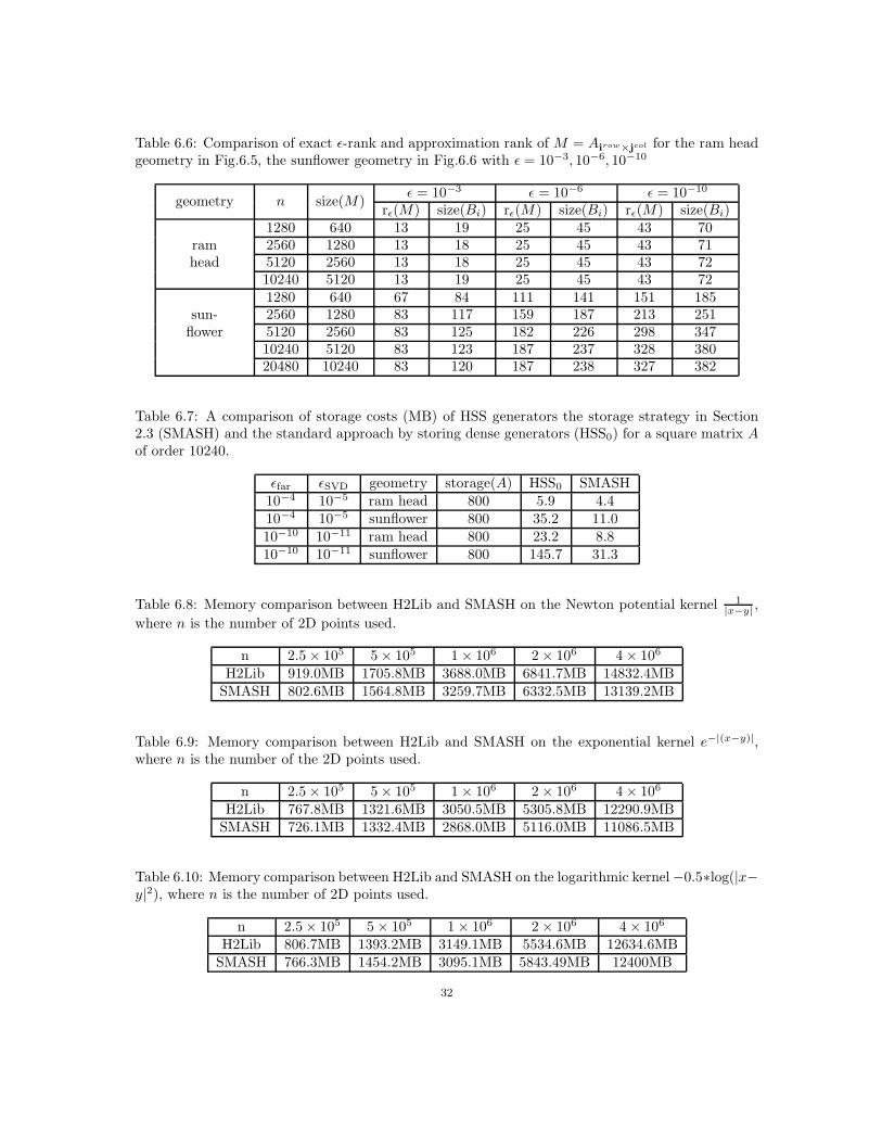
Table 6.6: Comparison of exact ǫ-rank and approximation rank of M = Airow×jcol for the ram headgeometry in Fig.6.5, the sunflower geometry in Fig.6.6 with ǫ = 10−3, 10−6, 10−10

geometry n size(M)ǫ = 10−3 ǫ = 10−6 ǫ = 10−10

rǫ(M) size(Bi) rǫ(M) size(Bi) rǫ(M) size(Bi)

ramhead

1280 640 13 19 25 45 43 702560 1280 13 18 25 45 43 715120 2560 13 18 25 45 43 7210240 5120 13 19 25 45 43 72

sun-flower

1280 640 67 84 111 141 151 1852560 1280 83 117 159 187 213 2515120 2560 83 125 182 226 298 34710240 5120 83 123 187 237 328 38020480 10240 83 120 187 238 327 382

Table 6.7: A comparison of storage costs (MB) of HSS generators the storage strategy in Section2.3 (SMASH) and the standard approach by storing dense generators (HSS0) for a square matrix Aof order 10240.

ǫfar ǫSVD geometry storage(A) HSS0 SMASH10−4 10−5 ram head 800 5.9 4.410−4 10−5 sunflower 800 35.2 11.010−10 10−11 ram head 800 23.2 8.810−10 10−11 sunflower 800 145.7 31.3

Table 6.8: Memory comparison between H2Lib and SMASH on the Newton potential kernel 1|x−y| ,

where n is the number of 2D points used.

n 2.5× 105 5× 105 1× 106 2× 106 4× 106

H2Lib 919.0MB 1705.8MB 3688.0MB 6841.7MB 14832.4MBSMASH 802.6MB 1564.8MB 3259.7MB 6332.5MB 13139.2MB

Table 6.9: Memory comparison between H2Lib and SMASH on the exponential kernel e−|(x−y)|,where n is the number of the 2D points used.

n 2.5× 105 5× 105 1× 106 2× 106 4× 106

H2Lib 767.8MB 1321.6MB 3050.5MB 5305.8MB 12290.9MBSMASH 726.1MB 1332.4MB 2868.0MB 5116.0MB 11086.5MB

Table 6.10: Memory comparison between H2Lib and SMASH on the logarithmic kernel−0.5∗log(|x−y|2), where n is the number of 2D points used.

n 2.5× 105 5× 105 1× 106 2× 106 4× 106

H2Lib 806.7MB 1393.2MB 3149.1MB 5534.6MB 12634.6MBSMASH 766.3MB 1454.2MB 3095.1MB 5843.49MB 12400MB

32

greatly reduce the memory cost relative to existing analytic construction schemes. The numericalexperiments illustrated the efficiency and robustness of SMASH through a few examples with variouspoint distributions and kernel matrices.

We plan to extend this scheme to highly oscillatory kernels and to develop approximate inverse-type preconditioners for solving the resulting linear systems with H2 matrix representations.

Acknowledgments. We would like to thank anonymous referees for their useful suggestionswhich led to substantial improvements of the original version of this paper. YX would like to thankProf. Ming Gu for fruitful discussions about the strong rank revealing QR algorithm and Prof.Steffen Borm for his kind explanation of the new developments of H2 matrices and providing uswith a kernel matrix interface for his H2Lib package[9].

REFERENCES

[1] C. R. Anderson, An implementation of the fast multipole method without multipoles, SIAM J. Sci. Statist.Comput., 13 (1992), pp. 923–947.

[2] J. Barnes and P. Hut, A hierarchical O(N log N) force-calculation algorithm, Nature, 324 (1986), pp. 446–449.[3] M. Bebendorf, Approximation of boundary element matrices, Numer. Math., 86 (2000), pp. 565–589.[4] , Hierarchical Matrices: A Means to Efficiently Solve Elliptic Boundary Value Problems, Lecture Notes

in Computational Science and Engineering, Springer Berlin Heidelberg, 2008.[5] M. Bebendorf and S. Rjasanow, Adaptive low-rank approximation of collocation matrices, Computing, 70

(2003), pp. 1–24.[6] M. Bebendorf and R. Venn, Constructing nested bases approximations from the entries of non-local operators,

Numer. Math., 121 (2012), pp. 609–635.[7] P. Benner and T. Mach, Computing all or some eigenvalues of symmetric Hl-matrices, SIAM J. Sci. Comput.,

34 (2012), pp. A485–A496.[8] D. A. Bini, B. Meini, and F. Poloni, Fast solution of a certain riccati equation through cauchy-like matrices.,

ETNA. Electronic Transactions on Numerical Analysis [electronic only], 33 (2008), pp. 84–104.[9] S. Borm, H2lib. http://www.h2lib.org/.

[10] , Approximation of integral operators by H2-matrices with adaptive bases, Computing, 74 (2005), pp. 249–271.

[11] S. Borm, Data-sparse approximation of non-local operators by h2-matrices, Linear Algebra Appl., 422 (2007),pp. 380–403.

[12] , Construction of data-sparse H2-matrices by hierarchical compression, SIAM J. Sci. Comput., 31 (2009),pp. 1820–1839.

[13] S. Borm, Efficient numerical methods for non-local operators : H2 -matrix compression, algorithms and anal-ysis, EMS Tracts in Mathematics, European Mathematical Society, Zurich, 2010.

[14] S. Borm and S. Christophersen, Approximation of integral operators by green quadrature and nested crossapproximation, Numerische Mathematik, 133 (2016), pp. 409–442.

[15] S. Borm and L. Grasedyck, Hybrid cross approximation of integral operators, Numer. Math., 101 (2005),pp. 221–249.

[16] S. Borm, L. Grasedyck, and W. Hackbusch, Introduction to hierarchical matrices with applications, ENG.ANAL. BOUND. ELEM., 27 (2003), pp. 405–422.

[17] S. Le Borne and L. Grasedyck, H-matrix preconditioners in convection-dominated problems, SIAM J. MatrixAnal. Appl., 27 (2006), pp. 1172–1183.

[18] T. Boros, T. Kailath, and V. Olshevsky, A fast parallel BjorckPereyra-type algorithm for solving Cauchylinear equations, Linear Algebra Appl., 302 (1999), pp. 265–293.

[19] , Special issue on structured and infinite systems of linear equations pivoting and backward stability offast algorithms for solving Cauchy linear equations, Linear Algebra Appl., 343 (2002), pp. 63–99.

[20] D. Cai and J. Xia, A stable and efficient matrix version of the fast multipole method, to be submitted.[21] D. Calvetti and L. Reichel, Factorizations of Cauchy matrices, J. Comput. Appl. Math., 86 (1997), pp. 103–

123.[22] J. Carrier, L. Greengard, and V. Rokhlin, A fast adaptive multipole algorithm for particle simulations,

SIAM Journal on Scientific and Statistical Computing, 9 (1988), pp. 669–686.[23] S. Chandrasekaran, M. Gu, and W. Lyons, A fast adaptive solver for hierarchically semiseparable represen-

tations, CALCOLO, 42 (2005), pp. 171–185.[24] S. Chandrasekaran, M. Gu, and T. Pals, A fast ULV decomposition solver for hierarchically semiseparable

representations, SIAM J. Matrix Anal. Appl., 28 (2006), pp. 603–622.

33

[25] I. Gohbert, T. Kailath, and V. Olshevsky, Fast Gaussian elimination with partial pivoting for matriceswith displacement structure, Math. Comput., 64 (1995), pp. 1557–1576.

[26] S.A. Goreinov, E.E. Tyrtyshnikov, and N.L. Zamarashkin, A theory of pseudoskeleton approximations,Linear Algebra Appl., 261 (1997), pp. 1–21.

[27] S. A. Goreinov, E. E. Tyrtyshnikov, and A. Yu. Yeremin, Matrix-free iterative solution strategies for largedense linear systems, Numer. Linear Algebra Appl., 4 (1997), pp. 273–294.

[28] L. Grasedyck, Existence of a low rank or -matrix approximant to the solution of a sylvester equation, Numer.Linear Algebra Appl., 11 (2004), pp. 371–389.

[29] L. Grasedyck, W. Hackbusch, and N. B. Khoromskij, Solution of large scale algebraic matrix riccati equa-tions by use of hierarchical matrices, Computing, 70 (2003), pp. 121–165.

[30] L. Greengard and V. Rokhlin, A fast algorithm for particle simulations, J. Comput. Phys., 73 (1987),pp. 325–348.

[31] M. Gu, Subspace iteration randomization and singular value problems, preprint.[32] M. Gu, Stable and efficient algorithms for structured systems of linear equations, SIAM J. Matrix Anal. Appl.,

19 (1998), pp. 279–306.[33] M. Gu and S. C. Eisenstat, Efficient algorithms for computing a strong rank-revealing QR factorization, SIAM

J. Sci. Comput., 17 (1996), pp. 848–869.[34] W. Hackbusch, Hierarchical matrices : algorithms and analysis, Springer, 2015.[35] W. Hackbusch and S. Borm, Data-sparse approximation by adaptive H2-matrices, Computing, 69 (2002),

pp. 1–35.[36] , H2-matrix approximation of integral operators by interpolation, Appl. Numer. Math., 43 (2002), pp. 129–

143.[37] W. Hackbusch, B.N. Khoromskij, and S.A. Sauter, On H2-matrices, in Lectures on applied mathematics,

Hans-Joachim Bungartz, Ronald H. W. Hoppe, and Christoph Zenger, eds., Springer, Berlin, 2000, pp. 9–29.[38] W. Hackbusch, B. N. Khoromskij, and R. Kriemann, Hierarchical matrices based on a weak admissibility

criterion, Computing, 73 (2004), pp. 207–243.[39] N. Halko, P. G. Martinsson, and J. Tropp, Finding structure with randomness: Probabilistic algorithms for

constructing approximate matrix decompositions, SIAM Review, 53 (2011).[40] G. C. Hsiao and W. L. Wendland, Boundary integral equations, Applied Mathematical Sciences, Springer,

Berlin, Heidelberg, 2008.[41] R. Kress, Linear Integral Equations, Applied Mathematical Sciences, Springer New York, 2013.[42] L. Lin, J. Lu, and L. Ying, Fast construction of hierarchical matrix representation from matrixvector multi-

plication, J. Comput. Phys., 230 (2011), pp. 4071–4087.[43] X. Liu, J. Xia, and M. V. de Hoop, Parallel randomized and matrix-free direct solvers for large structured

dense linear systems, SIAM J. Sci. Comput., 38 (2016), pp. S508–S538.[44] P.G. Martinsson and V. Rokhlin, A fast direct solver for boundary integral equations in two dimensions, J.

Comput. Phys., 205 (2005), pp. 1–23.[45] P. G. Martinsson, A fast randomized algorithm for computing a hierarchically semiseparable representation of

a matrix, SIAM J. Matrix Anal. Appl., 32 (2011), pp. 1251–1274.[46] V. Y. Pan, Structured Matrices and Polynomials: Unified Superfast Algorithms, Springer-Verlag New York,

Inc., New York, NY, USA, 2001.[47] , Fast Approximate Computations with Cauchy Matrices, Polynomials and Rational Functions, Springer

International Publishing, Cham, 2014, pp. 287–299.[48] V. Y. Pan, Transformations of matrix structures work again, Linear Algebra and its Applications, 465 (2015),

pp. 107–138.[49] , How Bad Are Vandermonde Matrices?, SIAM J. Matrix Anal. Appl., 37 (2016), pp. 676–694.[50] , Fast approximate computations with cauchy matrices and polynomials, Math. Comput., 86 (2017),

pp. 2799–2826.[51] V. Y. Pan, Q. Luan, J. Svadlenka, and L. Zhao, Primitive and cynical low rank approximation, preprocessing

and extensions, arXiv, (2016).[52] V. Y. Pan and X. Wang, Inversion of displacement operators, SIAM Journal on Matrix Analysis and Applica-

tions, 24 (2003), pp. 660–677.[53] V. Y. Pan and L. Zhao, Low-rank approximation of a matrix: Novel insights, new progress, and extensions,

arXiv, (2015).[54] V. Y. Pan and A. Zheng, Superfast algorithms for Cauchy-like matrix computations and extensions, Linear

Algebra Appl., 310 (2000), pp. 83–108.[55] V. Rokhlin, Rapid solution of integral equations of classical potential theory, Journal of Computational Physics,

60 (1985), pp. 187–207.[56] F.-H. Rouet, X. S. Li, P. Ghysels, and A. Napov, A distributed-memory package for dense hierarchically

semi-separable matrix computations using randomization, submitted to ACM Trans. Math. Softw.[57] X. Sun and N.P. Pitsianis, A matrix version of the fast multipole method, SIAM Rev., 43 (2001), pp. 289–300.[58] E. Tyrtyshnikov, Mosaic-skeleton approximations, CALCOLO, 33 (1996), pp. 47–57.

34

[59] , Incomplete cross approximation in the mosaic-skeleton method, Computing, 64 (2000), pp. 367–380.[60] Y. Xi and J. Xia, On the stability of some hierarchical rank structured matrix alogrithms, SIAM J. Matrix

Anal. Appl., 37 (2016), pp. 1279–1303.[61] Y. Xi, J. Xia, S. Cauley, and V. Balakrishnan, Superfast and stable structured solvers for toeplitz least

squares via randomized sampling, SIAM J. Matrix Anal. Appl., 35 (2014), pp. 44–72.[62] Y. Xi, J. Xia, and R. Chan, A fast randomized eigensolver with structured ldl factorization update, SIAM J.

Matrix Anal. Appl., 35 (2014), pp. 974–996.[63] J. Xia, Multi-layer hierarchical structures and factorizations, submitted to SIAM J. Matrix Anal. Appl.[64] , On the complexity of some hierarchical structured matrix algorithms, SIAM Journal on Matrix Analysis

and Applications, 33 (2012), pp. 388–410.[65] , Efficient structured multifrontal factorization for general large sparse matrices, SIAM J. Sci. Comput.,

35 (2013), pp. A832–A860.[66] J. Xia, S. Chandrasekaran, M. Gu, and X. S. Li, Fast algorithms for hierarchically semiseparable matrices,

Numer. Linear Algebra Appl., 17 (2010), pp. 953–976.[67] J. Xia, Y. Xi, and M. Gu, A superfast structured solver for Toeplitz linear systems via randomized sampling,

SIAM J. Matrix Anal. Appl., 33 (2012), pp. 837–858.[68] L. Ying, G. Biros, and D. Zorin, A kernel-independent adaptive fast multipole algorithm in two and three

dimensions, J. Comput. Phys., 196 (2004), pp. 591–626.

35