smoothed and corrected score approach to censored...
TRANSCRIPT

Smoothed and Corrected Score Approach to Censored
Quantile Regression With Measurement Errors
Yuanshan Wu, Yanyuan Ma, and Guosheng Yin∗
Abstract
Censored quantile regression is an important alternative to the Cox proportional hazards
model in survival analysis. In contrast to the usual central covariate effects, quantile re-
gression can effectively characterize the covariate effects at different quantiles of the survival
time. When covariates are measured with errors, it is known that naively treating mis-
measured covariates as error-free would result in estimation bias. Under censored quantile
regression, we propose smoothed and corrected estimating equations to obtain consistent
estimators. We establish consistency and asymptotic normality for the proposed estimators
of quantile regression coefficients. Compared with the naive estimator, the proposed method
can eliminate the estimation bias under various measurement error distributions and model
error distributions. We conduct simulation studies to examine the finite-sample properties
of the new method and apply it to a lung cancer study.
KEY WORDS: Censored data; Check function; Corrected estimating equation; Measure-
ment error; Kernel smoothing; Regression quantile; Semiparametric method; Survival anal-
ysis.
Short title: Measurement error censored quantile regression
∗Yuanshan Wu is Assistant Professor, School of Mathematics and Statistics, Wuhan University, Wuhan,Hubei 430072, China (E-mail: [email protected]). Yanyuan Ma is Professor, Department of Statistics,University of South Carolina, Columbia, SC 29208, U.S.A. (E-mail: [email protected]). GuoshengYin, the corresponding author, is Professor, Department of Statistics and Actuarial Science, The Universityof Hong Kong, Pokfulam Road, Hong Kong (E-mail: [email protected]). We thank two referees, the associateeditor and editor for their many constructive comments that have led to significant improvements in thearticle. Wu’s research was partially supported by National Natural Science Foundation of China, Ma’sresearch by National Science Foundation and National Institute of Neurological Disorder and Stroke, andYin’s research by the Research Grants Council of Hong Kong.
1
1 Introduction
Mean-based regression models have been extensively studied for randomly censored survival
data. For example, the Cox (1972) proportional hazards model characterizes the hazard
as a function of different covariates; and the accelerated failure time (AFT) model directly
formulates linear regression between the logarithm of the failure time and covariates. How-
ever, neither the Cox nor the AFT model can differentiate the covariate effect at higher or
lower quantiles of survival times, as they only provide the mean effect. In particular, the
AFT model concerns only the mean regression, for which the estimation procedure is typi-
cally based on the least squares or rank methods (Prentice, 1978; Buckley and James, 1979;
Ritov, 1990; Tsiatis, 1990; Wei, Ying, and Lin, 1990; Lai and Ying, 1991; and Jin et al.,
2003). On the other hand, quantile regression provides a robust alternative to mean-based
regression models. Under this framework, we can model the median or any other quantile
of the outcome or survival time (Koenker and Bassett, 1978; and Koenker, 2005). Regres-
sion parameters are often estimated by minimizing a check function, and the corresponding
variance estimates are typically obtained by resampling methods, such as bootstrap. When
censoring times are assumed to be fixed and known, quantile regression has been extensively
studied, particularly in the field of econometrics; for example, see Powell (1984), Buchinsky
and Hahn (1998), Fitzenberger (1997), and Khan and Powell (2001). In survival analysis
with random censoring, censored quantile regression (CQR) has been proposed and is gain-
ing much popularity (Ying, Jung, and Wei, 1995; Lindgren, 1997; Yang, 1999; Koenker and
Geling, 2001; Bang and Tsiatis, 2002; Chernozhukov and Hong, 2002; Portnoy, 2003; Peng
and Huang, 2008; and Wang and Wang, 2009).
In practice, covariates are often subject to measurement errors. The most common mea-
surement error structure is W = Z + U, where W is the observed surrogate, Z is the true
but unobserved covariate, and U is the random measurement error. For a comprehensive
coverage of various measurement error models and inference procedures with mean-based
regression, see Carroll et al. (2006). In the context of quantile regression with measurement
2
errors, Brown (1982) examined median regression and described the difficulty involved in
parameter estimation. He and Liang (2000) proposed root-n consistent estimators for linear
and partially linear quantile regression models. Their method assumes that the random error
in the response and the measurement errors in the covariates follow a spherical symmetric
distribution. Wei and Carroll (2009) proposed a novel approach to quantile regression with
measurement errors by utilizing the derivative property of the quantile function when the
same quantile regression structure is assumed for all the quantile levels. Recently, Wang, Ste-
fanski, and Zhu (2012) developed a corrected-loss function for the smoothed check function,
a substantial advance in this area. However, there is limited research on quantile regression
with covariate measurement errors under censoring. Ma and Yin (2011) studied covariate
measurement errors in CQR models based on the inverse probability weighting scheme, but
their method also requires the spherically symmetric distribution. In this paper, we study
the issue of covariate measurement errors in quantile regression with randomly censored
data. We propose a smoothed and corrected martingale-based estimating equation, consider
grid-based estimates for the quantile regression coefficients, and establish the asymptotic
properties of the proposed estimator by employing empirical process theory. Our proposed
method allows an abundant class of distributions for the error in the response; for example, it
could be light- or heavy-tailed, symmetric or asymmetric, homoscedastic or heteroscedastic.
The rest of the article is organized as follows. In Section 2, we describe the CQR model
with measurement errors, develop a corrected estimating equation based on a kernel smooth-
ing approximation, and establish the asymptotic properties of the resultant estimator. Sec-
tion 3 contains simulation studies for the evaluation of the finite sample performance of the
proposed method. A data set concerning lung cancer is analyzed in Section 4 and some con-
cluding remarks are provided in Section 5. The assumptions that we imposed in the paper
were listed and discussed in the Appendix and the detailed proofs of theorems are deferred
to the online Supplementary Material.
3

2 CQR Model With Measurement Errors
2.1 Model Specification
Let T denote the transformed failure time under a known monotone transformation, e.g.,
the logarithm function. Let C denote the censoring time under the same transformation.
Let Z be a p-vector of covariates, X = T ∧ C be the observed time, and ∆ = I(T ≤ C)
be the censoring indicator, where a ∧ b is the minimum of a and b, and I(·) is the indicator
function. Assume that T and C are conditionally independent given covariate Z.
For τ ∈ (0, 1), the conditional τth quantile function of survival time T given covariate Z
is defined as QT (τ |Z) = inf{t: P (T ≤ t|Z) ≥ τ}. The quantile regression model associated
with covariate Z has the form
QT (τ |Z) = ZTβ(τ), (2.1)
where β(τ) is an unknown p-vector of regression coefficients, representing the effect of Z on
the τth quantile of the transformed survival time.
In reality covariate Z may be measured with errors, so that we do not directly observe
Z but its surrogate W. We assume the classical error structure
W = Z + U,
where U is a p-variate random vector with mean 0 and covariance matrix Σ. The case
that some covariates are error-free is accommodated in our model by setting the relevant
terms in Σ to be zero. We further make the typical surrogacy assumption that (T, C) and
W are conditionally independent given covariate Z. For ease of exposition, we assume Σ
to be known provisionally, since Σ can easily be estimated with replicated observations or
validation data.
2.2 Approximately Corrected Estimating Equation
We first introduce notation: FT (t|Z) = P (T ≤ t|Z), ΛT (t|Z) = − log{1 − P (T ≤ t|Z)},N(t) = ∆I(X ≤ t) and M(t) = N(t)−ΛT (t∧X|Z). Following the argument in Fleming and
4

Harrington (1991), it is easy to show that evaluated at β0(τ), the true value of β(τ), M(t)
is a martingale process associated with the counting process N(t). Furthermore, because
E{M(t)|Z} = 0 at β0(τ) for any t, we have
E{Z
(N{ZTβ0(τ)} − ΛT [{ZTβ0(τ)} ∧X|Z]
)}= 0 (2.2)
for τ ∈ (0, 1). Under model (2.1), after some algebraic manipulations, we obtain that
ΛT [{ZTβ0(τ)} ∧X|Z] =
∫ τ
0
I{X ≥ ZTβ0(u)}dH(u), (2.3)
where H(u) = − log(1− u) for 0 ≤ u < 1.
Based on (2.2) and (2.3), when all Zi’s are observed, Peng and Huang (2008) proposed
an estimating equation for β(τ),
n∑i=1
Zi
[Ni{ZT
i β(τ)} −∫ τ
0
I{Xi ≥ ZTi β(u)}dH(u)
]= 0. (2.4)
However, when the covariates Zi’s are measured with errors, naively treating mismeasured
covariates to be error-free would cause estimation bias and thus lead to incorrect inference.
In (2.4), because covariate Zi lies inside the indicator function, which is discontinuous, it is
difficult to build up a consistent estimator when the surrogates Wi’s, instead of Zi’s, are
observed. To overcome the challenge caused by discontinuity and measurement errors, we
propose an approximately corrected estimating equation for (2.4) and further establish the
asymptotic properties of the resultant estimators for regression quantile coefficients.
We denote the observed data O = (X, ∆,W) and let U = (X, ∆,Z). In view of the
estimating equation (2.4), if we can find a function g∗{O,β(τ)} such that for τ ∈ (0, 1),
E[g∗{O,β(τ)}|U ] = ZI{X > ZTβ(τ)},
we can then follow the corrected score argument (Stefanski, 1989; Nakamura, 1990) to con-
struct an unbiased estimating equation as
n∑i=1
[∆iWi −∆ig
∗{Oi,β(τ)} −∫ τ
0
g∗{Oi, β(u)}dH(u)
]= 0.
5

However, the cusp in the indicator function makes it difficult to find such a function. On
the other hand, Horowitz (1992, 1998) proposed the smoothed maximum score estimator for
the binary response model and the smoothed least absolute deviation for median regression.
Motivated by the smoothing scheme, we circumvent the discontinuity stemming from the
indicator function and consider a smoothing function that approaches the indicator function
as n →∞. More specifically, assume that a smooth function K(·) satisfies limx→−∞ K(x) = 0
and limx→∞ K(x) = 1. If we consider a positive scale parameter hn that converges to zero
as sample size n → ∞, K(x/hn) may provide an adequate approximation to I(x > 0) as
n →∞, where hn behaves like the bandwidth in the kernel smoothing.
If we can find a function G{O,β(τ); hn} such that
E[G{O,β(τ); hn}|U ] = {X − ZTβ(τ)}K{
X − ZTβ(τ)
hn
}(2.5)
≈ {X − ZTβ(τ)}I{X > ZTβ(τ)},
we may set
g{O,β(τ); hn} = −∂G{O,β(τ); hn}∂β(τ)
,
and conclude that E[g{O,β(τ); hn}|U ] is close to ZI{X > ZTβ(τ)}. As a result, we can
construct an approximately corrected estimating equation
n∑i=1
[∆ig{Oi,β(τ); hn} −
∫ τ
0
g{Oi, β(u); hn}dH(u)
]= 0, (2.6)
where g{Oi,β(τ); hn} = Wi−g{Oi,β(τ); hn}. Since it is challenging to obtain the functional
solution to the integral equation (2.6), we follow Peng and Huang (2008) to develop a grid-
based estimation procedure for β0(·). Assume that τU is a deterministic constant in (0, 1)
subject to certain identifiability constraints, e.g., Assumption 4-(iii) in the Appendix. Due
to the inherent nonidentifiability of the regression quantiles beyond the level τU , we confine
estimation of β0(τ) for τ ∈ (0, τU ]. We denote a partition over the interval [0, τU ] by Sqn =
{0 ≡ τ0 < τ1 < · · · < τqn ≡ τU}, where the number of grid points qn depends on n.
We consider an estimator of β0(τ) that is a right-continuous piecewise constant function
6

and jumps only at grid points in Sqn . Noting that ZTβ0(τ0) = −∞, we intuitively set
g{O, β(τ0); hn} = W. For a given hn, employing the Newton–Raphson algorithm, the
estimates β(τj), j = 1, . . . , qn, can be obtained sequentially by solving
n∑i=1
[∆ig{Oi, β(τ); hn} −
j−1∑
k=0
g{Oi, βn(τk); hn}{H(τk+1)−H(τk)}]
= 0. (2.7)
2.3 Laplace and Normal Measurement Errors
Apparently, it is crucial to find the function G such that (2.5) holds. For illustration, we
construct G when the measurement errors follow a multivariate Laplace and a multivariate
normal distribution, respectively. Wang, Stefanski, and Zhu (2012) also considered these two
types of measurement errors, as Laplace distributions are more heavy-tailed than normal
distributions, and both are widely used in practice.
Assume that U is a p-variate Laplace distributed random vector with mean 0 and co-
variance matrix Σ, denoted by U ∼ Lp(0,Σ), whose characteristic function is given by
ϕ(t) = 1/(1 + 0.5tTΣt) for t ∈ Rp (Kotz, Kozubowski, and Podgorski, 2001). Thus,
ε(τ)|U ∼ L1
{X − ZTβ(τ),β(τ)TΣβ(τ)
)},
where ε(τ) = X − WTβ(τ). Following the work of Hong and Tamer (2003) and Wang,
Stefanski, and Zhu (2012), we have
GL{O,β(τ); hn} = ε(τ)K
{ε(τ)
hn
}− β(τ)TΣβ(τ)
2
[2
hn
K(1)
{ε(τ)
hn
}+
ε(τ)
h2n
K(2)
{ε(τ)
hn
}],
where K(j)(x) = djK(x)/dxj for j = 1, 2, 3, 4. It is easy to show that GL{O,β(τ); hn}satisfies (2.5). Therefore,
gL{O,β(τ); hn} =
[K
{ε(τ)
hn
}+
ε(τ)
hn
K(1)
{ε(τ)
hn
}]W
+
[2
hn
K(1)
{ε(τ)
hn
}+
ε(τ)
h2n
K(2)
{ε(τ)
hn
}]Σβ(τ)
−[
3
h2n
K(2)
{ε(τ)
hn
}+
ε(τ)
h3n
K(3)
{ε(τ)
hn
}]β(τ)TΣβ(τ)
2W.
7
After plugging gL{O,β(τ); hn} in (2.7), we can solve for β(τ).
We consider a more common case that U is a p-variate normal random vector with mean
0 and covariance matrix Σ, i.e., U ∼ Np(0,Σ). Note that
ε(τ)|U ∼ N{X − ZTβ(τ),β(τ)TΣβ(τ)
}.
Motivated by Stefanski (1989) and Wang, Stefanski, and Zhu (2012), we take the objective
function GN{O,β(τ); hn} to be
GN{O, β(τ); hn} =∞∑
j=0
{−β(τ)TΣβ(τ)}j
2jj!
[ε(τ)K
{ε(τ)
hn
}](2j)
,
provided that K(·) is sufficiently smooth, where {xK(x/hn)}(0) = xK(x/hn) and
{xK
(x
hn
)}(j)
=j
hj−1n
K(j−1)
(x
hn
)+
x
hjn
K(j)
(x
hn
), j = 1, 2, . . . .
Consequently, gN{O,β(τ); hn} can be obtained by taking the derivative of GN{O,β(τ); hn}.Although we can construct the approximately corrected estimating equation as (2.6) and
theoretically define an estimator based on the resultant grid-based solution for β0(·), it is
infeasible to solve the equation because GN involves an infinite series. Following the recom-
mendation of Stefanski (1989), we keep the first two summands in GN as an approximation,
which is found to be adequate in our simulation studies. More interestingly, using the first
two summands leads to exactly the same form of the approximately corrected estimating
equation as that in the Laplace measurement error model.
2.4 Asymptotic Properties
Denote an = max1≤j≤qn |τj − τj−1|, the maximum distance between two adjacent points
belonging to Sqn . The asymptotic properties of the estimator β(τ), which solves (2.7), are
summarized in the following two theorems.
Theorem 1 Under Assumptions 1–4 in the Appendix, if an = o(1), then supτ∈[ν,τU ] ‖β(τ)−β0(τ)‖ → 0 in probability for any ν ∈ (0, τU ] as n →∞.
8
Theorem 2 Under Assumptions 1–5 in the Appendix, if an = o(n−1/2), then n1/2{β(τ) −β0(τ)} converges weakly to a mean zero Gaussian random field over τ ∈ [ν, τU ] for any
ν ∈ (0, τU ] as n →∞.
Both the consistency and weak convergence of the proposed estimator only hold for
quantile levels bounded away from zero due to the data sparsity when τ is close to zero.
A much finer partition with a step size of order o(n−1/2) is required to establish the weak
convergence property. The proofs of both theorems rely heavily on empirical process theory,
which are provided in the Supplementary Material.
It is crucial to select the smoothing parameter hn. Without loss of generality, assume
that Z includes the intercept as its first element. Noting that E[g{O,β(τ); hn}|U ] is close
to ZI{X > ZTβ(τ)} and utilizing only the intercept term, we can get the smoothed and
corrected function
M(O,β(τ); hn) = ∆g1{O,β(τ); hn} −∫ τ
0
g1{O,β(u); hn}dH(u)
for the martingale M{ZTβ(τ)}, where g1 and g1 are the first elements of g and g, respectively.
In practice, we recommend a d-fold cross-validation method to choose hn. We randomly
divide the data into d nonoverlapping and approximately equal-sized subgroups. For the jth
subgroup Dj, we fit the proposed procedure using the data excluding Dj, denoted by D(−j),
and calculate the loss function
Lj(hn) =1
|Dj|∑
k∈Dj
∫ τU
0
|R(hn,Wok, β(−j)(τ))|dτ,
where |Dj| denotes the cardinality of the set Dj,
R(hn,wo, β(τ)) =1
|D(−j)|∑
i∈D(−j)
I(Woi ≤ wo)M(Oi,β(τ); hn),
Woi denotes the error-free elements of Zi, and Wo
i ≤ wo means every entry of Woi is not larger
than the counterpart of wo. The loss function is based on a cumulative sum of martingale
residuals, with further correction on measurement errors. Here, β(−j)(τ) for τ ∈ [0, τU ] is
9
obtained using the proposed procedure on the data D(−j). Finally, we select the bandwidth
by minimizing the total loss L(hn) =∑d
j=1 Lj(hn).
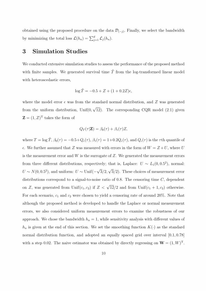
3 Simulation Studies
We conducted extensive simulation studies to assess the performance of the proposed method
with finite samples. We generated survival time T from the log-transformed linear model
with heteroscedastic errors,
log T = −0.5 + Z + (1 + 0.2Z)ε,
where the model error ε was from the standard normal distribution, and Z was generated
from the uniform distribution, Unif(0,√
12). The corresponding CQR model (2.1) given
Z = (1, Z)T takes the form of
QT (τ |Z) = β0(τ) + β1(τ)Z,
where T = log T , β0(τ) = −0.5+Qε(τ), β1(τ) = 1+0.2Qε(τ), and Qε(τ) is the τth quantile of
ε. We further assumed that Z was measured with errors in the form of W = Z +U , where U
is the measurement error and W is the surrogate of Z. We generated the measurement errors
from three different distributions, respectively; that is, Laplace: U ∼ L1(0, 0.52), normal:
U ∼ N(0, 0.52), and uniform: U ∼ Unif(−√3/2,√
3/2). These choices of measurement error
distributions correspond to a signal-to-noise ratio of 0.8. The censoring time C, dependent
on Z, was generated from Unif(c1, c2) if Z <√
12/2 and from Unif(c1 + 1, c2) otherwise.
For each scenario, c1 and c2 were chosen to yield a censoring rate of around 20%. Note that
although the proposed method is developed to handle the Laplace or normal measurement
errors, we also considered uniform measurement errors to examine the robustness of our
approach. We chose the bandwidth hn = 1, while sensitivity analysis with different values of
hn is given at the end of this section. We set the smoothing function K(·) as the standard
normal distribution function, and adopted an equally spaced grid over interval [0.1, 0.78]
with a step 0.02. The naive estimator was obtained by directly regressing on W = (1,W )T.
10
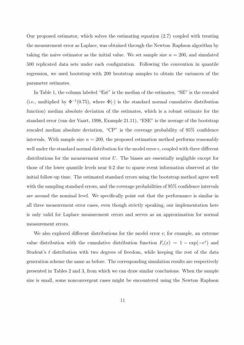
Our proposed estimator, which solves the estimating equation (2.7) coupled with treating
the measurement error as Laplace, was obtained through the Newton–Raphson algorithm by
taking the naive estimator as the initial value. We set sample size n = 200, and simulated
500 replicated data sets under each configuration. Following the convention in quantile
regression, we used bootstrap with 200 bootstrap samples to obtain the variances of the
parameter estimates.
In Table 1, the column labeled “Est” is the median of the estimates, “SE” is the rescaled
(i.e., multiplied by Φ−1(0.75), where Φ(·) is the standard normal cumulative distribution
function) median absolute deviation of the estimates, which is a robust estimate for the
standard error (van der Vaart, 1998, Example 21.11), “ESE” is the average of the bootstrap
rescaled median absolute deviation, “CP” is the coverage probability of 95% confidence
intervals. With sample size n = 200, the proposed estimation method performs reasonably
well under the standard normal distribution for the model error ε, coupled with three different
distributions for the measurement error U . The biases are essentially negligible except for
those of the lower quantile levels near 0.2 due to sparse event information observed at the
initial follow-up time. The estimated standard errors using the bootstrap method agree well
with the sampling standard errors, and the coverage probabilities of 95% confidence intervals
are around the nominal level. We specifically point out that the performance is similar in
all three measurement error cases, even though strictly speaking, our implementation here
is only valid for Laplace measurement errors and serves as an approximation for normal
measurement errors.
We also explored different distributions for the model error ε; for example, an extreme
value distribution with the cumulative distribution function Fε(x) = 1 − exp(−ex) and
Student’s t distribution with two degrees of freedom, while keeping the rest of the data
generation scheme the same as before. The corresponding simulation results are respectively
presented in Tables 2 and 3, from which we can draw similar conclusions. When the sample
size is small, some nonconvergent cases might be encountered using the Newton–Raphson
11
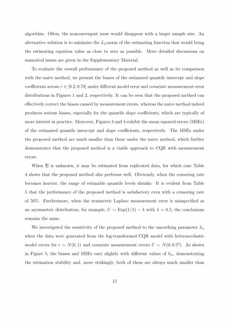
algorithm. Often, the nonconvergent issue would disappear with a larger sample size. An
alternative solution is to minimize the L2-norm of the estimating function that would bring
the estimating equation value as close to zero as possible. More detailed discussions on
numerical issues are given in the Supplementary Material.
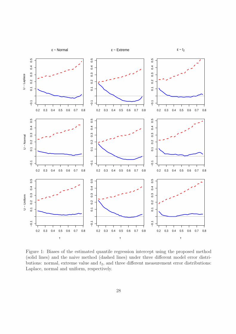
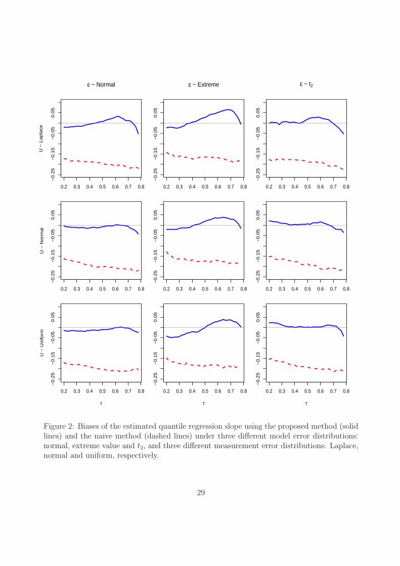
To evaluate the overall performance of the proposed method as well as its comparison
with the naive method, we present the biases of the estimated quantile intercept and slope
coefficients across τ ∈ [0.2, 0.78] under different model error and covariate measurement error
distributions in Figures 1 and 2, respectively. It can be seen that the proposed method can
effectively correct the biases caused by measurement errors, whereas the naive method indeed
produces serious biases, especially for the quantile slope coefficients, which are typically of
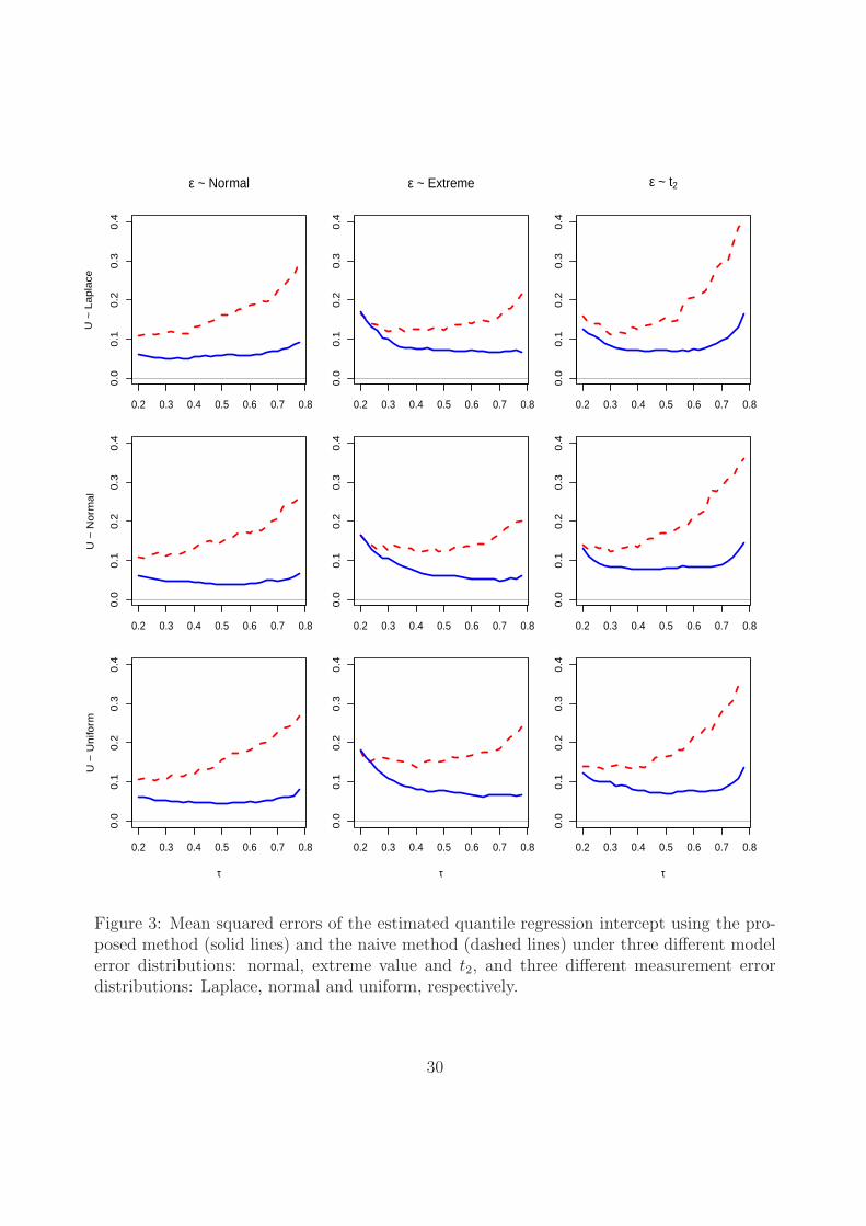
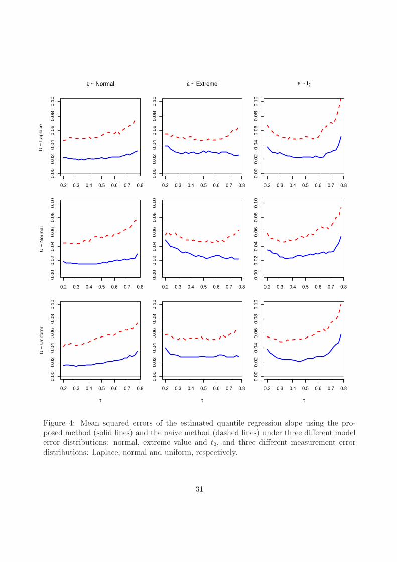
more interest in practice. Moreover, Figures 3 and 4 exhibit the mean squared errors (MSEs)
of the estimated quantile intercept and slope coefficients, respectively. The MSEs under
the proposed method are much smaller than those under the naive method, which further
demonstrates that the proposed method is a viable approach to CQR with measurement
errors.
When Σ is unknown, it may be estimated from replicated data, for which case Table
4 shows that the proposed method also performs well. Obviously, when the censoring rate
becomes heavier, the range of estimable quantile levels shrinks. It is evident from Table
5 that the performance of the proposed method is satisfactory even with a censoring rate
of 50%. Furthermore, when the symmetric Laplace measurement error is misspecified as
an asymmetric distribution, for example, U ∼ Exp(1/λ) − λ with λ = 0.5, the conclusions
remains the same.
We investigated the sensitivity of the proposed method to the smoothing parameter hn
when the data were generated from the log-transformed CQR model with heteroscedastic
model errors for ε ∼ N(0, 1) and covariate measurement errors U ∼ N(0, 0.52). As shown
in Figure 5, the biases and MSEs vary slightly with different values of hn, demonstrating
the estimation stability and, more strikingly, both of them are always much smaller than
12

those from the naive method. We also explored the situation where multiple covariates are
subject to measurement errors while others are measured precisely. For normal measurement
errors, we conducted simulations to compare our infinite series correction function with the
integral correction function proposed by Wang, Stefanski, and Zhu (2012). In addition, we
examined the simulation and extrapolation (SIMEX) method in He, Yi, and Xiong (2007)
under the AFT model, and the simulation results in the Supplemental Material demonstrate
the comparability of our proposed method with other alternatives.
4 Application
As an illustration, we applied the proposed estimation and inference procedure for CQR
with measurement errors to a lung cancer study. This data set contains 280 lung cancer
patients, whose survival times were recorded with a censoring rate of 64.3%. One of the
main objectives of this study was to assess the association of patient survival with certain
biomarker expression in the tumor cell cytoplasm. The reading of the biomarker expression
was performed by pathologists and could be subjective. As a result, the readings of the
biomarker expression for each patient were considered imprecise measurements. To reduce
the possible subjectivity of the evaluation, for some patients, two readings of the biomarker
expression were provided by two different pathologists (replicates). However, neither of the
two measurements of biomarker expression can be considered precise. Our main interest lies
in investigating the potential of the biomarker as a new prognostic marker and therapeutic
target for lung cancer. Other confounding covariates of interest include tumor histology
(there were 61% of patients with adenocarcinoma coded as 1, and 39% squamous cell car-
cinoma coded as 0), age (ranging from 34 to 90 years with mean 66 years), and sex (52%
female coded as 1, 48% male coded as 0). In our analysis, we standardized the patients’ ages
by subtracting their mean and dividing their standard deviation. Half of the patients in the
data set had duplicated readings of the biomarker expression and the averaged value of the
two expression readings was considered as the surrogate variable in our analysis. Based on
13
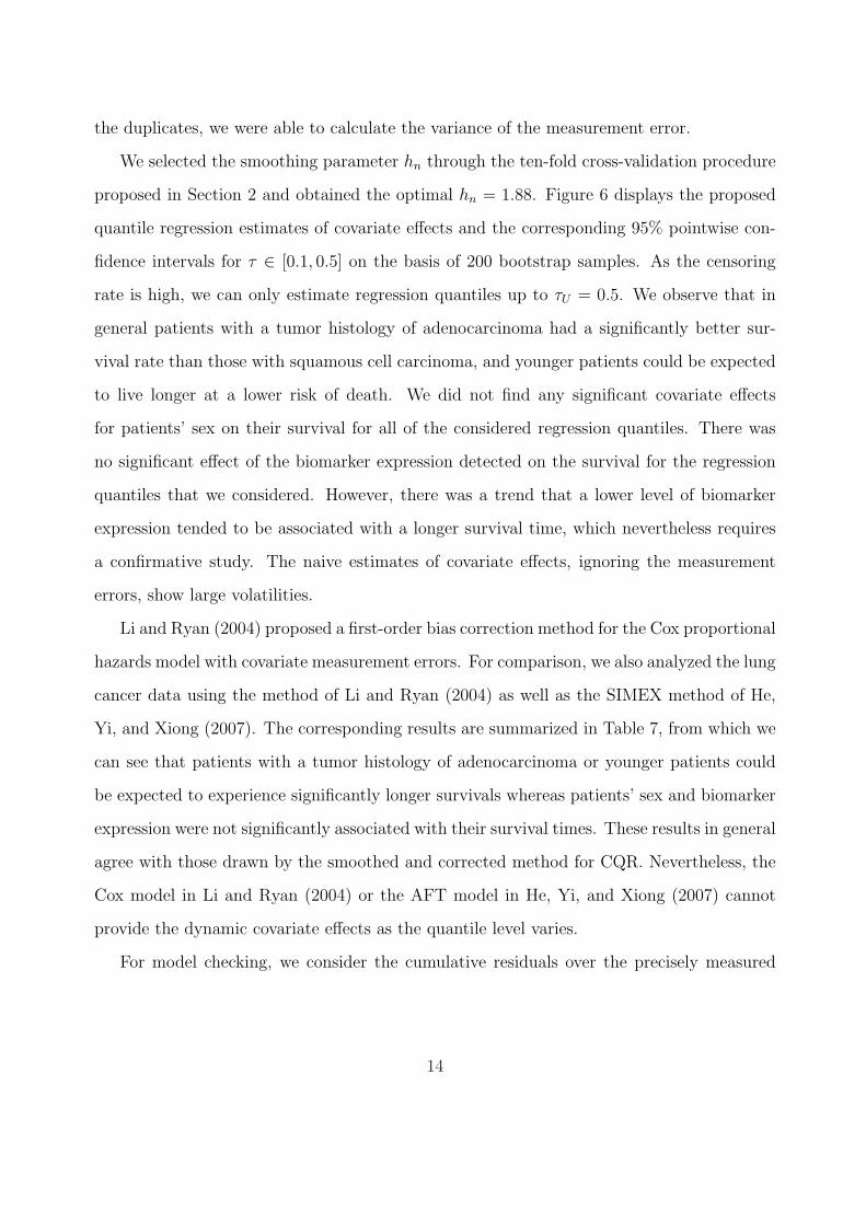
the duplicates, we were able to calculate the variance of the measurement error.
We selected the smoothing parameter hn through the ten-fold cross-validation procedure
proposed in Section 2 and obtained the optimal hn = 1.88. Figure 6 displays the proposed
quantile regression estimates of covariate effects and the corresponding 95% pointwise con-
fidence intervals for τ ∈ [0.1, 0.5] on the basis of 200 bootstrap samples. As the censoring
rate is high, we can only estimate regression quantiles up to τU = 0.5. We observe that in
general patients with a tumor histology of adenocarcinoma had a significantly better sur-
vival rate than those with squamous cell carcinoma, and younger patients could be expected
to live longer at a lower risk of death. We did not find any significant covariate effects
for patients’ sex on their survival for all of the considered regression quantiles. There was
no significant effect of the biomarker expression detected on the survival for the regression
quantiles that we considered. However, there was a trend that a lower level of biomarker
expression tended to be associated with a longer survival time, which nevertheless requires
a confirmative study. The naive estimates of covariate effects, ignoring the measurement
errors, show large volatilities.
Li and Ryan (2004) proposed a first-order bias correction method for the Cox proportional
hazards model with covariate measurement errors. For comparison, we also analyzed the lung
cancer data using the method of Li and Ryan (2004) as well as the SIMEX method of He,
Yi, and Xiong (2007). The corresponding results are summarized in Table 7, from which we
can see that patients with a tumor histology of adenocarcinoma or younger patients could
be expected to experience significantly longer survivals whereas patients’ sex and biomarker
expression were not significantly associated with their survival times. These results in general
agree with those drawn by the smoothed and corrected method for CQR. Nevertheless, the
Cox model in Li and Ryan (2004) or the AFT model in He, Yi, and Xiong (2007) cannot
provide the dynamic covariate effects as the quantile level varies.
For model checking, we consider the cumulative residuals over the precisely measured
14
covariates,
T (wo, τ) = n−1/2
n∑i=1
I(Woi ≤ wo)M(Oi, βn(τ); hn).
where Wo = (Histology, Age, Sex)T represent the error-free covariates excluding the biomarker
expression. The null distribution of T (wo, τ) can be approximated by the zero-mean process
T ∗(wo, τ) = n−1/2
n∑i=1
I(Woi ≤ wo)M(Oi, βn(τ); hn)Gi,
where (G1, . . . , Gn) were generated independently from the standard normal distribution
while fixing the data {(Xi, ∆i,Wi), i = 1, . . . , n} at their observed values. The supremum
statistic supwo,τ |T (wo, τ)| can be used to test the overall fit of the CQR model. We gener-
ated a large number of, say 1000, realizations from supwo,τ |T ∗(wo, τ)| and obtained its 95th
percentile as 1.827. The observed value of supwo,τ |T (wo, τ)| is 0.394, which indicates that
the global linear CQR model fits the lung cancer data well.
5 Remarks
We have proposed a corrected estimating equation approach to CQR models for survival
data when covariates are measured with errors. Using a smooth function to approximate
the indicator function, the resultant estimating function is smoothed, and thus conventional
iterative root-finding procedures, such as the Newton–Raphson algorithm, can be applied
(Wang, Stefanski, and Zhu, 2012). We have established the asymptotic consistency and
weak convergence of the proposed estimator through modern empirical process techniques.
Numerical results show that the proposed method is promising in terms of correcting the
bias arising from covariate measurement errors, whereas the naive method typically produces
biased estimates.
For variance estimation, we also explored directly using the sandwich-type variance esti-
mator based on the smoothed estimating equation (2.6), but the resulting coverage probabil-
ity is found to be generally over the nominal level. A more interesting resampling method,
known as the Markov chain marginal bootstrap, can be tailored for variance estimation in
15

quantile regression (Kocherginsky, He, and Mu, 2005). When the covariates are of high
dimension, particularly for those mismeasured ones, estimation could be difficult, whereas
some regularization methods may potentially be incorporated into the estimation procedure
to alleviate the instability caused by high dimensionality.
Identifiability is an inherent and subtle issue in CQR. Regression quantiles with τ close
to 1 may not be identifiable due to the lack of event information in the upper tail. Theoret-
ically, τU should satisfy the identifiability Assumption 4-(iii) in the Appendix. In practical
implementation, we first set τU to be close to one minus the censoring rate, and then select
the final τU in an adaptive manner as follows. If all the regression quantiles over [ν, τU ] can
be estimated, we increase τU by some small step size, e.g., 0.05 or 0.1; otherwise, we decrease
τU slightly. Through this trial-and-error process, we can push τU to the largest value at
which the model parameters can be identified. Similarly, ν could also be chosen in such an
adaptive way.
The proposed method requires the global linearity assumption as in Portnoy (2003),
Peng and Huang (2008) and Wei and Carroll (2009); that is, in order to estimate the τth
conditional regression quantile, it is necessary to assume that the conditional functionals at
all the lower quantiles are also in the linear form. When the linearity assumption holds only
at one specific quantile level τ of interest, research along the work of Wang and Wang (2009)
is warranted.
Appendix: Assumptions
Let ‖·‖ denote the L2-norm of the corresponding vector or matrix after vectorization. Define
r0 = inf{j ≥ 1:∫∞−∞ xjK(1)(x)dx 6= 0}. Let SC(t|z) = P (C > t|z), FX,∆=1(t|z) = P (X ≤
t, ∆ = 1|z) and FX(t|z) = P (X ≤ t|z), and then FX,∆=1(t|z) =∫ t
−∞ SC(u|z)dFT (u|z) and
FX(t|z) = 1 − {1 − FT (t|z)}SC(t|z). Further denote µ0(b) = E{ZN(ZTb)}, µ(b; hn) =
E{∆g(O,b; hn)}, µ0(b) = E{ZI(X ≥ ZTb)}, and µ(b; hn) = E{g(O,b; hn)}.
16

For d > 0, define B(d) = {b ∈ Rp: infτ∈(0,τU ] ‖µ0(b) − µ0{β0(τ)}‖ ≤ d}. Assume
that there exists d0 > 0 such that B(d0) contains {β0(τ): τ ∈ (0, τU ]}. Denote fX,∆=1(t|z)and fX(t|z) as the density functions corresponding to FX,∆=1(t|z) and FX(t|z), respectively.
Let B0(b) = E{ZZTfX,∆=1(ZTb|Z)} and J0(b) = −E{ZZTfX(ZTb|Z)}. Finally, denote
g{O,β(τ); hn} = ∂g{O,β(τ); hn}/∂β(τ).
Assumption 1. The smoothing function K(·) satisfies:
(i) K(j)(·) is uniformly bounded for j = 0, . . . , 4 in the Laplace measurement error
model and for j ≥ 0 in the normal measurement error model.
(ii) r0 ≥ 2 and for each integer j (0 ≤ j ≤ r0),∫∞−∞ |xjK(1)(x)|dx < ∞.
(iii) For each integer j (0 ≤ j ≤ r0), any η > 0, and any sequence hn converging to 0,
limn→∞ hj−r0n
∫|hnx|>η
|xjK(1)(x)|dx = 0 and limn→∞ h−1n
∫|hnx|>η
|K(2)(x)|dx = 0.
Assumption 2. For each integer j such that 1 ≤ j ≤ r0, F(j)T (t|z) is a continuous function
of z and uniformly bounded over t and z, where F(j)T (t|z) is the jth derivative of FT (t|z)
with respect to t. So is S(j)C (t|z).
Assumption 3. Each component of µ0{β(τ)}, µ{β(τ); hn}, µ0{β(τ)}, and µ{β(τ); hn}as a function of τ is Lipschitz continuous.
Assumption 4. Boundedness conditions are imposed:
(i) Both E(‖Z‖2) and E(‖U‖2) are bounded, and E(ZZT) is positive definite.
(ii) fX,∆=1(ZTb|Z) is bounded away from zero for all b in B(d0).
(iii) infτ∈[ν,τU ] eigmin[B0{β0(τ)}] > 0 for any 0 < ν ≤ τU , where eigmin(·) denotes the
minimum eigenvalue of a matrix.
(iv) The norm of J0(b)B0(b)−1 is uniformly bounded for all b in B(d0).
Assumption 5. We assume that
17

(i) supτ∈[ν,τU ] ‖E[g{O,β0(τ); hn}]2‖ is bounded as n →∞ for any ν ∈ (0, τU ].
(ii) E[g{O, β(τ); hn}]2 is component-wise continuous in sup-norm as a functional of
β(τ).
Assumption 1 holds if K(·) is the standard normal cumulative distribution function.
Apparently, FX,∆=1(t|z) and FX(t|z) satisfy a similar boundedness condition as Assumption
2, which is a standard assumption in survival analysis. Assumptions 3 and 4 are commonly
used in CQR models (Peng and Huang, 2009). Assumption 5 essentially imposes a higher
convergence rate of the smoothing parameter hn compared with Assumption 1-(iii). If we
take K(·) to be the standard normal cumulative distribution function, Assumption 5 holds for
both the Laplace and the normal measurement errors. This is because the exponential part
can be factored out for any order of derivatives with respect to K(·) and the component-wise
continuity follows directly.
References
Bang, H., and Tsiatis, A. A. (2002), “Median Regression With Censored Cost Data,”
Biometrics, 58, 643–649.
Brown, M. L. (1982), “Robust Line Estimation With Error in Both Variables,” Journal of
the American Statistical Association, 77, 71–79. Correction in 78, 1008.
Buchinsky, M., and Hahn, J. Y. (1998), “An Alternative Estimator for Censored Quantile
Regression,” Econometrica, 66, 653–671.
Buckley, J., and James, I. (1979), “Linear Regression With Censored Data,” Biometrika,
66, 429–436.
Carroll, R. J., Ruppert, D., Stefanski, L. A., and Crainiceanu, C. (2006), Measurement
Error in Nonlinear Models: A Modern Perspective, London: CRC Press.
18

Chernozhukov, V., and Hong, H. (2002), “Three-Step Censored Quantile Regression and
Extramarital Affairs,” Journal of the American Statistical Association, 97, 872–882.
Cox, D. R. (1972), “Regression Models and Life Tables” (with discussion), Journal of Royal
Statistical Society, Ser. B, 34, 187–220.
Fitzenberger, B. (1997), “A Guide to Censored Quantile Regressions,” in Handbook of
Statistics, Robust Inference, eds. Maddala G. S., and Rao C. R., Amsterdam: North-
Holland.
Fleming, T. R., and Harrington, D. (1991), Counting Processes and Survival Analysis, New
York: Wiley.
He, X., and Liang, H. (2000), “Quantile Regression Estimates for a Class of Linear and
Partially Linear Errors-in-Variables Models,” Statistica Sinica, 10, 129–140.
He, W., Yi, G. Y., and Xiong, J. (2007), “Accelerated Failure Time Models With Covariates
Subject to Measurement Error,” Statistics in Medicine, 26, 4817–4832.
Hong, H., and Tamer, E. (2003), “A Simple Estimator for Nonlinear Error in Variable
Models,” Journal of Econometrics, 117, 1–19.
Horowitz, J. (1992), “A Smoothed Maximum Score Estimator for the Binary Response
Model,” Econometrica, 60, 505–531.
Horowitz, J. (1998), “Bootstrap Methods for Median Regression Model,” Econometrica, 66,
1327–1352.
Jin, Z., Lin, D. Y., Wei, L. J., and Ying, Z. (2003), “Rank-Based Inference for the Accel-
erated Failure Time Model,” Biometrika, 90, 341–353.
Khan, S., and Powell, L. J. (2001), “Two-Step Estimation of Semiparametric Censored
Regression Models,” Journal of Econometrics, 103, 73–110.
19

Kocherginsky, M., He, X., and Mu, Y. (2005), “Practical Confidence Intervals for Regression
Quantiles,” Journal of Computational and Graphical Statistics, 14, 41–55.
Koenker, R. (2005), Quantile Regression, New York: Cambridge University Press.
Koenker, R., and Bassett, G. J. (1978), “Regression Quantiles,” Econometrica, 46, 33–50.
Koenker, R., and Geling, O. (2001), “Reappraising Medfly Longevity: A Quantile Regres-
sion Survival Analysis,” Journal of the American Statistical Association, 96, 458–468.
Kotz, S., Kozubowski, T. J., and Podgorski, K. (2001), The Laplace Distribution and Gen-
eralizations, New York: Springer.
Lai, T. L., and Ying, Z. (1991), “Rank Regression Methods for Left-Truncated and Right-
Censored Data,” The Annals of Statistics, 19, 531–556.
Li, Y., and Ryan, L. (2004), “Survival Analysis With Heterogeneous Covariate Measurement
Error,” Journal of the American Statistical Association, 99, 724–735.
Lindgren, A. (1997), “Quantile Regression With Censored Data Using Generalized L1 Min-
imization,” Computational Statistics and Data Analysis, 23, 509–524.
Ma, Y., and Yin, G. (2011), “Censored Quantile Regression With Covariate Measurement
Errors,” Statistica Sinica, 21, 949–971.
Nakamura, T. (1990), “Corrected Score Function for Errors-in-Variables Models: Method-
ology and Application to Generalized Linear Models,” Biometrika, 77, 127–137.
Peng, L., and Huang, Y. (2008), “Survival Analysis With Quantile Regression Models,”
Journal of the American Statistical Association, 103, 637–649.
Portnoy, S. (2003), “Censored Regression Quantiles,” Journal of the American Statistical
Association, 98, 1001–1012.
20
Powell, J. L. (1984), “Least Absolute Deviations Estimation for the Censored Regression,”
Journal of Econometrics, 25, 303–325.
Prentice, R. L. (1978), “Linear Rank Tests With Right Censored Data,” Biometrika, 65,
167–180.
Ritov, Y. (1990), “Estimation in a Linear Regression Model With Censored Data,” The
Annals of Statistics, 18, 303–328.
Stefanski, L. A. (1989), “Unbiased Estimation of a Nonlinear Function of a Normal-Mean
With Application to Measurement Error Models,” Communications in Statistics-Theory
and Methods, 18, 4335–4358.
Tsiatis, A. A. (1990), “Estimating Regression Parameters Using Linear Rank Tests for
Censored Data,” The Annals of Statistics, 18, 354–372.
van der Vaart, A. W. (1998), Asymptotic Statistics, New York: Cambridge University Press.
Wang, H., and Wang, L. (2009), “Locally Weighted Censored Quantile Regression,” Journal
of the American Statistical Association, 104, 1117–1128.
Wang, H., Stefanski, L. A., and Zhu, Z. (2012), “Corrected-Loss Estimation for Quantile
Regression With Covariate Measurement Errors,” Biometrika, 99, 405–421.
Wei, L. J., Ying, Z., and Lin, D. Y. (1990), “Linear Regression Analysis of Censored Survival
Data Based on Rank Tests,” Biometrika, 77, 845–851.
Wei, Y., and Carroll, R. J. (2009), “Quantile Regression With Measurement Error,” Journal
of the American Statistical Association, 104, 1129–1143.
Yang, S. (1999), “Censored Median Regression Using Weighted Empirical Survival and
Hazard Function,” Journal of the American Statistical Association, 94, 137–145.
21

Ying, Z., Jung, S. H., and Wei, L. J. (1995), “Survival Analysis With Median Regression
Models,” Journal of the American Statistical Association, 90, 178–184.
22

Table 1: Simulation results for the log-transformed censored quantile regression with threedifferent distributions of covariate measurement errors and heteroscedastic model errors forε ∼ N(0, 1)
β0(·) β1(·)τ True Est SE/ESE CP(%) True Est SE/ESE CP(%)
U ∼ L1(0, 0.52)
0.2 −1.342 −1.245 0.934 91.8 0.832 0.811 1.028 93.40.3 −1.024 −0.976 0.953 94.0 0.895 0.881 1.014 92.80.4 −0.753 −0.740 1.022 95.6 0.949 0.944 1.021 94.20.5 −0.500 −0.509 1.030 95.8 1.000 1.006 1.028 93.20.6 −0.247 −0.269 0.996 95.6 1.051 1.080 0.974 93.40.7 0.024 −0.001 1.040 95.0 1.105 1.117 1.038 93.2
U ∼ N(0, 0.52)0.2 −1.342 −1.265 0.967 92.8 0.832 0.830 0.993 94.00.3 −1.024 −0.975 0.943 92.0 0.895 0.885 0.932 93.60.4 −0.753 −0.715 0.928 93.8 0.949 0.936 0.925 93.80.5 −0.500 −0.465 0.879 93.0 1.000 0.993 0.935 94.20.6 −0.247 −0.222 0.886 94.2 1.051 1.053 0.972 93.60.7 0.024 0.044 0.913 94.6 1.105 1.099 0.942 92.8
U ∼ Unif(−√3/2,√
3/2)0.2 −1.342 −1.260 0.987 92.6 0.832 0.817 0.891 94.80.3 −1.024 −0.971 0.969 93.6 0.895 0.878 0.894 94.80.4 −0.753 −0.720 0.951 93.8 0.949 0.934 0.962 92.80.5 −0.500 −0.476 0.942 94.2 1.000 0.990 0.986 92.60.6 −0.247 −0.222 0.969 93.8 1.051 1.050 1.042 93.60.7 0.024 0.060 1.004 94.2 1.105 1.102 1.052 92.6
Note: SE/ESE is the ratio of the sampling standard error and the estimated (bootstrap) standard error, andCP is the coverage probability.
23

Table 2: Simulation results for the log-transformed censored quantile regression with threedifferent distributions of covariate measurement errors and heteroscedastic model errors forε from an extreme value distribution
β0(·) β1(·)τ True Est SE/ESE CP(%) True Est SE/ESE CP(%)
U ∼ L1(0, 0.52)
0.2 −2.000 −1.822 1.030 85.4 0.700 0.679 0.929 93.40.3 −1.531 −1.452 1.000 90.8 0.794 0.770 0.934 93.40.4 −1.172 −1.161 0.965 92.4 0.866 0.870 0.994 93.20.5 −0.867 −0.918 0.993 92.2 0.927 0.954 1.030 92.40.6 −0.587 −0.666 1.008 91.2 0.983 1.033 0.994 90.20.7 −0.314 −0.384 0.996 91.8 1.037 1.100 0.981 92.4
U ∼ N(0, 0.52)0.2 −2.000 −1.823 1.008 85.6 0.700 0.680 1.042 94.00.3 −1.531 −1.453 1.026 91.0 0.794 0.778 1.050 94.40.4 −1.172 −1.154 0.957 93.8 0.866 0.863 1.018 94.60.5 −0.867 −0.895 0.950 94.2 0.927 0.946 0.957 94.60.6 −0.587 −0.635 0.923 93.2 0.983 1.018 1.013 93.00.7 −0.314 −0.349 0.876 95.2 1.037 1.066 0.974 94.8
U ∼ Unif(−√3/2,√
3/2)0.2 −2.000 −1.771 1.008 85.4 0.700 0.657 0.933 94.40.3 −1.531 −1.418 1.023 90.4 0.794 0.749 0.911 94.80.4 −1.172 −1.119 1.018 91.6 0.866 0.847 0.959 93.80.5 −0.867 −0.854 1.073 93.2 0.927 0.926 1.031 92.80.6 −0.587 −0.601 1.061 92.2 0.983 1.012 1.051 91.80.7 −0.314 −0.314 1.080 91.8 1.037 1.073 1.032 91.8
24

Table 3: Simulation results for the log-transformed censored quantile regression with threedifferent distributions of covariate measurement errors and heteroscedastic model errors forε ∼ t2
β0(·) β1(·)τ True Est SE/ESE CP(%) True Est SE/ESE CP(%)
U ∼ L1(0, 0.52)
0.2 −1.561 −1.453 0.974 90.6 0.788 0.788 0.923 96.60.3 −1.117 −1.101 0.973 95.8 0.877 0.881 0.960 95.80.4 −0.789 −0.797 0.978 96.0 0.942 0.947 0.916 96.40.5 −0.500 −0.512 0.960 96.0 1.000 1.020 0.898 95.20.6 −0.211 −0.223 0.955 94.2 1.058 1.085 0.872 93.80.7 0.117 0.116 0.991 95.0 1.123 1.122 0.920 93.8
U ∼ N(0, 0.52)0.2 −1.561 −1.452 0.975 92.0 0.788 0.810 0.908 95.00.3 −1.117 −1.082 0.973 95.0 0.877 0.885 0.935 94.60.4 −0.789 −0.763 1.026 95.2 0.942 0.947 0.981 95.80.5 −0.500 −0.477 1.041 95.0 1.000 1.006 1.025 94.60.6 −0.211 −0.193 1.036 95.0 1.058 1.073 1.030 94.80.7 0.117 0.161 0.967 94.8 1.123 1.114 0.967 93.6
U ∼ Unif(−√3/2,√
3/2)0.2 −1.561 −1.490 0.937 90.6 0.788 0.810 0.920 94.20.3 −1.117 −1.109 1.050 93.2 0.877 0.889 0.918 93.20.4 −0.789 −0.789 1.026 93.0 0.942 0.943 0.962 93.80.5 −0.500 −0.478 0.985 93.4 1.000 1.001 0.981 93.00.6 −0.211 −0.179 1.004 93.4 1.058 1.059 1.018 92.60.7 0.117 0.156 0.946 92.0 1.123 1.131 1.033 91.4
25
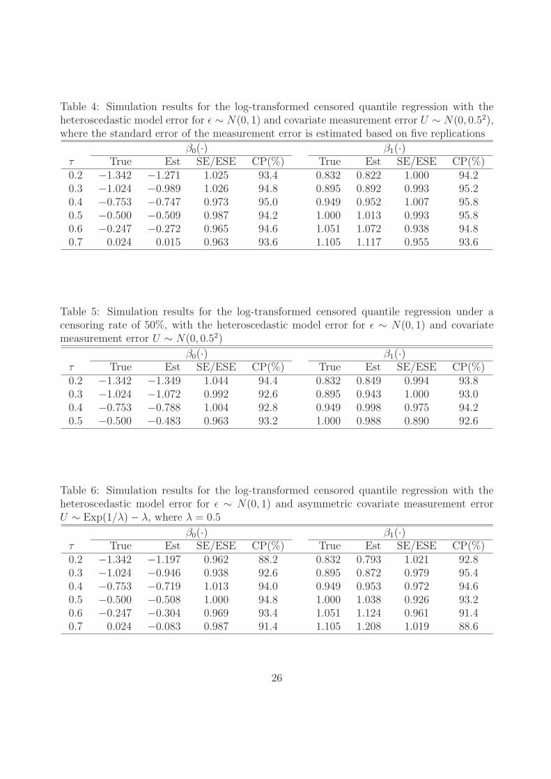
Table 4: Simulation results for the log-transformed censored quantile regression with theheteroscedastic model error for ε ∼ N(0, 1) and covariate measurement error U ∼ N(0, 0.52),where the standard error of the measurement error is estimated based on five replications
β0(·) β1(·)τ True Est SE/ESE CP(%) True Est SE/ESE CP(%)0.2 −1.342 −1.271 1.025 93.4 0.832 0.822 1.000 94.20.3 −1.024 −0.989 1.026 94.8 0.895 0.892 0.993 95.20.4 −0.753 −0.747 0.973 95.0 0.949 0.952 1.007 95.80.5 −0.500 −0.509 0.987 94.2 1.000 1.013 0.993 95.80.6 −0.247 −0.272 0.965 94.6 1.051 1.072 0.938 94.80.7 0.024 0.015 0.963 93.6 1.105 1.117 0.955 93.6
Table 5: Simulation results for the log-transformed censored quantile regression under acensoring rate of 50%, with the heteroscedastic model error for ε ∼ N(0, 1) and covariatemeasurement error U ∼ N(0, 0.52)
β0(·) β1(·)τ True Est SE/ESE CP(%) True Est SE/ESE CP(%)0.2 −1.342 −1.349 1.044 94.4 0.832 0.849 0.994 93.80.3 −1.024 −1.072 0.992 92.6 0.895 0.943 1.000 93.00.4 −0.753 −0.788 1.004 92.8 0.949 0.998 0.975 94.20.5 −0.500 −0.483 0.963 93.2 1.000 0.988 0.890 92.6
Table 6: Simulation results for the log-transformed censored quantile regression with theheteroscedastic model error for ε ∼ N(0, 1) and asymmetric covariate measurement errorU ∼ Exp(1/λ)− λ, where λ = 0.5
β0(·) β1(·)τ True Est SE/ESE CP(%) True Est SE/ESE CP(%)0.2 −1.342 −1.197 0.962 88.2 0.832 0.793 1.021 92.80.3 −1.024 −0.946 0.938 92.6 0.895 0.872 0.979 95.40.4 −0.753 −0.719 1.013 94.0 0.949 0.953 0.972 94.60.5 −0.500 −0.508 1.000 94.8 1.000 1.038 0.926 93.20.6 −0.247 −0.304 0.969 93.4 1.051 1.124 0.961 91.40.7 0.024 −0.083 0.987 91.4 1.105 1.208 1.019 88.6
26

Table 7: Analysis results of the lung cancer data using the first-order bias correction methodfor the Cox proportional hazards model (Li and Ryan, 2004) and the simulation-extrapolationmethod for the accelerated failure time (AFT) model (He, Yi, and Xiong, 2007)
Model Error Covariate Est ESE p-valueCox – Histology −0.503 0.219 0.022
Age 0.433 0.118 < 0.001Sex −0.081 0.209 0.699Biomarker 0.043 0.183 0.813
AFT Normal Intercept 1.275 0.614 0.038Histology 0.680 0.325 0.036Age −0.500 0.159 0.002Sex 0.210 0.303 0.487Biomarker 0.178 0.300 0.552
Extreme Intercept 2.108 0.501 < 0.001Histology 0.569 0.262 0.030Age −0.490 0.131 < 0.001Sex 0.100 0.238 0.673Biomarker −0.070 0.246 0.776
27
ε ~ Normal
U ~
La
pla
ce
0.2 0.3 0.4 0.5 0.6 0.7 0.8
−0
.10
.10
.20
.30
.40
.5
U ~
No
rma
l
0.2 0.3 0.4 0.5 0.6 0.7 0.8
−0
.10
.10
.20
.30
.40
.5
τ
U ~
Un
iform
0.2 0.3 0.4 0.5 0.6 0.7 0.8
−0
.10
.10
.20
.30
.40
.5
ε ~ Extreme
0.2 0.3 0.4 0.5 0.6 0.7 0.8
−0
.10
.10
.20
.30
.40
.5
0.2 0.3 0.4 0.5 0.6 0.7 0.8
−0
.10
.10
.20
.30
.40
.5
τ
0.2 0.3 0.4 0.5 0.6 0.7 0.8
−0
.10
.10
.20
.30
.40
.5
ε ~ t2
0.2 0.3 0.4 0.5 0.6 0.7 0.8
−0
.10
.10
.20
.30
.40
.5
0.2 0.3 0.4 0.5 0.6 0.7 0.8
−0
.10
.10
.20
.30
.40
.5
τ
0.2 0.3 0.4 0.5 0.6 0.7 0.8
−0
.10
.10
.20
.30
.40
.5
Figure 1: Biases of the estimated quantile regression intercept using the proposed method(solid lines) and the naive method (dashed lines) under three different model error distri-butions: normal, extreme value and t2, and three different measurement error distributions:Laplace, normal and uniform, respectively.
28
ε ~ Normal
U ~
La
pla
ce
0.2 0.3 0.4 0.5 0.6 0.7 0.8
−0
.25
−0
.15
−0
.05
0.0
5
U ~
No
rma
l
0.2 0.3 0.4 0.5 0.6 0.7 0.8
−0
.25
−0
.15
−0
.05
0.0
5
τ
U ~
Un
iform
0.2 0.3 0.4 0.5 0.6 0.7 0.8
−0
.25
−0
.15
−0
.05
0.0
5
ε ~ Extreme
0.2 0.3 0.4 0.5 0.6 0.7 0.8
−0
.25
−0
.15
−0
.05
0.0
5
0.2 0.3 0.4 0.5 0.6 0.7 0.8
−0
.25
−0
.15
−0
.05
0.0
5
τ
0.2 0.3 0.4 0.5 0.6 0.7 0.8
−0
.25
−0
.15
−0
.05
0.0
5
ε ~ t2
0.2 0.3 0.4 0.5 0.6 0.7 0.8
−0
.25
−0
.15
−0
.05
0.0
5
0.2 0.3 0.4 0.5 0.6 0.7 0.8
−0
.25
−0
.15
−0
.05
0.0
5
τ
0.2 0.3 0.4 0.5 0.6 0.7 0.8
−0
.25
−0
.15
−0
.05
0.0
5
Figure 2: Biases of the estimated quantile regression slope using the proposed method (solidlines) and the naive method (dashed lines) under three different model error distributions:normal, extreme value and t2, and three different measurement error distributions: Laplace,normal and uniform, respectively.
29
ε ~ Normal
U ~
La
pla
ce
0.2 0.3 0.4 0.5 0.6 0.7 0.8
0.0
0.1
0.2
0.3
0.4
U ~
No
rma
l
0.2 0.3 0.4 0.5 0.6 0.7 0.8
0.0
0.1
0.2
0.3
0.4
τ
U ~
Un
iform
0.2 0.3 0.4 0.5 0.6 0.7 0.8
0.0
0.1
0.2
0.3
0.4
ε ~ Extreme
0.2 0.3 0.4 0.5 0.6 0.7 0.8
0.0
0.1
0.2
0.3
0.4
0.2 0.3 0.4 0.5 0.6 0.7 0.8
0.0
0.1
0.2
0.3
0.4
τ
0.2 0.3 0.4 0.5 0.6 0.7 0.8
0.0
0.1
0.2
0.3
0.4
ε ~ t2
0.2 0.3 0.4 0.5 0.6 0.7 0.8
0.0
0.1
0.2
0.3
0.4
0.2 0.3 0.4 0.5 0.6 0.7 0.8
0.0
0.1
0.2
0.3
0.4
τ
0.2 0.3 0.4 0.5 0.6 0.7 0.8
0.0
0.1
0.2
0.3
0.4
Figure 3: Mean squared errors of the estimated quantile regression intercept using the pro-posed method (solid lines) and the naive method (dashed lines) under three different modelerror distributions: normal, extreme value and t2, and three different measurement errordistributions: Laplace, normal and uniform, respectively.
30
ε ~ Normal
U ~
La
pla
ce
0.2 0.3 0.4 0.5 0.6 0.7 0.8
0.0
00
.02
0.0
40
.06
0.0
80
.10
U ~
No
rma
l
0.2 0.3 0.4 0.5 0.6 0.7 0.8
0.0
00
.02
0.0
40
.06
0.0
80
.10
τ
U ~
Un
iform
0.2 0.3 0.4 0.5 0.6 0.7 0.8
0.0
00
.02
0.0
40
.06
0.0
80
.10
ε ~ Extreme
0.2 0.3 0.4 0.5 0.6 0.7 0.8
0.0
00
.02
0.0
40
.06
0.0
80
.10
0.2 0.3 0.4 0.5 0.6 0.7 0.8
0.0
00
.02
0.0
40
.06
0.0
80
.10
τ
0.2 0.3 0.4 0.5 0.6 0.7 0.8
0.0
00
.02
0.0
40
.06
0.0
80
.10
ε ~ t2
0.2 0.3 0.4 0.5 0.6 0.7 0.8
0.0
00
.02
0.0
40
.06
0.0
80
.10
0.2 0.3 0.4 0.5 0.6 0.7 0.8
0.0
00
.02
0.0
40
.06
0.0
80
.10
τ
0.2 0.3 0.4 0.5 0.6 0.7 0.8
0.0
00
.02
0.0
40
.06
0.0
80
.10
Figure 4: Mean squared errors of the estimated quantile regression slope using the pro-posed method (solid lines) and the naive method (dashed lines) under three different modelerror distributions: normal, extreme value and t2, and three different measurement errordistributions: Laplace, normal and uniform, respectively.
31

Intercept
Bia
s
0.2 0.3 0.4 0.5 0.6 0.7 0.8
−0
.20
.00
.20
.4
Slope
0.2 0.3 0.4 0.5 0.6 0.7 0.8
−0
.20
.00
.20
.4
τ
MS
E
0.2 0.3 0.4 0.5 0.6 0.7 0.8
0.0
00
.05
0.1
00
.15
0.2
00
.25
τ
0.2 0.3 0.4 0.5 0.6 0.7 0.8
0.0
00
.05
0.1
00
.15
0.2
00
.25
Naive methodhn = 0.8hn = 1.0hn = 1.2hn = 1.4hn = 1.6
Figure 5: Comparison of biases and mean squared errors (MSEs) of the estimated quantileregression intercept (left panel) and slope (right panel) for the proposed method with differenthn and the naive method under the normal measurement error and normal model error.
32

0.1 0.2 0.3 0.4 0.5
05
10
Inte
rce
pt
0.1 0.2 0.3 0.4 0.5
01
23
45
His
tolo
gy
0.1 0.2 0.3 0.4 0.5
−5
−4
−3
−2
−1
0
Ag
e
0.1 0.2 0.3 0.4 0.5
−2
−1
01
2
τ
Sex
0.1 0.2 0.3 0.4 0.5
−3
−2
−1
01
2
τ
Bio
ma
rke
r
Figure 6: Estimated covariate effects and the corresponding 95% pointwise confidence inter-vals under the proposed measurement error quantile regression (solid lines) and the naivemethod (dashed lines) for the lung cancer data.
33