smoothing fitting without a parametrizationdesy.de/~blobel/blobel_smooth.pdfsmoothing or fitting...
TRANSCRIPT

Smoothing
or
Fitting without a parametrization
Volker Blobel – University of HamburgMarch 2005
1. Why smoothing
2. Running median smoother
3. Orthogonal polynomials
4. Transformations
5. Spline functions
6. The SPLFT algorithm
7. A new track-fit algorithm
Keys during display: enter = next page; → = next page; ← = previous page; home = first page; end = last page (index, clickable); C-← = back; C-N = goto
page; C-L = full screen (or back); C-+ = zoom in; C-− = zoom out; C-0 = fit in window; C-M = zoom to; C-F = find; C-P = print; C-Q = exit.

Why smoothing?
A standard task of data analysis is fitting a model, the form of which is determined by a small number ofparameters, to data. Fitting involves the estimation of the small number of parameters from the data anrequires two steps:
• identification of a suitable model,
• checking to see if the fitted model adequately fits the data,
Parametric models can be flexible, but they will not adequately fit all data sets.
Alternative: models not be written explicitly in terms of parameters; flexible for a wide range of situations.
• produce smoothed plots to aid understanding;
• identifying a suitable parametric model from the shape of the smoothed data;
• eliminate complex effects that are not of direct interest so that attention is focused on the effects ofinterest;
• deliver more precise interpolated data for subsequent computation.
Volker Blobel – University of Hamburg Smoothing page 2

. . . contnd.
A smoother fits a smooth curve through data, the fit is called the smooth (the signal), the residuals therough:
Data = Smooth + Rough
• The Signal is assumed to vary smoothly most of the time, perhaps with a few abrupt shifts.
The Rough can be considered as the sum of
• additive noise from a symmetric distribution with mean zero and a certain variance, and
• impulsive, spiky noise: outliers.
Examples for smoothing methods:
• Moving averages; they are popular, but they are hightly vulnerable to outliers.
• Tukey suggested running medians for removing outliers, preserving level shifts, but standard medianshave other deficiencies.
J. W. Tukey: Exploratory Data Analysis, Addison-Wesley, 1977
Volker Blobel – University of Hamburg Smoothing page 3

Running median smoother
Data from a set {x1, x2, . . . xn} are assumed to be equidistant, e.g. from a time series.
In a single smooth operation values smoothed values yi are calculated from a window of the set {x1, x2, . . . xn};then the yi replace the xi in the set.
In a median smooth with window size 2 · k + 1, the smoothed value yi at location i in the set {x1, x2, . . . xn}is the middle value of xi−k, xi−k+1, . . . , xi+k−1, xi+k:
yi = median [xi−k, xi−k+1, . . . , xi+k−1, xi+k]
Especially the window size 3 is important. It can be realized by the statement
y(i) = min(max(x(i-1),x(i)) , max(x(i),x(i+1)) , max(x(i+1),x(i-1)) )
For median with window size three, there is a special prescription to modify (smooth) the endpoints, usingTukey’s extrapolation method:
y1 = median[y2, y3, 3y2 − 2y3] yn = median[yn, yn−1, 3yn−1 − 2yn]
A large window size requires a sorting routine.
Running medians are efficiently in removing outliers.Running medians are supplemented by other single operations like averaging. Several single operations arecombined to a complete smooth.
Volker Blobel – University of Hamburg Smoothing page 4

Single operations
The following single operations are defined:
[2,3,4,5,. . . ] Perform median smooth with the given window size. For median with window size three,smooth the two end values using Tukey’s extrapolation method
y1 = median[y2, y3, 3y2 − 2y3] yn = median[yn, yn−1, 3yn−1 − 2yn]
[3’ ] Perform median smooth with the window size 3, but do not smooth the end-values.
R following a median smooth: continue to apply the median smooth until no more changes occur.
H Hanning: convolution with a symmetrical kernel with weights (1/4, 1/2, 1/4), (end values are notchanged)
smoothed value yi =14xi−1 +
12xi +
14xi+1
G Conditional hanning (only non-monotone sequences of length 3)
S Split: dissect the sequence into shorter subsequences at all places where two successive values are identical,apply a 3R smooth to each sequence, reessemble and polish with a 3 smooth.
> Skip mean: convolution with a symmetrical kernel with weights (1/2, 0, 1/2),
smoothed value yi =12xi−1 +
12xi+1
Q quadratic interpolation of flat 3-areas.
Volker Blobel – University of Hamburg Smoothing page 5

Combined operations
Single operations are combined to the complete smoothing operation like 353H.
The operation twice means doubling the sequence:
• After the first pass the residuals are computed (called reroughing);
• the same smoothing sequence is applied to the residuals in a second pass, adding the result to the smoothof the first pass.
[4253H,twice ] Running median of 4, then 2, then 5, then 3 followed by hanning. The result is then roughedby computing residuals, applying the same smoother to them and adding the result to the smooth ofthe first pass.This smoother is recommended.
[3RSSH,twice ] Running median of 3, two splitting operations to improve the smooth sequence, each ofwhich is followed by a running median of 3, and finally hanning. Reroughing as described before.Computations are simple and can be calculated by hand.
[353QH ] older recipe, used in SPLFT.
Volker Blobel – University of Hamburg Smoothing page 6

Tracking trends
Standard running medians have deficiencies in trend periods.
Suggested improved strategy: fit at each location i a local linear trend within a window of size 2 k + 1:
yi+j = yi + j βi j = −k, . . . + k
with slope βi to the data {xi−k, . . . xi+k} by robust regression.
Example: Siegel’s repeated median removes the data slope before the calculation of the median:
yi = median [xi−k + k βi, . . . , xi+k − k βi]
βi = medianj=−k,...+k
[median`6=j
xi+j − xi+`
j − `
]
Volker Blobel – University of Hamburg Smoothing page 7

Orthogonal polynomials
Given data yi with standard deviation σi, i = 1, 2, . . . n.
If data interpolation required, but no parametrization known: fit of normal general p-th polynomial to thedata
f(xi) ∼= yi with f(x) =p∑
j=0
aj xj
Generalization of least squares straight-line fit to general p-th order polynomial straightforward:matrix AT WA contains sum of all powers of xi up to
∑x2p
i .
Disadvantage:
• fit numerically unstable (bad condition number of matrix);
• statistical determination of optimal order p difficult;
• value of coefficients aj depend on highest exponent p.
Better: fit of orthogonal polynomial
f(x) =p∑
j=0
ajpj(x)
with pj(x) constructed from the data.
Volker Blobel – University of Hamburg Smoothing page 8

Straight line fit
Parametrizationf(x) = a0 + a1x replaced by f(x) = a0 · p0(x) + a1 · p1(x)
x mean value 〈x〉 =∑
wixi∑wi
with weight wi = 1/σ2i
The orthogonal polynomials p0(x) and p1(x) are defined by
p0(x) = b00
p1(x) = b10 + b11x = b11 (x− 〈x〉) .
with coefficients b00 and b11
b00 =
(n∑
i=1
wi
)−1/2
b11 =
(n∑
i=1
wi (xi − 〈x〉)2)−1/2
with the coefficient b10 = −〈x〉 b11.
AT WA =( ∑
wip20(xi)
∑wip0(xi)p1(xi)∑
wip0(xi)p1(xi)∑
wip21(xi)
)=(
1 00 1
)AT Wy =
( ∑wip0(xi)yi∑wip1(xi)yi
)=(
a0
a1
)i.e. covariance matrix is unit matrix and parameters a are calculated by sums (no matrix inversion). Intercepta0 and slope a1 are uncorrelated.Volker Blobel – University of Hamburg Smoothing page 9
General orthogonal polynomial
f(x) =p∑
j=0
ajpj(x) with AT WA = unit matrix
. . .means construction of orthogonal polynomial from (for) the data!
Construction of higher order polynomial pj(x) by recurrence relation:
γpj(x) = (xi − α) pj−1(x)− βpj−2(x)
from the two previous functions pj−1(x) and pj−2(x) with parameters α and β defined by
α =n∑
i=1
wi xi p2j−1(xi) β =
n∑i=1
wi xi pj−1(xi) pj−2(xi)
with normalization factor γ given by
γ2 =n∑
i=1
wi [(xi − α) pj−1 (xi)− βpj−2 (xi)]2
Parameters aj are determined from data by
aj =n∑
i=1
wipj(xi) · yi
Volker Blobel – University of Hamburg Smoothing page 10

Third order polynomial fit Example
Interpolated function value and error : f =p∑
j=0
ajpj(xi) σf =
p∑j=0
p2j (xi)
1/2
0 10 20-5
0
5
Data points and 3. order polynomial fit
Volker Blobel – University of Hamburg Smoothing page 11

Determination of optimal order Spectrum of coefficients
• Fit sufficiently high order p and test value of each coefficient aj , which are independent and have astandard deviation of 1;
• remove of all higher, insignificant coefficients, which are compatible with zero.
0 5 100
5
10
15
Coefficients of orthogonal polynomials
index of coefficient j
coef
fici
ent a
Note: each coefficient is determined by all data points. True alues aj with larger index j approach zero rapidlyfor a smooth dependence (similar to Fourier analysis and synthesis). A narrow structure requires many terms.
Volker Blobel – University of Hamburg Smoothing page 12

Least squares smoothing
From publications:
In least squares smoothing each point along the smoothed curve is obtained from a polynomial regressionwith the closest points more heavily weighted.
Eventually outlier removal by running medians should precede the least squares fits.
A method called loess includes “locally weigthed regression.”Orthogonal polynomials allow to determine the necessary maximum degree for each window.
In the histogram smoother SPLFT least squares smoothing using orthogonal polynomials is used to estimatethe higher derivatives of the smooth signal from the data.These derivative are then used to determine an optimal knot sequence for a subsequent B-spline fit of thedata, which gives the final smooth result.
Volker Blobel – University of Hamburg Smoothing page 13

Transformations
Smoothing works better if the true signal shape is rather smooth. Transformations can improve the resultof a smoothing operation by smoothing the shape of the distribution and/or to stabilize the variance to thedata.Taking the logarithm is an efficient smoother for exponential shapes.
Stabilization of the variance:
• Poisson data x (counts) with variance V = x are transformed by
y =√
x σy = 1/2
or better y =√
x +√
x + 1− 1 σy = 1
to data with constant variance. The last transformation has a variance of one plus or minus 6 %. Inaddition the shape of the distribution becomes smoother.
• Data x from a binomial distribution (n trials) have a variance which is function of its expected valueand of the sample size n. A proposed transformation (Tukey) is
y = arcsin√
x/(n + 1) + arcsin√
(x + 1)/(n + 1)
with a variance of y within 6 % of 1/(n + 1/2) for almost all p and n (where np > 1).
• For calorimeter data E with relative standard deviation σ(E)/E = h/√
E are transformed to constantvariance by
y =√
E σy =12h
Volker Blobel – University of Hamburg Smoothing page 14

Spline functions
A frequent task in scientific data analysis is the interpolation of tabulated data in order to allow the accuratedetermination of intermediate data. If the tabulated data originate from a measurement, the values mayinclude measurement errors, and a smoothing interpolation is required.
The figure shows n = 10 data points at equidistant ab-scissa value xi, with function values yi, i = 1, 2, . . . 10.A polynomial P (x) of order n − 1 can be constructedwith P (xi) = yi (exactly), as is shown in the figure(dashed curve). As interpolating function one wouldexpect a function without strong variations of the cur-vature. The figure shows that high degree polynomialstend to oscillations, which make the polynomial unac-ceptable for the interpolation task. The full curve is aninterpolating cubic spline function.
0 2 4 6 8 100
2
4
6
8
10
r r rr
r r r rr r
Volker Blobel – University of Hamburg Smoothing page 15

Cubic splines
Splines are usually constructed from cubic polynomials, although other orders are possible. Cubic splinesf(x) interpolating a set of data (xi, yi), i = 1, 2, . . . , n with a ≡ x1 < x2 < . . . < xn−1 < xn ≡ b are definedin [a, b] piecewise by cubic polynomials of the form
si(x) = ai + bi (x− xi) + ci (x− xi)2 + di (x− xi)
3 xi ≤ x ≤ xi+1
for each of the (n− 1) intervals [xi, xi+1] (in total 4(n− 1) = 4n− 4 parameters). There are n interpolationconditions f(xi) = yi. For the (n− 2) inner points 2 ≤ i ≤ (n− 1) there are the continuity conditions
si−1(xi) = si(xi) s′i−1(xi) = s
′i(xi) s
′′i−1(xi) = s
′′i (xi) .
The third derivative has a discontinuity at the inner points.
Two additional conditions are necessary to define the spline function f(x). One possibility is to fix the valuesof the first or second derivative at the first and the last point. The co-called natural condition requires
f ′′(a) = 0 f ′′(b) = 0 natural spline condition
i.e. zero curvature at the first point a ≡ x1 and the last point b ≡ xn. This condition minimizes the totalcurvature of the spline function: ∫ b
a|f ′′ (x) |2 dx = minimum .
However this condition is of course not optimal for all applications. A more general condition is the so-callednot-a-knot condition; this condition requires continuity also for the third derivative at the first and the lastinner points, i.e. at x2 and xn−1.
Volker Blobel – University of Hamburg Smoothing page 16

B-splines
B-splines allow a different representation of spline functions, which is useful for many applications, especiallyfor least squares fits of spline funtions to data. A single B-spline of order k is a piecewise defined polynomialof order (k − 1), which is continuous up to the (k − 2)-th derivative at the transitions. A single B-spline isnon-zero only in a limited x-region, and the complete function f(x) is the sum of several B − splines, whichare non-zero on different x-regions, weighted with coefficients ai:
f(x) =∑
i
aiBi,k (x)
0 2 4 6 8 100
2
4
6
8
t t tt
t t t tt t The figure illustrates the decomposi-
tion of the spline function f(x) fromthe previous figure into B-splines. Theindividual B-spline functions are shownas dashed curves; their sum is equal tothe interpolating spline function.
Volker Blobel – University of Hamburg Smoothing page 17

. . . contnd.
B-splines are defined with respect to an ordered set of knots
t1 < t2 < t3 < . . . < tm−1 < tm
(knots may also coincide – multiple knots). The knots are also written as a knot vector T
T = (t1, t2, t3, . . . , tm−1, tm) knot vector .
B-splines of order 1 are defined by
Bi,1(x) =
{1 for ti ≤ x ≤ ti+1
0 else.
Higher order B-splines can be defined through the recurrence relation
Bi,k(x) =x− ti
ti+k−1 − tiBi,k−1(x) +
ti+k − x
ti+k − ti+1Bi+1,k−1(x)
In general B-splines have the following properties:
Bi,k(x) > 0 for ti ≤ x ≤ ti+k
Bi,k(x) = 0 else .
The B-splines Bi,k(x) is continuous at the knots ti for the function value and the derivative up to the (k−2)-thderivative. It is nonzero (positive) only for ti ≤ x ≤ ti+k, i.e. for k intervals.Furthermore B-splines in the definition above add up to 1:∑
i
Bi,k(x) = 1 for x ∈ [tk, tn−k+1] .
Volker Blobel – University of Hamburg Smoothing page 18

B-splines with equidistant knots
For equidistant knots, i.e. ti = i, uniform B-splines are defined and the recurrence relation is simplified to
Bi,k(x) =x− i
k − 1Bi,k−1(x) +
i + k − x
k − 1Bi+1,k−1(x)
A single B-spline is shown below together with the derivatives up to the third derivative in the region of fourknot intervals.
A cubic B-spline (order k = 4) and thederivatives for an equidistant knot dis-tance of one. The B-spline and thederivatives consist out of four pieces.The third derivative shows discontinu-ities at the knots.
0
0.2
0.4
0.6
0.8
Bj(x)
-0.8
-0.4
0
0.41. derivative
-3
-2
-1
0
12. derivative
0 1 2 3 4-4
-2
0
23. derivative
Volker Blobel – University of Hamburg Smoothing page 19

Least squares fits of B-splines
In the B-spline representation fits of spline functions to data are rather simple, because the function dependslinearly on the parameters ai (coefficients) to be determined by the fit.The data are assumed to be of the form xj , yj , wj for i = j, 2, . . . , n. The values xj are the abscissa valuesfor the measured value yj with weight wj . The weight wj is defined as 1/(∆yj)2, where ∆yj is one standarddeviation of the measurement yj . The least squares principle requires to minimize the expression
S (a) =n∑
j=1
wi
(yj −
∑i
aiBi(xj)
)2
For simplicity the B-splines are written without the k, i.e. Bi(x) ≡ Bi,k. The number of parameters is m− k,the parameters are combined in a m− k-vector a.The parameter vector a is determined by the solution of the system of linear equations
Aa = b ,
where the elements of the vector b and the square matrix A are formed by the following sums:
bi =n∑
j=1
wj Bi(xj) yj Aii =n∑
j=1
wj B2i (xj)
Aik =n∑
j=1
wj Bi(xj) ·Bk(xj)
The matrix A is a symmetric band matrix, with a band width of k, i.e. Aik = 0 for all i and k with |i− k| >spline order.Volker Blobel – University of Hamburg Smoothing page 20

The SPLFT algorithm
The SPLFT program smoothes histogram data and has the following steps:
• determination of first and last non-zero bin and transformation of data to stable variance, assumingPoisson distributed data;
• 3G53QH smoothing and piecewise fits of orthogonal polynomials (5, 7, 9, 11, 13 points) in overlappingintervals of smoothed data, enlarging/reducing intervals depending on the χ2 value; result is weightedmean of overlapping fits;
• fourth (numerical) derivative from result and definition of knot density ki as fourth root of abs of fourthderivative with some smoothing;
• determine number ni of inner knots from integral of ki, perform spline fits on original data using ni− 1,ni and ni + 1 knot positions, determined to contain the same ki-integral between knots, and repeat fitwith best number;
• inner original-zero regions of length > 2 are set to zero;
• backtransformation
• search for peaks in smoothed data; and fits of gaussian to peaks in original data, with improvement ofknot density;
• repeat spline fits using improved knot positions;
• backtransformation and normalization.
Volker Blobel – University of Hamburg Smoothing page 21

A new track-fit algorithm
A track-fit algorithm, based on a new principle, has been developed, which has no explicit parametrizationand allows to take into account the influence of multiple scattering (“random walk”).
The fit is an attempt to reconstruct the true particle trajectory by a least squares fit of n (position) parameters,if n data points are measured.
There are three variations of the least squares fit:
• a track fit with n (position) parameters, assuming a straight line (no mean curvature);
• + determination of a curvature κ, i.e. n + 1 parameters;
• + determination of a curvature κ and a time zero T0 (for drift chamber data), i.e. n + 2 parameters.
The result is obtained in a single step (no iterations).
A band matrix equation (band width 3) is solved for the straight line fit, with CPU time ∝ n.
More complicated matrix equations have to be solved in the other cases, but the CPU time is still ∝ n (andonly slightly larger then in the straight line fit).
The fit can be applied to determine the residual curvature, after e.g. a simple fixed-radius track fit.
Volker Blobel – University of Hamburg Smoothing page 22

Multiple scattering
In the Gaussian approximation of multiple scattering the width parameter θ0 is proportional to the squareroot of x/X0 and to the inverse of the momentum, where X0 is the radiation length of the medium:
θ0 =13.6 MeV
βpc
√x
X0
[1 + 0.038 ln
x
X0
].
In case of a mixture of many different materials with different layers one has to find the total length x andthe radiation length X0 for the combined scatterer. The radiation length of a mixture of different materialsis approximated by
1X0
=∑
j
wj
X0,j,
where wj is the fraction of the material j by weight and X0,j is the radiation length in the material.The effect of multiple scattering after traversal of a medium ofthickness x can be described by two parameters, e.g. the deflectionangle θplane, or short θ, and the displacement yplane, or short ∆y,which are correlated. The covariance matrix of the two variablesθ and ∆y is given by
V θ,∆y =(
θ20 xθ2
0/2xθ2
0/2 x2θ20/3
)The correlation coefficient between θ and ∆y is ρθ,∆y =
√3/2 =
0.87.
A charged particle incident fromthe left in the plane of the figuretraverses a medium of thickness x(from PDG).
Volker Blobel – University of Hamburg Smoothing page 23

Reconstruction of the trajectory
The true trajectory coordinate at the plane with xi is denoted by ui. The difference between the measuredand the true coordinate, yi − ui, has a Gaussian distribution with mean zero and variance σ2
i , or
yi − ui ∼ N(0, σ2i )
An approximation of the true trajectory is given by a polyline, connecting the points (xi, ui). The angle ofthe line segments to the x-axis is denoted by α. The tanαi and tanαi+1 values of the line segments betweenxi−1 and xi, and between xi and xi+1 are given by
tanαi =ui − ui−1
xi − xi−1tanαi+1 =
ui+1 − ui
xi+1 − xi
and the angle βi between these two line segments is given by
tanβi = tan (αi+1 − αi) =tanαi+1 − tanαi
1 + tanαi · tanαi+1
The difference between the tanα-values and hence the angle βi will be small, for small angles tanβ is wellapproximated by the angle tan β itself and thus
βi ≈ fi · (tanαi+1 − tanαi) with factor fi =1
1 + tanαi · tanαi+1
is a good approximation.
Volker Blobel – University of Hamburg Smoothing page 24

. . . contnd.
The angle βi between the two straight lines connecting the points at ui−1, ui and ui+1 can be expressed by
βi =∆yi+1
∆xi+1− ∆yi
∆xi+ θi
and error propagation using the covariance matrix can be used to calculate the variance of βi.
The mean value of the random angle βi is zero and the distribution can be assumed to be a Gaussian withvariance θ2
β,i, given by
θ2β,i =
(θ20,i−1 + θ2
0,i)3
.
The correlation between adjacent β-values is not zero; the covariance matrix between βi and βi+1 is given by
V =
(θ20,i + θ2
0,i+1
)/3 θ2
0,i+1/6
θ20,i+1/6
(θ20,i+1 + θ2
0,i+2
)/3
The correlation coefficeint βi and βi+1 is ρ = 1/4 in the case θ0,i = θ0,i+1 = θ0,i+2 and becomes ρ = 1/2 forthe extreme case θ0,i+1 � θ0,i and θ0,i+1 � θ0,i+2.
The fact, that the correlation coefficient is non-zero and positive corresponds to the fact that a large scatterin a layer influence both adjacent β-values.
Volker Blobel – University of Hamburg Smoothing page 25

The track fit
In the following the correlation between adjacent layers is neglected. The angles βi can be considered as(n− 2) measurements in addition to the n measurements yi, and these total (2n− 2) measurements allow todetermine estimates of the n true points ui in a least squares fit by minimizing the function S
S =n∑
i=1
(yi − ui)2
σ2i
+n−1∑i=2
β2i
θ2β,i
with respect to the values ui. The angles βi are linear functions of the values ui
βi = fi ·[ui−1
1xi − xi−1
− uixi+1 − xi−1
(xi+1 − xi) (xi − xi−1)+ ui+1
1xi+1 − xi
],
if the factors fi are assumed to be constants, and thus the problem is a linear least square problem, which issolved without iterations. The vector u that minimizes the sum-expression S is given by the solution of thenormal equations of least squares
C11 C12 C13
C21 C22 C23 C24
C31 C32 C33 C34 C35
C42 C43 C44 C45 C46
C53 C54 C55 C57 C68
. . .
u1
u2
u3
u4
u5...
=
r1
r2
r3
r4
r5...
The matrix C is a symmetric band matrix.
Volker Blobel – University of Hamburg Smoothing page 26

The solution
The solution of a matrix equationCu = r
with a band matrix C is considered. In a full matrix inversion band matrices loose their band structure andthus the calculation of the inverse would require a work ∝ n3. An alternative solution is the decompositionof the matrix C according to
C = LDLT
where the matrix L is a left triangular matrix and D is a diagonal matrix; the band structure is kept in thisdecomposition. The decomposition allows to rewrite the matrix equation in the form
L(DLTu
)= Lr = b with v = DLTu
and now the matrix equation can be solved in two steps:
solve Lv = r for v by forward substitution, and
solve LTu = D−1v for u by backward substitution.
Thus making use of the band structure reduces the calculation of the solution to a work ∝ n instead of ∝ n3.It is noted that the inverse matrix can be decomposed in the same way:
C−1 =(L−1
)TD−1L−1
The inverse matrix L−1 is again a left triangular matrix.
Volker Blobel – University of Hamburg Smoothing page 27

Fit of straight multiple-scattering tracks
A simulated 50 cm long track with 50 data points of 200 µm measurement error (no magnetic field), fittedwithout curvature (vertical scale expanded by a factor ≈ 50):
Fit of "random walk" curve
The thick blue line is the fitted line, the thin magenta line is the original particle trajectory.
Volker Blobel – University of Hamburg Smoothing page 28

. . . contnd.
A simulated 50 cm long track with 50 data points of 200 µm measurement error (no magnetic field), fittedwithout curvature:
Fit of "random walk" curve
The thick blue line is the fitted line, the thin magenta line is the original particle trajectory.
Volker Blobel – University of Hamburg Smoothing page 29
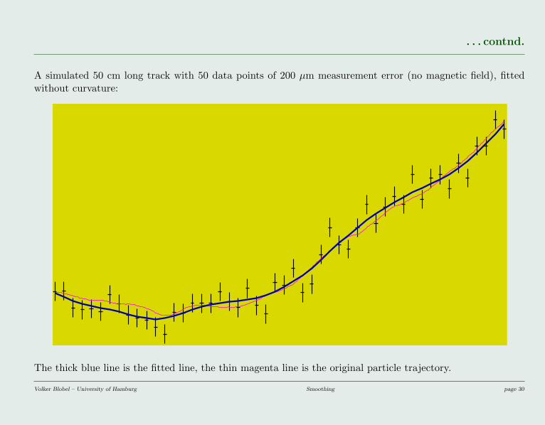
. . . contnd.
A simulated 50 cm long track with 50 data points of 200 µm measurement error (no magnetic field), fittedwithout curvature:
Fit of "random walk" curve
The thick blue line is the fitted line, the thin magenta line is the original particle trajectory.
Volker Blobel – University of Hamburg Smoothing page 30

Curved tracks
The ideal trajectory of a charged particle with momentum p (in GeV/c) and charge e in a constant magneticfield B is a helix, with radius of curvature R and pitch angle λ. The radius of curvature R and the momentumcomponent perpendicular to the direction of the magnetic field are related by
p cos λ = 0.3BR
where B is in Tesla and R is in meters. In the plane perpendicular to the direction of the magnetic field theideal trajectory is part of a circle with radius R. Aim of the track measurement is to determine the curvatureκ ≡ 1/R.
The formalism has now to be modified to describe the superposition of the deflection by the magnetic fieldand the random walk, caused by the multiple scattering.
The segments between the points (xi, ui) and (xi+1, ui+1), which were straight lines in the case on field B = 0,are now curved, with curvature κ. The chord ai of the segment is given by
ai =√
∆x2i + ∆yi with ∆xi = xi+1 − xi ∆yi = yi+1 − yi
≈ ∆xi + 1/2∆y2
i
∆xi
where the latter is a good approximation for ∆xi � ∆yi. The angle γi between the chord and the circle atone end of the chord is given by
γi ≈ sin γi = aiκ/2
and thus in a very good approximation proportional to the curvature κ.
Volker Blobel – University of Hamburg Smoothing page 31

Fit of curved multiple-scattering tracks
A simulated 50 cm long track with 50 data points of 200 µm measurement error in magnetic field, fitted withcurvature:
Fit of "random walk" curve
The thick blue line is the fitted line, the thin magenta line is the original particle trajectory.
Volker Blobel – University of Hamburg Smoothing page 32

. . . contnd.
A simulated 50 cm long track with 50 data points of 200 µm measurement error in magnetic field, fitted withcurvature:
Fit of "random walk" curve
The thick blue line is the fitted line, the thin magenta line is the original particle trajectory.
Volker Blobel – University of Hamburg Smoothing page 33

Fit of curved track with kink
A simulated 50 cm long track with 50 data points of 200 µm measurement error in magnetic field, with akink:
Fit of "random walk" curve
The thick blue line is the fitted line, the thin magenta line is the original particle trajectory.
Volker Blobel – University of Hamburg Smoothing page 34

. . . contnd.
A simulated 50 cm long track with 50 data points of 200 µm measurement error in magnetic field, with akink:
Fit of "random walk" curve
The thick blue line is the fitted line, the thin magenta line is the original particle trajectory.
Volker Blobel – University of Hamburg Smoothing page 35

The new track fit used for outlier rejection . . . H1 CJC data
(1) Track fit with κ and T0 determination . . .Fit of "random walk" curve
(2) . . . down-weighting of first outlier . . .Fit of "random walk" curve
(3) . . . and down-weighting of next outlier . . .Fit of "random walk" curve
(4) . . . finally without outlier.Fit of "random walk" curve
Outliers are hits with > 3σ deviations to fitted line. One outlier is down-weighted at a time.
Volker Blobel – University of Hamburg Smoothing page 36

The same track fit after T0 correction
Three outliers are removed (by down-weighting) and all hits are corrected for the T0, determined in theprevious fit: Fit of "random walk" curve
Volker Blobel – University of Hamburg Smoothing page 37

Smoothing
Why smoothing? 2
Running median smoother 4Single operations . . . . . . . . . . . . . . . . . . . . . 5Combined operations . . . . . . . . . . . . . . . . . . . 6Tracking trends . . . . . . . . . . . . . . . . . . . . . . 7
Orthogonal polynomials 8Straight line fit . . . . . . . . . . . . . . . . . . . . . . 9General orthogonal polynomial . . . . . . . . . . . . . 10Third order polynomial fit . . . . . . . . . . . . . . . . 11Determination of optimal order . . . . . . . . . . . . . 12Least squares smoothing . . . . . . . . . . . . . . . . . 13
Transformations 14
Spline functions 15Cubic splines . . . . . . . . . . . . . . . . . . . . . . . 16B-splines . . . . . . . . . . . . . . . . . . . . . . . . . . 17B-splines with equidistant knots . . . . . . . . . . . . 19Least squares fits of B-splines . . . . . . . . . . . . . . 20
The SPLFT algorithm 21
A new track-fit algorithm 22Multiple scattering . . . . . . . . . . . . . . . . . . . . 23Reconstruction of the trajectory . . . . . . . . . . . . 24The track fit . . . . . . . . . . . . . . . . . . . . . . . 26The solution . . . . . . . . . . . . . . . . . . . . . . . 27Fit of straight multiple-scattering tracks . . . . . . . . 28Curved tracks . . . . . . . . . . . . . . . . . . . . . . . 31Fit of curved multiple-scattering tracks . . . . . . . . 32Fit of curved track with kink . . . . . . . . . . . . . . 34
The new track fit used for outlier rejection . . . . . . . 36The same track fit after T0 correction . . . . . . . . . 37