SMPFRAME: A Distributed Framework for ScheduledModel Parallel Machine Learning

Jin Kyu Kim?, Qirong Ho†, Seunghak Lee?

Xun Zheng?, Wei Dai?, Garth Gibson?, Eric Xing??Carnegie Mellon University, †Institute for Infocomm Research A*STAR

CMU-PDL-15-103

May 2015

Parallel Data LaboratoryCarnegie Mellon UniversityPittsburgh, PA 15213-3890

Acknowledgements: This research is supported in part by Intel as part of the Intel Science and Technology Center for Cloud Comput-ing (ISTC-CC), the National Science Foundation under awards CNS-1042537, CNS-1042543 (PRObE, www.nmc-probe.org), IIS-1447676 (BigData), the National Institute of Health under contract GWAS R01GM087694, and DARPA under contracts FA87501220324 and FA87501220324(XDATA). We thank the members and companies of the PDL Consortium (including Actifio, APC, EMC, Facebook, Google, Hewlett-Packard, Hi-tachi, Huawei, Intel, Microsoft, NetApp, Oracle, Samsung, Seagate, Symantec, Western Digital) for their interest, insights, feedback, and support.

Keywords: Big Data infrastructure, Big Machine Learning systems, Model-Parallel Machine Learning

Abstract

Machine learning (ML) problems commonly applied to big data by existing distributed systems share and update all ML modelparameters at each machine using a partition of data — a strategy known as data-parallel. An alternative and complimentary strategy,model-parallel, partitions model parameters for non-shared parallel access and update, periodically repartitioning to facilitatecommunication. Model-parallelism is motivated by two challenges that data-parallelism does not usually address: (1) parametersmay be dependent, thus naive concurrent updates can introduce errors that slow convergence or even cause algorithm failure;(2) model parameters converge at different rates, thus a small subset of parameters can bottleneck ML algorithm completion. Wepropose scheduled model parallellism (SMP), a programming approach where selection of parameters to be updated (the schedule)is explicitly separated from parameter update logic. The schedule can improve ML algorithm convergence speed by planningfor parameter dependencies and uneven convergence. To support SMP at scale, we develop an archetype software frameworkSMPFRAME which optimizes the throughput of SMP programs, and benchmark four common ML applications written as SMPprograms: LDA topic modeling, matrix factorization, sparse least-squares (Lasso) regression and sparse logistic regression. Byimproving ML progress per iteration through SMP programming whilst improving iteration throughput through SMPFRAME weshow that SMP programs running on SMPFRAME outperform non-model-parallel ML implementations: for example, SMP LDA andSMP Lasso respectively achieve 10x and 5x faster convergence than recent, well-established baselines.

1 Introduction

Machine Learning (ML) algorithms are used to understand and summarize big data, which may be collectedfrom diverse sources such as the internet, industries like finance and banking, or experiments in the physicalsciences, to name a few. The demand for cluster ML implementations is driven by two trends: (1) bigdata: a single machine’s computational power is inadequate with big datasets; (2) large models: withML applications striving for larger numbers of model parameters (at least hundreds of millions [18]),computational power requirements must scale, even if datasets are not too big.

In particular, the trend towards richer, larger ML models with more parameters (up to trillions [20]) isdriven by the need for more “explanatory power”: it has been observed that big datasets contain “longer tails”,rare-yet-unique events, than smaller datasets, and detection of such events can be crucial to downstreamtasks [33, 31]. Many of these big models are extremely slow to converge when trained with a sequentialalgorithm, leading to model-parallelism [8, 19, 33, 21], which as the name suggests, splits ML modelparameters across machines, and makes each machine responsible for updating only its assigned parameters(either using the full data, or a data subset). Even when the model is relatively small, model-parallel executioncan still mean the difference between hours or days of compute on a single machine, versus minutes on acluster [5, 30].

Model-parallelism can be contrasted with data-parallelism, where each machine gets one partition ofthe data, and iteratively generates sub-updates that are applied to all ML model parameters, until convergenceis reached. This is possible because most ML algorithms assume data independence under the model —independent and identically distributed data in statistical parlance — and as a result, all machines’ sub-updatescan be easily combined, provided every machine has access to the same global model parameters.

This convenient property does not apply to model-parallel algorithms, which introduce new subtleties:(1) unlike data samples, the model parameters are not independent, and (2) model parameters may takedifferent numbers of iterations to converge (uneven convergence). Hence, the effectiveness of a model-parallelalgorithm is greatly affected by its schedule: which parameters are updated in parallel, and how they areprioritized [21, 37].

Poorly-chosen schedules decrease the progress made by each ML algorithm iteration, or may evencause the algorithm to fail. Note that progress per iteration is distinct from iteration throughput (number ofiterations executed per unit time); effective ML implementations combine high progress per iteration withhigh iteration throughput, yielding high progress per unit time. Despite these challenges, model-parallelalgorithms have shown promising speedups over their data-parallel counterparts [33, 31].

In the ML literature, there is a strong focus on verifying the safety or correctness of parallel algorithms viastatistical theory [5, 23, 38], but this is often done under simple assumptions about distributed environments— for example, network communication and synchronization costs are often ignored. On the other hand, thesystems literature is focused on developing distributed systems [9, 34, 20, 22], with high-level programminginterfaces that allow ML developers to focus on the ML algorithm’s core routines. Some of these systemsenjoy strong fault tolerance and synchronization guarantees that ensure correct ML execution [9, 34], whileothers [16, 20] exploit the error-tolerance of data-parallel ML algorithms, and employ relaxed synchronizationguarantees in exchange for higher iterations-per-second throughput. In nearly all of these systems, the MLalgorithm is treated as a black box, with little opportunity to control the parallel schedule of updates (in thesense that we defined earlier). As a result, these systems offer little support for model-parallel ML algorithms,in which it is often vital to re-schedule updates in response to model parameter dependencies and unevenconvergence.

These factors paint an overall picture of model-parallel ML that is at once promising, yet under-supportedfrom the following angles: (1) limited understanding of model-parallel execution order, and how it canimprove the speed of model-parallel algorithms; (2) limited systems support to investigate and developbetter model-parallel algorithms; (3) limited understanding of the safety and correctness of model-parallel

1

algorithms under realistic systems conditions. To address these challenges, this paper proposes scheduledmodel parallelism (SMP), where an ML application scheduler generates model-parallel schedules thatimprove model-parallel algorithm progress per update, by considering dependency structures and prioritizingparameters. Essentially, SMP allows model-parallel algorithms to be separated into a control componentresponsible for dependency checking and priortization, and an update component that executes iterative MLupdates in the parallel schedule prescribed by the control component.

To realize SMP, we develop a prototype SMP framework called SMPFRAME that parallelizes SMPML applications over a cluster. While SMP maintains high progress per iteration, the SMPFRAME softwareimproves iterations executed per second, by (1) pipelining SMP iterations, (2) overlapping SMP computationwith parameter synchronization over the network, and (3) streaming computations over a ring topology.Through SMP on top of SMPFRAME, we achieve high parallel ML performance through increased progressper iteration, as well as increased iterations per second — the result is substantially increased progress persecond, and therefore faster ML algorithm completion. We benchmark various SMP algorithms implementedon SMPFRAME — Gibbs sampling for topic modeling [4, 15], stochastic gradient descent for matrixfactorization [12], and coordinate descent for sparse linear (i.e., Lasso [28, 10]) and logistic [11] regressions— and show that SMP programs on SMPFRAME outperform non-model parallel ML implementations.

2 Model Parallelism

Although machine learning problems exhibit a diverse spectrum of model forms, such as probabilistic topicmodels, optimization-theoretic regression formulations, etc., their algorithmic solutions implemented bya computer program typically take the form of an iterative convergent procedure, meaning that they areoptimization or Markov Chain Monte Carlo (MCMC [29]) algorithms that repeat some set of fixed-pointupdate routines until convergence (i.e. a stopping criterion has been reached):

A(t) = A(t−1) + ∆(D,A(t−1)), (1)

where index t refers to the current iteration, A are the model parameters, D is the input data, and ∆() isthe model update function 1. Such iterative-convergent algorithms have special properties that we shallexplore: tolerance to (non-recursive) errors in model state during iteration, dependency structures that mustbe respected during parallelism, and uneven convergence across model parameters.

In model-parallel ML programs, parallel workers recursively update subsets of model parameters untilconvergence — this is in contrast to data-parallel programs, which parallelize over subsets of data samples. Amodel-parallel ML program extends Eq. (1) to the following form:

A(t) = A(t−1) +∑P

p=1 ∆p(D,A(t−1), Sp(D,A

(t−1))),

where ∆p() is the model update function executed at parallel worker p. The “schedule” Sp() outputs a subsetof parameters in A, which tells the p-th parallel worker which parameters it should work on sequentially(i.e. workers may not further parallelize within Sp()). Since the data D is unchanging, we drop it from thenotation for clarity:

A(t) = A(t−1) +∑P

p=1 ∆p(A(t−1), Sp(A

(t−1))). (2)

Parallel coordinate descent solvers are a good example of model parallelism, and have been applied withgreat success to the Lasso sparse regression problem [5]. In addition, MCMC or sampling algorithms can also

1The summation between ∆() and A(t−1) can be generalized to a general aggregation function F (A(t−1),∆()); for concretenesswe restrict our attention to the summation form, but the techniques proposed in this paper can be applied to F .

2

be model-parallel: for example, the Gibbs sampling algorithm normally processes one model parameter at atime, but it can be run in parallel over many variables at once, as seen in topic model implementations [13, 33].Unlike data-parallel algorithms which parallelize over independent data samples, model-parallel algorithmsparallelize over model parameters that are, in general, not independent; this can cause poor performance (orsometimes even algorithm failure) if not handled with care [5, 25], and usually necessitate approaches andtheories very different from that of data parallelism, which is our main focus in this paper.

2.1 Properties of ML AlgorithmsSome intrinsic properties of ML algorithms (i.e., Eq. (1)) can provide new opportunities for effectiveparallelism when correctly explored: (1) Model Dependencies, which refers to the phenomenon that differentelements in A are coupled, meaning that an update to one element will strongly influence the next update toanother parameter. If such dependencies are violated, which is typical during random parallelization, they willincur errors to the ML algorithm’s progress, leading to reduced convergence speed (or even algorithm failure)when we increase the degree of parallelism [5]. Furthermore, not all model dependencies are explicitlyspecified in an ML program, meaning that they have to be computed from data, such as in Lasso [5]. (2)Uneven Convergence, which means different model parameters may converge at different rates, leading tonew speedup opportunities via parameter prioritization [21, 37]. Finally, (3) Error-Tolerant — a limitedamount of stochastic error during computation of ∆(D,At−1) in each iteration does not lead to algorithmfailure (though it might slow down convergence speed).

Sometimes, it is not practical or possible to find a “perfect” parallel execution scheme for an MLalgorithm, which means that some dependencies will be violated, leading to incorrect update operations.But, unlike classical computer science algorithms where incorrect operations always lead to failure, iterative-convergent ML programs (also known as “fixed-point iteration” algorithms) can be thought of as having abuffer to absorb inaccurate updates or other errors, and will not fail as long as the buffer is not overrun. Evenso, there is a strong incentive to minimize errors: the more dependencies the system finds and avoids, themore progress the ML algorithm will make each iteration — unfortunately, finding those dependencies mayincur non-trivial computational costs, leading to reduced iteration throughput. Because an ML program’sconvergence speed is essentially progress per iteration multiplied by iteration throughput, it is important tobalance these two considerations. Below, we explore this idea by explicitly discussing some variations withinmodel parallelism, in order to expose possible ways by which model parallelization can be made efficient.

2.2 Variations of Model-ParallelismWe restrict our attention to model-parallel programs that partition M model parameters across P workerthreads in an approximately load-balanced manner; highly unbalanced partitions are inefficient and un-desirable. Here, we introduce variations on model-parallelism, which differ on their partitioning quality.Concretely, partitioning involves constructing a size-M2 dependency graph, with weighted edges eij thatmeasure the dependency between parameters Ai and Aj . This measure of dependency differs from algorithmto algorithm: e.g., in Lasso regression eij is the correlation between the i-th and j-th data dimensions. Thetotal violation of a partitioning is the sum of weights of edges that cross between the P partitions, and wewish to minimize this.

Ideal Model-Parallel: Theoretically, there exists an “ideal” load-balanced parallelization over Pworkers which gives the highest possible progress per iteration; this is indicated by an ideal (but notnecessarily computable) schedule Sidealp () that replaces the generic Sp() in Eq. (2). There are two pointsto note: (1) even this “ideal” model parallelization can still violate model dependencies and incur errors,compared to sequential execution because of residue cross-worker coupling; (2) computing Sidealp () isexpensive in general because graph-partitioning is NP-hard. Ideal model parallelization achieves the highestprogress per iteration amongst load-balanced model-parallel programs, but may incur a large one-time oreven every-iteration partitioning cost, which can greatly reduce iteration throughput.

3

Random Model-Parallel: At the other extreme is random model-parallelization, in which a scheduleSrandp () simply chooses one parameter at random for each worker p [5]. As the number of workers Pincreases, the expected number of violated dependencies will also increase, leading to poor progress periteration (or even algorithm failures). However, there is practically no cost to iteration throughput.

Approximate Model-Parallel: As a middle ground between ideal and random model-parallelization, wemay approximate Sidealp () via a cheap-to-compute scheduleSapproxp (). A number of strategies exist: one may partition small subsets of parameters at a time (in-stead of the M2-size full dependency graph), or apply approximate partitioning algorithms [26] such asMETIS [17] (to avoid NP-hard partitioning costs), or even use strategies that are unique to a particular MLprogram’s structure.

In this paper, our goal is to explore strategies for efficient and effective approximate model parallelization.We focus on ideas for generating model partitions and schedules:

Static Partitioning: A fixed, static schedule Sfixp () hard-codes the partitioning for every iteration before-hand. Progress per iteration varies depending on how well Sfixp () matches the ML program’s dependencies,but like random model-parallel, this has little cost to iteration throughput.

Dynamic Partitioning: Dynamic partitioning Sdynp () tries to select independent parameters for eachworker, by performing pair-wise dependency tests between a small number L of parameters (which can bechosen differently at different iterations, based on some priority policy as discussed later); the GraphLabsystem achieves a similar outcome via graph consistency models [21]. The idea is to only do L2 computationalwork per iteration, which is far less than M2 (where M is the total number of parameters), based on a prioritypolicy that selects the L parameters that matter most to the program’s convergence. Dynamic partitioning canachieve high progress per iteration, similar to ideal model-parallelism, but may suffer from poor iterationthroughput on distributed clusters: because only a small number of parameters are updated each iteration,the time spent computing ∆p() at the P workers cannot amortize away network latencies and the cost ofcomputing Sdynp ().

Pipelining: This is not a different type of model-parallelism per se, but a complementary technique thatcan be applied to any model-parallel strategy. Pipelining allows the next iteration(s) to start before the currentone finishes, ensuring that computation is always fully utilized; however, this introduces staleness into themodel-parallel execution:

A(t) = A(t−1) +∑P

p=1 ∆p(A(t−s), Sp(A

(t−s))). (3)

Note how the model parameters A(t−s) being used for ∆p(), Sp() come from iteration (t− s), where s is thepipeline depth. Because ML algorithms are error-tolerant, they can still converge under stale model images(up to a practical limit) [16, 7]. Pipelining therefore sacrifices some progress per iteration to increase iterationthroughput, and is a good way to raise the throughput of dynamic partitioning.

Prioritization: Like pipelining, prioritization is complementary to model-parallel strategies. The ideais to modify Sp() to prefer parameters that, when updated, will yield the most convergence progress [21],while avoiding parameters that are already converged [20]; this is effective because ML algorithms exhibituneven parameter convergence. Since computing a parameter’s potential progress can be expensive, we mayemploy cheap-but-effective approximations or heuristics to estimate the potential progress (as shown later).Prioritization can thus greatly improve progress per iteration, at a small cost to iteration throughput.

2.3 Scheduled Model Parallelism for Programming

Model-parallelism accommodates a wide range of partitioning and prioritization strategies (i.e. the scheduleSp()), from simple random selection to complex, dependency-calculating functions that can be more expensivethan the updates ∆p(). In existing ML program implementations, the schedule is often written as part of the

4

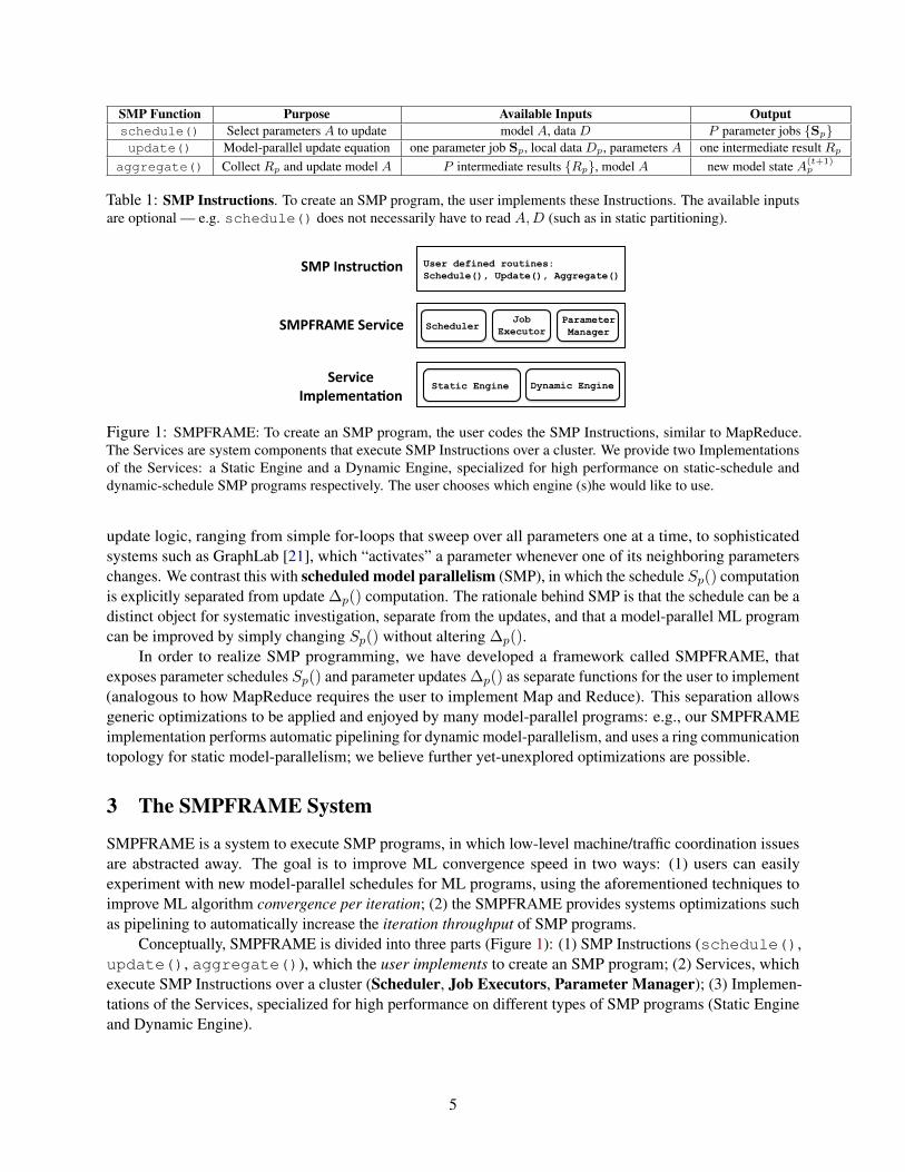
SMP Function Purpose Available Inputs Outputschedule() Select parameters A to update model A, data D P parameter jobs {Sp}update() Model-parallel update equation one parameter job Sp, local data Dp, parameters A one intermediate result Rp

aggregate() Collect Rp and update model A P intermediate results {Rp}, model A new model state A(t+1)p

Table 1: SMP Instructions. To create an SMP program, the user implements these Instructions. The available inputsare optional — e.g. schedule() does not necessarily have to read A,D (such as in static partitioning).

SMP  Instruc,on  

SMPFRAME  Service  

Service    Implementa,on  

User defined routines: Schedule(), Update(), Aggregate()

Scheduler Job

Executor Parameter Manager

Static Engine Dynamic Engine

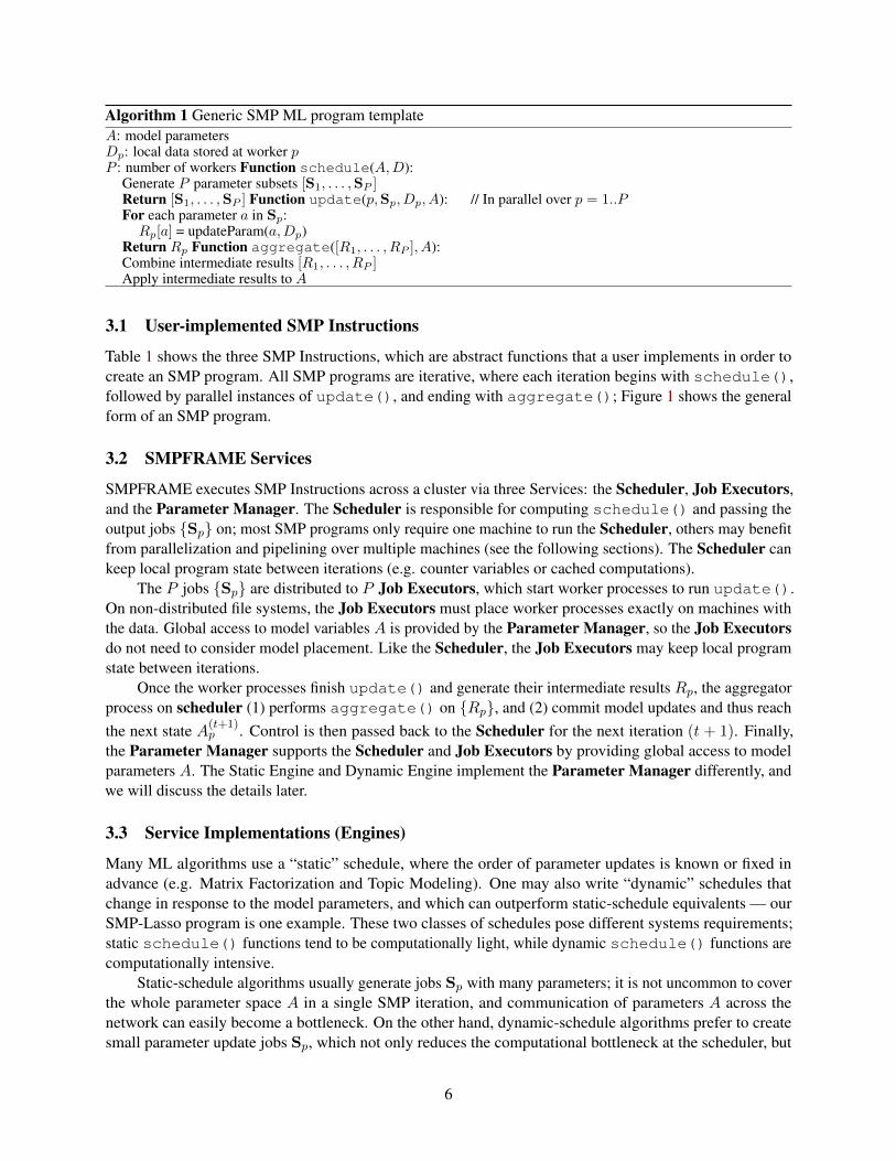
Figure 1: SMPFRAME: To create an SMP program, the user codes the SMP Instructions, similar to MapReduce.The Services are system components that execute SMP Instructions over a cluster. We provide two Implementationsof the Services: a Static Engine and a Dynamic Engine, specialized for high performance on static-schedule anddynamic-schedule SMP programs respectively. The user chooses which engine (s)he would like to use.

update logic, ranging from simple for-loops that sweep over all parameters one at a time, to sophisticatedsystems such as GraphLab [21], which “activates” a parameter whenever one of its neighboring parameterschanges. We contrast this with scheduled model parallelism (SMP), in which the schedule Sp() computationis explicitly separated from update ∆p() computation. The rationale behind SMP is that the schedule can be adistinct object for systematic investigation, separate from the updates, and that a model-parallel ML programcan be improved by simply changing Sp() without altering ∆p().

In order to realize SMP programming, we have developed a framework called SMPFRAME, thatexposes parameter schedules Sp() and parameter updates ∆p() as separate functions for the user to implement(analogous to how MapReduce requires the user to implement Map and Reduce). This separation allowsgeneric optimizations to be applied and enjoyed by many model-parallel programs: e.g., our SMPFRAMEimplementation performs automatic pipelining for dynamic model-parallelism, and uses a ring communicationtopology for static model-parallelism; we believe further yet-unexplored optimizations are possible.

3 The SMPFRAME System

SMPFRAME is a system to execute SMP programs, in which low-level machine/traffic coordination issuesare abstracted away. The goal is to improve ML convergence speed in two ways: (1) users can easilyexperiment with new model-parallel schedules for ML programs, using the aforementioned techniques toimprove ML algorithm convergence per iteration; (2) the SMPFRAME provides systems optimizations suchas pipelining to automatically increase the iteration throughput of SMP programs.

Conceptually, SMPFRAME is divided into three parts (Figure 1): (1) SMP Instructions (schedule(),update(), aggregate()), which the user implements to create an SMP program; (2) Services, whichexecute SMP Instructions over a cluster (Scheduler, Job Executors, Parameter Manager); (3) Implemen-tations of the Services, specialized for high performance on different types of SMP programs (Static Engineand Dynamic Engine).

5

Algorithm 1 Generic SMP ML program templateA: model parametersDp: local data stored at worker pP : number of workers Function schedule(A,D):

Generate P parameter subsets [S1, . . . ,SP ]Return [S1, . . . ,SP ] Function update(p,Sp, Dp, A): // In parallel over p = 1..PFor each parameter a in Sp:Rp[a] = updateParam(a,Dp)

Return Rp Function aggregate([R1, . . . , RP ], A):Combine intermediate results [R1, . . . , RP ]Apply intermediate results to A

3.1 User-implemented SMP Instructions

Table 1 shows the three SMP Instructions, which are abstract functions that a user implements in order tocreate an SMP program. All SMP programs are iterative, where each iteration begins with schedule(),followed by parallel instances of update(), and ending with aggregate(); Figure 1 shows the generalform of an SMP program.

3.2 SMPFRAME Services

SMPFRAME executes SMP Instructions across a cluster via three Services: the Scheduler, Job Executors,and the Parameter Manager. The Scheduler is responsible for computing schedule() and passing theoutput jobs {Sp} on; most SMP programs only require one machine to run the Scheduler, others may benefitfrom parallelization and pipelining over multiple machines (see the following sections). The Scheduler cankeep local program state between iterations (e.g. counter variables or cached computations).

The P jobs {Sp} are distributed to P Job Executors, which start worker processes to run update().On non-distributed file systems, the Job Executors must place worker processes exactly on machines withthe data. Global access to model variables A is provided by the Parameter Manager, so the Job Executorsdo not need to consider model placement. Like the Scheduler, the Job Executors may keep local programstate between iterations.

Once the worker processes finish update() and generate their intermediate results Rp, the aggregatorprocess on scheduler (1) performs aggregate() on {Rp}, and (2) commit model updates and thus reachthe next state A(t+1)

p . Control is then passed back to the Scheduler for the next iteration (t + 1). Finally,the Parameter Manager supports the Scheduler and Job Executors by providing global access to modelparameters A. The Static Engine and Dynamic Engine implement the Parameter Manager differently, andwe will discuss the details later.

3.3 Service Implementations (Engines)

Many ML algorithms use a “static” schedule, where the order of parameter updates is known or fixed inadvance (e.g. Matrix Factorization and Topic Modeling). One may also write “dynamic” schedules thatchange in response to the model parameters, and which can outperform static-schedule equivalents — ourSMP-Lasso program is one example. These two classes of schedules pose different systems requirements;static schedule() functions tend to be computationally light, while dynamic schedule() functions arecomputationally intensive.

Static-schedule algorithms usually generate jobs Sp with many parameters; it is not uncommon to coverthe whole parameter space A in a single SMP iteration, and communication of parameters A across thenetwork can easily become a bottleneck. On the other hand, dynamic-schedule algorithms prefer to createsmall parameter update jobs Sp, which not only reduces the computational bottleneck at the scheduler, but

6

scheduler  

D1  A1  

D2  A2  

D3  A3  

D4  A4  

S1  

S2  

S3  

S4  

R1  

R2  R3  

R4  

JobExecutor-­‐1  

JobExecutor-­‐3  

JobExecutor-­‐2  

JobExecutor-­‐4  

(a) Ring topology

Parameter    

Manager  

Job  Po

ol  

Manager  

Update  Thread  

Update  Thread  

Update  Thread  

Job  InQ  

OutQ  

Update  Thread  

Update  Thread  

In-­‐Port  

Out-­‐Port  

(b) Job Executor

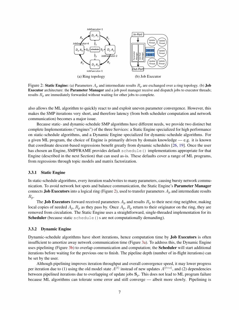
Figure 2: Static Engine: (a) Parameters Ap and intermediate results Rp are exchanged over a ring topology. (b) JobExecutor architecture: the Parameter Manager and a job pool manager receive and dispatch jobs to executor threads;results Rp are immediately forwarded without waiting for other jobs to complete.

also allows the ML algorithm to quickly react to and exploit uneven parameter convergence. However, thismakes the SMP iterations very short, and therefore latency (from both scheduler computation and networkcommunication) becomes a major issue.

Because static- and dynamic-schedule SMP algorithms have different needs, we provide two distinct butcomplete Implementations (“engines”) of the three Services: a Static Engine specialized for high performanceon static-schedule algorithms, and a Dynamic Engine specialized for dynamic-schedule algorithms. Fora given ML program, the choice of Engine is primarily driven by domain knowledge — e.g. it is knownthat coordinate descent-based regressions benefit greatly from dynamic schedules [26, 19]. Once the userhas chosen an Engine, SMPFRAME provides default schedule() implementations appropriate for thatEngine (described in the next Section) that can used as-is. These defaults cover a range of ML programs,from regressions through topic models and matrix factorization.

3.3.1 Static Engine

In static-schedule algorithms, every iteration reads/writes to many parameters, causing bursty network commu-nication. To avoid network hot spots and balance communication, the Static Engine’s Parameter Managerconnects Job Executors into a logical ring (Figure 2), used to transfer parametersAp and intermediate resultsRp.

The Job Executors forward received parameters Ap and results Rp to their next ring neighbor, makinglocal copies of needed Ap, Rp as they pass by. Once Ap, Rp return to their originator on the ring, they areremoved from circulation. The Static Engine uses a straightforward, single-threaded implementation for itsScheduler (because static schedule()s are not computationally demanding).

3.3.2 Dynamic Engine

Dynamic-schedule algorithms have short iterations, hence computation time by Job Executors is ofteninsufficient to amortize away network communication time (Figure 3a). To address this, the Dynamic Engineuses pipelining (Figure 3b) to overlap communication and computation; the Scheduler will start additionaliterations before waiting for the previous one to finish. The pipeline depth (number of in-flight iterations) canbe set by the user.

Although pipelining improves iteration throughput and overall convergence speed, it may lower progressper iteration due to (1) using the old model state A(t) instead of new updates A(t+s), and (2) dependenciesbetween pipelined iterations due to overlapping of update jobs Sp. This does not lead to ML program failurebecause ML algorithms can tolerate some error and still converge — albeit more slowly. Pipelining is

7

Master  Scheduler  

Scheduler-­‐1  

Scheduler-­‐2  

Job  Executors  

scheduling   aggrega9on   job  execu9on  

{Tt}   {Rt}   {Tt+1}   {Rt+1}   {Tt+2}   {Rt+2}  

{Tt+1}  

{Tt+2}  

{Tt+3}  

(a) Non-pipelined

Master  Scheduler  

Scheduler-­‐1  

Scheduler-­‐3  

Job  Executors  

{Rt}  

Scheduler-­‐2  

{Tt}   {Tt+1}   {Tt+2}   {Tt+3}   {Tt+4}   {Tt+5}  

{Rt+1}  {Rt+2}   {Rt+3}  {Rt+4}   {Rt+5}  

scheduling   aggrega:on   job  execu:on  

(b) Pipelined

Figure 3: Dynamic Engine pipelining: (a) Non-pipelined execution: network latency dominates; (b) Pipeliningoverlaps networking and computation.

basically execution with stale parameters, A(t) = F (A(t−s), {∆p(A(t−s), Sp(A

(t−s)))}Pp=1) where s is thepipeline depth.

3.4 Other Considerations

Fault tolerance: SMPFRAME execution can be made fault-tolerant, by checkpointing the model parametersA every x iterations. Because ML programs are error-tolerant, background checkpointing (which may spanseveral iterations), is typically sufficient.Avoiding lock contention: To avoid lock contention, the SMPFRAME Scheduler and Job Executors avoidsharing data structures between threads in the same process. For example, when jobs Sp are being assignedby a Job Executor process to individual worker threads, we use a separate, dedicated queue for each workerthread.Dynamic Engine parameter reordering: Within each Dynamic Engine iteration, SMPFRAME re-ordersthe highest priority parameters to the front of the iteration, which improves the performance of pipelining.The intuition is as follows: because high-priority parameters have a larger effect on subsequent iterations,we should make their updated values available as soon as possible, rather than waiting until the end of thepipeline depth s.

4 SMP Implementations of ML Programs

We describe how two ML algorithms can be written as Scheduled Model Parallel (SMP) programs. Theuser implements schedule(), update(), aggregate(); alternatively, SMPFRAME provides pre-implemented schedule() functions for some classes of SMP programs. Algorithm 1 shows a typical SMPprogram.

4.1 Parallel Coordinate Descent for Lasso

Lasso, or `1-regularized least-squares regression, is used to identify a small set of important features fromhigh-dimensional data. It is an optimization problem

minβ12

∑ni=1

(yi − xiβ

)2+ λ‖β‖1 (4)

where ‖β‖1 =∑d

a=1 |βa| is a sparsity-inducing `1-regularizer, and λ is a tuning parameter that controlsthe sparsity level of w. X is an N -by-M design matrix (xi represents the i-th row, xa represents the a-thcolumn), y is an N -by-1 observation vector, and β is the M -by-1 coefficient vector (the model parameters).The Coordinate Descent (CD) algorithm is used to solve Eq. (4), and thus learn β from the inputs X,y; the

8

Algorithm 2 SMP Dynamic, Prioritized LassoX,y: input data{X}p, {y}p: rows/samples of X,y stored at worker pβ: model parameters (regression coefficients)λ: `1 regularization penaltyτ : G edges whose weight is below τ are ignored

Function schedule(β,X):Pick L > P params in β with probability ∝ (∆βa)2

Build dependency graph G over L chosen params:edge weight of (βa, βb) = correlation(xa,xb)

[βG1 , . . . , βGK] = findIndepNodeSet(G, τ )

For p = 1..P :Sp = [βG1 , . . . , βGK

]Return [S1, . . . ,SP ]

Function update(p,Sp, {X}p, {y}p, β):For each param βa in Sp, each row i in {X}p:Rp[a] += xiay

i −∑

b 6=a xiax

ibβb

Return Rp

Function aggregate([R1, . . . , RP ],S1, β):For each parameter βa in S1:

temp =∑P

p=1Rp[a]

βa = S(temp, λ)

CD update rule for βa is

β(t)a ← S(x>a y −

∑b6=a x

>a xbβ

(t−1)b , λ), (5)

where S(·, λ) is a soft-thresholding operator [10].Algorithm 2 shows an SMP Lasso that uses dynamic, prioritized scheduling. It expects that each machine

locally stores a subset of data samples (which is common practice in cluster ML), however the Lasso updateEq. (5) uses a feature/column-wise access pattern. Therefore every worker p = 1..P operates on the samescheduled set of L parameters, but using their respective data partitions {X}p, {y}p. Note that update()and aggregate() are a straightforward implementation of Eq. (5).

We direct attention to schedule(): it picks (i.e. prioritizes) L parameters in β with probabilityproportional to their squared difference from the latest update (their “delta”); parameters with larger delta aremore likely to be non-converged. Next, it builds a dependency graph over these L parameters, with edgeweights equal to the correlation2 between data columns xa,xb. Finally, it removes all edges in G below athreshold τ > 0, and extracts nodes βGk that do not have common edges. All chosen βGk are thus pairwiseindependent and safe to update in parallel.

Why is such a sophisticated schedule() necessary? Suppose we used random parameter selection [5]:Figure 4 shows its progress, on the Alzheimer’s Disease (AD) data [36]. The total compute to reach a fixedobjective value goes up with more concurrent updates — i.e. progress per unit computation is decreasing, andthe algorithm has poor scalability. Another reason is uneven parameter convergence: Figure 5 shows howmany iterations different parameters took to converge on the AD dataset; > 85% of parameters converged in< 5 iterations, suggesting that the prioritization in Algorithm 2 should be very effective.Default schedule() functions: The squared delta-based parameter prioritization and dynamic depen-dency checking in SMP Lasso’s schedule() (Algorithm 2) generalize to other regression problems — forexample, we also implement sparse logistic regression using the same schedule(). SMPFRAME allowsML programmers to re-use Algorithm 2’s schedule() via a library function scheduleDynRegr().

2On large data, it suffices to estimate the correlation with a data subsample.

9

0.0015 0.002

0.0025 0.003

0.0035 0.004

2000 4000obje

ctiv

e va

lue

data processed (1K)

degree of parallelism 3264

128256

Figure 4: Random Model-Parallel Lasso: Objective value (lower the better) versus processed data samples, with 32to 256 workers performing concurrent updates. Under naive (random) model-parallel, higher degree of parallelismresults in worse progress.

λ:0.0001 λ:0.001 λ:0.01

84.72% 95.32% 98.23%

1000000

100000

10000

1000

100

5 20 40 60 80 100 5 20 40 60 80 100 5 20 40 60 80 100

# o

f co

nve

rge

d p

aram

ete

rs

Iterations

Figure 5: Uneven Parameter Convergence: Number of converged parameters at each iteration, with differentregularization parameters λ. Red bar shows the percentage of converged parameters at iteration 5.

4.2 Parallel Gibbs Sampling for Topic Modeling

Topic modeling, a.k.a. Latent Dirichlet Allocation (LDA), is an ML model for document soft-clustering; itassigns each of N text documents to a probability distribution over K topics, and each topic is a distributionover highly-correlated words. Topic modeling is usually solved via a parallel Gibbs sampling algorithm,involving three data structures: an N -by-K document-topic table U , an M -by-K word-topic table V (whereM is the vocabulary size), and the topic assignments zij to each word “token” j in each document i. Eachtopic assignment zij is associated with the j-th word in the i-th document, wij (an integer in 1 through M );the zij , wij are usually pre-partitioned over worker machines [1].

The Gibbs sampling algorithm iteratively sweeps over all zij , assigning each one a new topic via thisprobability distribution over topic outcomes k = 1..K:

P (zij = k | U, V ) ∝ α+Uik

Kα+∑K

`=1 Ui`+

β+Vwij,k

Mβ+∑M

m=1 Vmk, (6)

where α, β are smoothing parameters. Once a new topic for zij has been sampled, the tables U, V are updatedby (1) decreasing Vi,oldtopic and Uwij ,oldtopic by one, and (2) increasing Ui,newtopic and Vwij ,newtopic by one.

Eq. (6) is usually replaced by a more efficient (but equivalent) variant called SparseLDA [32], whichwe also use. We will not show its details within update() and aggregate(); instead, we focus on howschedule() controls which zij are being updated by which worker. Algorithm 3 shows our SMP LDAimplementation, which uses a static “word-rotation” schedule, and partitions the documents over workers.The word-rotation schedule partitions the rows of V (word-topic table), so that workers never touch thesame rows in V (each worker just skips over words wij associated with not-assigned rows). The partitioningis “rotated” P times, so that every word wij in each worker is touched exactly once after P invocations ofschedule().

As with Lasso, one might ask why this schedule() is useful. A common strategy is to have workerssweep over all their zij every iteration [1], however, as we show later in Sec 6, this causes concurrent writesto the same rows in V , breaking model dependencies.

10

Algorithm 3 SMP Static-schedule Topic ModelingU, V : doc-topic table, word-topic table (model params)N,M : number of docs, vocabulary size{z}p, {w}p: topic indicators and token words stored at worker pc: persistent counter in schedule() Function schedule():

For p = 1..P : // “word-rotation” schedulex = (p− 1 + c) mod PSp = (xM/P, (x+ 1)M/P ) // p’s word range

c = c+ 1Return [S1, . . . ,SP ] Function update(p,Sp, {U}p, V, {w}p, {z}p):[lower,upper] = Sp // Only touch wij in rangeFor each token zij in {z}p:

If wij ∈ range(lower,upper):old = zijnew = SparseLDAsample(Ui, V, wij , zij)Record old, new values of zij in Rp

Return Rp Function aggregate([R1, . . . , RP ], U, V ):Update U, V with changes in [R1, . . . , RP ]

Default schedule() functions: Like SMP Lasso, SMP LDA’s schedule() (Algorithm 3) can be gener-ically applied to ML program where each data sample touches just a few parameters (Matrix Factorizationis one example). The idea is to assign disjoint parameter subsets across workers, who only operate on datasamples that “touch” their currently assigned parameter subset. For this purpose, SMPFRAME provides ageneric scheduleStaticRota() that partitions the parameters into P contiguous (but disjoint) blocks,and rotates these blocks amongst workers at the beginning of each iteration.

4.3 Other ML Programs

In our evaluation, we consider two more SMP ML Programs — sparse Logistic Regression (SLR) and MatrixFactorization (MF). SMP SLR uses the same dynamic, prioritized scheduleDynRegr() as SMP Lasso,while the update() and aggregate() functions are slightly different to accommodate the new LRobjective function. SMP MF uses scheduleStaticRota() that, like SMP LDA, rotates disjoint (andtherefore dependency-free) parameter assignments amongst the P distributed workers.

5 SMP Theoretical Guarantees

SMP programs are iterative-convergent algorithms that follow the general model-parallel Eq. (2). Here, webriefly state guarantees about their execution. SMP programs with static schedules are covered by existingML analysis [5, 26].

Theorem 1 Dynamic scheduling converges: Recall the Lasso Algorithm 2. Let ε := (P−1)(ρ−1)M < 1,

where P is the number of parallel workers, M is the number of features (columns of the design matrix X),and ρ is the “spectral radius” of X. After t iterations, we have

E[F (β(t))− F (β?)] ≤ CM

P (1− ε)1

t= O

(1

t

), (7)

where F (β) is the Lasso objective function Eq. (4), β? is an optimal solution to F (β), and C is a constantspecific to the dataset (X,y) that subsumes the spectral radius ρ, as well as the correlation threshold τ inAlgorithm 2. The proof can be generalized to other coordinate descent programs.

11

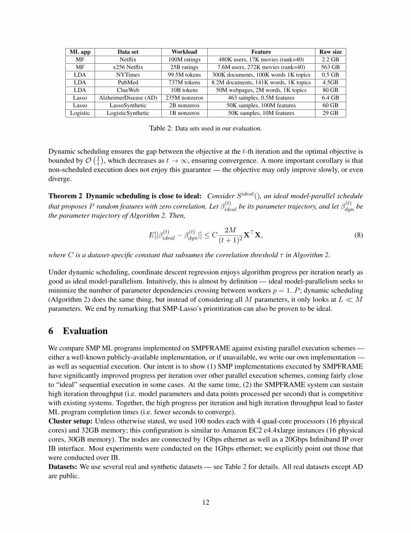
ML app Data set Workload Feature Raw sizeMF Netflix 100M ratings 480K users, 17K movies (rank=40) 2.2 GBMF x256 Netflix 25B ratings 7.6M users, 272K movies (rank=40) 563 GB

LDA NYTimes 99.5M tokens 300K documents, 100K words 1K topics 0.5 GBLDA PubMed 737M tokens 8.2M documents, 141K words, 1K topics 4.5GBLDA ClueWeb 10B tokens 50M webpages, 2M words, 1K topics 80 GBLasso AlzheimerDisease (AD) 235M nonzeros 463 samples, 0.5M features 6.4 GBLasso LassoSynthetic 2B nonzeros 50K samples, 100M features 60 GB

Logistic LogisticSynthetic 1B nonzeros 50K samples, 10M features 29 GB

Table 2: Data sets used in our evaluation.

Dynamic scheduling ensures the gap between the objective at the t-th iteration and the optimal objective isbounded by O

(1t

), which decreases as t→∞, ensuring convergence. A more important corollary is that

non-scheduled execution does not enjoy this guarantee — the objective may only improve slowly, or evendiverge.

Theorem 2 Dynamic scheduling is close to ideal: Consider Sideal(), an ideal model-parallel schedulethat proposes P random features with zero correlation. Let β(t)ideal be its parameter trajectory, and let β(t)dyn bethe parameter trajectory of Algorithm 2. Then,

E[|β(t)ideal − β(t)dyn|] ≤ C

2M

(t+ 1)2X>X, (8)

where C is a dataset-specific constant that subsumes the correlation threshold τ in Algorithm 2.

Under dynamic scheduling, coordinate descent regression enjoys algorithm progress per iteration nearly asgood as ideal model-parallelism. Intuitively, this is almost by definition — ideal model-parallelism seeks tominimize the number of parameter dependencies crossing between workers p = 1..P ; dynamic scheduling(Algorithm 2) does the same thing, but instead of considering all M parameters, it only looks at L � Mparameters. We end by remarking that SMP-Lasso’s prioritization can also be proven to be ideal.

6 Evaluation

We compare SMP ML programs implemented on SMPFRAME against existing parallel execution schemes —either a well-known publicly-available implementation, or if unavailable, we write our own implementation —as well as sequential execution. Our intent is to show (1) SMP implementations executed by SMPFRAMEhave significantly improved progress per iteration over other parallel execution schemes, coming fairly closeto “ideal” sequential execution in some cases. At the same time, (2) the SMPFRAME system can sustainhigh iteration throughput (i.e. model parameters and data points processed per second) that is competitivewith existing systems. Together, the high progress per iteration and high iteration throughput lead to fasterML program completion times (i.e. fewer seconds to converge).Cluster setup: Unless otherwise stated, we used 100 nodes each with 4 quad-core processors (16 physicalcores) and 32GB memory; this configuration is similar to Amazon EC2 c4.4xlarge instances (16 physicalcores, 30GB memory). The nodes are connected by 1Gbps ethernet as well as a 20Gbps Infiniband IP overIB interface. Most experiments were conducted on the 1Gbps ethernet; we explicitly point out those thatwere conducted over IB.Datasets: We use several real and synthetic datasets — see Table 2 for details. All real datasets except ADare public.

12

-1.45

-1.4

-1.35

-1.3

-1.25

-1.2

-1.15

-1.1

-1.05

0 200 400 600 800

obje

ctiv

e va

lue

(x 1

09 )

data processed (100M)

SMP-LDA,m=25SMP-LDA,m=50

YahooLDA,m=25YahooLDA,m=50

(a) LDA: NYT

-10

-9.5

-9

-8.5

-8

-7.5

-7

-6.5

-6

0 1000 2000 3000

obje

ctiv

e va

lue

(x 1

09 )

data processed (100M)

SMP-LDA,m=25SMP-LDA,m=50

YahooLDA,m=25YahooLDA,m=50

(b) LDA: PubMed

-1.8

-1.7

-1.6

-1.5

-1.4

-1.3

-1.2

-1.1

-1

10000 20000 30000

obje

ctiv

e va

lue

(x 1

011)

data processed (100M)

SMP-LDA,m=25SMP-LDA,m=50

SMP-LDA,m=100YahooLDA,m=25YahooLDA,m=50

YahooLDA,m=100

(c) LDA: ClueWeb

1

1.5

2

2.5

3

0 200 400

obje

ctiv

e va

lue

(x 1

08 )

data processed (10M)

BSP-MF,m=25 failedBSP-MF,m=65 failed

Serial-MF,m=1SMP-MF,m=25SMP-MF,m=65

(d) MF: Netflix

0.5

1

1.5

2

2.5

0 400 800 1200

obje

ctiv

e va

lue

(x 1

011)

data processed (1B)

SMP-MF,m=25SMP-MF,m=50

SMP-MF,m=100

(e) MF: x256 Netflix

0

1

2

3

4

5

6

300 600 900

obje

ctiv

e va

lue

(x 1

09 )

data processed (10M)

m>32,step=1.0e-3 failed

m=32,step=2.2e-4m=64,step=2.2e-4

m=128,step=2.2e-4m=256,step=2.2e-4

m=1,step=1.0e-3

(f) BSP-MF:Netflix

Figure 6: Static SMP: OvD. (a-c) SMP-LDA vs YahooLDA on three data sets; (d-e) SMP-MF vs BSP-MF on twodata sets; (f) parallel BSP-MF is unstable if we use an ideal sequential step size. m denotes number of machines.

Performance metrics: We compare ML implementations using three metrics: (1) objective function valueversus total data samples operated upon3, abbreviated OvD; (2) total data samples operated upon versus time(seconds), abbreviated DvT; (3) objective function value versus time (seconds), referred to as convergencetime. The goal is to achieve the best objective value in the least time — i.e. fast convergence.

OvD is a uniform way to measure ML progress per iteration across different ML implementations, aslong as they use identical parameter update equations — we ensure this is always the case, unless otherwisestated. Similarly, DvT measures ML iteration throughput across comparable implementations. Note that highOvD and DvT imply good (i.e. small) ML convergence time, and that measuring OvD or DvT alone (as issometimes done in the literature) is insufficient to show that an algorithm converges quickly.

6.1 Static SMP Evaluation

Our evaluation considers static-schedule SMP algorithms separately from dynamic-schedule SMP algorithms,because of their different service implementations (Section 3.3). We first evaluate static-schedule SMPalgorithms running on the SMPFRAME Static Engine.ML programs and baselines: We evaluate the performance of LDA (a.k.a. topic model) and MF (a.k.acollaborative filtering). SMPFRAME uses Algorithm 3 (SMP-LDA) for LDA, and a scheduled version ofthe Stochastic Gradient Descent (SGD) algorithm4 for MF (SMP-MF). For baselines, we used YahooLDA,

3ML algorithms operate upon the same data point many times. The total data samples operated upon exceeds N , the number ofdata samples.

4Due to space limits, we could not provide a full Algorithm figure. Our SMP-MF divides up the input data such that differentworkers never update the same parameters in the same iteration.

13

-1.45

-1.4

-1.35

-1.3

-1.25

-1.2

-1.15

-1.1

-1.05

0 400 800 1200

obje

ctiv

e va

lue

(x 1

09 )

time (seconds)

SMP-LDA,m=25SMP-LDA,m=50

YahooLDA,m=25YahooLDA,m=50

(a) LDA: NYT

-10

-9.5

-9

-8.5

-8

-7.5

-7

-6.5

-6

0 1000 2000 3000 4000

obje

ctiv

e va

lue

(x 1

09 )

time (seconds)

SMP-LDA,m=25SMP-LDA,m=50

YahooLDA,m=25YahooLDA,m=50

(b) LDA: PubMed

-1.8

-1.7

-1.6

-1.5

-1.4

-1.3

-1.2

-1.1

-1

8000 16000 24000

obje

ctiv

e va

lue

(x 1

011)

time (seconds)

SMP-LDA,m=25SMP-LDA,m=50

SMP-LDA,m=100YahooLDA,m=25YahooLDA,m=50

YahooLDA,m=100

(c) LDA: ClueWeb

1

1.5

2

2.5

3

0 30 60 90 120

obje

ctiv

e va

lue

(x 1

08 )

time (seconds)

SMP MF,m=25SMP MF,m=65

(d) MF: Netfilx

0.5

1

1.5

2

6000 12000 18000 24000ob

ject

ive

valu

e (x

1011

)

time (seconds)

SMP-MF,m=25SMP-MF,m=50

SMP-MF,m=100

(e) MF: x256 Netflix

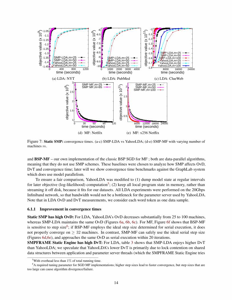
Figure 7: Static SMP: convergence times. (a-c) SMP-LDA vs YahooLDA; (d-e) SMP-MF with varying number ofmachines m.

and BSP-MF – our own implementation of the classic BSP SGD for MF ; both are data-parallel algorithms,meaning that they do not use SMP schemes. These baselines were chosen to analyze how SMP affects OvD,DvT and convergence time; later will we show convergence time benchmarks against the GraphLab systemwhich does use model parallelism.

To ensure a fair comparison, YahooLDA was modified to (1) dump model state at regular intervalsfor later objective (log-likelihood) computation5; (2) keep all local program state in memory, rather thanstreaming it off disk, because it fits for our datasets. All LDA experiments were performed on the 20GbpsInfiniband network, so that bandwidth would not be a bottleneck for the parameter server used by YahooLDA.Note that in LDA OvD and DvT measurements, we consider each word token as one data sample.

6.1.1 Improvement in convergence times

Static SMP has high OvD: For LDA, YahooLDA’s OvD decreases substantially from 25 to 100 machines,whereas SMP-LDA maintains the same OvD (Figures 6a, 6b, 6c). For MF, Figure 6f shows that BSP-MFis sensitive to step size6; if BSP-MF employs the ideal step size determined for serial execution, it doesnot properly converge on ≥ 32 machines. In contrast, SMP-MF can safely use the ideal serial step size(Figures 6d,6e), and approaches the same OvD as serial execution within 20 iterations.SMPFRAME Static Engine has high DvT: For LDA, table 3 shows that SMP-LDA enjoys higher DvTthan YahooLDA; we speculate that YahooLDA’s lower DvT is primarily due to lock contention on shareddata structures between application and parameter server threads (which the SMPFRAME Static Engine tries

5With overhead less than 1% of total running time.6A required tuning parameter for SGD MF implementations; higher step sizes lead to faster convergence, but step sizes that are

too large can cause algorithm divergence/failure.

14

Data set(size) #machines YahooLDA SMP-LDANYT(0.5GB) 25 38 43NYT(0.5GB) 50 79 62

PubMed(4.5GB) 25 38 60PubMed(4.5GB) 50 74 110ClueWeb(80GB) 25 39.7 58.3ClueWeb(80GB) 50 78 114ClueWeb(80GB) 100 151 204

Table 3: Static SMP: DvT for topic modeling (million tokens operated upon per second).

0

20

40

60

80

100

0 30 60 90

data

pro

cess

ed (

x 10

6 )

time (seconds)

Macro SyncMicro Sync

(a) DvT

-1.6

-1.55

-1.5

-1.45

-1.4

-1.35

-1.3

-1.25

-1.2

30 60 90

obje

ctiv

e va

lue

(x 1

09 )

time (seconds)

Macro SyncMicro Sync

(b) Time

-1.6

-1.55

-1.5

-1.45

-1.4

-1.35

-1.3

-1.25

-1.2

-1.15

0 300 600 900

obje

ctiv

e va

lue

(x 1

09 )

data processed (1M)

Macro SyncMicro Sync

(c) OvD

Figure 8: Static Engine: synchronization cost optimization. (a) macro synchronization improves DvT by 1.3 times;(b) it improves convergence speed by 1.3 times; (c) This synchronization strategy does not hurt OvD.

to avoid).Static SMP on SMPFRAME has low convergence times: Thanks to high OvD and DvT, SMP-LDA’sconvergence times are not only lower than YahooLDA, but also scale better with increasing machine count(Figures 7a, 7b, 7c). SMP-MF also exhibits good scalability (Figure 7d, 7e).

6.1.2 Benefits of Static Engine optimizations

The SMPFRAME Static Engine achieves high DvT (i.e iteration throughput) via two system optimizations:(1) reducing synchronization costs via the ring topology; (2) using a job pool to perform load balancingacross Job Executors.Reducing synchronization costs: Static SMP programs (including SMP-LDA and SMP-MF) do not requireall parameters to be synchronized across all machines, and this motivates the use of a ring topology. Forexample, consider SMP-LDA Algorithm 3: the word-rotation schedule() directly suggests that JobExecutors can pass parameters to their ring neighbor, rather than broadcasting to all machines; this appliesto SMP-MF as well.

SMPFRAME’s Static Engine implements this parameter-passing strategy via a ring topology, and onlyperforms a global synchronization barrier after all parameters have completed one rotation (i.e. P iterations)— we refer to this as “Macro Synchronization”. This has two effects: (1) network traffic becomes lessbursty, and (2) communication is effectively overlapped with computation; as a result, DvT is improvedby 30% compared to a naive implementation that invokes a synchronization barrier every iteration (“MicroSynchronization”, Figure 8a). This strategy does not negatively affect OvD (Figure 8c), and hence time toconvergence improves by about 30% (Figure 8b).Job pool load balancing: Uneven workloads are common in Static SMP programs: Figure 9a shows that theword distribution in LDA is highly skewed, meaning that some SMP-LDA update() jobs will be much

15

0.001

0.01

0.1

1

10

100

1000

0 30000 60000 90000

wor

d fr

eque

ncy

(x 1

03 )

rank

Word Frequency

(a) NYTimes

-1.6

-1.5

-1.4

-1.3

-1.2

-1.1

-1

40 80 120

obje

ctiv

e va

lue

(x 1

09 )

time (seconds)

load-balance enabledload-balance disabled

(b) Time

-1.6

-1.5

-1.4

-1.3

-1.2

-1.1

-1

0 200 400

obje

ctiv

e va

lue

(x 1

09 )

data processed (10M)

load-balance enabledload-balance disabled

(c) OvDFigure 9: Static Engine: Job pool load balancing. (a) Biased word frequency distribution in NYTimes data set; (b) bydispatching the 300 heaviest words first, convergence speed improves by 30 percent to reach objective value -1.02e+9;(c) this dispatching strategy does not hurt OvD.

longer than others. Hence, SMPFRAME dispatches the heaviest jobs first to the Job Executor threads. Thisimproves convergence times by 30% on SMP-LDA (Figure 9b), without affecting OvD.

6.1.3 Comparison against other systems:

We compare SMP-MF with GraphLab’s SGD MF implementation, on a different set of 8 machines — eachwith 64 cores, 128GB memory. On Netflix , GL-SGDMF converged to objective value 1.8e+8 in 300 seconds,and SMP-MF converged to 9.0e+7 in 302 seconds (i.e. better objective value in the same time). In terms ofDvT, SMP-MF touches 11.3m data samples per second, while GL-MF touches 4.5m data samples per second.

6.2 Dynamic SMP Scheduling

Our evaluation of dynamic-schedule SMP algoritms on the SMPFRAME Dynamic Engine shows significantlyimproved OvD compared to random model-parallel scheduling. We also show that (1) in the single machinesetting, Dynamic SMP comes at a cost to DvT, but overall convergence speed is still superior to randommodel-parallel; and (2) in the distributed setting, this DvT penalty mostly disappears.ML programs and baselines: We evaluate `1-regularized linear regression (Lasso) and `1-regularizedLogistic regression (sparse LR, or SLR) – SMPFRAME uses Algorithm 2 (SMP-Lasso) for the former,and we solve the latter using a minor modification to SMP-Lasso7 (called SMP-SLR). To the best ofour knowledge, there are no open-source distributed Lasso/SLR baselines that use coordinate descent, sowe implement the Shotgun Lasso/SLR algorithm [5] (Shotgun-Lasso, Shotgun-SLR), which uses randommodel-parallel scheduling8

6.2.1 Improvement in convergence times

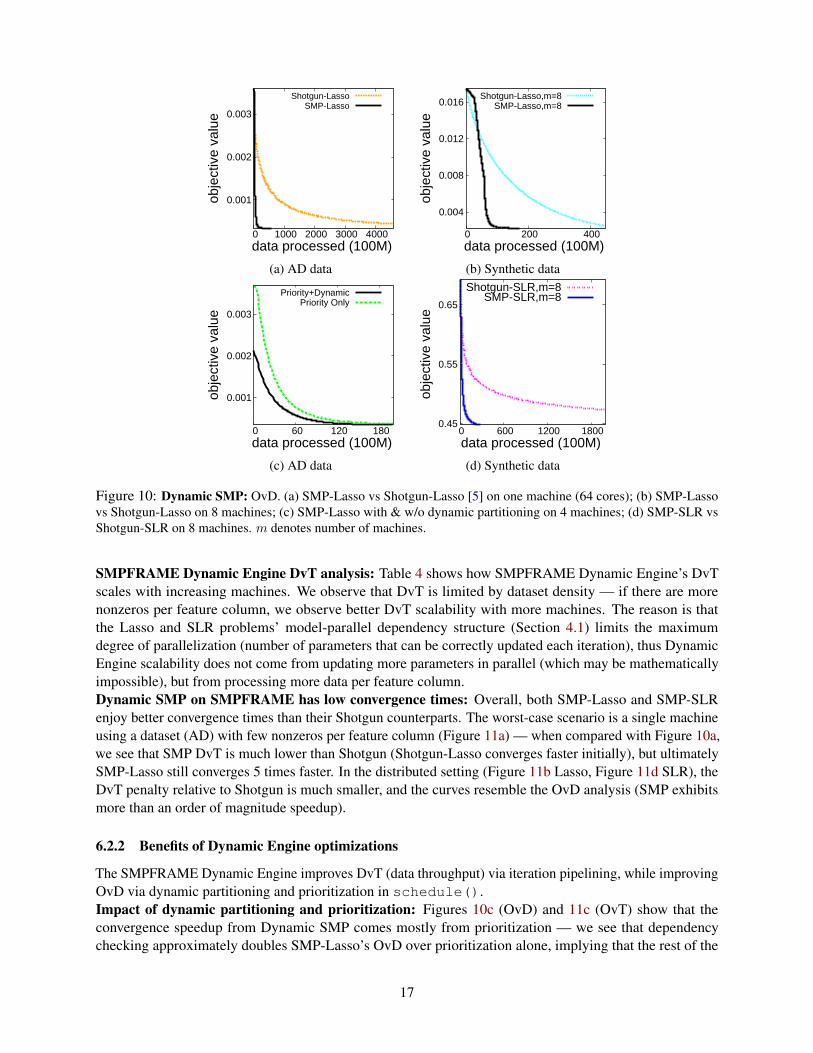
Dynamic SMP has high OvD: Dynamic SMP achieves high OvD, in both single-machine (Figure 10a) anddistributed, 8-machine (Figure 10b) configurations; here we have compared SMP-Lasso against randommodel-parallel Lasso (Shotgun-Lasso) [5]. In either case, Dynamic SMP decreases the data samples requiredfor convergence by an order of magnitude. Similar observations hold for distributed SMP-SLR versusShotgun-SLR (Figure 10d).

7Lasso and SLR are solved via the coordinate descent algorithm, hence SMP-Lasso and SMP-SLR only differ slightly intheir update equations. We use coordinate descent rather gradient descent because it has no step size tuning and more stableconvergence [25, 24].

8Using coordinate descent baselines is essential to properly evaluate the DvT and OvD impact of SMP-Lasso/SLR; otheralgorithms like stochastic gradient descent are only comparable in terms of convergence time.

16

0.001

0.002

0.003

0 1000 2000 3000 4000

obje

ctiv

e va

lue

data processed (100M)

Shotgun-LassoSMP-Lasso

(a) AD data

0.004

0.008

0.012

0.016

0 200 400

obje

ctiv

e va

lue

data processed (100M)

Shotgun-Lasso,m=8SMP-Lasso,m=8

(b) Synthetic data

0.001

0.002

0.003

0 60 120 180

obje

ctiv

e va

lue

data processed (100M)

Priority+DynamicPriority Only

(c) AD data

0.45

0.55

0.65

0 600 1200 1800ob

ject

ive

valu

e data processed (100M)

Shotgun-SLR,m=8SMP-SLR,m=8

(d) Synthetic data

Figure 10: Dynamic SMP: OvD. (a) SMP-Lasso vs Shotgun-Lasso [5] on one machine (64 cores); (b) SMP-Lassovs Shotgun-Lasso on 8 machines; (c) SMP-Lasso with & w/o dynamic partitioning on 4 machines; (d) SMP-SLR vsShotgun-SLR on 8 machines. m denotes number of machines.

SMPFRAME Dynamic Engine DvT analysis: Table 4 shows how SMPFRAME Dynamic Engine’s DvTscales with increasing machines. We observe that DvT is limited by dataset density — if there are morenonzeros per feature column, we observe better DvT scalability with more machines. The reason is thatthe Lasso and SLR problems’ model-parallel dependency structure (Section 4.1) limits the maximumdegree of parallelization (number of parameters that can be correctly updated each iteration), thus DynamicEngine scalability does not come from updating more parameters in parallel (which may be mathematicallyimpossible), but from processing more data per feature column.Dynamic SMP on SMPFRAME has low convergence times: Overall, both SMP-Lasso and SMP-SLRenjoy better convergence times than their Shotgun counterparts. The worst-case scenario is a single machineusing a dataset (AD) with few nonzeros per feature column (Figure 11a) — when compared with Figure 10a,we see that SMP DvT is much lower than Shotgun (Shotgun-Lasso converges faster initially), but ultimatelySMP-Lasso still converges 5 times faster. In the distributed setting (Figure 11b Lasso, Figure 11d SLR), theDvT penalty relative to Shotgun is much smaller, and the curves resemble the OvD analysis (SMP exhibitsmore than an order of magnitude speedup).

6.2.2 Benefits of Dynamic Engine optimizations

The SMPFRAME Dynamic Engine improves DvT (data throughput) via iteration pipelining, while improvingOvD via dynamic partitioning and prioritization in schedule().Impact of dynamic partitioning and prioritization: Figures 10c (OvD) and 11c (OvT) show that theconvergence speedup from Dynamic SMP comes mostly from prioritization — we see that dependencychecking approximately doubles SMP-Lasso’s OvD over prioritization alone, implying that the rest of the

17

0.001

0.002

0.003

0 400 800 1200 1600

obje

ctiv

e va

lue

time (seconds)

Shotgun-LassoSMP-Lasso

(a) AD data

0.004

0.008

0.012

0.016

0 2000 4000 6000 8000

obje

ctiv

e va

lue

time (seconds)

Shotgun-Lasso,m=8SMP-Lasso,m=8

(b) Synthetic data

0.001

0.002

0.003

0.004

60 120 180 240 300

obje

ctiv

e va

lue

time (seconds)

Priority+DynamicPriority Only

(c) AD data

0.45

0.55

0.65

0 3000 6000 9000ob

ject

ive

valu

e time (seconds)

Shotgun-SLR,m=8SMP-SLR,m=8

(d) Synthetic data

Figure 11: Dynamic SMP: convergence time. Subfigures (a-d) correspond to Figure 10.

aaaaaaaaaaApplication

nonzeros percolumn 1K 10K 20K

SMP-Lasso 16 × 4 cores 125 212 202SMP-Lasso 16 × 8 cores 162 306 344

SMP-LR 16 × 4 cores 75 98 103SMP-LR 16 × 8 cores 106 183 193

Table 4: Dynamic SMP: DvT of SMP-Lasso and SMP-LR, measured as data samples (millions) operated on persecond, for synthetic data sets with different column sparsity.

order-of-magnitude speedup over Shotgun-Lasso comes from prioritization. Additional evidence is providedby Figure 5; under prioritization most parameters converge within just 5 iterations.Pipelining improves DvT at a small cost to OvD: The SMPFRAME Dynamic Engine can pipeline iterationsto improve DvT (iteration throughput), at some cost to OvD. Figure 12c shows that SMP-Lasso (on 8machines) converges most quickly at a pipeline depth of 3, and Figure 12d provides a more detailedbreakdown, including the time take to reach the same objective value (0.0003). We make two observations:(1) DvT improvement saturates at pipeline depth 3; (2) OvD, expressed as the number of data samples toconvergence, gets proportionally worse as pipeline depth increases. Hence, the sweet spot for convergencetime is pipeline depth 3, which halves convergence time compared to no pipelining (depth 1).

6.2.3 Comparisons against other systems

We compare SMP-Lasso/SLR with Spark MLlib (Spark-Lasso, Spark-SLR), which uses the SGD algorithm.As with the earlier GraphLab comparison, we use 8 nodes with 64 cores and 128GB memory each. On the

18

0

300

600

900

1200

0 20 40 60

data

pro

cess

ed(1

0M)

time (seconds)

(a) DvT

0

0.001

0.002

0.003

0.004

0 800 1600 2400

obje

ctiv

e va

lue

data processed (10M)

Pipeline Depth 1 Pipeline Depth 2 Pipeline Depth 3 Pipeline Depth 4

(b) OvD

0.001

0.002

0.003

0.004

0 60 120 180

obje

ctiv

e va

lue

time (seconds)

Pipeline Depth 1 Pipeline Depth 2 Pipeline Depth 3 Pipeline Depth 4

(c) Time

0!

60!

120!

180!time (seconds)!

0!

80!

160!

240!

data processed (100M)!

0!

50!

100!

150!

200!

throughput !(1M/s) !

1 2 3 4! 1 2 3 4! 1 2 3 4!

(d) Metrics at objective 3e-4

Figure 12: Dynamic Engine: iteration pipelining. (a) DvT improves 2.5× at pipeline depth 3, however (b) OvDdecreases with increasing pipeline depth. Overall, (c) convergence time improves 2× at pipeline depth 3. (d) Anotherview of (a)-(c): we report DvT, OvD and time to converge to objective value 0.0003.

AD dataset (which has complex gene-gene correlations), Spark-Lasso reached objective value 0.0168 after 1hour, whereas SMP-Lasso achieved a lower objective (0.0003) in 3 minutes. On the LogisticSynthetic dataset(which was constructed to have few correlations), Spark-SLR converged to objective 0.452 in 899 seconds,while SMP-SLR achieved a similar result. This confirms that SMP is more effective in the presence of morecomplex model dependencies.

Finally, we want to highlight that the SMPFRAME system can significantly reduce the code requiredfor an SMP program: our SMP-Lasso implementation (Algorithm 2) has 390 lines in schedule(), 181lines in update() and aggregate(), and another 209 lines for miscellaneous uses like setting up theprogram environment; SMP-SLR uses a similar amount of code.

7 Related work

Early systems for scaling up ML focus on data parallelism [6] to leverage multi-core and multi-machinearchitecture, following the ideas in MapReduce [9]. Along these lines, Mahout[3] on Hadoop [2] and morerecently MLI [27] on Spark [35] have been developed.

The second generation of distributed ML systems — e.g. parameter servers (PS, [1, 8, 16, 20]) —address the problem of distributing large shared models across multiple workers. Early systems weredesigned for a particular class of ML problems, e.g., [1] for LDA and [8] for deep neural nets. More recentwork [16, 20] have generalized the parameter server concept to support a wide range of ML algorithms.There are counterparts to parameter server ideas in SMPFRAME: for instance, stale synchronous parallel(SSP, [16, 7]) and SMPFRAME both control parameter staleness; the former through bookkeeping on thedeviation between workers, and the latter through pipeline depth. Another example is filtering [20], which

19

resembles parameter scheduling in SMPFRAME, but is primarily for alleviating synchronization costs, e.g.,their KKT filter suppresses transmission of “unnecessary” gradients, while SMPFRAME goes a step furtherand uses algorithm information to make update choices (not just synchronization choices).

None of the above systems directly address the issue of conflict updates, which leads to slow convergenceor even algorithmic failure. Within the parallel ML literature, dependency checking is either performed case-by-case [12, 33]; or simply ignored [5, 23]. The first systematic approach was proposed by GraphLab [21, 13],where ML computational dependencies are encoded by the user in a graph, so that the system may selectdisjoint subgraphs to process in parallel — thus, graph-scheduled model parallel ML algorithms can be writtenin GraphLab. Intriguing recent work, GraphX [14], combines these sophisticated GraphLab optimizationswith database-style data processing and runs on a BSP-style MapReduce framework, sometimes withoutsignificant loss of performance.

Task prioritization (to exploit uneven convergence of iterative algorithms) was studied by PrIter [37] andGraphLab [21]. The former, built on Hadoop [2], prioritizes data points that contribute most to convergence,while GraphLab ties prioritization to the program’s graph representation. SMPFRAME prioritizes the mostpromising model parameter values.

8 Conclusion

We developed SMPFRAME to improve the convergence speed of model-parallel ML at scale, achieving bothhigh progress per iteration (via dependency checking and prioritization through SMP programming), andhigh iteration throughput (via SMPFRAME system optimizations such as pipelining and the ring topology).Consequently, SMP programs running on SMPFRAME achieve a marked performance improvement overrecent, well-established baselines: to give two examples, SMP-LDA converges 10x faster than YahooLDA,while SMP-Lasso converges 5x faster than randomly-scheduled Shotgun-Lasso.

There are some issues that we would like to address in future: chief amongst them is automaticschedule() creation; ideally users should only have to implement update() and aggregate(),while leaving scheduling to the system. Another issue is generalizability and programmability — whatother ML programs might benefit from SMP, and can we write them easily? Finally, using a different solveralgorithm (e.g. Alternating Least Squares or Cyclic Coordinate Descent instead of SGD) can sometimesspeed up an ML application; SMPFRAME supports such alternatives, though their study is beyond the scopeof this work.

20

References

[1] AHMED, A., ALY, M., GONZALEZ, J., NARAYANAMURTHY, S., AND SMOLA, A. J. Scalableinference in latent variable models. In WSDM (2012).

[2] Apache Hadoop, http://hadoop.apache.org.

[3] Apache Mahout, http://mahout.apache.org.

[4] BLEI, D. M., NG, A. Y., AND JORDAN, M. I. Latent Dirichlet allocation. Journal of MachineLearning Research 3 (2003), 993–1022.

[5] BRADLEY, J. K., KYROLA, A., BICKSON, D., AND GUESTRIN, C. Parallel coordinate descent forl1-regularized loss minimization. In ICML (2011).

[6] CHU, C., KIM, S. K., LIN, Y.-A., YU, Y., BRADSKI, G., NG, A. Y., AND OLUKOTUN, K. Map-reduce for machine learning on multicore. NIPS (2007).

[7] DAI, W., KUMAR, A., WEI, J., HO, Q., GIBSON, G. A., AND XING, E. P. High-performancedistributed ML at scale through parameter server consistency models. In AAAI (2015).

[8] DEAN, J., CORRADO, G., MONGA, R., CHEN, K., DEVIN, M., MAO, M., AURELIO RANZATO,M., SENIOR, A., TUCKER, P., YANG, K., LE, Q. V., AND NG, A. Y. Large scale distributed deepnetworks. In NIPS. 2012.

[9] DEAN, J., AND GHEMAWAT, S. MapReduce: simplified data processing on large clusters. Communica-tions of the ACM 51, 1 (2008), 107–113.

[10] FRIEDMAN, J., HASTIE, T., HOFLING, H., AND TIBSHIRANI, R. Pathwise coordinate optimization.Annals of Applied Statistics 1, 2 (2007), 302–332.

[11] FU, W. Penalized regressions: the bridge versus the lasso. Journal of Computational and GraphicalStatistics 7, 3 (1998), 397–416.

[12] GEMULLA, R., NIJKAMP, E., HAAS, P. J., AND SISMANIS, Y. Large-scale matrix factorization withdistributed stochastic gradient descent. In KDD (2011).

[13] GONZALEZ, J. E., LOW, Y., GU, H., BICKSON, D., AND GUESTRIN, C. Powergraph: Distributedgraph-parallel computation on natural graphs. In OSDI (2012), vol. 12, p. 2.

[14] GONZALEZ, J. E., XIN, R. S., DAVE, A., CRANKSHAW, D., FRANKLIN, M. J., AND STOICA, I.Graphx: Graph processing in a distributed dataflow framework. In Proceedings of the 11th USENIXSymposium on Operating Systems Design and Implementation (OSDI) (2014).

[15] GRIFFITHS, T. L., AND STEYVERS, M. Finding scientific topics. Proceedings of National Academy ofScience 101 (2004), 5228–5235.

[16] HO, Q., CIPAR, J., CUI, H., LEE, S., KIM, J. K., GIBBONS, P. B., GIBSON, G. A., GANGER, G. R.,AND XING, E. P. More effective distributed ML via a stale synchronous parallel parameter server. InNIPS (2013).

[17] KARYPIS, G., AND KUMAR, V. Metis-unstructured graph partitioning and sparse matrix orderingsystem, version 2.0.

[18] KRIZHEVSKY, A., SUTSKEVER, I., AND HINTON, G. E. Imagenet classification with deep convolu-tional neural networks. In NIPS (2012).

[19] LEE, S., KIM, J. K., ZHENG, X., HO, Q., GIBSON, G., AND XING, E. P. On model parallelism andscheduling strategies for distributed machine learning. In NIPS. 2014.

[20] LI, M., ANDERSEN, D. G., PARK, J. W., SMOLA, A. J., AHMED, A., JOSIFOVSKI, V., LONG, J.,SHEKITA, E. J., AND SU, B.-Y. Scaling distributed machine learning with the parameter server. InOSDI (2014).

[21] LOW, Y., BICKSON, D., GONZALEZ, J., GUESTRIN, C., KYROLA, A., AND HELLERSTEIN, J. M.Distributed graphlab: A framework for machine learning and data mining in the cloud. Proc. VLDBEndow. 5, 8 (2012), 716–727.

[22] POWER, R., AND LI, J. Piccolo: Building fast, distributed programs with partitioned tables. In OSDI(2010).

[23] RECHT, B., RE, C., WRIGHT, S., AND NIU, F. Hogwild: A lock-free approach to parallelizingstochastic gradient descent. In NIPS (2011).

[24] RICHTARIK, P., AND TAKAC, M. Parallel coordinate descent methods for big data optimization. arXivpreprint arXiv:1212.0873 (2012).

[25] SCHERRER, C., HALAPPANAVAR, M., TEWARI, A., AND HAGLIN, D. Scaling up parallel coordinatedescent algorithms. In ICML (2012).

[26] SCHERRER, C., TEWARI, A., HALAPPANAVAR, M., AND HAGLIN, D. Feature clustering foraccelerating parallel coordinate descent. In NIPS. 2012.

[27] SPARKS, E. R., TALWALKAR, A., SMITH, V., KOTTALAM, J., PAN, X., GONZALEZ, J., FRANKLIN,M. J., JORDAN, M. I., AND KRASKA, T. MLI: An API for distributed machine learning. In ICDM(2013).

[28] TIBSHIRANI, R. Regression shrinkage and selection via the lasso. Journal of the Royal StatisticalSociety. Series B (Methodological) 58, 1 (1996), 267–288.

[29] TIERNEY, L. Markov chains for exploring posterior distributions. the Annals of Statistics (1994),1701–1728.

[30] WANG, M., XIAO, T., LI, J., ZHANG, J., HONG, C., AND ZHANG, Z. Minerva: A scalable and highlyefficient training platform for deep learning.

[31] WANG, Y., ZHAO, X., SUN, Z., YAN, H., WANG, L., JIN, Z., WANG, L., GAO, Y., LAW, C., AND

ZENG, J. Peacock: Learning long-tail topic features for industrial applications. ACM Transactions onIntelligent Systems and Technology 9, 4 (2014).

[32] YAO, L., MIMNO, D., AND MCCALLUM, A. Efficient methods for topic model inference on streamingdocument collections. In KDD (2009).

[33] YUAN, J., GAO, F., HO, Q., DAI, W., WEI, J., ZHENG, X., XING, E. P., LIU, T.-Y., AND MA,W.-Y. LightLDA: Big topic models on modest compute clusters. In WWW (2015).

[34] ZAHARIA, M., CHOWDHURY, M., DAS, T., DAVE, A., MA, J., MCCAULEY, M., FRANKLIN, M. J.,SHENKER, S., AND STOICA, I. Resilient distributed datasets: a fault-tolerant abstraction for in-memorycluster computing. In NSDI (2012).

[35] ZAHARIA, M., DAS, T., LI, H., HUNTER, T., SHENKER, S., AND STOICA, I. Discretized streams:Fault-tolerant streaming computation at scale. In Proceedings of the Twenty-Fourth ACM Symposiumon Operating Systems Principles (New York, NY, USA, 2013), SOSP ’13, ACM, pp. 423–438.

[36] ZHANG, B., GAITERI, C., BODEA, L.-G., WANG, Z., MCELWEE, J., PODTELEZHNIKOV, A. A.,ZHANG, C., XIE, T., TRAN, L., DOBRIN, R., ET AL. Integrated systems approach identifies geneticnodes and networks in late-onset Alzheimer’s disease. Cell 153, 3 (2013), 707–720.

[37] ZHANG, Y., GAO, Q., GAO, L., AND WANG, C. Priter: A distributed framework for prioritizediterative computations. In SOCC (2011).

[38] ZINKEVICH, M., WEIMER, M., LI, L., AND SMOLA, A. J. Parallelized stochastic gradient descent.In NIPS (2010).