Social Game for Building Energy Efficiency: UtilityLearning, Simulation, Analysis and Incentive Design

Ioannis KonstantakopoulosCostas J. SpanosS. Shankar Sastry

Electrical Engineering and Computer SciencesUniversity of California at Berkeley

Technical Report No. UCB/EECS-2015-3http://www.eecs.berkeley.edu/Pubs/TechRpts/2015/EECS-2015-3.html

February 2, 2015

Copyright © 2015, by the author(s).All rights reserved.

Permission to make digital or hard copies of all or part of this work forpersonal or classroom use is granted without fee provided that copies arenot made or distributed for profit or commercial advantage and thatcopies bear this notice and the full citation on the first page. To copyotherwise, to republish, to post on servers or to redistribute to lists,requires prior specific permission.

Acknowledgement

Firstly, I would like to thank my advisor, Professor Spanos Costas forsupporting my research, accepting me into his research group andproviding me advice and kind encouragement. In addition, I want tothank Professor Shankar Sastry for his help and support. Also, I feelindebted to my collaborators Ming Jin and Lillian Ratliff for their kindlyhelp during my research. Moreover, I am grateful to Kakali Georgia forher valuable support, help and love all these years as well as my familyfor their love. Finally, the present work was partially financially supportedby the "Andreas Mentzelopoulos Scholarships University of Patras".

Social Game for Building Energy Efficiency: Utility Learning, Simulation,

Analysis and Incentive Design

by Konstantakopoulos Ioannis

Research Project

Submitted to the Department of Electrical Engineering and Computer Sciences, University of

California at Berkeley, in partial satisfaction of the requirements for the degree of Master of Sci-

ence, Plan II.

Approval for the Report and Comprehensive Examination:

Committee:

Professor Costas J. Spanos

Research Advisor

Date

* * * * * *

Second Reader’s Name

Professor S. Shankar Sastry

Date

Contents

List of Figures . . . . . . . . . . . . . . . . . . . . . . . . . . . . . . . . . . . . . . . . . . . . i

List of Tables . . . . . . . . . . . . . . . . . . . . . . . . . . . . . . . . . . . . . . . . . . . . . iii

Acknowledgment . . . . . . . . . . . . . . . . . . . . . . . . . . . . . . . . . . . . . . . . . . vi

Abstract . . . . . . . . . . . . . . . . . . . . . . . . . . . . . . . . . . . . . . . . . . . . . . . . vii

1 Introduction 1

1.1 Thesis Organization . . . . . . . . . . . . . . . . . . . . . . . . . . . . . . . . . . . . . 4

2 Experimental Setup 5

2.1 Social Game Web portal . . . . . . . . . . . . . . . . . . . . . . . . . . . . . . . . . . . 5

2.2 App Design . . . . . . . . . . . . . . . . . . . . . . . . . . . . . . . . . . . . . . . . . . . 9

2.2.1 Environment Specifics . . . . . . . . . . . . . . . . . . . . . . . . . . . . . . . . 10

2.2.2 Model-View-Controller (MVC) . . . . . . . . . . . . . . . . . . . . . . . . . . . 10

2.2.3 App design outline . . . . . . . . . . . . . . . . . . . . . . . . . . . . . . . . . . 12

2.2.4 Use-case scenario . . . . . . . . . . . . . . . . . . . . . . . . . . . . . . . . . . . 13

2

2.2.5 Future improvements . . . . . . . . . . . . . . . . . . . . . . . . . . . . . . . . 14

3 Game Formulation 18

3.1 Follower Game . . . . . . . . . . . . . . . . . . . . . . . . . . . . . . . . . . . . . . . . 19

3.2 Leader Optimization Problem – Incentive Design . . . . . . . . . . . . . . . . . . . . 24

4 Utility Estimation 28

5 Results 31

5.1 Utility estimations - Energy savings . . . . . . . . . . . . . . . . . . . . . . . . . . . . 31

5.1.1 Savings . . . . . . . . . . . . . . . . . . . . . . . . . . . . . . . . . . . . . . . . . 32

5.1.2 Estimation . . . . . . . . . . . . . . . . . . . . . . . . . . . . . . . . . . . . . . . 34

5.1.3 Simulation . . . . . . . . . . . . . . . . . . . . . . . . . . . . . . . . . . . . . . . 36

5.2 Incentive Design . . . . . . . . . . . . . . . . . . . . . . . . . . . . . . . . . . . . . . . 37

6 Conclusions 44

6.1 Summary . . . . . . . . . . . . . . . . . . . . . . . . . . . . . . . . . . . . . . . . . . . . 44

6.2 Future Work . . . . . . . . . . . . . . . . . . . . . . . . . . . . . . . . . . . . . . . . . . 45

List of symbols 47

Bibliography 48

List of Figures

2.1 Lighting and HVAC zones of the office . . . . . . . . . . . . . . . . . . . . . . . . . . 6

2.2 Power Line Chart for individual with id number 17 . . . . . . . . . . . . . . . . . . . 7

2.3 Live map view of the office for the shared energy sources . . . . . . . . . . . . . . . 8

2.4 Power Line Chart for individual with id number 17 . . . . . . . . . . . . . . . . . . . 9

2.5 Live map view of the office for the shared energy sources . . . . . . . . . . . . . . . 10

2.6 Display of an occupant’s point balance and a chart of his / her points balance com-

pared with other occupants’ point balance . . . . . . . . . . . . . . . . . . . . . . . . 11

2.7 Live map view of the office for the shared energy sources . . . . . . . . . . . . . . . 12

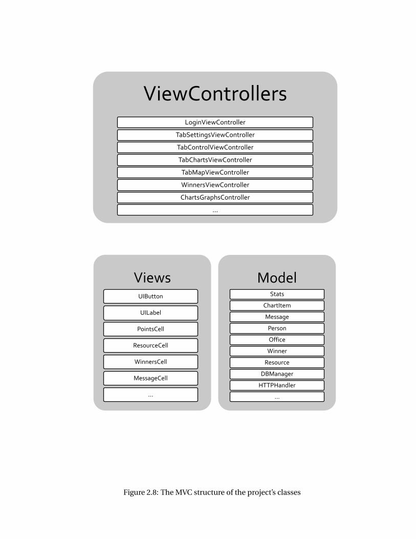
2.8 The MVC structure of the project’s classes . . . . . . . . . . . . . . . . . . . . . . . . 15

2.9 Left: The home tab - providing user info and announcements. Right: the user

points and statistics . . . . . . . . . . . . . . . . . . . . . . . . . . . . . . . . . . . . . . 16

2.10 Left: The laboratory’s map - providing users’ votes and energy status Right: the

user available resources and controls . . . . . . . . . . . . . . . . . . . . . . . . . . . 17

3.1 Human utility behavior . . . . . . . . . . . . . . . . . . . . . . . . . . . . . . . . . . . 21

ii

5.1 Lights’ average daily dim level . . . . . . . . . . . . . . . . . . . . . . . . . . . . . . . 32

5.2 Lights’ daily total energy consumption . . . . . . . . . . . . . . . . . . . . . . . . . . 33

5.3 Actual implemented temperature levels in the two zones of the office building . . . 34

5.4 User 8 light histogram of estimation of θi in the default region 20 . . . . . . . . . . . 35

5.5 User 14 light histogram of estimation of θi in the default region 20 . . . . . . . . . . 35

5.6 Estimation of average daily light votes . . . . . . . . . . . . . . . . . . . . . . . . . . . 37

5.7 Estimation of average daily HVAC votes . . . . . . . . . . . . . . . . . . . . . . . . . . 38

5.8 Energy consumption data for the Lutron lighting system in kWh as a function of

the lighting setting. . . . . . . . . . . . . . . . . . . . . . . . . . . . . . . . . . . . . . . 39

5.9 Utility of occupant 2 as a function of (d ,ρ) at the mean Nash equilibrium after

running 1000 simulations. Notice that for fixed values of d the utility value is near

constant in ρ. Also, occupant 2 has very large utility when the default setting is

around 70. . . . . . . . . . . . . . . . . . . . . . . . . . . . . . . . . . . . . . . . . . . . 40

5.10 Mean of the Nash equilibria of the simulated games over 103 days under estimated

occupant utilities with leader incentives found via PSO and parameters given by

(d ,ρ,β2,∑

j∈Aβ j ) where A = 6,8,14,20. Note that the mean Nash equilibrium in

each case is slightly below the default setting. . . . . . . . . . . . . . . . . . . . . . . 43

List of Tables

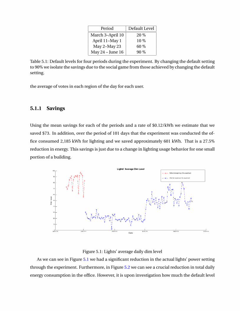
5.1 Default levels for four periods during the experiment. By changing the default

setting to 90% we isolate the savings due to the social game from those achieved

by changing the default setting. . . . . . . . . . . . . . . . . . . . . . . . . . . . . . . . 32

5.2 Estimated lighting utility parameter for selected set of active users for the daily

average vote. The standard deviation is indicated inside the parentheses and the

mean is given outside of the parentheses. . . . . . . . . . . . . . . . . . . . . . . . . . 36

5.3 Estimated HVAC utility parameter for selected set of active users for the daily aver-

age vote. The standard deviation is indicated inside the parentheses and the mean

is given outside of the parentheses. . . . . . . . . . . . . . . . . . . . . . . . . . . . . 36

5.4 Leader’s utility in dollars for the values (d∗,ρ∗,β2,∑

j∈Aβ j ) where β2 is the benev-

olence factor for user 2 and 1−β2 =∑j∈Aβ j is the sum of the benevolence factors

for the occupants A = 6,8,14,20. The utility value is determined by solving the

leader’s optimization problem using the PSO method and simulating the occupant

game via the dynamical system given in (22). The value of the utility is interpreted

as the energy saved in dollars by the leader plus the utility as measured in dollars.

We use a rate of $0.12 per kWh. . . . . . . . . . . . . . . . . . . . . . . . . . . . . . . . 41

iv

5.5 Leader’s utility in dollars for the previously implemented (d ,ρ) for various benev-

olence factors β= (β2,∑

j∈Aβ j ) where A = 6,8,14,20. The value is interpreted as

the energy saved in dollars by the leader plus the utility as measured in dollars. We

use a rate of $0.12 per kWh as this is the approximate rate charged by the buildings

on the UC Berkeley campus. . . . . . . . . . . . . . . . . . . . . . . . . . . . . . . . . 41

Acknowledgment

Firstly, I would like to thank my advisor, Professor Spanos Costas for supporting my research,

accepting me into his research group and providing me advice and kind encouragement. In ad-

dition, I want to thank Professor Shankar Sastry for his help and support. Also, I feel indebted to

my collaborators Ming Jin and Lillian Ratliff for their kindly help during my research. Moreover,

I am grateful to Kakali Georgia for her valuable support, help and love all these years as well

as my family for their love. Finally, the present work was partially financially supported by the

"Andreas Mentzelopoulos Scholarships University of Patras".

Abstract

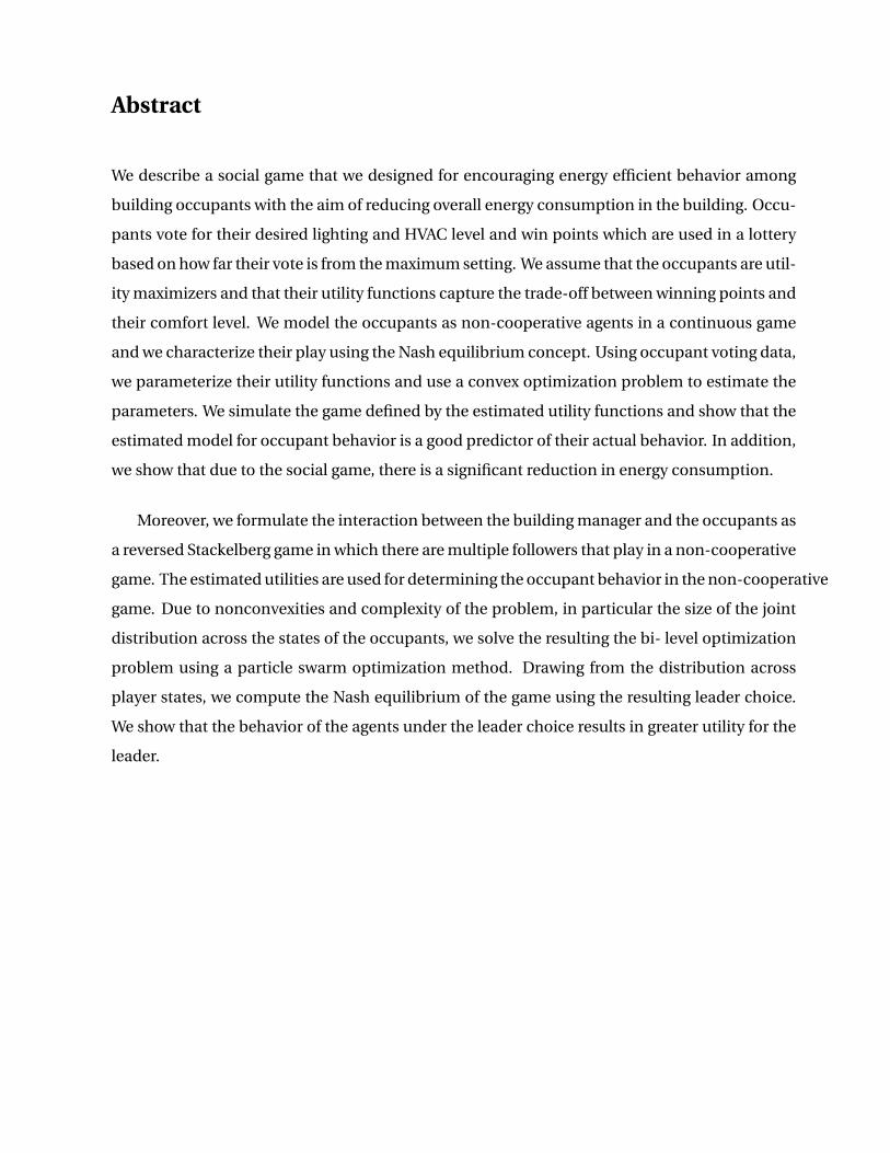
We describe a social game that we designed for encouraging energy efficient behavior among

building occupants with the aim of reducing overall energy consumption in the building. Occu-

pants vote for their desired lighting and HVAC level and win points which are used in a lottery

based on how far their vote is from the maximum setting. We assume that the occupants are util-

ity maximizers and that their utility functions capture the trade-off between winning points and

their comfort level. We model the occupants as non-cooperative agents in a continuous game

and we characterize their play using the Nash equilibrium concept. Using occupant voting data,

we parameterize their utility functions and use a convex optimization problem to estimate the

parameters. We simulate the game defined by the estimated utility functions and show that the

estimated model for occupant behavior is a good predictor of their actual behavior. In addition,

we show that due to the social game, there is a significant reduction in energy consumption.

Moreover, we formulate the interaction between the building manager and the occupants as

a reversed Stackelberg game in which there are multiple followers that play in a non-cooperative

game. The estimated utilities are used for determining the occupant behavior in the non-cooperative

game. Due to nonconvexities and complexity of the problem, in particular the size of the joint

distribution across the states of the occupants, we solve the resulting the bi- level optimization

problem using a particle swarm optimization method. Drawing from the distribution across

player states, we compute the Nash equilibrium of the game using the resulting leader choice.

We show that the behavior of the agents under the leader choice results in greater utility for the

leader.

Chapter 1

Introduction

Energy consumption of buildings, both residential and commercial, accounts for approximately

40% of all energy usage in the U.S. [18]. Lighting is a major consumer of energy in commercial

buildings; one-fifth of all energy consumed in buildings is due to lighting [26]. There have been

many approaches to improve energy efficiency of buildings through control and automation as

well as incentives and pricing. From the meter to the consumer, many control methods, such as

model predictive control, have been proposed as a means to improve the efficiency of building

operations (see, e.g., [2, 5, 6, 15, 20, 14]). From the meter to the energy utility, many economic

solutions have been proposed, such as dynamic pricing and mechanisms including incentives,

rebates, and recommendations, to reduce consumption (see, e.g., [16],[24]).

Many of the past approaches to building energy management only focus on heating and

cooling of the building [Model Predictive Control]. We are advocating that due to new tech-

nological advances in building automation, incentives can be designed around more than just

heating, ventilation and air conditioning (HVAC) systems. In particular, our experimental set-up

allows us to design incentives based on lighting and individual plug-load in addition to HVAC.

In the set-up, the building manager interacts with occupants through a social game. Started

from the Spring 2014 an experiment is conducted in the Center for Research in Energy Systems

Transformation (CREST) at the University of California, Berkeley.

Actually, the experiment tries to investigate the effects of incentives on the overall energy

1

consumption, as well as patterns of energy usage by occupants of a floor of an office building.

The incentives were incorporated into a social game, which rewarded individual users for saving

energy. Social games have been used to alleviate congestion in transportation systems [19] as

well as in the healthcare domain for understanding the tradeoff between privacy and desire to

win by expending calories [4].

It is essential for the building energy management to understand possible patterns of the

occupants like their thermal comfort level, their light preferences, their daily schedule to men-

tion but a few. This is an advantage of an application of our social game due to the fact that

can derive vital data and occupants’ patterns. All these data can be used for an energy efficient

automatic control of the office building (lighting and HVAC control).

There are many ways in which a building manager can be motivated to encourage energy ef-

ficient behavior. The most obvious is that they pay the bill or, due to some operational excellence

measure, are required to maintain an energy efficient building. Beyond these motivations, re-

cently demand response programs are being implemented by utility companies with the goal of

correcting for improper load forecasting (see, e.g., [1],[17], [13]). In such a program, consumers

enter into a contract with the utility company in which they agree to change their demand in

accordance with some agreed upon schedule. In this scenario, the building manager may now

be required to keep this schedule.

Our approach to efficient building energy management focuses on office buildings and uti-

lizes new building automation products such as the Lutron lighting system1. We design a social

game aimed at incentivizing occupants to modify their behavior so that the overall energy con-

sumption in the building is reduced. The social game consists of occupants logging their vote

for the lighting setting in the office. They win points based on how energy efficient their vote is

compared to other occupants. After each vote is logged, the average of the votes is implemented

in the office. The points are used to determine an occupant’s likelihood of winning in a lottery.

We designed an online platform so that occupants can log in and vote, view their points,

and observe all occupants’ consumption patterns and points. This platform also stores all the

past data allowing us to use it for estimating occupant behavior and compute online different

1http://www.lutron.com/en-US/Pages/default.aspx

possible incentives. Moreover, we have recently designed a smartphone app so as the users

to view their account’s details with a more efficient way as well as to vote for their light and

temperature preferences. Our next step is the design of an app for tablets, which will give to the

occupants a more convenient way of accessing our platform.

We modeled the occupants as non- cooperative agents who achieve a Nash equilibrium

point. Under this assumption, we were able to use necessary and sufficient first and second

order conditions [21] to cast the utility estimation problem as a convex optimization problem

in the parameters of the occupants’ utility functions. We showed that estimating agent utility

functions via this method results in a predictive model that out performs several other standard

techniques. Furthermore, we showed that based on the estimations of the occupants’ utility

functions and the past data, we can forecast the building’s light / temperature level with small

mean square error. For this task, we tried different online techniques so as to use the past data

efficiently.

We are able to leverage the fact that we modeled the occupants as utility maximers in a game-

theoretic framework in the formulation of the building manager’s problem as a reversed Stack-

elberg game. A major advantage of modeling occupants as utility maximizers competing in a

game and using the Nash equilibrium concept is this game theoretic model fits in the Stack-

elberg framework for incentive design in which the building manager performs an online esti-

mation of occupant’s utility function and designs incentives for behavior modification. This, in

essence, is a problem of closing- the-loop around the occupants so that the building manager

achieves sustained energy savings.

In particular, we formulate the building manager’s optimization problem as a bi-level opti-

mization problem in which the inner optimization problem is a non-cooperative game between

the occupants and the outer optimization problem is the maximization of the building man-

ager’s utility over the total points and default lighting setting.

Given the data from our social game experiment, we estimate the occupants’ utility func-

tions. We determine a distribution for each occupant over the set of events, which include the

occupant states present and active, present and remaining at the default, and absent. We refer

to these as the player states and shorten them to active, default, and absent. Due to the number

of events in the joint distribution across possible occupant states, we employ a particle swarm

optimization method for solving the building manager’s bi- level optimization problem for the

total points and default lighting setting. This results in a suboptimal solution; however, we show

that the solution leads to an occupant’s behavior that results in a larger utility for the building

manager as compared to previously implemented schemes.

1.1 Thesis Organization

The rest of this thesis is organized as follows. We begin in Chapter 2 by describing the exper-

imental setup for our social game test-bed. In Chapter 3, we present the game formulation.

There are games at two levels; the inner non- cooperative continuous game between the occu-

pants and the outer reversed Stackelberg game between the building manager and the followers.

Moreover, we describe the utility estimation and incentive design (solution to the building man-

ager’s optimization problem) in Chapter 4. We continue with the results and the discussion at

Chapter 5. Finally, in Chapter 6, we offer some concluding remarks and directions for future

work.

Chapter 2

Experimental Setup

2.1 Social Game Web portal

The social game for energy savings that we have designed is such that occupants in an office

building vote according to their usage preferences of shared resources and are rewarded with

points based on how energy efficient their strategy is in comparison with the other occupants.

Having points increases the likelihood of the occupant winning in a lottery every week. The

prizes in the lottery consist of three Amazon gift cards.

As it was mentioned in the introduction, we have installed a Lutron1 system for the control

of the lights and the HVAC system in the office. This system allows us to precisely control the

lighting level (the lights are dimmable) of each of the lights in the office as well as to the HVAC

temperature set point. We use it to set the default lighting and HVAC level as well as implement

the average of the votes each time the occupants change their lighting and/or HVAC preferences.

It is vital to mention that the change of the lighting level is instantaneous and for the HVAC there

is a delay of 5 up to 10 minutes.

We have divided the office into five lighting zones and each zone has four occupants. Thus,

there are 20 occupants who participate in the social game. In addition, we have two heating,

1http://www.lutron.com/en-US/Pages/default.aspx

5

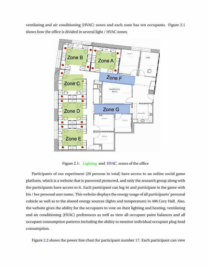
ventilating and air conditioning (HVAC) zones and each zone has ten occupants. Figure 2.1

shows how the office is divided in several light / HVAC zones.

1.4 Games’ Interface / Web Portal Participants of our experiment (20 persons in total) have access to an online social game platform, which is a website that is password protected, and only the research group along with the participants have access to it. Each participant has a personal username in order to login to the web portal. This website, display the energy usage of all participants as well as to the shared energy sources light and temperature levels in 406 Cory Hall. Also, the website gives to each participant information about his / her total points along with instantaneous control of the shared lights / temperature. Below there are figures that show the web portal of our experiment.

Figure 1: Map view of the office along with the light / temperature zones

Figure 2.1: Lighting and HVAC zones of the office

Participants of our experiment (20 persons in total) have access to an online social game

platform, which is a website that is password protected, and only the research group along with

the participants have access to it. Each participant can log-in and participate in the game with

his / her personal user name. This website displays the energy usage of all participants’ personal

cubicle as well as to the shared energy sources (lights and temperature) in 406 Cory Hall. Also,

the website gives the ability for the occupants to vote on their lighting and heating, ventilating

and air conditioning (HVAC) preferences as well as view all occupant point balances and all

occupant consumption patterns including the ability to monitor individual occupant plug-load

consumption.

Figure 2.2 shows the power line chart for participant number 17. Each participant can view

his / her power line chart in addition to the power line chart of other participants. For example,

as we can see from the figure 2.2 participant with id number 17 turn of his / her plug-load at the

night before he / she leaves. Therefore, a future part of the social game is to try to motivate the

occupants to turn off their plug-load before they leave as well as to understand their working

patterns and try to apply an automatic way of controlling the plug-load energy consumption.

Moreover, the participants of the experiment can view lively the conditions on the office. In

that way, they are able to vote based on the conditions (shared lights and HVAC level) as well

as to their own comfort level. Figure 2.3 shows the page of our web portal that shows lively the

level of the shared sources. It is actually a weight between the conditions at the office and their

comfort level to the optimal vote so as they to have maximum likelihood of winning the lottery

prices. So, they are able to see the light level of the office area as well as above their desk. In

addition, they can view the temperature in the office.

Figure 2.2: Power Line Chart for individual with id number 17

Furthermore, the participants have access in past data through the web site. So, they can

view their own votes as well as the light / HVAC conditions of the office for several past dates of

their choice. Figure 2.4 shows the light chart of light zones A and B in addition to participant’s

with id number 2 votes. Also, Figure 2.5 shows HVAC chart of temperature zones A and B in

addition to participant’s with id number 2 votes.

Figure 2.7 shows the actual page in our web portal at which the occupants can vote for their

lighting and heating, ventilating and air conditioning (HVAC) preferences. Also, figure 2.6 shows

Figure 2.3: Live map view of the office for the shared energy sources

a sample of how occupants can see their point balance as well as how their points are in com-

parison to the other occupant’s point balance.

We try to find the optimal way so as to design a game focused on encouraging occupants to

select lower lighting settings in exchange for a chance to win in a lottery. An occupant’s vote is

for the lighting level in their zone as well as for neighboring zones. The lighting setting that is

implemented is the average of all the votes.

Each day when an occupant logs into the online platform the first time after they enter the

office, they are considered present for the remainder of the day. Upon logging in the web-portal

the occupants can log their votes, view their point balance as well as other occupants’ points,

and view all occupants past consumption patterns. If they actively change their vote from the

default to some other value, then we consider them active. On the other hand, if they choose

not to change their vote from the default setting, then they are considered default for the day. If

they do not enter the office on a given day, then they are considered absent.

There is a default lighting setting. An occupant can leave the lighting setting as the default

after logging in or they can change it to some other value in the interval [0,100] ([70,78]) for the

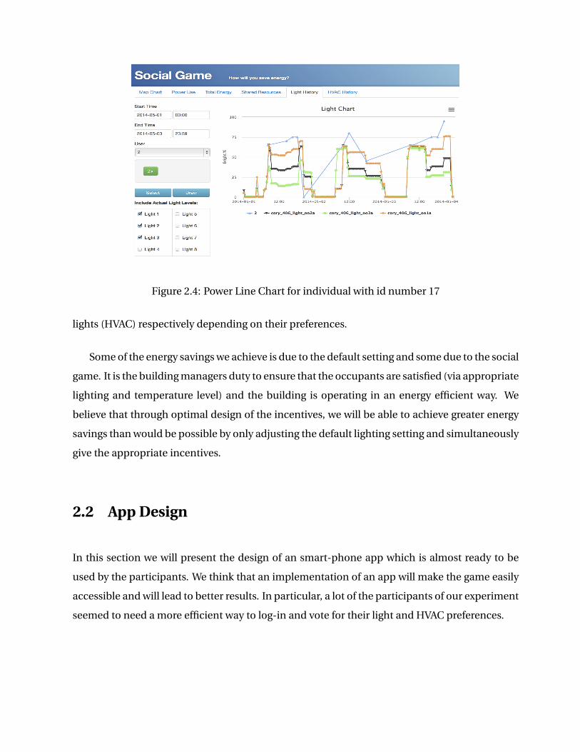
Figure 2.4: Power Line Chart for individual with id number 17

lights (HVAC) respectively depending on their preferences.

Some of the energy savings we achieve is due to the default setting and some due to the social

game. It is the building managers duty to ensure that the occupants are satisfied (via appropriate

lighting and temperature level) and the building is operating in an energy efficient way. We

believe that through optimal design of the incentives, we will be able to achieve greater energy

savings than would be possible by only adjusting the default lighting setting and simultaneously

give the appropriate incentives.

2.2 App Design

In this section we will present the design of an smart-phone app which is almost ready to be

used by the participants. We think that an implementation of an app will make the game easily

accessible and will lead to better results. In particular, a lot of the participants of our experiment

seemed to need a more efficient way to log-in and vote for their light and HVAC preferences.

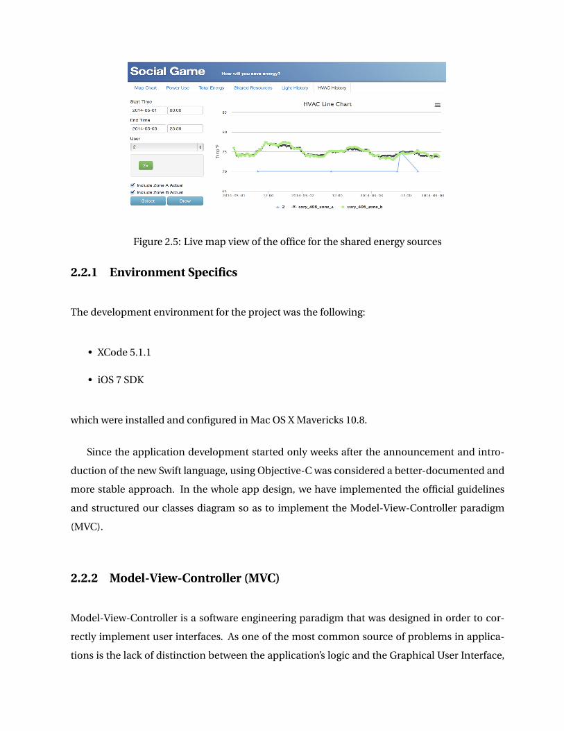
Figure 2.5: Live map view of the office for the shared energy sources

2.2.1 Environment Specifics

The development environment for the project was the following:

• XCode 5.1.1

• iOS 7 SDK

which were installed and configured in Mac OS X Mavericks 10.8.

Since the application development started only weeks after the announcement and intro-

duction of the new Swift language, using Objective-C was considered a better-documented and

more stable approach. In the whole app design, we have implemented the official guidelines

and structured our classes diagram so as to implement the Model-View-Controller paradigm

(MVC).

2.2.2 Model-View-Controller (MVC)

Model-View-Controller is a software engineering paradigm that was designed in order to cor-

rectly implement user interfaces. As one of the most common source of problems in applica-

tions is the lack of distinction between the application’s logic and the Graphical User Interface,

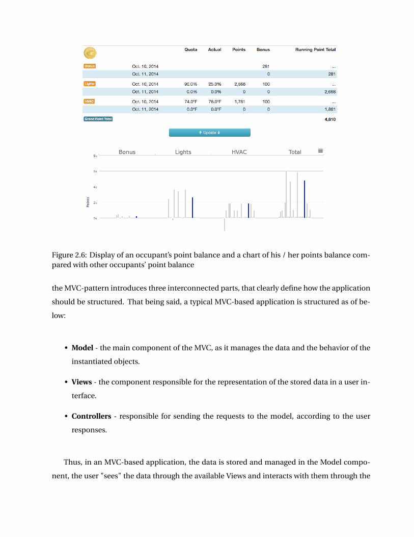
Figure 2.6: Display of an occupant’s point balance and a chart of his / her points balance com-pared with other occupants’ point balance

the MVC-pattern introduces three interconnected parts, that clearly define how the application

should be structured. That being said, a typical MVC-based application is structured as of be-

low:

• Model - the main component of the MVC, as it manages the data and the behavior of the

instantiated objects.

• Views - the component responsible for the representation of the stored data in a user in-

terface.

• Controllers - responsible for sending the requests to the model, according to the user

responses.

Thus, in an MVC-based application, the data is stored and managed in the Model compo-

nent, the user "sees" the data through the available Views and interacts with them through the

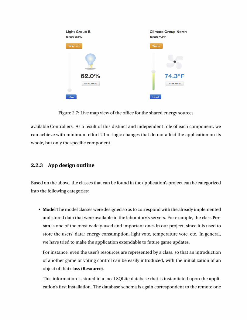
Figure 2.7: Live map view of the office for the shared energy sources

available Controllers. As a result of this distinct and independent role of each component, we

can achieve with minimum effort UI or logic changes that do not affect the application on its

whole, but only the specific component.

2.2.3 App design outline

Based on the above, the classes that can be found in the application’s project can be categorized

into the following categories:

• Model The model classes were designed so as to correspond with the already implemented

and stored data that were available in the laboratory’s servers. For example, the class Per-

son is one of the most widely-used and important ones in our project, since it is used to

store the users’ data: energy consumption, light vote, temperature vote, etc. In general,

we have tried to make the application extendable to future game updates.

For instance, even the user’s resources are represented by a class, so that an introduction

of another game or voting control can be easily introduced, with the initialization of an

object of that class (Resource).

This information is stored in a local SQLite database that is instantiated upon the appli-

cation’s first installation. The database schema is again correspondent to the remote one

and to the JSON responses that are available from the server.

The local database is synchronized and updated through asynchronous HTTP requests. It

should be noted, that the calls have been properly designed so as to ensure the security of

the server, but also possibly provide audit information as to which users use the app more

frequently. That being said, each user has a personal authentication token, which is stored

in the server. Upon log-in this token is retrieved, and all transaction and communication

calls that are made use this token, so as to authenticate with the server. This token is

destroyed when the user logs out, so as to prevent unauthorized calls.

• Views

The main user interface is defined in a .storyboard file. Through XCode’s development

environment, we can easily define the UI elements of each view, and their relationships.

In our app design, we have used one storyboard file for the iPhone devices and one for the

iPad ones.

• Controllers Every screen that the user sees is controlled by a View-Controller. In order to

write custom logic behind it, we have created for almost all views their respective View-

Controller class, which inherit from the UIViewController class that the iOS provides.

Therefore, the behavior of the UI elements that are defined in our views are handled by

this category of classes. For exampling, buttons’ events (e.g. tap) are handled through

these controllers, that in their turn make calls to the SQLite database or HTTP requests

that are available through the model’s classes.

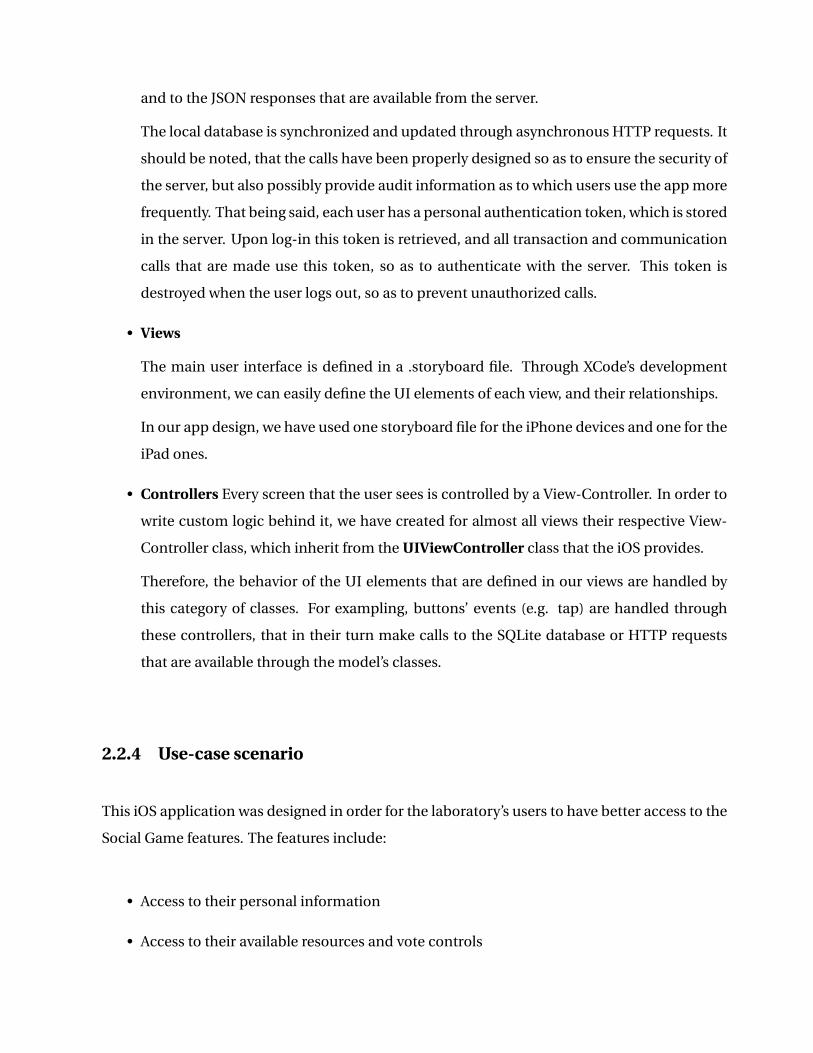
2.2.4 Use-case scenario

This iOS application was designed in order for the laboratory’s users to have better access to the

Social Game features. The features include:

• Access to their personal information

• Access to their available resources and vote controls

• Check-in/out mechanism for the game purposes

• Access to their weekly points, as well as statistics about the game previous winners

• A visual representation of the laboratory’s users, their votes and energy consumption.

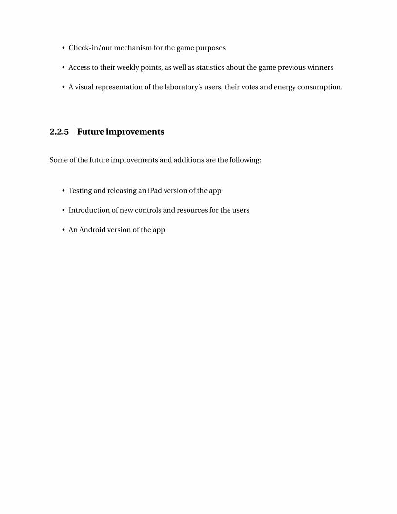
2.2.5 Future improvements

Some of the future improvements and additions are the following:

• Testing and releasing an iPad version of the app

• Introduction of new controls and resources for the users

• An Android version of the app

ViewControllersLoginViewController

TabSettingsViewController

TabControlViewController

TabChartsViewController

TabMapViewController

WinnersViewController

ChartsGraphsController

…

ViewsUIButton

UILabel

PointsCell

ResourceCell

WinnersCell

MessageCell

…

ModelStats

ChartItem

Message

Person

Office

Winner

Resource

DBManager

HTTPHandler

…

Figure 2.8: The MVC structure of the project’s classes

Figure 2.9: Left: The home tab - providing user info and announcements. Right: the user pointsand statistics

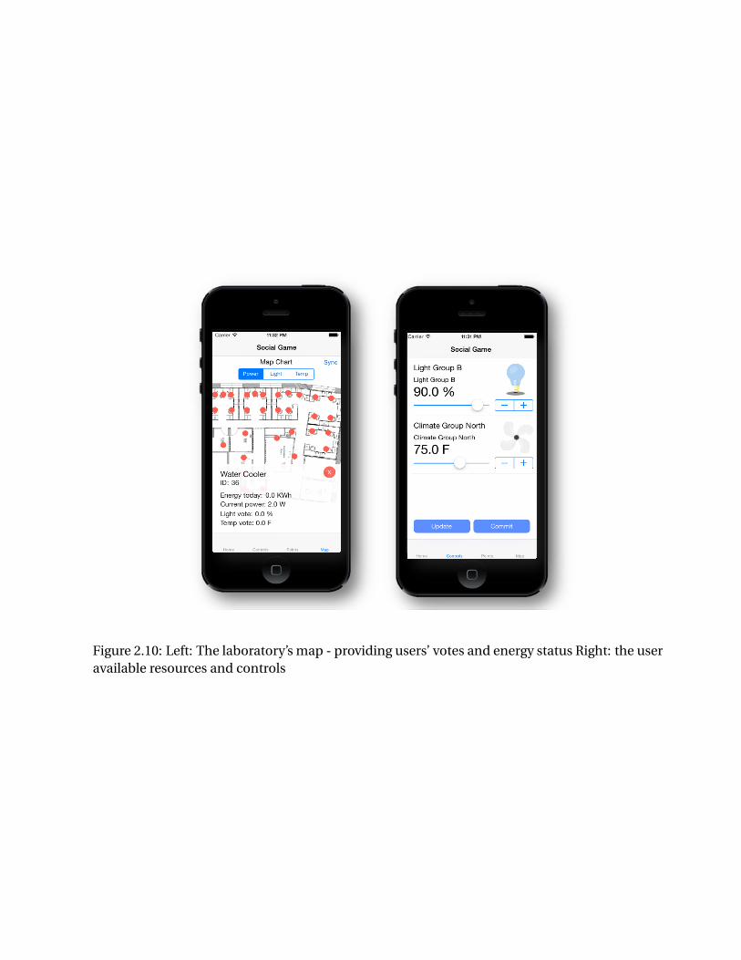
Figure 2.10: Left: The laboratory’s map - providing users’ votes and energy status Right: the useravailable resources and controls

Chapter 3

Game Formulation

We model the interaction between the building manager (leader) and the occupants (followers)

as a leader-follower type game. We use the terms leader and building manager interchageably

and similarly for follower and occupant.

In this model the followers are utility maximizers that play in a non-cooperative game for

which we use the Nash equilirbium concept. The leader is also a utility maximizer with a utility

that is dependent on the choices of the followers. The leader can influence the equilibrium of

the game amongst the followers through the use of incentives and default values of the light

as well as to the temperature level, which impact the utility and thereby the decisions of each

follower.

The leader desires to reduce the energy consumption in the building as well as formulate a

model of how the occupants make decisions about their energy usage. In order to achieve this

goal, the leader implements a social game in which the followers are pitted against one another.

The occupants win points based on their energy consumption choices. These points are then

used to determine the individual follower’s chance at winning in a lottery. The occupants select

the lighting and HVAC setting that they want to be implemented in the office. Actually, based

on the votes of the occupants we implement at the office as the lighting and HVAC setting the

average of all the occupants’ votes.

18

3.1 Follower Game

We will model the interaction between the occupants and their behavior by the usage of game

theory. Game theory for modeling the behavior of the occupants has several advantages. First,

it is a natural way to model agents competiting over resources. In our Social Game the resources

that the agents compete for them are the Amazon cards or possible other gift cards. Moreover,

it can also be leveraged in the design of incentives for behavioral change. It is essential for the

building manager to have an accurate model which incorporates the ability to model the occu-

pants as strategic players. In that way, a possible accurate agents’ model can capture a possible

change in their behavior resulting from a mixture of different incentives (and default values in

our game) of the building manager.

Let the number of occupants participating in the game be denoted by n. We model the oc-

cupants as utility maximizers having utility functions composed of two terms that capture the

trade off between comfort and desire to win. The usage of utility functions with two terms has

been done for simplicity in the utility estimation and since we assume that with the choice of

these two terms we can capture the trade off between comfort and desire to win. It is upon

research the investigation of more accurate class of functions that can be considered as appro-

priate terms for the agents’ utility functions.

We model their comfort level using a Taguchi loss function which is interpreted as model-

ing occupant dissatisfaction as increasing as variation increases from their desired lighting and

HVAC setting. In particular, each occupant has the following Taguchi loss function as one com-

ponent of their utility function:

ψi (xi , x−i ) =− (x −xi )2 (3.1)

where xi ∈ R is occupant i ’s lighting vote, x−i = x1, . . . , xi−1, xi+1, . . . , xn, and

x = 1

n

n∑i=1

xi (3.2)

is the average of all the occupant votes and is the lighting setting which is implemented. Each

occupant’s desire to win is modeled using the following function

φi (xi , x−i ) = ρ( xi

100

)2(3.3)

where ρ is the total number of points distributed by the building manager every day and xb is

the baseline setting for the lights and HVAC. The lighting baseline is considered 90 since the

lights were as an average in this setting before the beginning of the experiment. Also, the HVAC

baseline setting is 74 (Fahrenheit degrees) which has been selected as an appropriate temperate

comfort level. As the agents vote the points are dynamically distributed by the leader using the

relationship:

ρxb −xi

nxb −∑n

j=1 x j. (3.4)

Thus, a natural way to model occupant’s desire to win (function φi ) is by the usage of the

natural log function. This can clearly capture the way that the points are distributed to the occu-

pants in our experiment. Furthermore, it has the ability to represent the insensitivity threshold.

Figure 3.1 shows the relationship between the utility and the total wealth. It is clear that there is

a saturation point in which additional wealth respond to a small range of behavioral change.

We found that the form of φi as defined in (3.3) provides a better estimation and prediction

of the occupant’s behavior. It appears that it captures the occupants’ perceptions about how the

points are distributed and their value more accurately. Also, it seems that the incentives that we

currently apply in our experiment aren’t so close to the insensitivity threshold and the function

that model the desire to win works properly.

Each occupant’s utility function is given by:

fi (xi , x−i ) =ψi (xi , x−i )+θiφi (xi , x−i ) (3.5)

where θi is an unknown parameter.

Problem'for''Real'Money'Back'Game'

•  People'just'don’t'care…'

Total'Wealth'0'

U4lity'

Insensi4vity'

Threshold'

Current''Money'

Very'small'range'for''behavior'change'

System'gives''Real'Money''back'to'user'

Figure 3.1: Human utility behavior

The occupants face the following optimization problem:

maxxi∈Si

fi (xi , x−i ) (3.6)

where Si = [0,100] ⊂ R is the constraint set for each xi .

Note that each occupant’s optimization problem is dependent on the other occupant’s choice

variables. We can explicitly write out the constraint set as follows. Let hi , j (xi , x−i ) for j ∈ 1,2

denote the constraints on occupant i ’s optimization problem. In particular, following Rosen [25],

for occupant i , the constraints are (for the light setting):

hi ,1(xi ) = 100−xi (3.7)

hi ,2(xi ) = xi (3.8)

Without loss of generality the constraints for HVAC are:

hi ,1(xi ) = 78−xi (3.9)

hi ,2(xi ) = xi −70 (3.10)

Our analysis will be based on the lighting constraints. However, the results can be general-

ized for the HVAC too. So, we can define Ci = xi ∈ R| hi , j (xi ) ≥ 0, j ∈ 1,2 and C =C1×·· ·×Cn .

Thus, the occupants are non-cooperative agents in a continuous game with convex constraints.

We model their interaction using the Nash equilibrium concept.

Definition 1. A point x ∈C is a Nash equilibrium for the game ( f1, . . . , fn) on C if

fi (xi , x−i ) ≥ fi (x ′i , x−i ) ∀ x ′

i ∈Ci (3.11)

for each i ∈ 1, . . . ,n.

The definition of Nash equilibrium is a point from which no player can increase his/her utility

by a unilateral change in their strategy. If the parameters θi ≥ 0, then the game is a concave n-

person game on a convex set.

Theorem 1 (Rosen [25]). A Nash equilibrium exists for every concave n-person game.

Define the Lagrangian of each player’s optimization problem as follows:

Li (xi , x−i ,µi ) = fi (xi , x−i )+ ∑j∈Ai (xi )

µi , j hi , j (xi ) (3.12)

where Ai (xi ) is the active constraint set at xi .

We can define

ω(x,µ) =

D1L1(x,µ1)

...

DnLn(x,µn)

(3.13)

where Di Li denoets the derivative of Li with respect to xi .

It is the local representation of the differential game form [21] corresponding to the game

between the occupants.

Definition 2 (Ratliff, et al. [21]). A point x∗ ∈ C is a differential Nash equilibrium for the game

( f1, . . . , fn) on C ifω(x∗,µ∗) = 0, zT Di i Li (x∗,µ∗i )z < 0 for all z 6= 0 such that Di hi , j (x∗

i )T z = 0, and

µi , j > 0 for j ∈ Ai (x∗i ).

Proposition 1. A differential Nash equilibrium of the n-person concave game ( f1, . . . , fn) on C is

a Nash equilibrium.

Proof. The proof is straightforward. Indeed, suppose the assumptions hold. The constraints for

each player do not depend on other players’ choice variables. We can hold x∗−i fixed and apply

Proposition 3.3.2 [3] to the i -th player’s optimization problem

maxxi∈Ci

fi (xi , x∗−i ) (3.14)

Since each fi is concave and each Ci is a convex set, x∗i is a global optimum of the i -th

player’s optimization problem under the assumptions. Since this is true for each of the i ∈1, . . . ,n players, x∗ is a Nash equilibrium.

A sufficient condition guaranteeing that a Nash equilibrium x is isolated is that the Jaco-

bian of ω(x,µ), denoted Dω(x,µ), is invertible [21],[25]. We refer to such points as being non-

degenerate.

3.2 Leader Optimization Problem – Incentive Design

A reverse Stackelberg game is a hierarchical control problem in which sequential decision mak-

ing occurs; in particular, there is a leader that announces a mapping of the follower’s decision

space into the leader’s decision space, after which the follower determines his optimal deci-

sion [9].

Both the leader and the followers wish to maximize their pay-off determined by the functions

fL(x, y) and f1(x,γ(x)), . . . , fn(x,γ(x)) respectively where we now consider each of the follower’s

utility functions to be a function of the incentive mechanism γ : x 7→ y where leader’s decision

is y = (d ,ρ) with d being the default lighting setting and ρ the total number of points. The

followers’ decisions is denoted by x. The leader’s strategy is γ.

The basic approach to solving the reversed Stackelberg game is as follows. Let y and x take

values in Y ⊂ R2 and Ci ⊂ R, respectively and let fL , fi : Rn ×R2R for each i ∈ 1, . . . ,n. We define

the desired choice for the leader as

(x∗, y∗) ∈ argmaxx,y

fL(x, y)| y ∈ Y , x ∈C . (3.15)

Of course, if fL is concave and Y ×C is convex, then the desired solution is unique. The incen-

tive problem can be stated as follows: Find γ : X Y , γ ∈ Γ such that x∗ is a differential Nash

equilibrium of the follower game ( f1, . . . , fn) subject to constraints and γ(x∗) = y∗ where Γ is the

set of admissible incentive mechanisms. By insuring that the desired agent action x∗ is a non-

degenerate differential Nash equilibrium ensures structural stability of equilibrium helping to

make the solution robust to measurement and environmental noise [22]. Further, it insures that

it is (locally) isolated — it is globally isolated if the followers’ game is concave.

For the lighting social game, the leader’s utility function is given as follows:

fL(x, y) =E[

K − g (y, x)︸ ︷︷ ︸ener g y

−c2p(ρ)︸ ︷︷ ︸e f f or t

− c1

n∑i=1

βi fi (xi , x−i , y)︸ ︷︷ ︸benevolence

](3.16)

where K is is the maximum consumption of the Lutron lighting system in kilowatt-hours (kWh),

g (y, x) is the is the energy consumption in kWh at a given (y, x), p(·) is a cost-for-effort function

on the points ρ and c1,c2 ∈ R+ are scaling factors for the last two terms describing how much

utility and total points respectively the leader is willing to exchange for 1 kWh. The last term is

the benevolence term where the βi ’s are the benevolence factors. This term captures the fact that

the leader to cares about the followers’ satisfaction which is related to their productivity level

(see [23] for a similar formulation). The expectation is taken with respect to the joint distribution

defined by distributions across the player states absent, active, default.

Due to the complexity of computing this expectation, we currently restrict the set of admis-

sible incentive mechanisms to be the constant map γ(x) = (d ,ρ) for all x so that the leader only

selects the constants (d ,ρ). This reduces the solution of the reversed Stackelberg game to a bi-

level optimization problem. We are exploring more general classes of incentive mechanisms.

Since the prize in the lottery is currently a fixed monetary value delivered to the winner

through an Amazon gift card, varying the points does not cost the leader anything explicitly.

However, we model the cost of giving points by a function p(·) which captures the fact that after

some critical value of ρ the points no longer seem as valuable to the followers, in the sense that

it becomes difficult for them to perceive the true value of the points as they affect the follower’s

chances of winning. It is clear that the occupants follow the log function and the incentives

doesn’t affect them. It is upon research the effect of different kind of prizes.

The followers’ perceive the points that they receive has having some value towards winning

the prize. The leader’s goal is to choose ρ and d so they induce the followers to play the game

and choose the desired lighting setting but not to increase the points beyond a level after which

it becomes difficult for the followers to perceive the true value of the points.

Currently we do not add individual rationality constraints to the leader’s optimization prob-

lem which would ensure that the players’ utilities are at least as much as what they would get

by selecting the default value. The impact being that this constraint would ensure players are

active. With respect to economics literature, the default lighting setting compares to the outside

option in contract theory. It is interesting that in the current situation the leader has control

over the outside option. We leave exploring this for future work.

Due to the complexity of computing the expectation for the joint distribution across player

states absent, active, default for n = 20 players, we currently restrict the set of admissible incen-

tive mechanisms to be the map γ(x) = (γd (x),γρ(x)) such that the i -th player’s utility is

fi (x,γ(x)) =ψi (x)−θiγρ(x)( xi

100

)2(3.17)

where γ(x) ≡ ρ for all i ∈ 1, . . . ,n. In addition, the nature of γd (x) is that it is an option provided

to the followers; they must actively vote in order for this value not to be taken as their current

vote when they are present in the office. In sense, it is the outside option. Thus, the leader only

selects the constants (d ,ρ). This reduces the solution of the reversed Stackelberg game to a bi-

level optimization problem that we solve with a particle swarm optimization (PSO) technique

(see, e.g., [10, 11, 27]).

The particle swarm optimization method is a population based stochastic optimization tech-

nique in which the algorithm is initialized with a population of random solutions and searches

for optima by updating generations. The potential solutions are called particles. Each parti-

cle stores its coordinates in the problems space which are associated with the best solution

achieved up to the current time. The best over all particles is also stored and at each iteration

the algorithm updates the particles’ velocities.

At the inner level of the bi-level optimization problem, we replace the condition that the

occupants play a Nash equilibrium with the dynamical system determined by the gradients of

each player’s utility with respect to their own choice variable, i.e.

xi = Di fi (xi , x−i , y), xi ∈Ci , ∀ i ∈ 1, . . . ,n. (3.18)

It has been shown that by using a projected gradient descent method for computing sta-

tionary points of the dynamical system in (3.18), which is derived from an n-person concave

games on convex strategy spaces, converges to Nash equilibria [8]. In our simulations, we add

the constraint to the leader’s optimization problem that at the stationary points of this dynam-

ical system, i.e. the Nash equilibria, the matrix −Dω is positive definite thereby ensuring that

each of the equilibria are non-degenerate and hence, isolated.

Denote the set of non-degenerate stationary points of the dynamical system x as defined

in (3.18) as Stat(x). The leader then solves the following problem: given the joint distribution

across player states active, default, absent, find

maxy∈Y

fL(y, x) (3.19)

s.t. x ∈ Stat(x)

For each particle in the PSO algorithm, we sample from the distribution across player states

and compute Nash equilibrium points for the resulting game via simulation of the dynamical

system (3.18). We compute the mean of the votes at the Nash equilibrium to get the lighting

setting. We repeat this process and use the mean of the lighting settings over all the simula-

tions to compute the leader’s utility for each of the particles. We are currently exploring other

techniques for solving bi-level optimization problems in which the degree of complexity of com-

puting leader’s utility is very high.

The leader changes ρ to a value that the followers perceive as translating into more value

towards winning in the lottery. We remark that the points ρ do not show up in the leader’s utility

explicitly due to the fact that the prizes in the lottery are currently fixed and the leader can vary

the points but it does not actually cost anything to vary these points. The goal in choosing the

value of ρ is to see how the players perceive the value of points even though the prize in the

lottery is fixed.

Chapter 4

Utility Estimation

We formulate the utility estimation problem as a convex optimization problem by using first-

order necessary conditions for Nash equilibria. In particular, the gradient of each occupant’s

utility function should be identically zero at the observed Nash equilibrium. This is the case

since the observed Nash equilibria are all inside the feasible region so that none of the con-

straints are active, i.e. we do not have to check the derivative of Lagrangian of each occupant’s

optimization problem.

For each observation x(k), we assume that it corresponds to occupants playing a strategy

that is approximately a Nash equilibrium where the superscript notation (·)(k) indicates the k-th

observation. Thus, we can consider first-order optimality conditions for each occupants op-

timization problem and define a residual function capturing the amount of sub-optimality of

each occupants choice x(k)i [12],[23].

Again, since all our observations are on the interior of the constraint set, we consider the

residual defined by the stationarity and complementary slackness conditions for each occu-

pant’s optimization problem:

28

r (k)s,i (θi ,µi ) = Di fi (x(k)

i , x(k)−i )+

n∑j=1

µji Di hi , j (x(k)

i ) (4.1)

r j ,(k)c,i (µ) =µ j

i hi , j (x(k)i ) j ∈ 1,2 (4.2)

Define r (k)s (θ) = [r (k)

s,1 (θ1,µ1) · · · r (k)s,n (θn ,µn)]T and r (k)

c,i (µi ) = [r 1,(k)c,i (µi ) r 2,(k)

c,i (µi )] so that we

can define r (k)c = [r (k)

c,1 (µ1) · · · r (k)c,n(µn)]T where µi = (µ1

i ,µ2i ).

Given observations x(k)Kk=1 where each x(k) ∈ C , we can solve the following convex opti-

mization problem:

minµ,θ

K∑k=1

χ(r (k)s (θ,µ),r (k)

c (µ)) (4.3)

s.t. θi ≥ 0,µi ≥ 0 ∀ i ∈ 1, . . . ,n (4.4)

where χ : Rn ×R2nR+ is a nonnegative, convex penalty function satisfying χ(z1, z2) = 0 if and

only if z1 = 0 and z2 = 0, i.e. any norm on Rn ×R2n , and the inequality µi ≥ 0 is elementwise.

Note that we constrain the θi ’s to be non-negative. This is to ensure that the estimated utility

functions are concave. We add this restriction so that we can employ techniques from simula-

tion of dynamical systems to the computation of the Nash equilibrium in the resulting n-person

concave game with convex constraints. In particular, define a gradient-like system using the lo-

cal representation of the differential game form [21] and using the estimated θi ’s

xi = Di fi (xi , x−i ;θi ) ∀ i ∈ 1, . . . ,n, (4.5)

and consider the feasible set defined by the constraints

hi ,1(xi ) = 100−xi ≥ 0

hi ,2(xi ) = xi ≥ 0

∀ i ∈ 1, . . . ,20 (4.6)

Then, as we mentioned in the previous section, the subgradient projection method applied

to the dynamics (4.5) and the constraint set defined by (4.6) is known to converge to the unique

Nash equilibrium of the constrained n-person concave game [8].

For the proposed estimation we apply the bootstrapping method to obtain the empirical

distribution of θi for i ∈ 1, ...,20 by randomly sampling a subset from the data [7]. Thus, we

have as result different histograms for each user for the estimated parameter θi .

We use these histograms as to have more accurate estimations of the unknown parameters

θi as well as to reduce the residual error. Moreover, we use the histograms and the resulting

empirical distributions in order to obtain the mean value of the θi parameters. Last but not

least, based on the mean values of the θi parameters we calculate the resulting Nash equilibrium

points and we predict the occupants’ next day lighting and HVAC vote.

Chapter 5

Results

In this chapter we report the results on the savings achieved through the game, the utility learn-

ing problem as well as simulation of the estimated utilities. Moreover, by the collected data on

the energy consumption of the lights for different lighting settings we have created an utility

function for the leader so as to solve the incentive design problem. We present by simulations

that with an optimal selection of the default values for the lights as well as for the points we can

achieve an energy efficient light level.

5.1 Utility estimations - Energy savings

We use the data collected over the period from March 3, 2014 to June 16, 2014 when occupants

have regular working schedules in the office. The baseline xb is 90% for lighting, and 74 Fahren-

heit degrees for the HVAC, which was the standard lighting and HVAC level prior to the begin-

ning of the experiment. Throughout this period, we have changed the default lighting level three

times (see Table 5.1).

We divide each day into four regions based on the outside lighting in Berkeley during the

summer, namely from 7am to 12pm (Morning), 12pm to 5pm (Early afternoon), 5pm to 10pm

(Late afternoon), and 10pm to the next day 7am (Night). The data is further processed by taking

31

Period Default Level

March 3–April 10 20 %April 11–May 1 10 %May 2–May 23 60 %

May 24 – June 16 90 %

Table 5.1: Default levels for four periods during the experiment. By changing the default settingto 90% we isolate the savings due to the social game from those achieved by changing the defaultsetting.

the average of votes in each region of the day for each user.

5.1.1 Savings

Using the mean savings for each of the periods and a rate of $0.12/kWh we estimate that we

saved $73. In addition, over the period of 101 days that the experiment was conducted the of-

fice consumed 2,185 kWh for lighting and we saved approximately 601 kWh. That is a 27.5%

reduction in energy. This savings is just due to a change in lighting usage behavior for one small

portion of a building.

Figure 5.1: Lights’ average daily dim level

As we can see in Figure 5.1 we had a significant reduction in the actual lights’ power setting

through the experiment. Furthermore, in Figure 5.2 we can see a crucial reduction in total daily

energy consumption in the office. However, it is upon investigation how much the default level

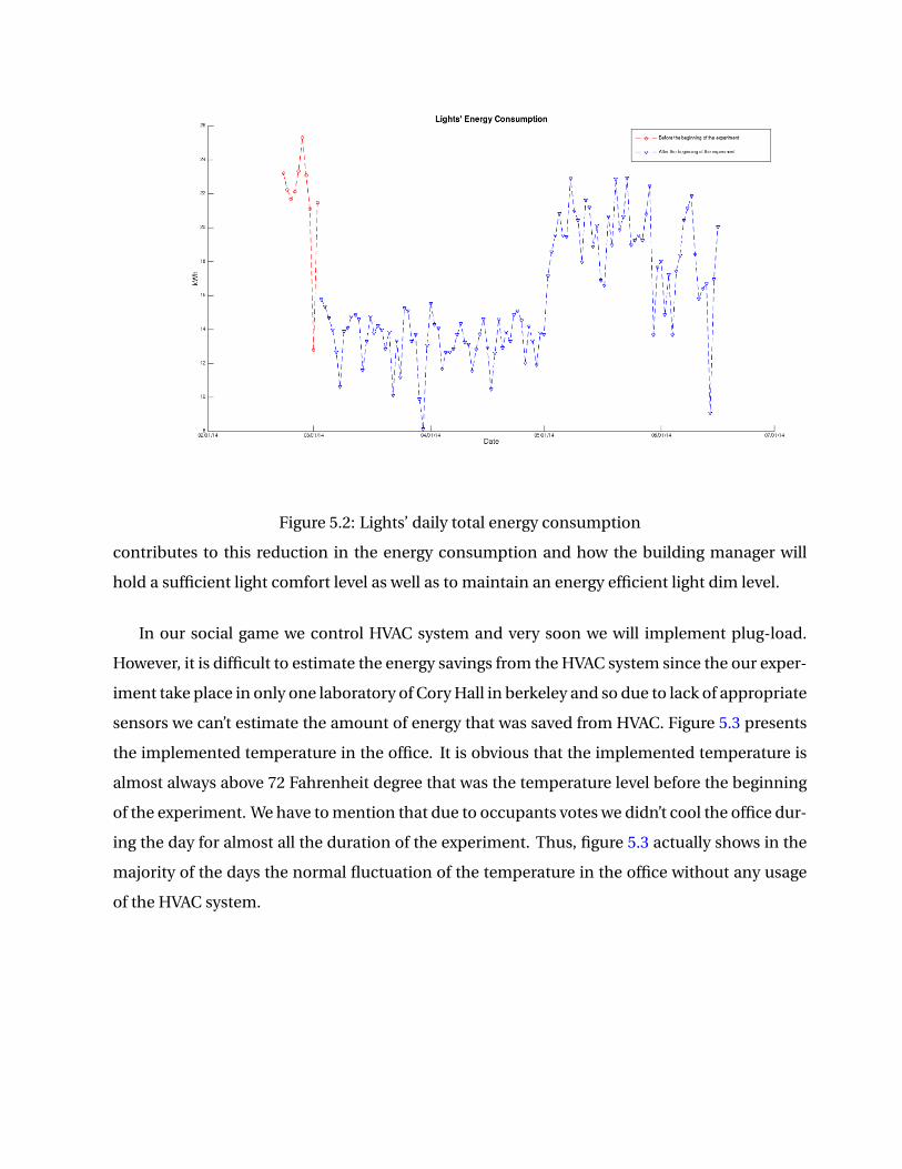
Figure 5.2: Lights’ daily total energy consumption

contributes to this reduction in the energy consumption and how the building manager will

hold a sufficient light comfort level as well as to maintain an energy efficient light dim level.

In our social game we control HVAC system and very soon we will implement plug-load.

However, it is difficult to estimate the energy savings from the HVAC system since the our exper-

iment take place in only one laboratory of Cory Hall in berkeley and so due to lack of appropriate

sensors we can’t estimate the amount of energy that was saved from HVAC. Figure 5.3 presents

the implemented temperature in the office. It is obvious that the implemented temperature is

almost always above 72 Fahrenheit degree that was the temperature level before the beginning

of the experiment. We have to mention that due to occupants votes we didn’t cool the office dur-

ing the day for almost all the duration of the experiment. Thus, figure 5.3 actually shows in the

majority of the days the normal fluctuation of the temperature in the office without any usage

of the HVAC system.

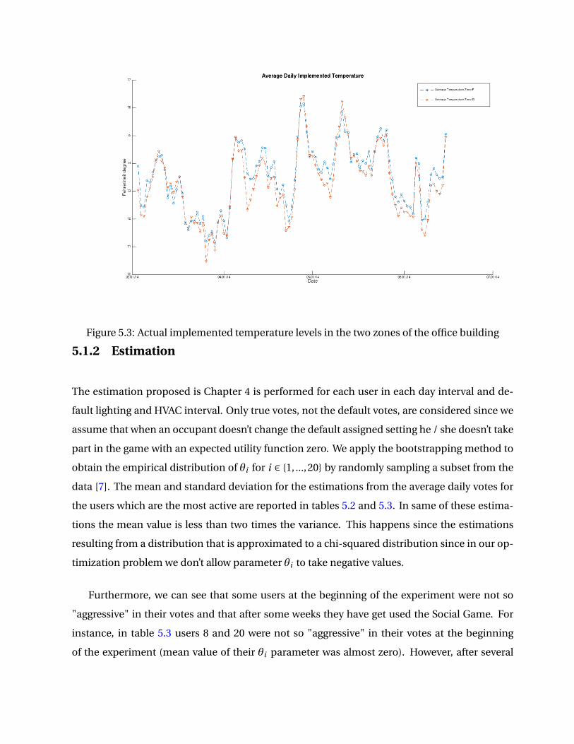
Figure 5.3: Actual implemented temperature levels in the two zones of the office building

5.1.2 Estimation

The estimation proposed is Chapter 4 is performed for each user in each day interval and de-

fault lighting and HVAC interval. Only true votes, not the default votes, are considered since we

assume that when an occupant doesn’t change the default assigned setting he / she doesn’t take

part in the game with an expected utility function zero. We apply the bootstrapping method to

obtain the empirical distribution of θi for i ∈ 1, ...,20 by randomly sampling a subset from the

data [7]. The mean and standard deviation for the estimations from the average daily votes for

the users which are the most active are reported in tables 5.2 and 5.3. In same of these estima-

tions the mean value is less than two times the variance. This happens since the estimations

resulting from a distribution that is approximated to a chi-squared distribution since in our op-

timization problem we don’t allow parameter θi to take negative values.

Furthermore, we can see that some users at the beginning of the experiment were not so

"aggressive" in their votes and that after some weeks they have get used the Social Game. For

instance, in table 5.3 users 8 and 20 were not so "aggressive" in their votes at the beginning

of the experiment (mean value of their θi parameter was almost zero). However, after several

weeks they voted with an energy efficient way in order they to gain more points and increase

their likelihood of winning the lottery. Furthermore, for the four regions based on the outside

lighting in Berkeley during the summer the estimation method is exactly the same and we can

derive important information about the light and HVAC level during specific time intervals in a

day. Finally, in figure 5.4 and figure 5.5 we can see the histograms of the θi of two participants

for their average daily votes in the default region 20.

Figure 5.4: User 8 light histogram of estimation of θi in the default region 20

Figure 5.5: User 14 light histogram of estimation of θi in the default region 20

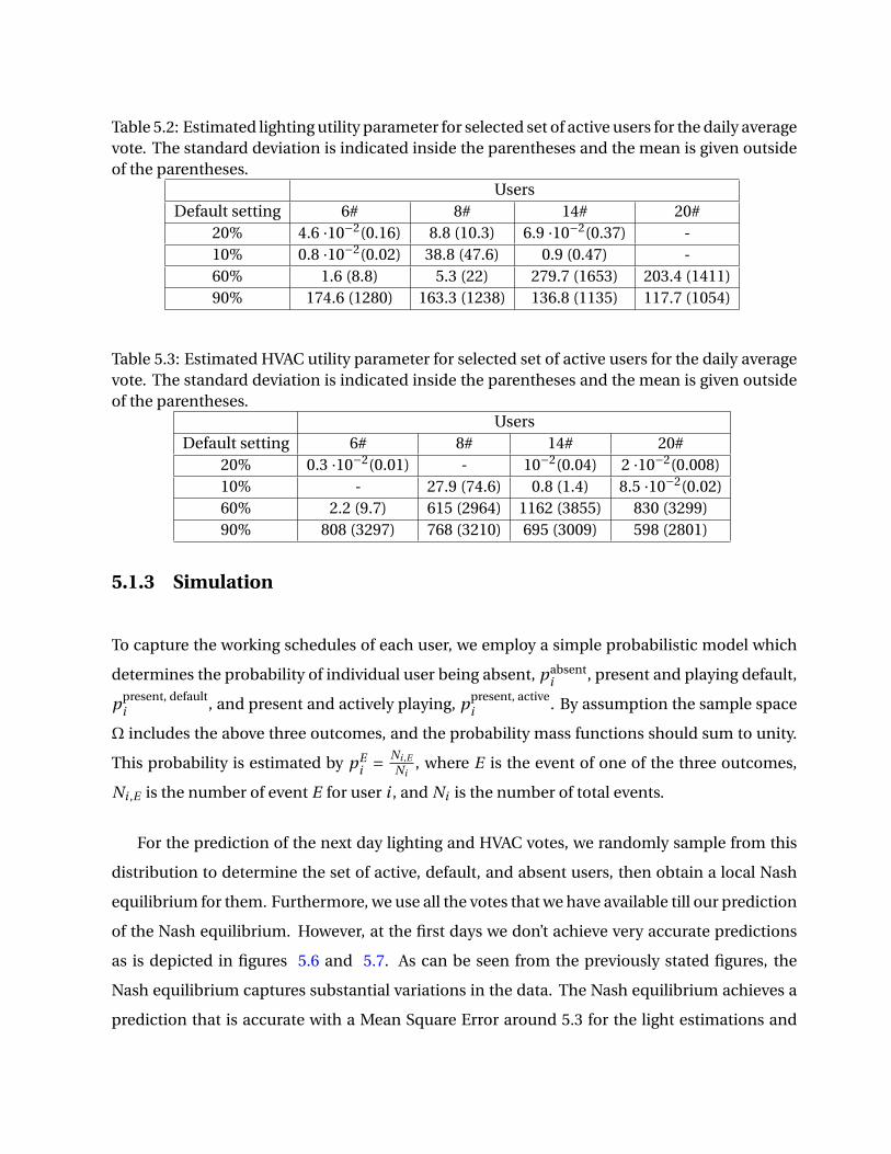
Table 5.2: Estimated lighting utility parameter for selected set of active users for the daily averagevote. The standard deviation is indicated inside the parentheses and the mean is given outsideof the parentheses.

UsersDefault setting 6# 8# 14# 20#

20% 4.6 ·10−2(0.16) 8.8 (10.3) 6.9 ·10−2(0.37) -10% 0.8 ·10−2(0.02) 38.8 (47.6) 0.9 (0.47) -60% 1.6 (8.8) 5.3 (22) 279.7 (1653) 203.4 (1411)90% 174.6 (1280) 163.3 (1238) 136.8 (1135) 117.7 (1054)

Table 5.3: Estimated HVAC utility parameter for selected set of active users for the daily averagevote. The standard deviation is indicated inside the parentheses and the mean is given outsideof the parentheses.

UsersDefault setting 6# 8# 14# 20#

20% 0.3 ·10−2(0.01) - 10−2(0.04) 2 ·10−2(0.008)10% - 27.9 (74.6) 0.8 (1.4) 8.5 ·10−2(0.02)60% 2.2 (9.7) 615 (2964) 1162 (3855) 830 (3299)90% 808 (3297) 768 (3210) 695 (3009) 598 (2801)

5.1.3 Simulation

To capture the working schedules of each user, we employ a simple probabilistic model which

determines the probability of individual user being absent, pabsenti , present and playing default,

ppresent, defaulti , and present and actively playing, ppresent, active

i . By assumption the sample space

Ω includes the above three outcomes, and the probability mass functions should sum to unity.

This probability is estimated by pEi = Ni ,E

Ni, where E is the event of one of the three outcomes,

Ni ,E is the number of event E for user i , and Ni is the number of total events.

For the prediction of the next day lighting and HVAC votes, we randomly sample from this

distribution to determine the set of active, default, and absent users, then obtain a local Nash

equilibrium for them. Furthermore, we use all the votes that we have available till our prediction

of the Nash equilibrium. However, at the first days we don’t achieve very accurate predictions

as is depicted in figures 5.6 and 5.7. As can be seen from the previously stated figures, the

Nash equilibrium captures substantial variations in the data. The Nash equilibrium achieves a

prediction that is accurate with a Mean Square Error around 5.3 for the light estimations and

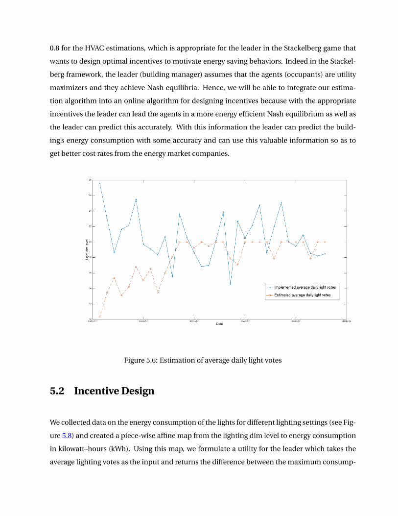
0.8 for the HVAC estimations, which is appropriate for the leader in the Stackelberg game that

wants to design optimal incentives to motivate energy saving behaviors. Indeed in the Stackel-

berg framework, the leader (building manager) assumes that the agents (occupants) are utility

maximizers and they achieve Nash equilibria. Hence, we will be able to integrate our estima-

tion algorithm into an online algorithm for designing incentives because with the appropriate

incentives the leader can lead the agents in a more energy efficient Nash equilibrium as well as

the leader can predict this accurately. With this information the leader can predict the build-

ing’s energy consumption with some accuracy and can use this valuable information so as to

get better cost rates from the energy market companies.

Figure 5.6: Estimation of average daily light votes

5.2 Incentive Design

We collected data on the energy consumption of the lights for different lighting settings (see Fig-

ure 5.8) and created a piece-wise affine map from the lighting dim level to energy consumption

in kilowatt–hours (kWh). Using this map, we formulate a utility for the leader which takes the

average lighting votes as the input and returns the difference between the maximum consump-

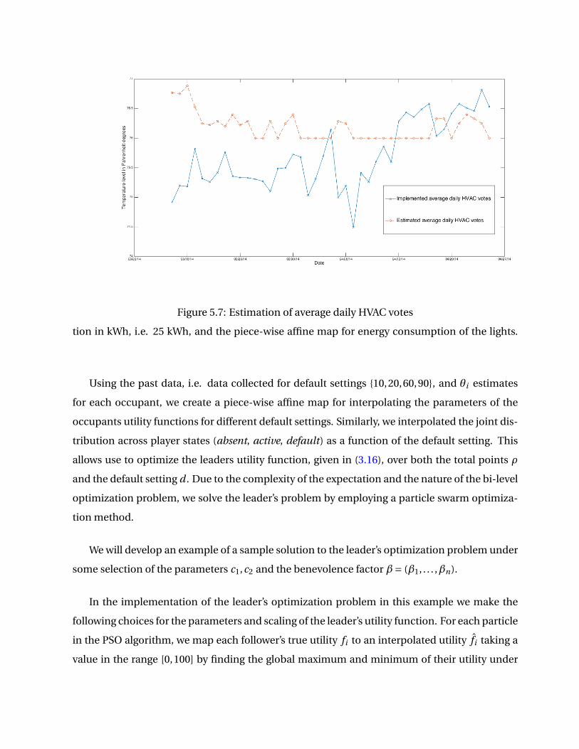
Figure 5.7: Estimation of average daily HVAC votes

tion in kWh, i.e. 25 kWh, and the piece-wise affine map for energy consumption of the lights.

Using the past data, i.e. data collected for default settings 10,20,60,90, and θi estimates

for each occupant, we create a piece-wise affine map for interpolating the parameters of the

occupants utility functions for different default settings. Similarly, we interpolated the joint dis-

tribution across player states (absent, active, default) as a function of the default setting. This

allows use to optimize the leaders utility function, given in (3.16), over both the total points ρ

and the default setting d . Due to the complexity of the expectation and the nature of the bi-level

optimization problem, we solve the leader’s problem by employing a particle swarm optimiza-

tion method.

We will develop an example of a sample solution to the leader’s optimization problem under

some selection of the parameters c1,c2 and the benevolence factor β= (β1, . . . ,βn).

In the implementation of the leader’s optimization problem in this example we make the

following choices for the parameters and scaling of the leader’s utility function. For each particle

in the PSO algorithm, we map each follower’s true utility fi to an interpolated utility fi taking a

value in the range [0,100] by finding the global maximum and minimum of their utility under

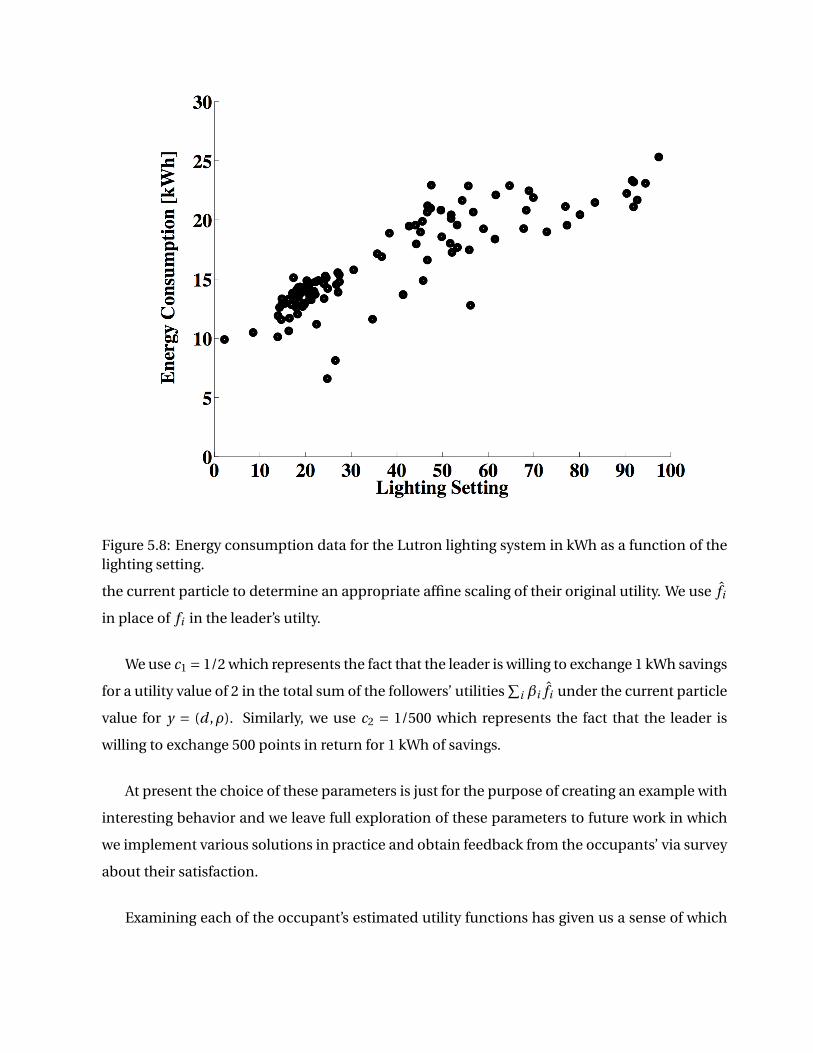
Figure 5.8: Energy consumption data for the Lutron lighting system in kWh as a function of thelighting setting.

the current particle to determine an appropriate affine scaling of their original utility. We use fi

in place of fi in the leader’s utilty.

We use c1 = 1/2 which represents the fact that the leader is willing to exchange 1 kWh savings

for a utility value of 2 in the total sum of the followers’ utilities∑

i βi fi under the current particle

value for y = (d ,ρ). Similarly, we use c2 = 1/500 which represents the fact that the leader is

willing to exchange 500 points in return for 1 kWh of savings.

At present the choice of these parameters is just for the purpose of creating an example with

interesting behavior and we leave full exploration of these parameters to future work in which

we implement various solutions in practice and obtain feedback from the occupants’ via survey

about their satisfaction.

Examining each of the occupant’s estimated utility functions has given us a sense of which

50

100

24 x 10

5

0

20

40

60

80

Incentive value, ρ

Default lighting, d

Figure 5.9: Utility of occupant 2 as a function of (d ,ρ) at the mean Nash equilibrium after run-ning 1000 simulations. Notice that for fixed values of d the utility value is near constant in ρ.Also, occupant 2 has very large utility when the default setting is around 70.

occupants are the most sensitive to changes in ρ and d . Occupant 2 is quite inflexible to changes

in the points ρ and appears to care less about winning and more about his comfort level (see

Figure 5.9). This fact is also reflected in the very low parameter estimate for θ2. It is also the case

that occupant 2’s behavior is largely affected by others’ votes.

In addition, occupants in the set C = 2,6,8,14,20 are the most active players in a proba-

bilistic sense. As a result, in this example we give non-zero benevolence terms to players in this

set. We refer to this set as the leader’s care-set. For all i ∈ 1, . . . ,20\C , we set βi = 0. Further,

we force∑

j∈C β j = 1. Since occupant 2 has particularly interesting behavior, we vary β2, and let

β j = (1−β2) 1|C | for all j ∈C and where |C | is the cardinality of C . 0.2cm

(d ,ρ,β2,∑

j∈Aβ j ) utility

(63,200×103,0.9,0.1) $4.56(56,169.6×103,0.75,0.25) $4.73(55.5,175.2×103,0.6,0.4) $4.67(48,142.2×103,0.45,0.55) $4.69(10.47,173×103,0.3,0.7) $5.07(7.23,194.6×103,0.2,0.8) $5.43

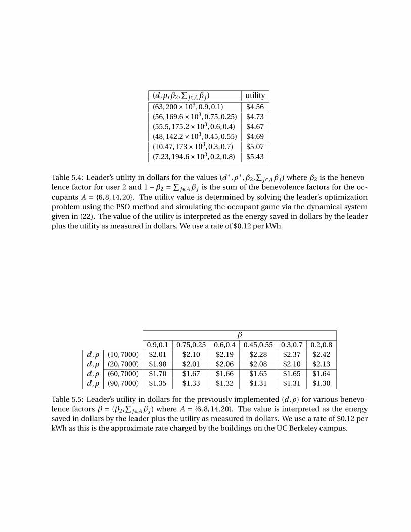
Table 5.4: Leader’s utility in dollars for the values (d∗,ρ∗,β2,∑

j∈Aβ j ) where β2 is the benevo-lence factor for user 2 and 1−β2 = ∑

j∈Aβ j is the sum of the benevolence factors for the oc-cupants A = 6,8,14,20. The utility value is determined by solving the leader’s optimizationproblem using the PSO method and simulating the occupant game via the dynamical systemgiven in (22). The value of the utility is interpreted as the energy saved in dollars by the leaderplus the utility as measured in dollars. We use a rate of $0.12 per kWh.

β

0.9,0.1 0.75,0.25 0.6,0.4 0.45,0.55 0.3,0.7 0.2,0.8d ,ρ (10,7000) $2.01 $2.10 $2.19 $2.28 $2.37 $2.42d ,ρ (20,7000) $1.98 $2.01 $2.06 $2.08 $2.10 $2.13d ,ρ (60,7000) $1.70 $1.67 $1.66 $1.65 $1.65 $1.64d ,ρ (90,7000) $1.35 $1.33 $1.32 $1.31 $1.31 $1.30

Table 5.5: Leader’s utility in dollars for the previously implemented (d ,ρ) for various benevo-lence factors β = (β2,

∑j∈Aβ j ) where A = 6,8,14,20. The value is interpreted as the energy

saved in dollars by the leader plus the utility as measured in dollars. We use a rate of $0.12 perkWh as this is the approximate rate charged by the buildings on the UC Berkeley campus.

Tables 5.5 and 5.4 contain the energy savings in dollars per day for the leader given the energy

cost of the lights and how much of the occupants’ utility and the total points distributed per

day that the leader is willing to exchange for 1 kWh in dollars using a cost per kWh of $0.12.

The values were computed by solving the leader’s optimization problem via the PSO method

where we simulate the game of the occupants via the dynamics system in (22). Table 5.5 has

the leader’s utility in dollars for previous values of (d ,ρ) after the start of the social game. In

Table 5.4 we report the values after optimizing over (d ,ρ) for some given benevolence factor

β = (β1, . . . ,βn). We can see that computing even the suboptimal (d ,ρ) by solving the leader’s

bi-level optimization problem via PSO, the leader has a much higher utility.

We have not yet factored in the cost of the prize in the lottery. Currently it is at a value

of $100 per week. The values we report in Tables 5.5 and 5.4 are per day savings on weekdays.

Hence, with a prize cost of $20 per day for our particular experimental set-up the leader does not

save. Using this case-study as proof-of-concept, we are in the process of implementing a social

game in an entire building in Singapore with more than 1,000 occupants. This social game will

include options for the consumer to choose lighting setting, HVAC and personal cubicle plug-

load consumption. In addition, we plan to implement a social game of this nature in Sutarja Dai

Hall on the UC Berkeley campus. At this scale, with a week-day lottery cost of $100 the building

manager stands to save a considerable amount.

In Figure 5.10, we show the results of simulating the game under the (d ,ρ)’s that we found

for various benevolence factors. We show the mean of the lighting votes averaged over 1000

simulations. It is interesting to see that the average Nash equilibrium under the various default

settings is actually less than the default setting itself except in the case when the default setting

is below a threshold below which occupants actually log votes above the default setting. For

example, with a default setting of 10.74, the mean of the Nash equilibria is ∼ 15. The case when

the default setting is above this threshold of basic operation, the most aggressive players’ desire

to win pushes the Nash equilibrium below the default. On the other hand, when the default is

below this threshold, all the players’ comfort comes into play and shifts the Nash equilibrium

above the default setting. This is likely due to the desire to win by the most aggressive players.

By examining user 2’s utility as a function of (d ,ρ), we determined that this occupant is the

most dissatisfied when the default lighting setting is below a setting of 70. Hence, we simulated

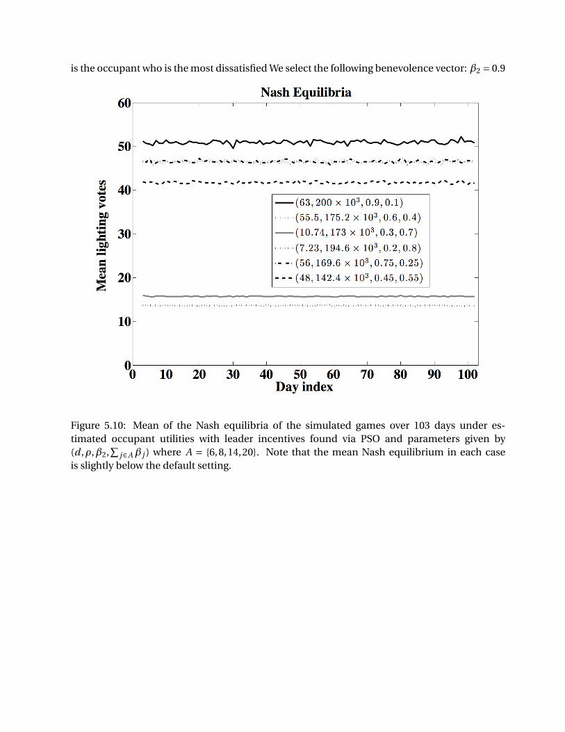
is the occupant who is the most dissatisfied We select the following benevolence vector: β2 = 0.9

Figure 5.10: Mean of the Nash equilibria of the simulated games over 103 days under es-timated occupant utilities with leader incentives found via PSO and parameters given by(d ,ρ,β2,

∑j∈Aβ j ) where A = 6,8,14,20. Note that the mean Nash equilibrium in each case

is slightly below the default setting.

Chapter 6

Conclusions

6.1 Summary

We have designed and implemented a social game for inducing building occupants to behave

in an energy efficient manner. We presented data and results pertaining to the game in which

occupants select their lighting preferences and win points depending on how far their vote is

from the baseline lighting setting and proportional to other occupants’ votes distances from

the baseline. As a result, the occupants are interacting in a competitive environment which

we model as a non-cooperative game. We show that we get significant savings as compared to

usage prior to the implementation of the social game. This savings is due to both a change in

the default setting as well as due to the incentives offered in the social game.

We described the experimental set-up which includes an online platform for the implemen-

tation of the social game as well as the use of a Lutron lighting system for precise control of the

lighting and HVAC setting. We have formulated the problem of estimating the occupant util-

ity functions as a convex optimization problem and estimated occupant utilities in a 20 player

social game. We simulated the game using the estimated utility functions and showed that our

model is a good predictor for occupant behavior.

By using the estimated utilities, we formulated and solved the building manager’s bi-level

44

optimization problem for the total points and default setting. Due to the large number of events

underlying the joint distribution across player states and non-convexities, we utilized a particle

swarm optimization method. We are exploring more efficient methods for solving for the opti-

mal points and default setting as well as implementing the current (d ,ρ) that we found through

PSO in our test bed.

The leader’s utility function contains a number of parameters such as c1,c2 and the benevo-

lence factor which represent how much utility or happiness the leader is willing to exchange for

savings. We are in the process of examining the impact of these factors on the leader savings as

well as the occupant satisfaction in practice. We are implementing surveys to collect additional

data about the occupants’ satisfaction which we plan to incorporate into our solution.

In addition, we did not include individual rationality constraints in the leader’s optimization

problem. It would be interesting to explore incorporating such a constraint in the optimization

problem where we consider the outside good to be the default setting. This problem is slightly

different than what is seen in the economics literature because the leader here has control over

the default setting, and thus, the outside good.

6.2 Future Work

Our platform also includes the ability to implement a social game for occupant plug-load con-

sumption. We are on the bring of a social game which will try to incentivize occupants to reduce

their plug-load consumption. Another interesting direction for future research that we are ex-

ploring is understanding the type (parameter) space of the occupants and how the Nash equi-

libria of the follower game depend on these parameters. Specificically it is interesting to take a

dynamical systems perspective and study parameter configurations leading to the desired Nash

equilibrium being structurally stable.

Furthermore, there are several ways in which we believe we can improve our estimate of

the utility functions of the occupants. We did not consider the environmental noise such as

variations in natural light. We instead used a heuristic to capture this variation by breaking the

day into intervals in which the natural light entering the office is most consistent. In addition,

we did not consider any information on the occupants’ schedules or location in the office with

respect to windows. We could incorporate these aspects into our estimation as priors on the

parameters of the occupants utility function or as a noise process in the estimated behavior

model.

Moreover, as to achieve better predictions we currently explore non linear regression models

for the occupants. We try to find appropriate Kernel functions as to improve our understanding

of human’s behavior model reacting to the Social Game and boost our daily predictions for the

office’s average implemented light and HVAC condition.

In addition, we want to improve our estimation techniques of the utility function parameters

in the case of a large scale implementation of the Social Game in whole building(s). In this case

we don’t want to optimize over a sampling subset of the data since the computational effort

would be increased as the Social Game will have a great many occupants. Our goal is to build an

optimization problem for the moment function of the distribution of the occupants parameter

θi .

List of symbols

Symbol Unit Meaning

βi - benevolence factor

c1 - scaling factor

c2 - scaling factor

d % default light setting

θi - utility’s function parameter

K kWh maximum consumption of the Lutron lighting system

ρ - points distributed by the building manager each day

x % implemented lighting setting

xb % baseline setting for lights

xi % occupant’s light vote

47

Bibliography

[1] M.H. Albadi and E.F. El-Saadany. A summary of demand response in electricity markets.

Electric Power Systems Research, 78(11):1989 – 1996, 2008.

[2] A. Aswani, N. Master, J. Taneja, V. Smith, A. Krioukov, D. Culler, and C. Tomlin. Identifying

models of HVAC systems using semi-parametric regression. In Proceedings of the American

Control Conference, 2012.

[3] Dimitri P Bertsekas. Nonlinear programming. Athena Scientific, 1999.

[4] Aaron Bestick, Lillian J Ratliff, Posu Yan, Ruzena Bajcsy, and S Shankar Sastry. An inverse

correlated equilibrium framework for utility learning in multiplayer, noncooperative set-

tings. In Proceedings of the 2nd ACM international conference on High confidence networked

systems, pages 9–16. ACM, 2013.

[5] Magnus Boman, Paul Davidsson, Nikolaos Skarmeas, Keith Clark, and Rune Gustavsson.

Energy saving and added customer value in intelligent buildings. In Third International

Conference on the Practical Application of Intelligent Agents and Multi-Agent Technology,

pages 505–517, 1998.

[6] Denis Bourgeois, Christoph Reinhart, and Iain Macdonald. Adding advanced behavioural

models in whole building energy simulation: A study on the total energy impact of manual

and automated lighting control. Energy and Buildings, 38(7):814 – 823, 2006. Special Issue

on Daylighting Buildings.

[7] Bradley Efron and Robert J Tibshirani. An introduction to the bootstrap, volume 57. CRC

press, 1994.

48

[8] Sjur D Flåm. Solving non-cooperative games by continuous subgradient projection meth-

ods. In System Modelling and Optimization, pages 115–123. Springer, 1990.

[9] N. Groot, B. De Schutter, and H. Hellendoorn. Reverse stackelberg games, part i: Basic

framework. In IEEE International Conference on Control Applications,, pages 421–426, Oct

2012.

[10] J. Kennedy and R. Eberhart. Particle swarm optimization. In Proceedings of the IEEE Inter-

national Conference on Neural Networks, volume 4, pages 1942–1948, Nov 1995.

[11] James Kennedy. Particle swarm optimization. In Encyclopedia of Machine Learning, pages

760–766. Springer, 2010.

[12] Arezou Keshavarz, Yang Wang, and Stephen Boyd. Imputing a convex objective function.

In IEEE International Symposium on Intelligent Control, pages 613–619. IEEE, 2011.

[13] M. Lee, O.Aslam, B. Foster, D. Kathan, J. Kwok, L. Medearis, R. Palmer, P. Sporborg, and

M. Tita. Assessment of demand response and advanced metering. Technical report, Federal

Energy Regulatory Commission, 2013.

[14] Tom Lovett, Elizabeth Gabe-Thomas, Sukumar Natarajan, Eamonn O’Neill, and Julian Pad-

get. ’just enough’ sensing to enliten: A preliminary demonstration of sensing strategy for

the ’energy literacy through an intelligent home energy advisor’ (enliten) project. In Pro-

ceedings of the Fourth International Conference on Future Energy Systems, pages 279–280,

New York, NY, USA, 2013. ACM.

[15] Y. Ma, G. Anderson, and F. Borrelli. A distributed predictive control approach to building

temperature regulation. In Proceedings of the American Control Conference, pages 2089–

2094. IEEE, 2011.

[16] J.L. Mathieu, M.E. Dyson, D.S. Callaway, and A. Rosenfeld. Using residential electric loads

for fast demand response: The potential resource and revenues, the costs, and policy rec-

ommendations. In ACEEE Summer Study on Energy Efficiency in Buildings, 2012.

[17] Johanna L Mathieu, Phillip N Price, Sila Kiliccote, and Mary Ann Piette. Quantifying

changes in building electricity use, with application to demand response. IEEE Transac-

tions on Smart Grid,, 2(3):507–518, 2011.

[18] JM McQuade. A system approach to high performance buildings. United Technologies

Corporation, Tech. Rep, 2009.

[19] Deepak Merugu, Balaji S Prabhakar, and NS Rama. An incentive mechanism for decon-

gesting the roads: A pilot program in bangalore. In Proceedings of ACM NetEcon Workshop,

2009.

[20] F. Oldewurtel, A. Parisio, C.N. Jones, M. Morari, D. Gyalistras, M. Gwerder, V. Stauch,

B. Lehmann, and K. Wirth. Energy efficient building climate control using stochastic model

predictive control and weather predictions. In Proceedings of the American Control Confer-

ence, pages 5100–5105, 2010.

[21] Lillian J. Ratliff, Samuel A. Burden, and S. Shankar Sastry. Characterization and computa-

tion of local nash equilibria in continuous games. In Proceedings of the 51st Annual Allerton

Conference on Communication, Control, and Computing, 2013.

[22] Lillian J. Ratliff, Samuel A. Burden, and S. Shankar Sastry. Generictiy and structural sta-

bility of non–degenerate differential nash equilibria. In Proceedings of the 2014 American

Controls Conference, 2014.

[23] Lillian J Ratliff, Roy Dong, Henrik Ohlsson, and S Shankar Sastry. Incentive design and

utility learning via energy disaggregation. In Proceedings of the 19th World Congress of the

International Federation of Automatic Control, 2014.

[24] M. Roozbehani, M. Dahleh, and S. Mitter. Dynamic pricing and stabilization of supply and

demand in modern electric power grids. In First IEEE International Conference on Smart

Grid Communications (SmartGridComm),, pages 543 –548, oct. 2010.

[25] J. B. Rosen. Existence and uniqueness of equilibrium points for concave n-person games.

Econometrica, 33(3):520, 1965.

[26] Alan Swenson. Lighting in commercial buildings. Technical report, U.S. Energy Infomation

Administration, 2009.

[27] Gerhard Venter and Jaroslaw Sobieszczanski-Sobieski. Particle swarm optimization. AIAA

journal, 41(8):1583–1589, 2003.