Social Investments, Informal Risk Sharing and Inequality∗

Attila Ambrus† Arun G. Chandrasekhar‡ Matt Elliott§

September 2014

Abstract

This paper investigates costly social investments, in the context of risk-sharing. Ex-tending the bargaining micro-foundations of Stole and Zwiebel (1996), we postulate thatthe benefits of risk-sharing are distributed according to the Myerson value. In particular,more centrally connected individuals receive a higher share of the surplus. Our mainfocus is comparing individual versus social incentives to establish relationships. If agentsin the community are homogenous, there is never underinvestment relative to the sociallyefficient benchmark. In contrast, there can be severe overinvestment. We find a noveltrade-off between efficiency and equality, and show that the most stable efficient networkis also the most unequal one. When there are multiple groups in a society, and incomes aremore correlated within groups, underinvestment across groups is possible and more cen-tral agents have better incentives to form across-group links. Using data from 75 Indianvillage networks, we provide empirical evidence consistent with our model’s predictions.We show that the comparative statics of network structure as economic environmentalparameters are changed are consistent with our theory, using a difference-in-differenceapproach looking at the risk-sharing network versus the friendship network.

1 Introduction

In the context of missing formal insurance markets, and limited access to lending and bor-rowing, incomes may be smoothed through informal risk sharing arrangements that utilizesocial connections and mitigate utility losses. A large theoretical and empirical literaturestudies this,1 but less attention has been paid to the network formation problem and thesocial investments that enable risk sharing. We study whether social investments are effi-cient. If not, is too much time allocated to maintaining relationships or too little? Moreover,do the forces pushing towards under and/or over investment generate inequality in societyeven when agents are ex-ante homogenous? And if so, does social inequality translate intofinancial inequality?

∗We thank the National Science Foundation, SES-1155302, for funding the research that collected the datawe use. We thank Nageeb Ali, Ben Golub, Willemien Kets, Cynthia Kinnan, Rachel Kranton, Peter Landryand Horacio Larreguy for helpful comments.†Department of Economics, Duke University; email: attila.ambrus@duke.edu‡Department of Economics, Stanford University and NBER; email: arungc@stanford.edu§Division of the Humanities and Social Sciences, California Institute of Technology; email: mel-

liott@hss.caltech.edu1An incomplete list of papers includes Rosenzweig (1988), Fafchamps (1992), Coate and Ravallion (1993),

Townsend (1994), Udry (1994), Ligon, Thomas and Worral (2000), Fafchamps and Gubert (2007), Angelucciand di Giorgi (2009).

1

Both underinvestment and overinvestment in social capital are conceivable. Two peopleestablishing a social connection to share risk gain access to a less stochastic income streamwhich might generate improved opportunities to share risk with their other connections.As these positive spillovers might not be fully taken into account when deciding whether toestablish the link, underinvestment can prevail. On the other hand, if more socially connectedindividuals receive a higher share of the surplus generated by risk sharing, that can lead tooverinvestment. Villagers may form links to redistribute the surplus towards themselves,rather than to increase the overall surplus generated. The empirical literature also suggeststhat both types of inefficiencies are possible, in different contexts. Austen-Smith and Fryer(2006) cites numerous references from sociology and anthropology, suggesting that members ofpoor communities allocate inefficiently large amounts of time to activities maintaining socialties, instead of productive activities. In contrast, Feigenberg et al. (2013) find evidence ina microfinance setting that it is relatively easy to experimentally intervene and create socialties among people that yield substantial benefits. One explanation for this finding is thatthere is underinvestment in social relationships.

It is important to study whether there is too little or too much investment into socialrelations, both to put related academic work (which often takes social connections to beexogenously given) into context, and to guide policy choices. Consider the example of micro-finance. If there is overinvestment, microfinance has a greater scope for efficiency savings interms of reducing people’s allocation of time into social investments. With underinvestment,however, it has more scope for smoothing incomes. If there is neither under nor overinvest-ment, it also tells us that informal risk sharing is working relatively well as a second-bestsolution. Understanding which regime applies can help anticipate policy implications andevaluate welfare impacts of interventions.

To explore efficiency and inequality, in this paper we consider a two-stage model ofnetwork-formation and risk-sharing, in a context in which agents with constant absolute riskaversion (CARA) utilities face uncertain endowment realizations. In the first stage, agentschoose with whom to form connections. Link formation is costly, as in Myerson (1991) andJackson and Wolinsky (1996). In the second stage connected agents commit to a risk-sharingarrangement that is contingent on future endowment realizations.2 We show that in ourCARA setting expected utilities are transferrable through state-independent transfers, andefficient risk-sharing arrangements on any network component are uniquely pinned down upto these transfers. The latter determine the allocation of surplus among agents. To keep themodel tractable, we abstract away from the issues of how to enforce risk-sharing agreements.3

We assume that the social surplus generated by efficient risk-sharing arrangements isdistributed among the agents according to the Myerson value, a network-specific version ofthe Shapley value.4 Our motivation here comes from two sources. First, if the surplus di-vision is chosen in a centralized manner, then it has normative appeal on the grounds offairness: two agents benefit equally from a social relationship between them, and receivebenefits proportional to their average contributions to total surplus (from establishing costly

2Although we consider a model in which there is perfect risk sharing of income, we could easily extend themodel so that some income is perfectly observed, some income is private and there is perfect risk sharing ofobservable income and no risk sharing of unobservable income. This would be consistent with the theoreticalpredictions of Cole and Kocherlakota (2001) and the empirical findings of Kinnan (2011). In the CARAutilities setting such unobserved income outside the scope of the risk-sharing arrangement does not affect ourresults.

3See Ambrus et al. (2014) for an investigation of such issues.4For other investigations of the division of surplus in social networks, see Calvo-Armengol (2001, 2003),

Corominas-Bosch (2004), Manea (2011), and Kets et al. (2011).

2

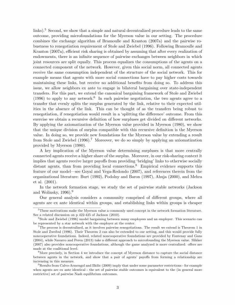
links).5 Second, we show that a simple and natural decentralized procedure leads to the sameoutcome, providing microfoundations for the Myerson value in our setting. The procedurecombines the exchange algorithm of Bramoulle and Kranton (2007a) and the pairwise ro-bustness to renegotiation requirement of Stole and Zwiebel (1996). Following Bramoulle andKranton (2007a), efficient risk sharing is obtained by assuming that after every realization ofendowments, there is an infinite sequence of pairwise exchanges between neighbors in whichjoint resources are split equally. This process equalizes the consumptions of the agents on aconnected component of the network. However, given this social norm, all connected agentsreceive the same consumption independent of the structure of the social network. This forexample means that agents with more social connections have to pay higher costs towardsmaintaining these links, but receive no additional benefits from doing so. To address thisissue, we allow neighbors ex ante to engage in bilateral bargaining over state-independenttransfers. For this part, we extend the canonical bargaining framework of Stole and Zwiebel(1996) to apply to any network.6 In each pairwise negotiation, the two agents agree to atransfer that evenly splits the surplus generated by the link, relative to their expected util-ities in the absence of the link. This can be thought of as the transfers being robust torenegotiation, if renegotiation would result in a ‘splitting the difference’ outcome. From thisexercise we obtain a recursive definition of how surpluses get divided on different networks.By applying the axiomatization of the Myerson value provided in Myerson (1980), we showthat the unique division of surplus compatible with this recursive definition is the Myersonvalue. In doing so, we provide new foundations for the Myerson value by extending a resultfrom Stole and Zwiebel (1996).7 Moreover, we do so simply by applying an axiomatizationprovided by Myerson (1980).

A key implication of the Myerson value determining surpluses is that more centrallyconnected agents receive a higher share of the surplus. Moreover, in our risk-sharing context itimplies that agents receive larger payoffs from providing ‘bridging’ links to otherwise sociallydistant agents, than from providing local connections.8 Empirical evidence supports thisfeature of our model—see Goyal and Vega-Redondo (2007), and references therein from theorganizational literature: Burt (1992), Podolny and Baron (1997), Ahuja (2000), and Mehraet al. (2001).

In the network formation stage, we study the set of pairwise stable networks (Jacksonand Wolinsky, 1996).9

Our general analysis considers a community comprised of different groups, where allagents are ex ante identical within groups, and establishing links within groups is cheaper

5These motivations make the Myerson value a commonly used concept in the network formation literature.See a related discussion on p 422-425 of Jackson (2010).

6Stole and Zwiebel (1996) model bargaining between many employees and an employer. This scenario canbe represented by a star network with the employer at the center.

7The process is decentralized, as it involves pairwise renegotiations. The result we extend is Theorem 1 inStole and Zweibul (1996). Their Theorem 2 can also be extended to our setting, and this would provide fullynoncooperative foundations. Indeed, related noncooperative foundations are provided by Fontenay and Gans(2004), while Navarro and Perea (2013) take a different approach to microfounding the Myerson value. Slikker(2007) also provides noncooperative foundations, although the game analyzed is more centralized: offers aremade at the coalitional level.

8More precisely, in Section 4 we introduce the concept of Myerson distance to capture the social distancebetween agents in the network, and show that a pair of agents’ payoffs from forming a relationship areincreasing in this measure.

9Results from Calvo-Armengol and Ilkilic (2009) imply that under some parameter restrictions - for examplewhen agents are ex ante identical - the set of pairwise stable outcomes is equivalent to the (in general morerestrictive) set of pairwise Nash equilibrium outcomes.

3

than across groups. We also assume that the endowment realizations of agents within groupsare more positively correlated than across groups. Groups can represent different ethnicgroups or castes in a given village, or different villages. The core results show that therecan only be overinvestment within groups10 but no underinvestment, whereas, across groupsunderinvestment is likely to be the main concern.

To see the intuition about overinvestment within groups, we first consider the case of ho-mogenous agents, that is when there is only one group. Using the inclusion-exclusion principlefrom combinatorics, we provide a complete characterization of stable networks. We show thatin this case there can never be underinvestment in social connections, as agents establishingan essential link (connecting two otherwise unconnected components of the network) alwaysreceive a benefit exactly equal to the social value of the link. However, overinvestment, in theform of redundant links, is possible, and becomes widespread as the cost of link formationdecrease. We also find a trade-off between efficiency and equality. Among all possible efficientnetwork structures, we find that the most stable (for the largest set of parameter values) isthe star, which also results in the most unequal division of surplus. The intuition is that thatthe star network minimizes the incentives of peripheral agents to establish redundant links.Conversely, the least stable efficient network entails the most equal division of surplus amongall stable networks. Although agents are ex-ante identical, efficiency considerations push thestructure of social connections towards asymmetric outcomes that elevate certain individuals.Socially central individuals emerge endogenously from risk-sharing considerations alone.11

Turning attention to the case of multiple groups, we find that across group underinvest-ment becomes an issue when the cost of maintaining links across groups is sufficiently high.12

The reason is that the agents who establish the first connection across groups receive lessthan the total surplus generated by the link, providing positive externalities for peers intheir groups. This gap between private and social benefits is smaller for agents located morecentrally in their own group, providing a second force for some agents within a group tobe more central. For two groups, we show that the most stable efficient network structureinvolve “stars” within groups, connected by their centers, and we establish a weaker formof this result for more than two groups. This reinforces the trade-off between efficiency andequality, in the many groups context.

Using data from 75 Indian villages, we provide some supporting evidence for our model.We split the villagers into two groups, by caste.13 From the theoretical analysis, risk sharinglinks are most valuable when they bridge otherwise unconnected components. And when alink does not provide such a bridge, its value depends on how far apart, suitably defined,the agents would otherwise be on the social network. We call this distance between a pairof agents their Myerson distance. Our theory predicts that there is an upper bound on theMyerson distance between any two unconnected agents within the same group, beyond whichthe pair of agents would have a profitable deviation by forming a link. In addition we predictthat there will be inquality is social positions and that more central agents within their groupwill form across group links. However, there are many alternative stories consistent with these

10This is subject to a regularity condition that it is socially valuable for two agents from the same caste, ifthey would otherwise be isolated, to form a link and share risk together.

11In certain settings, over time, these central individuals could also establish more formal financial institu-tions, creating more entrenched inequality.

12While across group overinvestment remains possible, when across group link costs are relatively high, themain concern is underinvestment.

13There is an extensive literature that examines caste as a main social unit where risk sharing takes place(Townsend (1994), Munshi and Rosenzweig (2009), and Mazzocco and Saini (2012)).

4

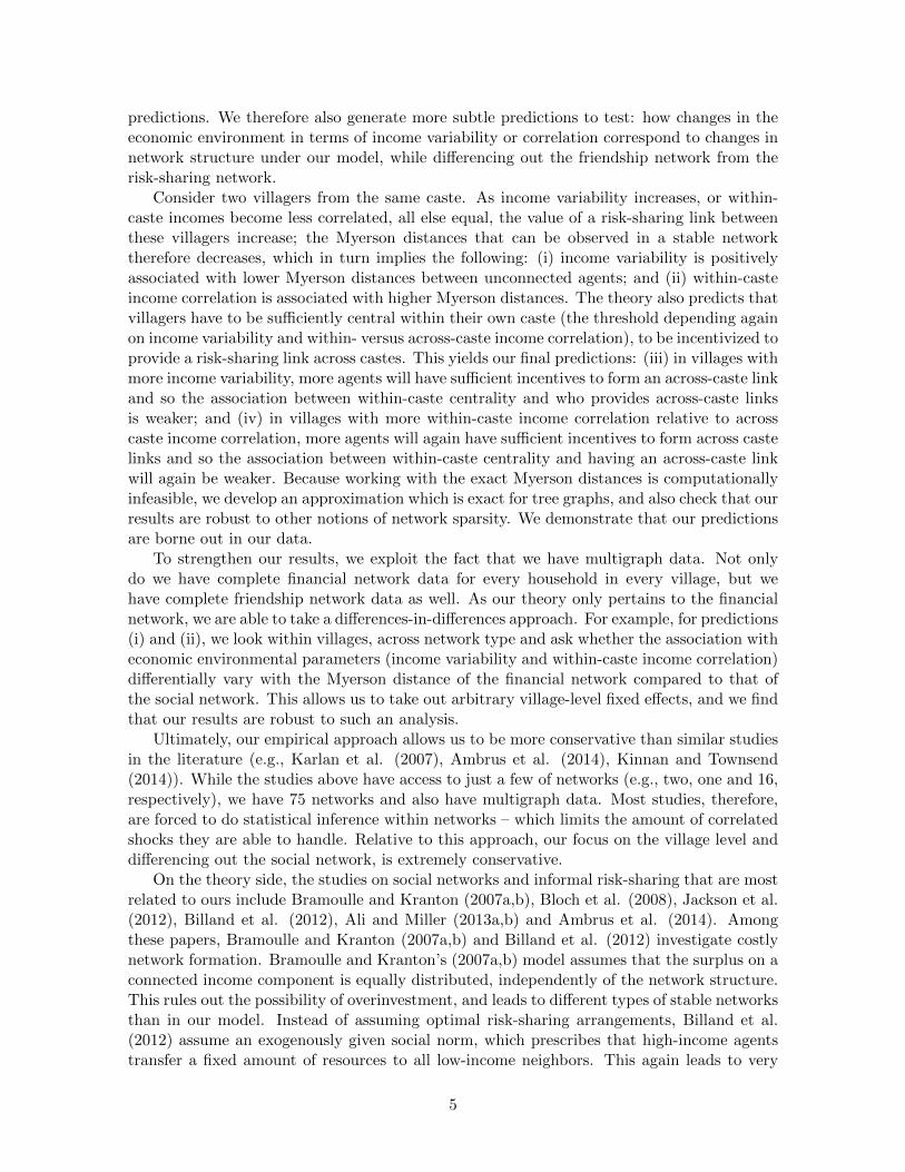
predictions. We therefore also generate more subtle predictions to test: how changes in theeconomic environment in terms of income variability or correlation correspond to changes innetwork structure under our model, while differencing out the friendship network from therisk-sharing network.

Consider two villagers from the same caste. As income variability increases, or within-caste incomes become less correlated, all else equal, the value of a risk-sharing link betweenthese villagers increase; the Myerson distances that can be observed in a stable networktherefore decreases, which in turn implies the following: (i) income variability is positivelyassociated with lower Myerson distances between unconnected agents; and (ii) within-casteincome correlation is associated with higher Myerson distances. The theory also predicts thatvillagers have to be sufficiently central within their own caste (the threshold depending againon income variability and within- versus across-caste income correlation), to be incentivized toprovide a risk-sharing link across castes. This yields our final predictions: (iii) in villages withmore income variability, more agents will have sufficient incentives to form an across-caste linkand so the association between within-caste centrality and who provides across-caste linksis weaker; and (iv) in villages with more within-caste income correlation relative to acrosscaste income correlation, more agents will again have sufficient incentives to form across castelinks and so the association between within-caste centrality and having an across-caste linkwill again be weaker. Because working with the exact Myerson distances is computationallyinfeasible, we develop an approximation which is exact for tree graphs, and also check that ourresults are robust to other notions of network sparsity. We demonstrate that our predictionsare borne out in our data.

To strengthen our results, we exploit the fact that we have multigraph data. Not onlydo we have complete financial network data for every household in every village, but wehave complete friendship network data as well. As our theory only pertains to the financialnetwork, we are able to take a differences-in-differences approach. For example, for predictions(i) and (ii), we look within villages, across network type and ask whether the association witheconomic environmental parameters (income variability and within-caste income correlation)differentially vary with the Myerson distance of the financial network compared to that ofthe social network. This allows us to take out arbitrary village-level fixed effects, and we findthat our results are robust to such an analysis.

Ultimately, our empirical approach allows us to be more conservative than similar studiesin the literature (e.g., Karlan et al. (2007), Ambrus et al. (2014), Kinnan and Townsend(2014)). While the studies above have access to just a few of networks (e.g., two, one and 16,respectively), we have 75 networks and also have multigraph data. Most studies, therefore,are forced to do statistical inference within networks – which limits the amount of correlatedshocks they are able to handle. Relative to this approach, our focus on the village level anddifferencing out the social network, is extremely conservative.

On the theory side, the studies on social networks and informal risk-sharing that are mostrelated to ours include Bramoulle and Kranton (2007a,b), Bloch et al. (2008), Jackson et al.(2012), Billand et al. (2012), Ali and Miller (2013a,b) and Ambrus et al. (2014). Amongthese papers, Bramoulle and Kranton (2007a,b) and Billand et al. (2012) investigate costlynetwork formation. Bramoulle and Kranton’s (2007a,b) model assumes that the surplus on aconnected income component is equally distributed, independently of the network structure.This rules out the possibility of overinvestment, and leads to different types of stable networksthan in our model. Instead of assuming optimal risk-sharing arrangements, Billand et al.(2012) assume an exogenously given social norm, which prescribes that high-income agentstransfer a fixed amount of resources to all low-income neighbors. This again leads to very

5

different predictions regarding the types of networks that form in equilibrium.More generally, network formation problems are important. Establishing and maintaining

social connections (relationships) is costly, in terms of time and other resources. However,on top of direct consumption utility, such links can yield many economic benefits. Papersstudying formation in different contexts include Jackson and Wolinsky (1996), Bala andGoyal (2000), Kranton and Minehart (2001), Hojman and Szeidl (2008), and Elliott (2013).Notable in this literature is a lack empirical work, which can be attributed to a numberof innate difficulties that taking these models to data presents. One common problem isa multiplicity of stable networks. But perhaps most important, is that the networks inquestion can only very rarely be partitioned into a sizeable number of separate networks thatcan reasonably be treated as independent. Since predictions are often at the level of theoverall network structure, this makes testing extremely challenging. Our many observationsof social networks that are relatively independent of each other coupled with our approachto circumventing data limitations, allow us to provide a first step towards testing predictionsbased on the overall network structure. And although we study a quite specific networkformation problem tailored to risk-sharing in villages, the general structure of our problemis relevant other applications.14

The remainder of the paper is organized as follows. Section 2 describes risk sharing ona fixed network. In Section 3 we introduce a game of network formation with costly linkformation. We focus on network formation within a single group first in Section 4 and thenturn to the formation of across-group links in Section 5. We empirically test predictions ofour model in the data in Section 6. Section 7 concludes.

2 Preliminaries: Risk-Sharing on a Fixed Network

We consider an economy in which agents face stochastic income realizations, but can insureagainst this uncertainty through redistributions made over the network of social connections.Ultimately we are interested in investigating endogenous network formation. However, inorder to define a noncooperative game of investing into social connections, first we will specifythe risk-sharing arrangement that prevails for any given network.

The social structureWe denote the set of agents in our model by N, and assume that they are partitioned into

a set of groups M. We let G : N→M be a function that assigns each agent to a group; i.e.,if G(i) = g then agent i is in group g. One interpretation of the group partitioning is thatN represents individuals in a village, and the groups correspond to different castes. Anotherpossible interpretation is that N represents individuals in a larger geographic region (such asa district or subdistrict), and groups correspond to different villages in the region.

The social network is represented by an undirected graph L on the set of nodes corre-sponding to agents in N such that lij ∈ L is interpreted as a link exists between agents iand j. The social network influences both the set of feasible risk-sharing arrangements andthe distribution of surplus from risk sharing, as described below. There can be links bothbetween agents in the same group and between agents in different groups.

14For a different more specific and more removed application, suppose researches can collaborate on aproject. Each researcher brings something heterogenous and positive to the value of the collaboration so thatthe value of the collaboration is increasing in the set of agents involved. Collaboration is only possible whenamong agents who are directly connected to another collaborator, and surplus is split according to the Myersonvalue (as in our work, motivated by robustness to renegotiations). Such a setting fits into our framework.

6

We will refer to N(i;L) ≡ j : lij ∈ L ⊂ N as agent i’s neighbors. An agent’s neighborscan be partitioned according to the groups they belong to. Let Ng(i;L) be i’s neighborson network L from group g. We will sometimes refer to subsets of agents S ⊆ N anddenote the subgraphs they generated by L(S) ≡ lij ∈ L : i, j ∈ S. A subset of agentsS ⊆ N is path connected on L if, for each i ∈ S and each j ∈ S, there exists a sequence ofagents (a path) i, k, k′, . . . , k′′, j such that every pair of adjacent agents in the sequence islinked. For any network there is a unique partition of N such that there are no links betweenagents in different partitions but all agents within a partition are path connected. We referto the cells of this partition as network components. The shortest path between two pathconnected agents is the path with the shortest sequence of agents. The diameter of a networkcomponent, d(C), is the maximum length of the shortest path between any two agents in C.A network component is a tree when there is a unique path between any two agents in thecomponent. The degree centrality of an agent is simply the number of neighbors he has (i.e.the cardinality of N(i)).

Incomes and ConsumptionAgents in N face uncertain income realizations. For tractability, we assume that incomes

are jointly normally distributed, with expected value µ and variance σ2 for each agent.15 Weassume that the correlation coefficient between the incomes of any two agents within the samegroup is ρw, while between incomes of any two agents not in the same group is ρa < ρw.16

That is, we assume that incomes are more positively correlated within groups than acrossgroups, so that all else equal, social connections across groups have a higher potential forrisk-sharing.

Although we introduce the possibility of correlated incomes in a fairly stylized way, ourpaper is one of the first to permit differentially correlated incomes between different groups.Such correlations are central to the effectiveness of risk-sharing arrangements, as shown below.

We refer to possible realizations of the vector of incomes as states, and denote a genericstate by ω. We let yi(ω) denote the income realization of agent i in state ω.

Agents can redistribute realized incomes, as described below; hence their consumptionlevels can differ from their realized incomes. We assume that all agents have constant absoluterisk aversion (CARA) utility functions:

u(ci) = − 1

λe−λci ,

where ci is agent i’s consumption and λ > 0 is the coefficient of absolute risk aversion.

Efficient Risk-Sharing AgreementsWe assume that income can only be directly shared between agents i, j ∈ N if they

are connected, i.e. lij ∈ L. However, through a sequence of bilateral transfers betweenconnected agents, incomes can be arbitrarily redistributed within any component of thenetwork. As the main focus of our paper is network formation, to keep the model tractablewe abstract away from enforcement constraints, and analogously to Bramoulle and Kranton(2007a, 2007b), we assume that all neighboring agents share risk efficiently, which in turn

15This specification implies that we cannot impose a lower bound on the set of feasible consumption levels.As we show below, our framework readily generalizes to arbitrary income distributions, but the assumptionof normally distributed shocks simplifies the analysis considerably.

16It is well-known that for a vector of random variables not all combinations of correlations are possible. Weimplicitly assume that our parameters are such that the resulting correlation matrix is positive semidefinite.

7

leads to ex ante Pareto-efficient risk sharing at the level of each connected component.17

While in practice risk sharing is imperfect, prefect risk sharing provides a useful benchmark.It is also straightforward to extend the model so that some income is publicly observed andperfectly shared while remaining income is privately observed and never shared. Results arevery similar for this more general setting.18

Formally, a risk-sharing agreement specifies a consumption vector c for every state, in away that

∑i∈C ci(ω) ≤

∑i∈C yi(ω) for every state ω and network component C.

In Proposition 1 below we show that the CARA utilities framework has the convenientproperty that expected utilities are transferrable, in the sense defined by Bergstrom andVarian (1985). Moreover, ex ante Pareto efficiency is equivalent to minimizing the sum ofvariances, and it is achieved by agreements that at every state split the sum of the incomesat each network component equally among members and then adjust these shares by state-independent transfers. The latter determine the division of the surplus created by the risk-sharing agreement. We emphasize that this result does not require any assumption on thedistribution of incomes, only that agents have CARA utilities.

Proposition 1 For CARA utility functions certainty equivalent units of consumption aretransferrable across agents, and if L(S) is a network component the Pareto frontier of exante risk-sharing agreements among agents in S is represented by a simplex in the space ofcertainty equivalent consumption. The ex ante Pareto-efficient risk-sharing agreements foragents in S are those that satisfy:

min∑i∈S

Var(ci) subject to∑i∈Sci(ω) =

∑i∈Syi(ω) for every state ω,

and they are comprised of agreements of the form

ci(ω) =1

|S|∑k∈S

yk(ω) + τi for every i ∈ S and state ω.

Proof. See Appendix A.

The first statement in Proposition 1 can be established by showing that, with CARAutilities, the certainty equivalent consumption for a lottery is independent of the consump-tion level. The results on the Pareto-efficient risk-sharing arrangements can be obtained byapplying the classic Borch rule (Borch (1962), Wilson (1968)) and algebraically manipulatingthe resulting conditions.

Proposition 1 implies that the total surplus generated by an efficient risk-sharing arrange-ment is an increasing function of the reduction in the sum of consumption variances. Forgeneral distribution of shocks, this function can be complicated. However, when shocks arejointly normally distributed, then ci = 1

|S|∑

k∈S yk + τi is also normally distributed, and

17For a model of informal insurance in social networks in which the set of feasible agreements are constrainedby enforceability requirements, but in which the social network is exogenously given, see Ambrus et al. (2012).

18Kinnan (2011) finds evidence that hidden income can explain imperfect risk sharing in Thai villagesrelative to the enforceability and moral hazard problems we are abstracting from. Cole and Kocherlakota(2001) show that when individuals can privately store income, state-contingent transfers are not possible andrisk sharing is limited to borrowing and lending.

8

E(u(ci)) = E(ci) − λ2 Var(ci).

19 Hence in this case the total social surplus generated by ef-ficient risk-sharing agreements is proportional to the total consumption variance reduction.This greatly simplifies computing surpluses in the analysis below.

We use TS(L) to denote the expected total surplus generated by an ex ante Pareto efficientrisk-sharing agreement on network L, relative to agents consuming in autarky.

Division of SurplusWe assume that agents on a connected component divide the total surplus created by

the risk-sharing arrangement according to the Myerson value (Myerson (1977), (1980)). TheMyerson value is a cooperative solution concept defined in transferable utility environments,that is a network-specific version of the Shapley value. The basic idea behind it is the sameas for the Shapley value. For any order of arrivals of players, the incremental contributionof an agent to the total surplus can be derived as the difference between the total surplusesgenerated by the subgraph of L defined by the given agent and those who arrived earlier,and by the subgraph that is defined by only those agents who arrived earlier. It is easy tosee that, for any order of arrivals, this way the total surplus generated by L gets exactlyallocated to the set of all agents. The Myerson value then allocates the average incrementalcontribution of a player to the total surplus, taken over all possible orders (permutations) ofplayers, as the player’s share of the total surplus. So agent i’s Myerson value is:20

MVi(L) ≡∑S⊆N

(|S| − 1)!(n− |S|)!n!

(TS(L(S))− TS(L(S/i))

).

Our motivation for using the Myerson value is twofold. First, if agents on a connectedcomponent decide on the division of the surplus in a centralized manner, the Myerson valueis selected based on normative considerations: the benefits received by an agent from theagreement should be equal to the average contribution of the agent to the social surplus.As shown in Myerson (1980), it is also implied by two very basic axioms: efficiency at thecomponent level, and the requirement that the marginal benefit of a link is the same for theconnecting agents, labeled as balanced contributions. Second, as we show below, a simpledecentralized procedure involving bilateral transactions also selects the Myerson value.

To start with, consider a procedure proposed in Bramoulle and Kranton (2007a): afterthe realization of endowments, neighboring agents have repeated meetings with each other, inan arbitrary order, and each time they equalize their incomes. As shown in the above paper,such a procedure leads to splitting the total endowment at any component of the networkequally among agents in the component. We increment this procedure with an ex ante stage,in which neighboring agents make bilateral agreements on ex ante transfers that are stateindependent and not subject to ex post redistribution. Analogously to Stole and Zwiebel(1996), we require these transfers to be renegotiation proof.

Formally, for network L, let ui(L) be i’s expected payoff ex ante (before incomes arerealized). We assume that for every lij ∈ L, agents i and j meet to negotiate a transfer

19See for example Arrow (1965).20Our assumption that there is perfect risk sharing among path connected agents ensures that a coalition of

path connected agents generates the same surplus regardless of the exact network structure connecting them.This means that we are in the communication game world originally envisaged by Myerson. We do not requirethe generalization of the Myerson value to network games proposed in Jackson and Wolinshy (1996), whichsomewhat confusingly is also commonly referred to as the Myerson value. Jackson (2006) critiques the gener-alization of the Myerson value on the grounds that the allocation is insensitive to heterogeneties in people’ssurplus generating capabilities that are captured by alternative, unformed networks. These heterogeneitiesare not possible in communication games.

9

before the endowments realize. We let each agent have the option of holding up the otherby deleting the link, and then negotiating its reformation. The network of social connectionsthat have already formed, provides an upper bound on the set of relationships that can beused for the purposes of risk sharing, so new links cannot be formed, but existing links canbe deleted and reformed. Implicitly, it takes a long time to establish a relationship, but onceformed that relationship can be dissolved and possibly reformed much faster. We supposethat when a link is reformed the agents ‘split the difference’ and benefit equally from thelink. Robustness to these renegotiations then requires that, at the margin, each formed linkbenefits both agents equally. Of course, in order to calculate what agents i and j wouldreceive in the network without the link lij , we have to consider what would happen if linkswere renegotiated in the network without lij and so on. The result is a recursive system ofequations. The value of the link is only directly pinned down when it is the only link for bothagents, and without the link both agents receive their autarky outcomes. Iterating, we cannow consider networks with two links, and so on. At each stage of this recursion we requirethat for each link lij ∈ L, the incremental benefit provided by the link is split equally betweenagents i and j. Following the terminology of Stole and Zwiebel (1996), we label risk-sharingarrangements satisfying the resulting criterion as robust to renegotiation.

Formally, for any network L, let U(L) be the set of mappings from all subnetworks of Lto RN , representing payoff vectors to agents for different network realizations. We refer toelements of U(L) as contingent payoff schemes given L. For a contingent payoff scheme u,let ui(L

′) denote the payoff of agent i given L′ ⊆ L. Lastly, for ease of exposition, we useL− lij instead of L\lij for the network obtained from L by deleting link lij .

Definition 2 For any network L, the payoff vector (u1, ..., uN ) is robust to renegotiation ifthere is a contingent payoff scheme u given L such that ui = ui(L) for every i ∈ N and:

(i) ui(L′)− ui(L′ − lij) = uj(L

′)− uj(L′ − lij) for every i,j ∈ N and L′ ⊆ L;(ii)

∑i∈N ui(L

′) = TS(L′) for every L′ ⊆ L.

Below we show that the requirement of robustness to split-the-difference renegotiationimplies all agents must receive their Myerson values.

Proposition 3 For any network L, there is a unique vector of payoffs that is robust torenegotiation and at this outcome all agents receive their Myerson Values: ui(L) = MVi(L).

Proof. We will use the axiomatization of the Myerson value established in Myerson (1980).21

This axiomatization states that there exists a unique payoff division rule satisfying that (i)any link benefits the two connecting agents equally; and (ii) the outcome is efficient at thecomponent level. Formally, these requirements are equivalent to properties (i) and (ii) indefinition 2. So a payoff vector is robust to renegotiation if and only if it corresponds to theMyerson value. Since the Myerson value is unique, there is a also a unique payoff vector thatis robust to renegotiation.

21An assumption made by Myerson when defining the Myerson value is that the surplus generated by aconnected component is independent of the network structure within the component. Networks are viewed ascommunication structures. Although the Myerson value was redefined more generally in Jackson and Wolinsky(1996), as we apply Myerson’s axiomatization it is important that our setting satisfies the communicationstructure assumption.

10

Proposition 2 is a direct implication of Myerson’s axiomatization of the value. A specialcase of Proposition 2 is Theorem 1 of Stole and Zwiebel (1996), which restrict attention toa star network. Our contribution is to point out that the connection between robustness torenegotiation and the Myerson value applies across all networks.

3 Investing in Social Relationships

In this section we first formally introduce a game of network formation in which establishinglinks is costly, and define the concepts of efficient networks and different types of inefficienciesin network formation.

We consider a two-period model in which in period 1 all agents simultaneously choosewhich other agents they would like to form links with, and in period 2 agents agree upon theex ante Pareto efficient risk-sharing agreement specified in the previous section (i.e., the totalsurplus from risk-sharing is distributed according to the Myerson value), whichever networkforms in the first period.22

Formally, in period 1, we consider a network formation game along the lines of Myerson(1991): all agents simultaneously choose a subset of the other agents, indicating who theywould like to form links (relationships) with. A link is formed between two agents if and onlyif they both want to form it – i.e. if both agents select each other. When agent i forms alink, he pays a cost κw > 0 if the link is with someone in the same group and κa > κw ifthe link is with someone from a different group. This specification assumes that two agentsforming a link have to pay the same cost for establishing the link. However, all of our resultsbelow would remain valid if we allowed the agents to share the total costs of establishing alink arbitrarily (namely if we allowed the agents in the first period not only indicating whothey would like to establish links with, but also propose a division of the costs of establishingeach link; a link would then only form if both agents indicate each other and they proposethe same split of the cost). This is because for any link, the Myerson value rewards thetwo agents establishing the link symmetrically. Hence the agents can find a split of the linkformation cost such that establishing the link is profitable for both of them if only if it isprofitable for both of them to form the link with an equal split of the cost. For this reasonwe stick with the simpler model with exogenously given costs.

The collection of links formed in period 1 becomes social network L.Normalizing the utility from autarchy to 0, agent i’s net payoff if network L forms is:

Ui(L) = MVi(L)− |NG(i)(i;L)|κw −(|N(i;L)| − |NG(i)(i;L)|

)κa.

The solution concept we apply to the simultaneous move game described above is pairwisestability. A network L is pairwise stable with respect to payoff functions ui(L)i∈N if andonly if for all i, j ∈ N , (i) if lij ∈ L then ui(L)−ui(L/lij) ≥ 0 and uj(L)−uj(L/lij) ≥ 0;and (ii) if lij /∈ L then ui(L ∪ lij) − ui(L) > 0 implies uj(L ∪ lij) − uj(L) < 0. In words,pairwise stability requires that no two players can both strictly benefit by establishing anextra link with each other, and no player can benefit by unilaterally deleting one of his links.

From now on we refer to pairwise stable networks simply as equilibrium networks. Ex-istence of a pairwise stable networks in our model follows from a result in Jackson (2003),

22For a complementary treatment of network formation when surplus is split according to the MyersonValue, see Pin (2011).

11

stating that whenever payoffs in a simultaneous-move network formation game are determinedbased on the Myerson value, there exists a pairwise stable network.

Proposition 4 (Jackson, 2003) There exists an equilibrium in the game of network for-mation.

A network L is efficient when there is no other network L′ and no risk sharing agreementon L′ that can make everyone at least as well off as they were on L and someone strictly betteroff. Let |Lw| be the number of within group links and let |La| be the number of across grouplinks. As expected utility is transferable in certainty equivalent units, efficient networks mustmaximize the net total surplus NTS(L):

NTS(L) ≡ CE(

∆ Var(L, ∅))− 2|Lw|κw − 2|La|κa, (1)

where, for L′ ⊂ L, ∆ Var(L,L′) is the additional variance reduction obtained by efficient risksharing on network L instead of L′, and CE(·) denotes the certainty equivalent value of avariance reduction.

Clearly two necessary conditions for a network to be efficient are that the removal of aset of links does not increase NTS(L) and the addition of a set of links does not increaseNTS(L). If there exists a set of links, the removal of which increases NTS(L) we will saythere is overinvestment inefficiency. If there exists a set of links the addition of which increasesNTS(L) we will say there is underinvestment inefficiency.23

We will say that a link lij is essential if after its removal i and j are no longer pathconnected.

Remark 5 Preventing overinvestment requires that all links are essential. Additional linkscreate no social surplus and are costly. In all efficient networks, every component musttherefore be a tree.

In most of the analysis below we focus on investigating the relationship between equilib-rium networks and efficient networks.

4 Local Network Formation

In this section we assume thatm = 1, that is agents are ex ante symmetric, and any differencesin their outcomes stem from their equilibrium positions on the social network. This will laythe foundations for the more general case considered in the next section.

The social value of a non-essential link is 0. We begin the analysis by characterizing thesocial value of an essential link. As shown in the previous subsection, the social value of a linkis proportional to the reduction it implies, through a Pareto efficient risk-sharing agreement,in the sum of the consumption variances. Let L(S1) and L(S2) be the network componentsof agent i and agent j on network L/lij, and let |S1| = s1 and |S2| = s2. Then the sum

23Note that these definitions are not mutually exclusive (there can be both underinvestment and overin-vestment inefficiency) or collectively exhaustive (inefficient networks can have neither underinvestment noroverinvestment inefficiency if an increase in net total surplus is possible by the simultaneous addition andremoval of edges).

12

of consumption variances on L(S1) and L(S2), assuming Pareto-efficient risk sharing, ares1+s1(s1−1)ρw

s1σ2 and s2+s2(s2−1)ρw

s2σ2, respectively. Once S1 and S2 are connected through lij ,

the sum of consumption variances on L(S1 ∪ S2) becomes s1+s2+(s1+s2)(s1+s2−1)ρws1+s2

σ2. Thisimplies that the consumption variance reduction induced by the link lij is ∆ Var(L∪lij, L) =(1− ρw)σ2. This means that the variance reduction, and therefore the surplus created by anessential link, in case of homogenous agents, is independent of the sizes of the componentsthe essential link connects. Intuitively, an increase in the size of one of the components,say s1, has two effects. On the one hand it increases the consumption variance reduction foragents S2 when they get linked to agents S1, as agents in the latter component can spread theincome risk from agents S2 more effectively. On the other hand it decreases the consumptionvariance reduction of agents S1 when they get linked to agents S2, as the increase in s1

implies that risk-sharing is better on S1 already. What the above formula shows is that forhomogenous agents these two effects perfectly cancel each other out.

This implies that it is particularly simple to determine the gross surplus created by net-work L. Let f(L) be the number of network components on L. Then:

CE(

∆ Var(L, ∅))

= (N − f(L))λ

2(1− ρw)σ2.

Since the surplus created by any essential link is V ≡ λ2 (1− ρw)σ2, total gross surplus is

equal to the latter constant times the number of network component reductions relative tothe empty network.

Next we investigate private incentives for link formation. Recall that the share of thesurplus created by risk-sharing allocated to an agent i is equal to the average incrementalsurplus created by adding him to the network, over all possible orders of arrival of players.Every link an agent has result in component reduction of 1 or no component reduction wheni is added. The link lij will reduce the number of components in the graph by one when i isadded, if and only if j has already been added and there is no other path between i and j.If there is another path between i and j, or j has not been added yet, then the link lij willnot result in any component reduction when i is added. Suppose agents S have been addedbefore i for a given permutation of arrival orders. As before we let L(S) ⊆ L be the subgraphof L such that lij ∈ L(S) if and only if lij ∈ L, i ∈ S and j ∈ S. If j 6∈ S, then the link lijis not formed when i is added and so i receives no benefit from it. If j ∈ S then lij reducesthe number of components present in the graph by 1 if there is no other path from i to j onL(S∪ i) and reduces the number of components in the graph by zero otherwise. The link lijis valuable to i when added if and only if it is essential on the graph L(S ∪ i).

Remark 6 Let Le(S∪ i) ⊆ L(S∪ i) be the set of essential links on L(S∪ i). The incrementalsurplus generated when i is added is proportional to the number of essential links i has onL(S ∪ i). In other words:

CE(

∆ Var(L(S ∪ i), L(S)))

=∣∣∣L(i) ∩ Le(S ∪ i)

∣∣∣ · V.We now characterize the set of pairwise stable networks. Some additional terminology

will be helpful. A minimal path between i and j is any path between i and j such that noother path between i and j is a subsequence. If there are K minimal paths between i and jon the network L, we let P(i, j, L) = P1(i, j, L), . . . , PK(i, j, L) be the set of these paths.

13

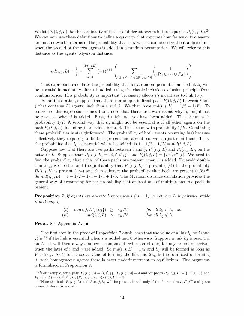
We let |Pk(i, j, L)| be the cardinality of the set of different agents in the sequence Pk(i, j, L).24

We can now use these definitions to define a quantity that captures how far away two agentsare on a network in terms of the probability that they will be connected without a direct linkwhen the second of the two agents is added in a random permutation. We will refer to thisdistance as the agents’ Myerson distance:

md(i, j, L) =1

2−|P(i,j,L)|∑k=1

(−1)k+1

∑1≤i1<···<ik≤|P(i,j,L)|

(1

|Pi1 ∪ · · · ∪ Pik|

) .

This expression calculates the probability that for a random permutation the link lij willbe essential immediately after i is added, using the classic inclusion-exclusion principle fromcombinatorics. This probability is important because it affects i’s incentives to link to j.

As an illustration, suppose that there is a unique indirect path P1(i, j, L) between i andj that contains K agents, including i and j. We then have md(i, j, L) = 1/2 − 1/K. Tosee where this expression comes from, note that there are two reasons why lij might notbe essential when i is added. First, j might not yet have been added. This occurs withprobability 1/2. A second way that lij might not be essential is if all other agents on thepath P1(i, j, L), including j, are added before i. This occurs with probability 1/K. Combiningthese probabilities is straightforward. The probability of both events occurring is 0 becausecollectively they require j to be both present and absent; so, we can just sum them. Thus,the probability that lij is essential when i is added, is 1− 1/2− 1/K = md(i, j, L).

Suppose now that there are two paths between i and j, P1(i, j, L) and P2(i, j, L), on thenetwork L. Suppose that P1(i, j, L) = i, i′, i′′, j and P2(i, j, L) = i, i′, i′′′, j. We need tofind the probability that either of these paths are present when j is added. To avoid doublecounting, we need to add the probability that P1(i, j, L) is present (1/4) to the probabilityP2(i, j, L) is present (1/4) and then subtract the probability that both are present (1/5).25

So md(i, j, L) = 1 − 1/2 − 1/4 − 1/4 + 1/5. The Myerson distance calculation provides thegeneral way of accounting for the probability that at least one of multiple possible paths ispresent.

Proposition 7 If agents are ex-ante homogeneous (m = 1), a network L is pairwise stableif and only if

(i) md(i, j, L \ lij) ≥ κw/V for all lij ∈ L, and(ii) md(i, j, L) ≤ κw/V for all lij 6∈ L.

Proof. See Appendix A.

The first step in the proof of Proposition 7 establishes that the value of a link lij to i (andj) is V if the link is essential when i is added and 0 otherwise. Suppose a link lij is essentialon L. It will then always induce a component reduction of one, for any orders of arrival,when the later of i and j are added. So md(i, j, L) = 1/2 and lij will be formed as long asV > 2κw. As V is the social value of forming the link and 2κw is the total cost of formingit, with homogeneous agents there is never underinvestment in equilibrium. This argumentis formalized in Proposition 8.

24For example, for a path Pk(i, j, L) = i, i′, j, |Pk(i, j, L)| = 3 and for paths Pk′(i, j, L) = i, i′, i′′, j andPk′′(i, j, L) = i, i′, i′′′, j, |Pk′(i, j, L) ∪ Pk′′(i, j, L)| = 5.

25Note the both P1(i, j, L) and P2(i, j, L) will be present if and only if the four nodes i′, i′′, i′′′ and j arepresent before i is added.

14

Proposition 8 If all agents are homogenous then there is never underinvestment in equilib-rium. Furthermore, there is never overinvestment in an essential link.

Proof. For there to be underinvestment in a pairwise stable network L, there must exista link lij 6∈ L for which the social value is created than the cost of formation, so thatTS(L ∪ lij)− TS(L) > 2κw.

As non-essential links have no social value, lij must be essential on L∪ lij and so TS(L∪lij) − TS(L) = V and md(i, j, L) = 1/2. By Proposition 7, as lij is not formed and thenetwork is pairwise stable, md(i, j, L) ≤ κw/V and so TS(L ∪ lij) − TS(L) ≤ 2κw, which isa contradiction.

Combining the results above reveals the following properties of equilibrium with homo-geneous networks.

Corollary 9 For homogeneous agents, if 2κw > V then the only stable network is the emptyone and this network is efficient, while if 2κw < V then all equilibrium networks have onlyone network component (all agents are path-connected).

Corollary 10 For homogeneous agents, in any efficient equilibrium ui = |N(i;L)|(V/2−κw)and agents’ payoffs are proportional to their degree centralities.

Motivated by Corollary 9, and our data in which the observed networks are clearly notempty, we will assume from now on that that 2κw < V . We will refer to this as our regularitycondition.

Although, as shown above, with homogenous agents there is never overinvestment inessential links, there can be overinvestment in the form of superfluous links. Moreover, if thecost of establishing a link is low enough, such inefficiencies are unavoidable. The reason isthat although a superfluous link lij does not create any social surplus, it always increasesthe Myerson value of the participants, through increasing their incremental contributions forsome orders of arrivals (for example when i and j are the first two arrivers).

Since for homogeneous agents underinvestment is never an issue, but overinvestment canbe, in what follows we focus on investigating what network structures minimize incentivesfor overinvestment. As we will see, this question is also related to the issue of inequality thatdifferent network structures imply. For concreteness, we define inequality on network L tobe the range in payoffs, that is the difference between the maximum and minimum expectedpayoff implied by L.

On any tree network with three or more nodes, there must exist leaf nodes that havedegree 1 and non-leaf nodes that have degree 2 or higher. By Corollary 10, a lower boundon inequality is therefore (V − 2κw)/2. Moreover, for any tree network with n nodes thereare exactly n − 1 links and so all agents must have degree n − 1 or lower. This means thatan upper bound on inequality is (n− 2)(V − 2κw)/2.

Let the line network be the unique (tree) network, up to a relabeling of agents, in whichthere is a path from one (end) agent to the other (end) agent that passes through all otheragents exactly once (see Figure 1a). Let the star network be the unique tree network, upto a relabeling of agents, in which one (center) agent is connected to all other agents (see

15

1 4 2 3

(a) Efficient, unstable

1

4

2

3

(b) Stable, inefficient

1

4

2

3

(c) Efficient, stable

Figure 1: Stable and efficient networks for 2κw ∈ (23V, V ), where V is the social value of an

essential link.

Figure 1c). On all tree networks connecting at least three agents there are some agents whohave degree 1 (leaf nodes) and some agents that have degree greater than 1 (branch nodes).As the line network achieves the lower bound on inequality it is the most equitable efficientnetwork, while the star achieves the upper bound on inequality and so is the least equitableefficient network.

Recall that on any efficient network, there is a unique path between any two connectedagents. The private incentives of two agents to form a superfluous link only depends on thelength of the path connecting them, in a strictly increasing manner. Suppose d is the numberof agents between i and j in the unique path connecting them. The probability that thispath exists when agent i is added to the network in the Myerson distance calculation is 1/d.In addition, if agent j has not yet been added, which occurs with probability 1/2, i wouldnot benefit from the link lij . So, i’s expected payoff from forming a superfluous link to j is(1 − 1/2 − 1/d)V . As d gets large this converges to V/2 which is the value i receives fromforming an essential link. These claims are formalized in the next proposition.

Recall that d(L) is the diameter of a network L.

Proposition 11 For homogeneous agents, if L is efficient then:

(i) As d(L) gets large, there exists a superfluous potential link for which the incentives toadd this link converges to the incentives to add an essential link.

(ii) L is stable if and only if its diameter is less than d(2κw), where d(·) is increasing andinteger-valued.

Proof. Recall that for a network L with diameter d(L), there exists agents i and j for whomthe length of the unique path connecting them is d(L). Consider the incentives of theseagents to form the link lij . By Lemma 7, i and j will want to form the link if and only if:

V − 2κwV

≥ 2

(1

d(L)

).

As d(L) gets large the left hand side converges to 0 and so in the limit, the conditionfor a link to be formed becomes V ≥ 2κw, which is the condition for an essential link to beformed.

By Proposition 8 there is never any underinvestment in an efficient networks L. Anefficient network will then be stable if and only if there are no incentives to form a superflous

16

link. As two agents’ incentives to form a superfluous link are increasing in the path lengthbetween them, L is stable if and only if:

d(L) ≤ 2

(V

V − 2κw

).

Setting d(2κw) = d2V/(V − 2κw)e complete the proof.

The following corollary of the previous result reveals a novel trade-off between maximizingefficiency and decreasing inequality.

Corollary 12 For homogeneous agents, if there exists an efficient equilibrium network thenstar networks are equilibrium networks. Moreover, for a range of cost parameters for estab-lishing a link within group, the only efficient equilibrium networks are stars.

Hence the star, which is the efficient network that maximizes inequality, is also the moststable, as it minimizes agents’ incentives to establish superfluous links. Conversely, the line,which minimizes inequality in the class of efficient networks, also maximizes the diameter ofthe network and so is the efficient network that is most unstable (it is stable for the smallestset of linking cost parameters among all efficient networks).

5 Connections Across Groups

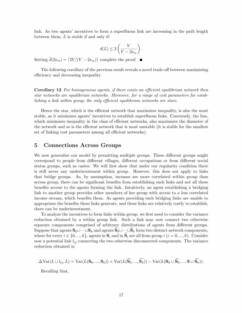
We now generalize our model by permitting multiple groups. These different groups mightcorrespond to people from different villages, different occupations or from different socialstatus groups, such as castes. We will first show that under our regularity condition thereis still never any underinvestment within group. However, this does not apply to linksthat bridge groups. As, by assumption, incomes are more correlated within group thanacross group, there can be significant benefits from establishing such links and not all thesebenefits accrue to the agents forming the link. Intuitively, an agent establishing a bridginglink to another group provides other members of her group with access to a less correlatedincome stream, which benefits them. As agents providing such bridging links are unable toappropriate the benefits these links generate, and these links are relatively costly to establish,there can be underinvestment.

To analyze the incentives to form links within group, we first need to consider the variancereduction obtained by a within group link. Such a link may now connect two otherwiseseparate components comprised of arbitrary distributions of agents from different groups.Suppose that agents S0∪· · ·∪Sk and agents S0∪· · ·∪Sk form two distinct network components,where for every i ∈ 0, ..., k, agents in Si and in Si are all from group i (i = 0, ..., k). Considernow a potential link lij connecting the two otherwise disconnected components. The variancereduction obtained is:

∆ Var(L ∪ lij , L) = Var(L(S0, ...,Sk)) + Var(L(S0, ..., Sk))−Var(L(S0 ∪ S0, ...,S ∪ Sk)).

Recalling that,

17

Var(L(S0,S1, ...,Sk)) =

k∑i=0

(si + si(si − 1)ρw) + 2ρak−1∑i=0

(sik∑

j=i+1sj)

k∑i=0

si

σ2,

some algebra yields26

∆ Var(L ∪ lij , L) =

(1− ρw) +

∑ki=0

(si∑k

j=0 sj − si∑k

j=0 sj

)2(∑ki=0 si

)(∑ki=0 si

)(∑ki=0 si + si

)(ρw − ρa)

σ2. (2)

The key feature of this equation is that it is always weakly greater than (1−ρw)σ2, whichis the variance reduction we found in the previous section when all agents were from the samegroup. So, the presence of across group links within a group only increases the incentives forwithin group links to be formed. This implies that there will still be no under-investmentas long as our regularity condition is met and 2κw ≤ V = λ

2 (1 − ρw)σ2. Recall that thisregularity condition just requires that it is efficient for two agents, both without any otherconnections and in the same group to engage in risk-sharing.

Proposition 13 Under the regularity condition that 2κw ≤ V , there will no under-investmentbetween any two agents from the same group in any stable network.

Motivated by Proposition 13, within group we will continue to focus on the problem ofoverinvestment rather than underinvestment. However, in contrast to Proposition 13, therecan be underinvestment across group. The key insight is that, as opposed to the case ofhomogenous agents, where the value of an essential link does not depend on the sizes of thecomponents it connects, the value of an essential link connecting two different groups of agentsincreases in the sizes of the components. To show this formally, consider an isolated groupthat has no across group connections and consider the incentives for a first such connectionto be formed. Let the first component consists of agents from a single group, say group 0,and the second component consists of agents from any other groups (1 to k). The variancereduction obtained by connected these two components then simplifies to:

∆ Var(L ∪ lij , L) =

(1− ρw) +

s0

((∑ki=1 si

)2+∑k

i=1 s2i

)(∑k

i=1 si

)(s0 +

∑ki=1 si

) (ρw − ρa)

σ2, (3)

∂∆ Var(L ∪ lij , L)

∂s0=

(∑ki=1 si

)2+∑k

i=1 s2i(

s0 +∑k

i=1 si

)2 (ρw − ρa)σ2 > 0. (4)

The inequality follows since ρw > ρa.An immediate implication is that agents i and j, who connect two otherwise unconnected

groups receive a strictly smaller combined private benefit than the social value of the link.

26One of the key steps to simplifying the expression is noting that: 2k−1∑i=0

(sik∑

j=i+1

sj) =

(k∑

i=0

si

)2

−k∑

i=0

s2i .

18

To see why, consider the Myerson Value calculation. In most orders of arrivals when thesecond agent of the pair ij arrives, not all other agents on the components of i and j havearrived yet. Hence, for most orders of arrivals the incremental contribution of the link to theMyerson values of the connecting agents is smaller than the social value of the link. For theremaining orders of arrival the incremental contribution of the link the Myerson value is itssocial value. Averaging over these orders of arrivals, the link contributes less to the Myersonvalues of i and j than its social value leading to the possibility of underinvestment.

We formalize the resulting possibility of underinvestment in Proposition 14.Let Sg = i : G(i) = g denote the agents in group g.

Proposition 14 If m ≥ 2 then underinvestment is possible in equilibrium.

Proof. We will show that if there are m ≥ 2 equal sized groups then there is a range ofparameters κw > 0 and κa > κw such that in any equilibrium all groups are disconnected,despite an extra link connecting any two groups having a strictly positive social value. Byassumption the within group correlation coefficient ρw < 1 and the coefficient of absolute riskaversion λ > 0. Together, these parameter restrictions imply that the certainty equivalentvalue of a variance reduction from connecting one agent to any group of other agents isstrictly positive. So, for κw sufficiently close to 0, in all equilibria any two agents from thesame group must be path connected.

Assume now that all groups form separate network components, and consider a potentialextra link lij connecting groups g and g′. As shown above, the change in total variance, and sosurplus, achieved by connecting agents in Sg to agents in Sg′ is increasing in the size of bothgroups, sg and sg′ respectively. This means that the marginal contribution to total surplus ofthe link lij is higher than the contribution to total surplus when the later of i and j are addedto the network, unless i or j is added last. This implies than MV (i;L ∪ lij) −MV (i;L) <TS(L ∪ lij) − TS(L) for all i ∈ Sg and MV (j;L ∪ lij) −MV (j;L) < TS(L ∪ lij) − TS(L)for all j ∈ Sg′ . There thus exists a range of κa for which MV (i;L ∪ lij) −MV (i;L) < κaand MV (j;L ∪ lij)−MV (j;L) < κa, but TS(L ∪ lij)− TS(L) > 2κa. For such parameters,there is an equilibrium in which within groups agents are completely connected, but there isno link across groups, despite it being socially desirable.

Besides underinvestment, overinvestment is also possible across group. Forming super-fluous links will increase an agent’s share of surplus without improving overall risk sharingand can therefore create incentives to overinvest. Nevertheless, when κa is relatively high,underinvestment rather than overinvestment in across group links will be the main efficiencyconcern. In many settings within group links are relatively cheap to establish in comparisonto across group links. For example, when the different groups correspond to different castes,as in our data, it can be quite costly to be seen to interact with members of the other caste(e.g., Srinivas (1962), Banerjee et al. (2013b)). Motivated by this, and because across grouplinks are considerably sparser in our data (to be described in the next section) than withingroup links, we focus our attention on this parameter region. More concretely, below weinvestigate what within-group network structures create the best incentives to form acrossgroup links and what network structures minimize the incentives for overinvestment withingroup. Remarkably, we will find that these two forces push local network structures in thesame direction, and in both cases towards inequality in the society.

We begin by considering local overinvestment within groups, which corresponds to theforming of superflous within group links. We found in the previous section that, for homoge-

19

nous agents, the star was the efficient network that minimized the incentives for overinvest-ment. However, once we include links to other groups the analysis is more complicated. Thevariance reduction a within group link generates is still zero if the link is superfluous, butwhen the link is essential it now depends on the distribution of agents across the differentgroups the link grants access to. Moreover, the variance reduction may be decreasing orincreasing in the number of people is a specific such group.27 This makes Myerson valuecalculation substantially more complicated. With homogenous agents, all that mattered waswhether the link was essential when added. Now, for each arrival order in which the link isessential, we also need to keep track of the distribution of agents across the different groupswho are being connected. Nevertheless, our earlier result generalizes to this setting, althoughthe argument establishing the result is more subtle.

Proposition 15 The local network structure that minimizes the incentives to overinvestwithin group is the local star, with the center agent holding all across group links. If anyother local network is robust to within group overinvestment, this network is also robust towithin group overinvestment.

Proof. Equation 2 shows that a lower bound on the variance reduction obtained by anessential link connecting any two components is (1 − ρw)σ2. This is the variance reductionobtained by an essential within group link on an isolated component. So, by the Myersoncalculation, starting from an isolated component, adding any set of across group links weaklyincreases the incentives for agents to form superfluous within group links. In other words, wehave found a lower bound on the incentives to overinvest within group.

We now show that the local star, with all across group links held by the center node,achieves this lower bound. The key insight is that the presence of the across group link doesnot increase the incentives for overinvestment within group. Consider two periphery nodesi, j in the same local star, and consider their incentives to form the superfluous link lij . TheMyerson value calculation implies that the agents forming this link receive the link’s averagemarginal contribution to total surplus across all permutations in which the agents can beadded. A necessary condition for the additional link lij to be essential when i is added isthat the central node has not yet been added. Otherwise, there is already a path from i toj (or j has not yet been added). Thus, for every possible permutation, the additional linklij increases i’s average marginal contribution to total surplus by exactly the same amount,regardless of whether the central agent has an across group link or not.

As by Corollary 12 the local star minimized overinvestment incentives absent the across-group link, and as incentives can only be increased by the addition of across group links, thelocal star (with all across group link held by the center agent) must minimize overinvestmentincentives in the presence of across-group links. In other words, once the across-group linksare added (to the center node), the incentives to overinvest within group are no higher forthis network, but are weakly higher for all other efficient networks.

We now consider the local network structures that maximize the incentives for an acrossgroup link to be established. We have already established that the marginal contributionto total surplus of a first bridging link is increasing in the size of the groups it connects. Itfollows that the agents with the strongest incentives to form such links, are those who will

27In the case of an essential across-group link that bridges two otherwise disconnected groups, the com-parative statics are unambiguous. In this case, the variance reduction is increasing in the size of the groupsconnected, as shown by inequality (4).

20

be linked to most other agents within their group when they added to the network in theMyerson calculation. The result below formalizes this intuition.

Let P(Sk) be the set of possible permutations for agents Sk. For any permutation P ∈P(S), let Ti(P ) be the set of agents i is path connected to on L(S′) where S′ is the set

of agents including i drawn weakly before i. Let T(m)i be a random variable equal to the

cardinality of Ti(P ), conditional on i being the m-th agent to be drawn according to P .

We will say that agent i ∈ Sk is more central within group than agent j ∈ Sk, if T(m)i first-

order stochastically dominates T(m)j for all m ∈ 1, 2, ..., |Sk|. In other words, considering

all the permutations in which i is the m-th agent, and all the permutations in which j is them-th agent, the size of i’s component at i’s arrival is larger than that of j’s at j’s arrival inthe sense of first-order stochastic dominance.28 This measure of centrality provides a partialordering of agents.

Proposition 16 Suppose agents in S0 form a network component, and all other agents inN form another network component. Let i, i′ ∈ S0 and let j 6∈ S0. If i is more central withingroup than i′, then i receives a higher payoff from forming lij than i′ receives from formingli′j:

MV (i;L ∪ lij)−MV (i;L) > MV (i′;L ∪ li′j)−MV (i′;L)

Proof. See Appendix A.

The proof of Proposition 16 pairs arrival orders for a more central and less central agentsso that in each case the more central agent, when added, is connected to weakly more peoplein the same group and the same set of people from other groups as the less central agent.Such a pairing of arrival orders is possible from the definition of centrality, and in particularthe first order stochastic dominance it requires.

Proposition 16 shows that more central agents have better incentives to form intergrouplinks. We can then consider the problem of maximizing the incentives to form intergrouplinks by choosing the local network structures (networks containing only within group links).We will say that the local network structures that achieve these maximum possible incentivesare most robust to underinvestment inefficiency across group.

Corollary 17 The efficient local network structure most robust to underinvestment ineffi-ciency across group is the star, with the potential across-group link holder at the center. Ifany other local network is robust to underinvestment across group, then so is the star.

Proof. Within a local network, an agent connected to all other agents is weakly more centralthan any other agent. For any permutation, such an agent is always connected to all otheragents that are before him in the permutation. As no agent can ever be connected to anagent after them in a permutation upon being added to the graph, an agent connected toeveryone else is more central than all other agents and so by Proposition 16 has strongerincentives to form an across group link.

Efficient networks are always trees and the star network is the unique tree network inwhich one agent is directly connected to all others.

28An alternative and equivalent definition is that i is more central than j if there exists a bijectionB : P(Sk) → P(Sk) such that |Ti(P )| ≥ |Tj(B(P ))| and P (i) = P ′(j), where P (i) is i’s position in thepermutation P and P ′ = B(P ).

21

3 11

1

5

13 16

15 14 9

7

12

2

10

8

4

6

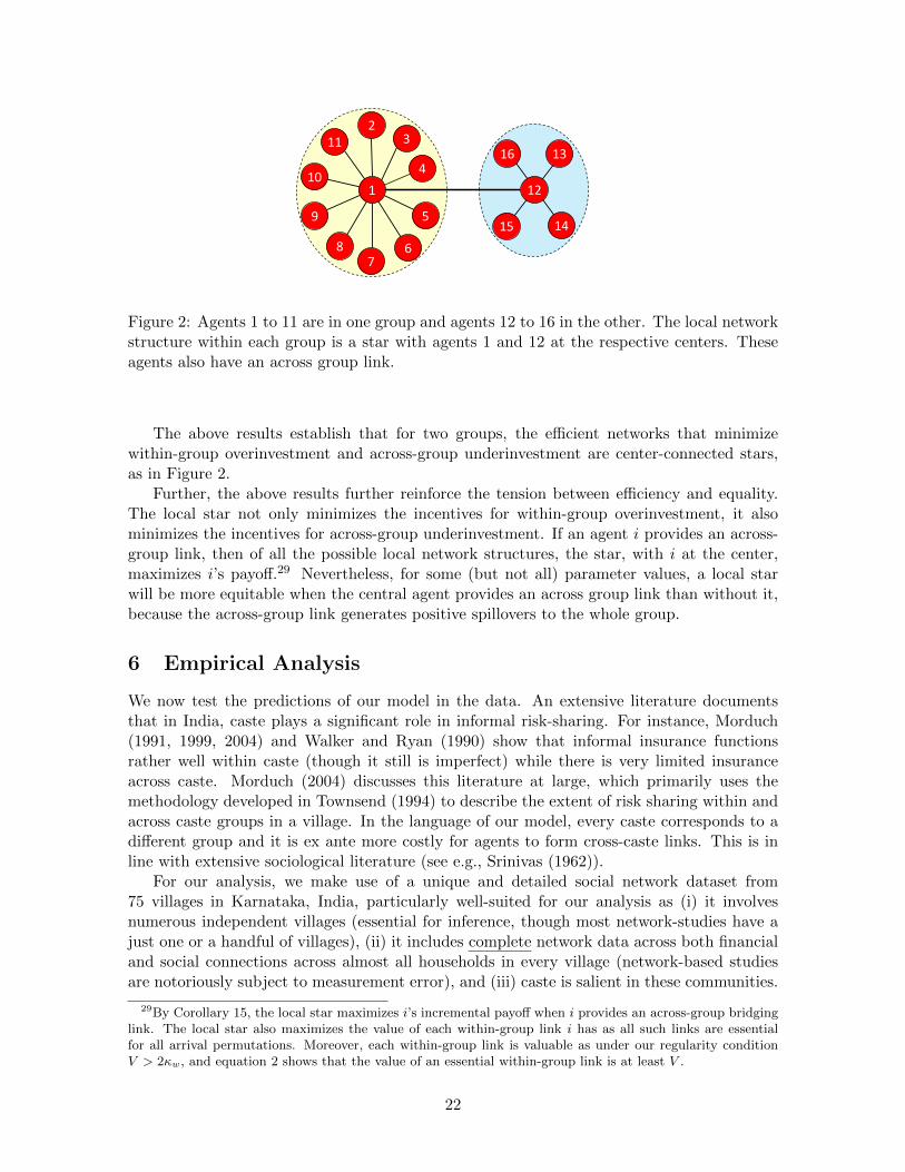
Figure 2: Agents 1 to 11 are in one group and agents 12 to 16 in the other. The local networkstructure within each group is a star with agents 1 and 12 at the respective centers. Theseagents also have an across group link.

The above results establish that for two groups, the efficient networks that minimizewithin-group overinvestment and across-group underinvestment are center-connected stars,as in Figure 2.

Further, the above results further reinforce the tension between efficiency and equality.The local star not only minimizes the incentives for within-group overinvestment, it alsominimizes the incentives for across-group underinvestment. If an agent i provides an across-group link, then of all the possible local network structures, the star, with i at the center,maximizes i’s payoff.29 Nevertheless, for some (but not all) parameter values, a local starwill be more equitable when the central agent provides an across group link than without it,because the across-group link generates positive spillovers to the whole group.

6 Empirical Analysis

We now test the predictions of our model in the data. An extensive literature documentsthat in India, caste plays a significant role in informal risk-sharing. For instance, Morduch(1991, 1999, 2004) and Walker and Ryan (1990) show that informal insurance functionsrather well within caste (though it still is imperfect) while there is very limited insuranceacross caste. Morduch (2004) discusses this literature at large, which primarily uses themethodology developed in Townsend (1994) to describe the extent of risk sharing within andacross caste groups in a village. In the language of our model, every caste corresponds to adifferent group and it is ex ante more costly for agents to form cross-caste links. This is inline with extensive sociological literature (see e.g., Srinivas (1962)).

For our analysis, we make use of a unique and detailed social network dataset from75 villages in Karnataka, India, particularly well-suited for our analysis as (i) it involvesnumerous independent villages (essential for inference, though most network-studies have ajust one or a handful of villages), (ii) it includes complete network data across both financialand social connections across almost all households in every village (network-based studiesare notoriously subject to measurement error), and (iii) caste is salient in these communities.

29By Corollary 15, the local star maximizes i’s incremental payoff when i provides an across-group bridginglink. The local star also maximizes the value of each within-group link i has as all such links are essentialfor all arrival permutations. Moreover, each within-group link is valuable as under our regularity conditionV > 2κw, and equation 2 shows that the value of an essential within-group link is at least V .

22

6.1 Setting and Data

The data we use were collected by Banerjee, Chandrasekhar, Duflo and Jackson (2013, 2014)from 75 villages in Karnataka, India. In 2011, the authors conducted a survey in the 75villages. The villages span 5 districts and range 2-3 hour drive outside of Bangalore. Theyare far enough apart to be treated as independent systems (the median distance is 46km anda district has between 1000-3000 villages). The survey included a village questionnaire, acensus of all households, demographic covariates (including caste and occupation), as well asdata on a number of amenities (e.g., roofing, latrine or electricity access quality). A detailedindividual level survey was administered to most adults in every village. The survey includeda networks module with twelve dimensions of relationships including financial relationships,social relationships, and advice relationships.30

Our analysis focuses on two types of networks: the financial graph, LF , and the socialgraph, LS . The financial graphs represent risk-sharing connections and the social graphrepresents friendships/links used to socialize. We build “AND” networks, which say a linkexists if it exists on every dimension being considered (various types of financial connectionson the financial network, and various types of social connections on the social network).31

The advantage of doing this is that it generates a network structure that is more robustto independent measurement error. 32 In some of our empirical analysis, we will explicitlyconsider how our predictions differentially play out in LF relative to LS , as our theory speaksto the former.

As our theory pertains to networks formed from multiple groups, here we make use ofcaste. Motivated by the social structure of our communities, and following Munshi (2006)and Banerjee et al. (2013), we partition our individuals into two caste groups: scheduledcaste/scheduled tribes (SC/ST) and general merit/otherwise backward castes (GM/OBC).These are governmental designations used to condition the allocation of, for instance, schoolseating by caste and reflect a core fissure in the social fabric.Table 1 provides some summary statistics for our data. The average number of householdsper village is 209 with a standard deviation of 80. The average degree of the financial graphis 3.1 and the social graph is 1.7. It is interesting to note that the financial graph is moredense. Further, we see that the clustering in the financial graph is 0.18 (0.06) whereas for thesocial graph it is 0.05 (0.03). Though the density is only 1.8 times higher for the financialgraph than the social graph, the fact that the clustering is over 3 times higher for the financialgraph is of note. This is consistent with the results of, for instance, Jackson et al. (2012)that financial links may need to be supported/embedded in cliques to sustain cooperation.Both the financial and social networks exhibit relatively few cross-caste links. This is seenlooking at the ratio of the probability of having a cross-caste link relative to the probabilityof having a within-caste link. A within-caste link is five times more likely in the financialgraph and three times more likely in the social graph. Finally, 67% of households are highcaste (GM or OBC). We describe our main outcome variables later.

30See Banerjee et al. (2014) for more details. In total we have network data from 89.14% of the 16,476households based on interviews with 65% of all adult individuals aged 18-55.

31We say lij ∈ LF if i goes to j to borrow money in times of need, j goes to i to borrow money in timesof need, i goes to j to borrow material goods such as kerosene, rice or oil in times of need, and j goes to i toborrow material goods in times of need.

32We say lij ∈ LS if i goes to j’s house to socialize, j goes to i’s house to socialize, i goes to j for advice,and j goes to i for advice.

23

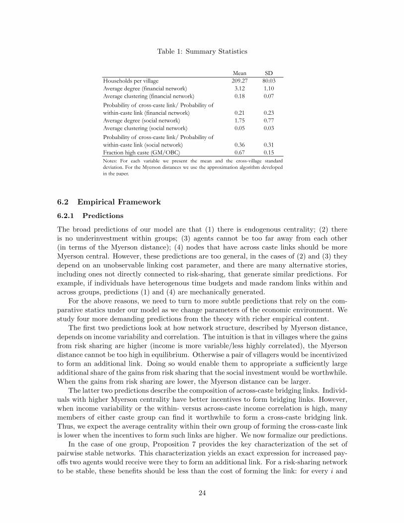
Table 1: Summary Statistics

Mean SDHouseholds per village 209.27 80.03Average degree (financial network) 3.12 1.10Average clustering (financial network) 0.18 0.07Probability of cross-caste link/ Probability of within-caste link (financial network) 0.21 0.23Average degree (social network) 1.75 0.77Average clustering (social network) 0.05 0.03Probability of cross-caste link/ Probability of within-caste link (social network) 0.36 0.31Fraction high caste (GM/OBC) 0.67 0.15Notes: For each variable we present the mean and the cross-village standarddeviation. For the Myerson distances we use the approximation algorithm developedin the paper.

6.2 Empirical Framework

6.2.1 Predictions

The broad predictions of our model are that (1) there is endogenous centrality; (2) thereis no underinvestment within groups; (3) agents cannot be too far away from each other(in terms of the Myerson distance); (4) nodes that have across caste links should be moreMyerson central. However, these predictions are too general, in the cases of (2) and (3) theydepend on an unobservable linking cost parameter, and there are many alternative stories,including ones not directly connected to risk-sharing, that generate similar predictions. Forexample, if individuals have heterogenous time budgets and made random links within andacross groups, predictions (1) and (4) are mechanically generated.

For the above reasons, we need to turn to more subtle predictions that rely on the com-parative statics under our model as we change parameters of the economic environment. Westudy four more demanding predictions from the theory with richer empirical content.

The first two predictions look at how network structure, described by Myerson distance,depends on income variability and correlation. The intuition is that in villages where the gainsfrom risk sharing are higher (income is more variable/less highly correlated), the Myersondistance cannot be too high in equilibrium. Otherwise a pair of villagers would be incentivizedto form an additional link. Doing so would enable them to appropriate a sufficiently largeadditional share of the gains from risk sharing that the social investment would be worthwhile.When the gains from risk sharing are lower, the Myerson distance can be larger.

The latter two predictions describe the composition of across-caste bridging links. Individ-uals with higher Myerson centrality have better incentives to form bridging links. However,when income variability or the within- versus across-caste income correlation is high, manymembers of either caste group can find it worthwhile to form a cross-caste bridging link.Thus, we expect the average centrality within their own group of forming the cross-caste linkis lower when the incentives to form such links are higher. We now formalize our predictions.

In the case of one group, Proposition 7 provides the key characterization of the set ofpairwise stable networks. This characterization yields an exact expression for increased pay-offs two agents would receive were they to form an additional link. For a risk-sharing networkto be stable, these benefits should be less than the cost of forming the link: for every i and

24

j that do not have a link,

md(i, j, L) ≤ 2κw(1− ρw)λσ2

. (5)

In our empirical setting, we are interested in Indian village networks where there are multiplegroups, given by caste. Nevertheless, the inequality in (5) provides an appropriate benchmarkfor within-group links. Recall that the left side of the inequality captures the probability thatthe link is not essential for a random permutation in the arrival order and the right side givesthe value of the variance reduction obtained. The key complication is that when a within-group link is essential for a subgraph, but it connects two otherwise separate components thatcontain people from multiple groups, then the value of the variance reduction will depend onthe composition of people within the two components.

Consider the variance reduction obtained by combining any two components, with agentsS0, . . . ,Sk and S0, . . . , Sk respectively. From equation 2, this certainty equivalent value ofthis variance reduction is:

[(1− ρw) + f(s0, . . . , sk, s0, . . . , sk)(ρw − ρa)]λσ2

2.

This term is hard to compute in general. Here we approximate it by assuming that thedistribution of people from each group is the same within each component, so si = α andsi = β for i = 0, . . . , k.

Proposition 18 The certainty equivalent value of variance reduction obtained by linking acomponent with α people from each of groups 0, ..., k to a component with β people from eachof groups 0, ..., k is:

(1− ρw)λσ2

2.

Proof. See the Appendix A.

Proposition 18 shows that the variance reduction obtained by permitting two componentscontaining agents from multiple groups to risk share is the same as when all agents arefrom the same group, as long the proportion of people from each group is the same in eachcomponent.

The above considerations lead to the following predictions:

P1. In villages with higher σ2, the average Myerson distance should be smaller.

P2. In villages with lower ρw, the average Myerson distance should be smaller.

While our first set of predictions looks at the relationship between the Myerson distanceand the environmental parameters, our second set of predictions looks at the composition ofthe links. Our interest is in which agents provide the across group links. Proposition 16 showsmore central agents have better incentives to provide an across-group link. The importanceof centrality will depend on the overall strength of the incentives to form across-caste links.When income variance is high, or within-caste income correlation is high relative to across-caste income correlation, the incentives to form an across-caste link will also be high and sonetwork position will be less important; villagers in more varied locations will have sufficientincentives to form across-caste links. More formally, from the variance reduction given inequation 2 it is straightforward to show that for an across-caste bridging link lij :

25

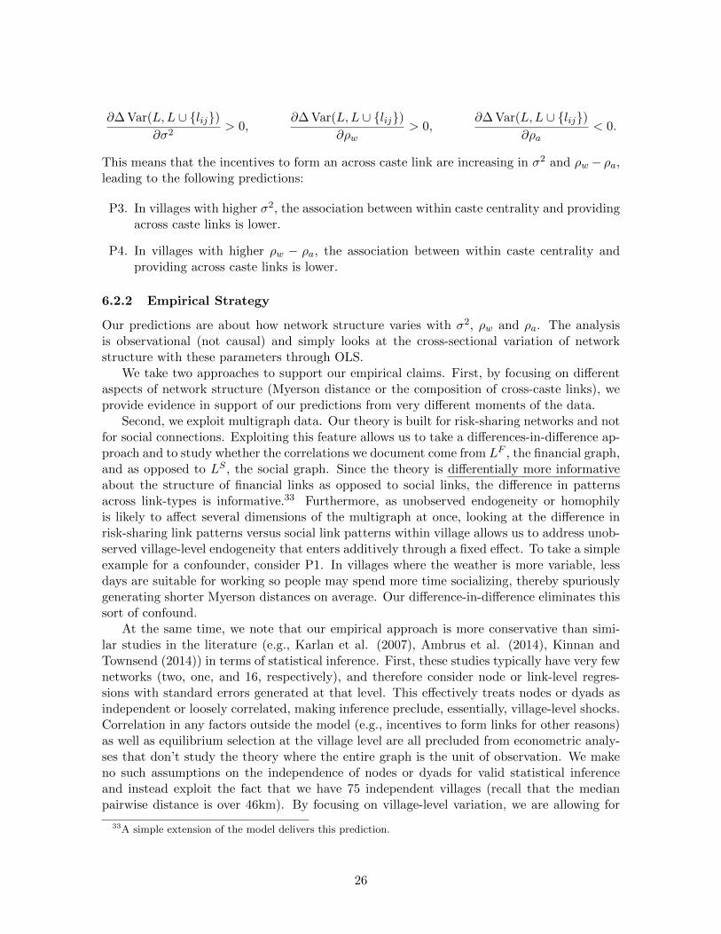
∂∆ Var(L,L ∪ lij)∂σ2

> 0,∂∆ Var(L,L ∪ lij)

∂ρw> 0,

∂∆ Var(L,L ∪ lij)∂ρa

< 0.

This means that the incentives to form an across caste link are increasing in σ2 and ρw − ρa,leading to the following predictions:

P3. In villages with higher σ2, the association between within caste centrality and providingacross caste links is lower.

P4. In villages with higher ρw − ρa, the association between within caste centrality andproviding across caste links is lower.

6.2.2 Empirical Strategy

Our predictions are about how network structure varies with σ2, ρw and ρa. The analysisis observational (not causal) and simply looks at the cross-sectional variation of networkstructure with these parameters through OLS.

We take two approaches to support our empirical claims. First, by focusing on differentaspects of network structure (Myerson distance or the composition of cross-caste links), weprovide evidence in support of our predictions from very different moments of the data.

Second, we exploit multigraph data. Our theory is built for risk-sharing networks and notfor social connections. Exploiting this feature allows us to take a differences-in-difference ap-proach and to study whether the correlations we document come from LF , the financial graph,and as opposed to LS , the social graph. Since the theory is differentially more informativeabout the structure of financial links as opposed to social links, the difference in patternsacross link-types is informative.33 Furthermore, as unobserved endogeneity or homophilyis likely to affect several dimensions of the multigraph at once, looking at the difference inrisk-sharing link patterns versus social link patterns within village allows us to address unob-served village-level endogeneity that enters additively through a fixed effect. To take a simpleexample for a confounder, consider P1. In villages where the weather is more variable, lessdays are suitable for working so people may spend more time socializing, thereby spuriouslygenerating shorter Myerson distances on average. Our difference-in-difference eliminates thissort of confound.

At the same time, we note that our empirical approach is more conservative than simi-lar studies in the literature (e.g., Karlan et al. (2007), Ambrus et al. (2014), Kinnan andTownsend (2014)) in terms of statistical inference. First, these studies typically have very fewnetworks (two, one, and 16, respectively), and therefore consider node or link-level regres-sions with standard errors generated at that level. This effectively treats nodes or dyads asindependent or loosely correlated, making inference preclude, essentially, village-level shocks.Correlation in any factors outside the model (e.g., incentives to form links for other reasons)as well as equilibrium selection at the village level are all precluded from econometric analy-ses that don’t study the theory where the entire graph is the unit of observation. We makeno such assumptions on the independence of nodes or dyads for valid statistical inferenceand instead exploit the fact that we have 75 independent villages (recall that the medianpairwise distance is over 46km). By focusing on village-level variation, we are allowing for

33A simple extension of the model delivers this prediction.

26

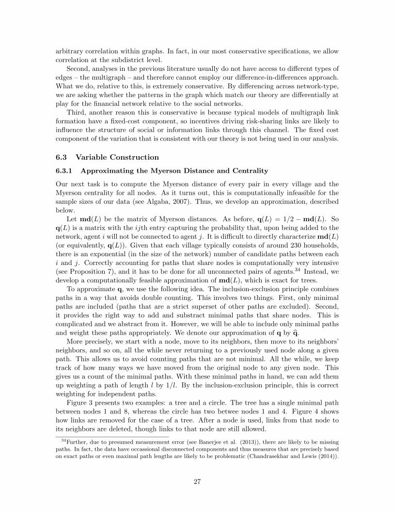
arbitrary correlation within graphs. In fact, in our most conservative specifications, we allowcorrelation at the subdistrict level.

Second, analyses in the previous literature usually do not have access to different types ofedges – the multigraph – and therefore cannot employ our difference-in-differences approach.What we do, relative to this, is extremely conservative. By differencing across network-type,we are asking whether the patterns in the graph which match our theory are differentially atplay for the financial network relative to the social networks.

Third, another reason this is conservative is because typical models of multigraph linkformation have a fixed-cost component, so incentives driving risk-sharing links are likely toinfluence the structure of social or information links through this channel. The fixed costcomponent of the variation that is consistent with our theory is not being used in our analysis.

6.3 Variable Construction

6.3.1 Approximating the Myerson Distance and Centrality

Our next task is to compute the Myerson distance of every pair in every village and theMyerson centrality for all nodes. As it turns out, this is computationally infeasible for thesample sizes of our data (see Algaba, 2007). Thus, we develop an approximation, describedbelow.

Let md(L) be the matrix of Myerson distances. As before, q(L) = 1/2 −md(L). Soq(L) is a matrix with the ijth entry capturing the probability that, upon being added to thenetwork, agent i will not be connected to agent j. It is difficult to directly characterize md(L)(or equivalently, q(L)). Given that each village typically consists of around 230 households,there is an exponential (in the size of the network) number of candidate paths between eachi and j. Correctly accounting for paths that share nodes is computationally very intensive(see Proposition 7), and it has to be done for all unconnected pairs of agents.34 Instead, wedevelop a computationally feasible approximation of md(L), which is exact for trees.

To approximate q, we use the following idea. The inclusion-exclusion principle combinespaths in a way that avoids double counting. This involves two things. First, only minimalpaths are included (paths that are a strict superset of other paths are excluded). Second,it provides the right way to add and substract minimal paths that share nodes. This iscomplicated and we abstract from it. However, we will be able to include only minimal pathsand weight these paths appropriately. We denote our approximation of q by q.

More precisely, we start with a node, move to its neighbors, then move to its neighbors’neighbors, and so on, all the while never returning to a previously used node along a givenpath. This allows us to avoid counting paths that are not minimal. All the while, we keeptrack of how many ways we have moved from the original node to any given node. Thisgives us a count of the minimal paths. With these minimal paths in hand, we can add themup weighting a path of length l by 1/l. By the inclusion-exclusion principle, this is correctweighting for independent paths.

Figure 3 presents two examples: a tree and a circle. The tree has a single minimal pathbetween nodes 1 and 8, whereas the circle has two betwee nodes 1 and 4. Figure 4 showshow links are removed for the case of a tree. After a node is used, links from that node toits neighbors are deleted, though links to that node are still allowed.

34Further, due to presumed measurement error (see Banerjee et al. (2013)), there are likely to be missingpaths. In fact, the data have occassional disconnected components and thus measures that are precisely basedon exact paths or even maximal path lengths are likely to be problematic (Chandrasekhar and Lewis (2014)).

27

1

2 3

4 5 6 7

8 9 10

11

(a) Tree

2

4 5

6 3

7

1

(b) Circle

Figure 3: The i,j – when we are computing md(i, j, L) – are given in purple. The tree containsa single minimal path (orange) whereas the circle contains two (orange and blue).

A

B

(a)

A

B

(b)

A

B

(c)

A

B

(d)

Figure 4: As the algorithm progresses directed links to nodes that have already been reachedare deleted. This makes sure only minimal paths are included. In this case, as in all treenetworks, there is a unique minimal path from A to B.

To build intuition and show our algorithm’s limitations, consider a circle with 7 nodes.We want to compute md(1, 4) as in Figure 3. We need to compute the quantity for eachminimal path, but by the inclusion-exclusion principle, need to subtract the event that bothare present. The long path contributes 1/5 (1 added last in 1,7,6,5,4), the short path 1/4,and by the inclusion-exclusion principle we subtract 1/7 (1 added last in 1,2,...,6,7). Thuswe see

q(1, 4) =1

5+

1

4− 1

7and q(1, 4) =

1

5+

1

4.

Algorithm 19 (Approximation of q) Let ei be the ith basis vector. Initialize q = zeros(n, n),a matrix of zeros. Initialize zt,i = zeros(n, 1) and xt,i = zeros(n, 1) to be n-vectors of zeros,indexed by i = 1, ..., n and t = 1, ..., T . Repeat steps (1-4) for all (e1, ..., en) to compute q.

1. Period 1: There is no identification nor updating steps.

(a) Percolation: x1,i = Aei.

2. Period 2, given (x1,i,A):

28

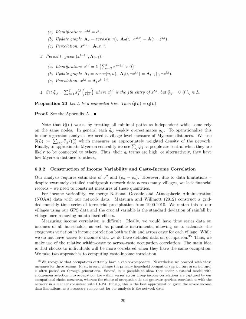
(a) Identification: z2,i = ei.

(b) Update graph: A2 = zeros(n, n), A2(:,¬z2,i) = A(:,¬z2,i).

(c) Percolation: x2,i = A2x1,i.

3. Period t, given (xt−1,i,At−1):

(a) Identification: zt,i = 1∑t

s=2 xs−2,i > 0

.

(b) Update graph: At = zeros(n, n), At(:,¬zt,i) = At−1(:,¬zt,i).(c) Percolation: xt,i = Atx

t−1,i.

4. Set qij =∑T

t=1 xt,ij

(1t+1

)where xt,ij is the jth entry of xt,i, but qij = 0 if lij ∈ L.

Proposition 20 Let L be a connected tree. Then q(L) = q(L).

Proof. See the Appendix A.

Note that q(L) works by treating all minimal paths as independent while some relyon the same nodes. In general each qij weakly overestimates qij . To operationalize thisin our regression analysis, we need a village level measure of Myerson distances. We useq(L) :=

∑i<j qij/

(n2

)which measures an appropriately weighted density of the network.

Finally, to approximate Myerson centrality we use∑

j qij as people are central when they arelikely to be connected to others. Thus, their qi terms are high, or alternatively, they havelow Myerson distance to others.

6.3.2 Construction of Income Variability and Caste-Income Correlation

Our analysis requires estimates of σ2 and (ρw − ρa). However, due to data limitations –despite extremely detailed multigraph network data across many villages, we lack financialrecords – we need to construct measures of these quantities.

For income variability, we merge National Oceanic and Atmospheric Administration(NOAA) data with our network data. Matsuura and Willmott (2012) construct a grid-ded monthly time series of terrestrial precipitation from 1900-2010. We match this to ourvillages using our GPS data and the crucial variable is the standard deviation of rainfall byvillage once removing month fixed-effects.

Measuring income correlation is difficult. Ideally, we would have time series data onincomes of all households, as well as plausible instruments, allowing us to calculate theexogenous variation in income correlation both within and across caste for each village. Whilewe do not have access to income data, we do have detailed data on occupation.35 Thus, wemake use of the relative within-caste to across-caste occupation correlation. The main ideais that shocks to individuals will be more correlated when they have the same occupation.We take two approaches to computing caste-income correlation.

35We recognize that occupations certainly have a choice-component. Nevertheless we proceed with thesemeasures for three reasons. First, in rural villages the primary household occupation (agriculture or sericulture)is often passed on through generations. Second, it is possible to show that under a natural model withendogenous selection into occupation, the within versus across group income correlations are captured by ouroccupational choice measures, whereas the choice of occupation do not generate spurious correlations with thenetwork in a manner consistent with P1-P4. Finally, this is the best approximation given the severe incomedata limitations, as a necessary component for our analysis is the network data.

29

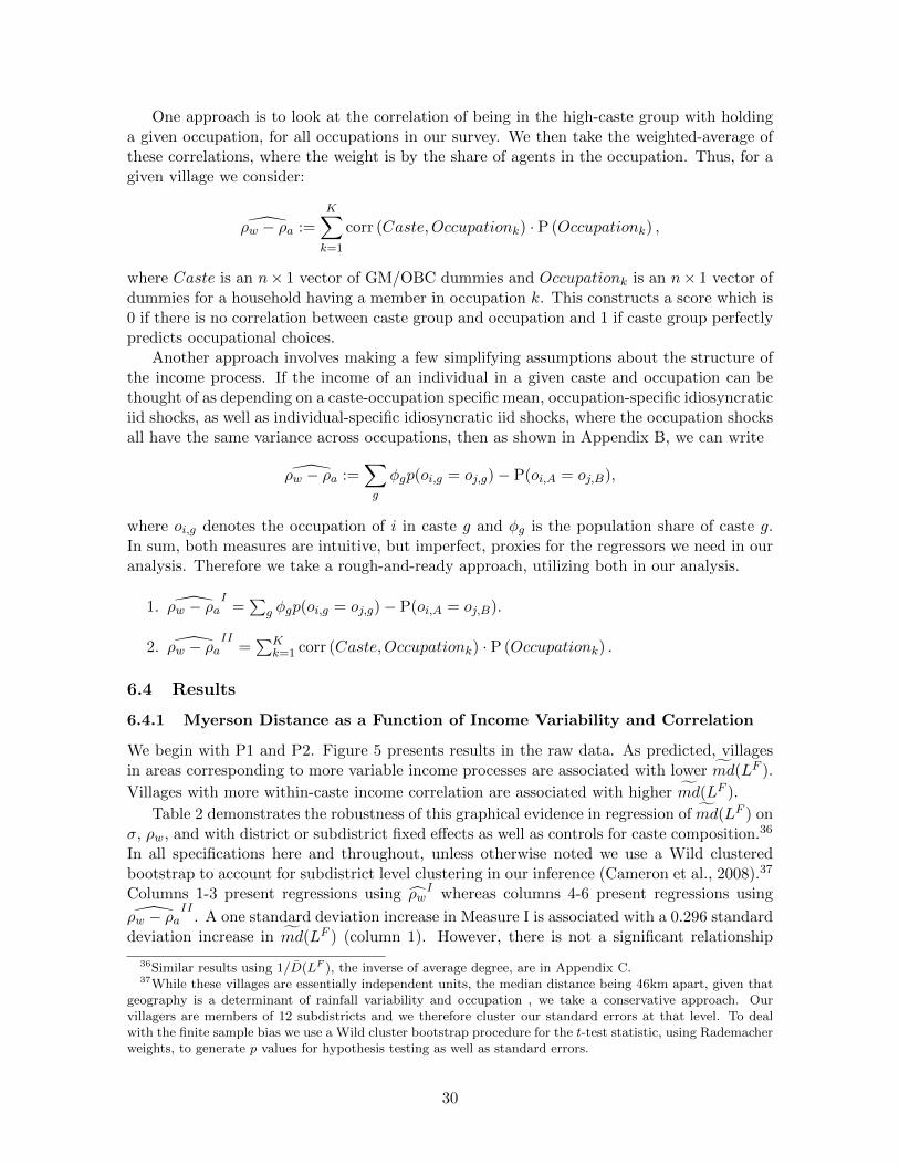
One approach is to look at the correlation of being in the high-caste group with holdinga given occupation, for all occupations in our survey. We then take the weighted-average ofthese correlations, where the weight is by the share of agents in the occupation. Thus, for agiven village we consider:

ρw − ρa :=K∑k=1

corr (Caste,Occupationk) · P (Occupationk) ,

where Caste is an n× 1 vector of GM/OBC dummies and Occupationk is an n× 1 vector ofdummies for a household having a member in occupation k. This constructs a score which is0 if there is no correlation between caste group and occupation and 1 if caste group perfectlypredicts occupational choices.

Another approach involves making a few simplifying assumptions about the structure ofthe income process. If the income of an individual in a given caste and occupation can bethought of as depending on a caste-occupation specific mean, occupation-specific idiosyncraticiid shocks, as well as individual-specific idiosyncratic iid shocks, where the occupation shocksall have the same variance across occupations, then as shown in Appendix B, we can write

ρw − ρa :=∑g

φgp(oi,g = oj,g)− P(oi,A = oj,B),

where oi,g denotes the occupation of i in caste g and φg is the population share of caste g.In sum, both measures are intuitive, but imperfect, proxies for the regressors we need in ouranalysis. Therefore we take a rough-and-ready approach, utilizing both in our analysis.

1. ρw − ρaI

=∑

g φgp(oi,g = oj,g)− P(oi,A = oj,B).

2. ρw − ρaII

=∑K

k=1 corr (Caste,Occupationk) · P (Occupationk) .

6.4 Results

6.4.1 Myerson Distance as a Function of Income Variability and Correlation

We begin with P1 and P2. Figure 5 presents results in the raw data. As predicted, villagesin areas corresponding to more variable income processes are associated with lower md(LF ).

Villages with more within-caste income correlation are associated with higher md(LF ).

Table 2 demonstrates the robustness of this graphical evidence in regression of md(LF ) onσ, ρw, and with district or subdistrict fixed effects as well as controls for caste composition.36

In all specifications here and throughout, unless otherwise noted we use a Wild clusteredbootstrap to account for subdistrict level clustering in our inference (Cameron et al., 2008).37

Columns 1-3 present regressions using ρwI whereas columns 4-6 present regressions using

ρw − ρaII

. A one standard deviation increase in Measure I is associated with a 0.296 standarddeviation increase in md(LF ) (column 1). However, there is not a significant relationship

36Similar results using 1/D(LF ), the inverse of average degree, are in Appendix C.37While these villages are essentially independent units, the median distance being 46km apart, given that

geography is a determinant of rainfall variability and occupation , we take a conservative approach. Ourvillagers are members of 12 subdistricts and we therefore cluster our standard errors at that level. To dealwith the finite sample bias we use a Wild cluster bootstrap procedure for the t-test statistic, using Rademacherweights, to generate p values for hypothesis testing as well as standard errors.

30

(a) Measure: md(LF ) vs σ2 (b) Measure: md(LF ) vs ρw

Figure 5: Myerson distance in standardized units against the variability of rainfall at thevillage level and the within-caste income correlation metric, both in standardized units.

Table 2: Myerson distance vs. income variability and correlation

(1) (2) (3) (4) (5) (6)Income Correlation 0.296 0.109 -0.001 0.205 0.182 0.098

(0.109) (0.061) (0.064) (0.088) (0.069) (0.063)[0.004] [0.12] [0.996] [0.03] [0.012] [0.13]

Income Variability -0.061 0.015 -0.281 -0.054 -0.054 -0.304(0.187) (0.239) (0.094) (0.206) (0.224) 0.101[0.82] [0.928] [0.002] [0.774] [0.794] [0.002]

District FE N Y Y N Y YSubdistrict FE N N Y N N YR-squared 0.1066 0.5701 0.7458 0.071 0.5897 0.7525

Measure I Measure II

Notes: Outcome variable is the average Myerson distance, computed by the approximation algorithm.Outcome variables and regressors scaled by their standard deviations. Columns (1-3) use Measure I of thecaste-income correlation, whereas columns (4-6) use Measure II. Specifications include control for castecomposition: p(1-p), where p is share in high caste. Wild clustered bootstrap standard errors are presentedin (.), using Rademacher weights. The cluster is at the subdistrict level, of which there are 12. 1000 samplesare used per bootstrap. p-values from the Wild clustered bootstrap t are presented in [.].

between income variability and md(LF ) in this specification. Column 4 presents the analogous

results using ρw − ρaII

. Again a one standard deviation in Measure II is associated witha 0.205 standard deviation increase in md(LF ), but income variability has no detectablecorrelation with the outcome variable (column 4). In columns 2 and 5 we add district fixedeffects and the results are mostly reflective of those in columns 1 and 3. A one standarddeviation increase in income correlation corresponds to a 0.11 or 0.18 standard deviationincrease in Myerson distance, using Measure I (p-value 0.12) and Measure II (p-value 0.012)respectively. Finally, when we include subdistrict fixed effects, our estimate under Measure Iis too noisy to distinguish from zero, though we find similar evidence under Measure II (a 0.1standard deviation effect, p-value 0.13). Further, when comparing villages within subdistrictwe are able to identify an income variability effect. A one standard deviation increase inincome variability is associated with a 0.28 or 0.3 standard deviation decrease in the averageMyerson distance (columns 3 and 6, respectively).

Taken together, we show increases in within-caste income correlation is associated with

31

Myerson distance in a manner consistent with our theory though the evidence for incomevariability is considerably weaker.

6.4.2 Differences by network type

Next we use a difference-in-differences approach and see whether the effects we are interestedare coming differentially from the financial graph as opposed to the social graph. Figure 6presents the raw data, differenced, graphically. Villages in areas corresponding to more corre-lated within-caste income processes are associated with greater md(LF )−md(LS). Similarly,an increase in the income variability is associated with a differential decrease in the measureof network density in the financial graph as compared to the social graph.

(a) md(LF )− md(LS) vs σ2 (b) md(LF )− md(LS) vs ρw

Figure 6: Myerson distance, differenced across network type, versus income variability orwithin-caste income correlation.

Let v index village and t ∈ F, S index network type. We use the following regressions:

Yv,t = α+ β · σv · 1t=F + γ · ρw,v · 1t=F + µv + δ ·Xv · 1t=F + εv,t,

where Yv,t = md(Ltv), µv is a possibly endogenous village fixed-effect, and Xv are village-levelcontrols. P1 and P2 correspond to β < 0 and γ > 0, since our theory pertains only to risk-sharing networks. Thus, our effects should be differentially more predictive for the financialnetwork and not the social network and should remain true when looking at relative effects.

Table 3 presents the results. We find that a one standard deviation increase in incomevariability differentially decreases md(L) by about 0.24 standard deviations more in financialnetworks than social networks (columns 1, 4), irrespective of the measure of income correla-tion used. Similarly, a one standard deviation increase in Measure II differentially increasesmd(L) by 0.16 standard deviations more in financial networks than social networks (column2). However, we find no association using Measure I for the income correlation.

Thus, even when we look within-village, by allowing for village fixed effects, and yetallowing for subdistrict level correlation in our error terms, we see that the financial graphbehave in a manner consistent with the theory relative to the social graph.

6.4.3 Association between within-caste centrality and cross-caste links

We now look at how the composition of cross caste links vary with these parameters. P3shows that in villages with higher variability we should see a greater association between

32

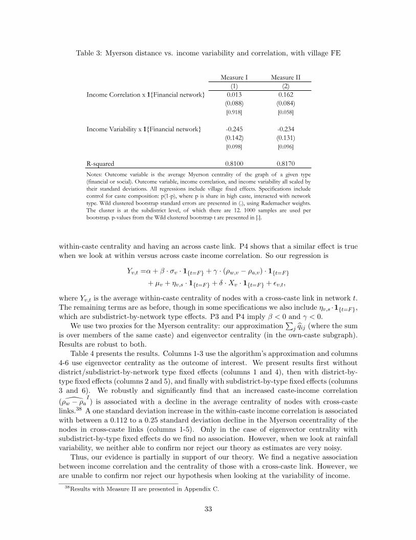
Table 3: Myerson distance vs. income variability and correlation, with village FE

Measure I Measure II(1) (2)

Income Correlation x 1Financial network 0.013 0.162(0.088) (0.084)[0.918] [0.058]

Income Variability x 1Financial network -0.245 -0.234(0.142) (0.131)[0.098] [0.096]

R-squared 0.8100 0.8170

Notes: Outcome variable is the average Myerson centrality of the graph of a given type(financial or social). Outcome variable, income correlation, and income variability all scaled bytheir standard deviations. All regressions include village fixed effects. Specifications includecontrol for caste composition: p(1-p), where p is share in high caste, interacted with networktype. Wild clustered bootstrap standard errors are presented in (.), using Rademacher weights.The cluster is at the subdistrict level, of which there are 12. 1000 samples are used perbootstrap. p-values from the Wild clustered bootstrap t are presented in [.].

within-caste centrality and having an across caste link. P4 shows that a similar effect is truewhen we look at within versus across caste income correlation. So our regression is

Yv,t =α+ β · σv · 1t=F + γ · (ρw,v − ρa,v) · 1t=F+ µv + ηv,s · 1t=F + δ ·Xv · 1t=F + εv,t,

where Yv,t is the average within-caste centrality of nodes with a cross-caste link in network t.The remaining terms are as before, though in some specifications we also include ηv,s ·1t=F,which are subdistrict-by-network type effects. P3 and P4 imply β < 0 and γ < 0.

We use two proxies for the Myerson centrality: our approximation∑

j qij (where the sumis over members of the same caste) and eigenvector centrality (in the own-caste subgraph).Results are robust to both.

Table 4 presents the results. Columns 1-3 use the algorithm’s approximation and columns4-6 use eigenvector centrality as the outcome of interest. We present results first withoutdistrict/subdistrict-by-network type fixed effects (columns 1 and 4), then with district-by-type fixed effects (columns 2 and 5), and finally with subdistrict-by-type fixed effects (columns3 and 6). We robustly and significantly find that an increased caste-income correlation

( ρw − ρaI) is associated with a decline in the average centrality of nodes with cross-caste

links.38 A one standard deviation increase in the within-caste income correlation is associatedwith between a 0.112 to a 0.25 standard deviation decline in the Myerson cecentrality of thenodes in cross-caste links (columns 1-5). Only in the case of eigenvector centrality withsubdistrict-by-type fixed effects do we find no association. However, when we look at rainfallvariability, we neither able to confirm nor reject our theory as estimates are very noisy.

Thus, our evidence is partially in support of our theory. We find a negative associationbetween income correlation and the centrality of those with a cross-caste link. However, weare unable to confirm nor reject our hypothesis when looking at the variability of income.

38Results with Measure II are presented in Appendix C.

33

Table 4: Association between average within-caste centrality of nodes with cross-caste linksand measures of rainfall variability and within-caste income correlation

(1) (2) (3) (4) (5) (6)Income Correlation x 1Financial network -0.222 -0.252 -0.112 -0.148 -0.191 -0.064

(0.064) (0.036) (0.057) (0.060) (0.085) (0.095)[0.002] [0.029] [0.052] [0.012] [0.032] [0.54]

Income Variability x 1Financial network 0.261 -0.313 -0.130 0.075 -0.261 -0.291(0.201) (0.295) (0.172) (0.129) (0.170) (0.172)[0.244] [0.472] [0.502] [0.662] [0.227] [0.121]

District x 1Financial network FE N Y Y Y Y YSubdistrict x 1Financial network FE N N Y N Y YR-squared 0.196 0.529 0.675 0.054 0.137 0.346

Myerson Centrality Eigenvector Centrality

Notes: Outcome variable is the Myerson centrality, computed using our approximation algorithm, or eigenvector centrality. Incomecorrelation given by Measure I. Outcome variables and regressors are scaled by their standard deviations. All specifications use villagefixed effects and caste composition controls. Columns 2 and 4 include district-by-network type fixed effects and columns 3 and 6include subdistrict-by-network type fixed effects. Wild clustered bootstrap standard errors are presented in (.), using Rademacherweights. The cluster is at the subdistrict level, of which there are 12. 1000 samples are used per bootstrap. p-values from the Wildclustered bootstrap t are presented in [.].

6.5 Discussion

This section provided suggestive evidence, consistent with our theory, demonstrating:

1. Networks have higher Myerson distance with more within group income correlation.

2. Networks exhibit lower Myerson distance when there is more variable rainfall.

3. Networks exhibit stronger associations between within-group centrality and across-group linking when within-group income correlation is higher, though we detect norelationship with variability of rainfall.

4. Results (1)-(3) are robust to a difference-in-differences approach. By differencing outthe social graph, we can remove village-fixed endogenous factors and more convincinglyargue that the underlying force concerns risk sharing.

Having several distinct prediction is useful as we are conducting an observational analysis.That all significant correlations are consistent with our theory, and we find no falsification,is encouraging.

Of course, there are several other stories consistent with the income variability prediction.For instance, one may think that any theory where the returns to investing in risk-sharingrelationships go up should predict more dense networks. We note, however, that this predic-tion does not hold in Bramoulle and Kranton (2007a), which is perhaps the closest paper toours. In their model, increased variability has no effect on the equilibrium network structure.

Furthermore, our compositional story is new. More generally, P3-P4 are either specificto the risk sharing relationships between castes or differences in income correlations betweencastes, and so within the literature are unique to our model. These predictions are also moresubtle. For instance, higher within group correlation leading to more sparse risk sharingnetworks is not a conclusion of other risk-sharing network formation stories.

34

We again emphasize that our findings are clearly observational (non-causal) and subjectto measurement error. However, given the unique data – 75 independent village network dataand multigraph data allowing us to difference out by link-type to see if effects are driven bythose consistent with our theory – this represents a first opportunity to tackle the type ofquestions we address. The data requirements are immense, and we are able to take a seriouspass at looking at different types of cuts of our data – several network measures, severalparameters of the economic environment, and several different results from our theory – tosee if the data is consistent with our story. Additionally, we are extremely conservative inconducting statistical inference, by only relying on the independence across-villages (in factwe are more conservative, employing a Wild cluster bootstrap at the subdistrict level) andnot exploiting any of the within-village observations (which are likely to be correlated).

7 Conclusion

In this paper we develop a relatively tractable model of network formation and surplus divisionin a context of risk-sharing, that allows for heterogeneity in correlations between the incomesof pairs of agents. Such correlations have a big impact on the potential of informal risksharing to smooth incomes. We investigate the incentives for relationships that enable risksharing to be formed both within a group (caste or village) and across groups giving accessto less correlated income streams.

We find that overinvestment into social relations is likely within a group, but there ispotential underinvestment into more costly social connections that bridge different groups.We also find a novel trade-off between equality and efficiency. Within groups the socialstructure that has the highest level of inequality is the star. The efficient network thatminimizes the incentives to overinvest within group and maximizes the incentives to establishacross group links is also the star. More generally, having agents located centrally withintheir group improves the incentives for across group links to be established and reduces theincentives of others to form superflous within group links that redistribute but do not createsurplus.

Using a unique dataset of 75 Indian villages, we find empirical support for our model.This is particularly important because our model abstracts from the more widely studiedenforcement role it might play. Although we certainly do not reject the network also playingsuch a role, we see evidence in our data that the network structure affects how the gainsfrom risk sharing are distributed, suggesting that this is an important consideration whenstudying the network formation problem. In particular, we find that higher income variabilityis associated with denser social network (in a sense formally defined by the model), and thatmore centrally connected individuals are more likely to establish across group links, andthis association becomes stronger when within group income correlation increases relativeto across group income correlation. Moreover, we find evidence that these relationships aredifferentially stronger for the network of financial relationships than for the network of othertypes of social relationships.

Although we focus our analysis on risk-sharing, our conclusions regarding network for-mation can apply in other social contexts too, as long as the economic benefits created bythe social network are distributed in a similar way to our model - a question that requiresfurther empirical investigation. There are many directions for future research in the theoret-ical analysis as well, even within the context of risk-sharing, a natural next step would be toprovide a dynamic extension of the analysis that allows for autocorrelation between income

35

realizations as well.

References

Ahuja, G. (2000): “Collaboration networks, structural holes, and innovation: A longitudinalstudy,”Administrative science quarterly, 45, 425–455.Ali, N. and D. Miller (2013): “Enforcing Cooperation in Networked Societies,”mimeo.Ali, N. and D. Miller (2013): “Ostracism,”mimeo.Ambrus, A., M. Mobius, and A. Szeidl (2014): “Consumption risk-sharing in social networks,”American Economic Review, 104, 149-182.Angelucci, M. and G. De Giorgi (2009): “Indirect effects of an aid program: How do cashinjections affect non-eligibles’ consumption?,” American Economic Review, 99, 486–508.Arrow, K. (1965): “Aspects of the Theory of Risk-Bearing (Yrjo Jahnsson Lectures),” YrjoJahnssonin Saatio, Helsinki.Austen-Smith, D. and R. Fryer (2005): “The economic analysis of acting white,” QuarterlyJournal of Economics, 120, 551-583.Bala, V. and S. Goyal (2000): “A noncooperative model of network formation,” Econometrica,68, 1181-1229.Banerjee, A., A. Chandrasekhar, E. Duflo and M. Jackson (2013): “The diffusion of microfi-nance,” Science, 341, No. 6144 1236498Banerjee, A., E. Duflo, M. Ghatak, and J. Lafortune (2013): “Marry for what? Caste andmate selection in modern India.” American Economic Journal: Microeconomics, 5(2): 33-72.Banerjee, A., A. Chandrasekhar, E. Duflo and M. Jackson (2014): “Gossip: Identifyingcentral individuals in a social network,” MIT and Stanford working paper.Bergstrom, T. and H. Varian (1985): “When do markets have transferable utility?,” Journalof Economic Theory, 35, 222-233.Billand, P., Bravard, C. and S. Sarangi (2012): “Mutual Insurance Networks and UnequalResource Sharing in Communities,”mimeo.Bloch, F., G. Genicot, and D. Ray (2008): “Informal insurance in social networks,”Journalof Economic Theory, 143, 36-58.Borch, K. (1962): “Equilibrium in a reinsurance market,”Econometrica, 30, 424-444.Bramoulle, Y. and R. Kranton (2007a): “Risk-sharing networks,”Journal of Economic Be-havior and Organization, 64, 275-294.Bramoulle, Y. and R. Kranton (2007b): “Risk sharing across communities,” American Eco-nomic Review Papers & Proceedings, 97, 70.Burt, Y. (1992): “Structural holes ”Academic Press, New York.Calvo-Armengol, A. (2001): “Bargaining power in communication networks,” MathematicalSocial Sciences, 41, 69-87.Calvo-Armengol, A. (2002): “On bargaining partner selection when communication is re-stricted,” International Journal of Game Theory, 30, 503-515.Calvo-Armengol, A. and R. Ilkilic (2009): “Pairwise-stability and Nash equilibria in networkformation,” International Journal of Game Theory, 38, 51-79.Cameron, A. C., Gelbach, J. B., & Miller, D. L. (2008): “Bootstrap-based improvements forinference with clustered errors, ” The Review of Economics and Statistics, 90(3), 414-427.A. Chandrasekhar and R. Lewis (2014): “Econometrics of sampled networks,” mimeo.Cole, H. L., and N. R. Kocherlakota (2001): “Efficient allocations with hidden income andhidden storage,” The Review of Economic Studies 68, 523-542.

36

Coate, S. and M. Ravaillon (1993): “Reciprocity without commitment: Characterization andperformance of informal insurance arrangements,” Journal of Development Economics, 40,1–24.Corominas-Bosch, M. (2004): “Bargaining in a network of buyers and sellers,” Journal ofEconomic Theory, 115, 35-77.Elliott, M. (2013): “Inefficiencies in networked markets,” mimeo CalTech.Fafchamps, M. (1992): “Solidarity networks in preindustrial societies: Rational peasants witha moral economy,” Economic Development and Cultural Change, 41, 147-74.Fafchamps, M. and F. Gubert (2007): “The formation of risk sharing networks,” Journal ofDevelopment Economics, 83, 326-350.Feigenberg, B., E. Field and R. Pande (2013): “The economic returns to social interaction:Experimental evidence from micro finance,” Review of Economic Studies, 80, 1459-1483.Fontenay, C. and J. Gans (2013): “Bilateral bargaining with externalities,” mimeo Universityof Toronto.Glaeser, E., D. Laibson, and B. Sacerdote (2002): “An economic approach to social capital,”The Economic Journal, 112, F437-F458.Goyal, S. and F. Vega-Redondo (2007): “Structural holes in social networks ,” Journal ofEconomic Theory, 137, 460–492.Hojman, D. and A. Szeidl (2008): “Core and periphery in networks,” Journal of EconomicTheory, 139, 295-309.Jackson, M. (2003): “The stability and efficiency of economic and social networks,” in Ad-vances in Economic Design, edited by Murat Sertel and Semih Koray, Springer-Verlag, Hei-delberg.Jackson, M. (2010): “Social and economic networks,” Princeton University Press.Jackson, M., Rodriguez-Barraquer T. and X. Tan (2012): “Social capital and social quilts:Network patterns of favor exchange,” The American Economic Review 102.5 (2012): 1857-1897.Jackson, M. and A. Wolinsky (1996): “A strategic model of social and economic networks,”Journal of Economic Theory, 71, 44-74.D. Karlan (2007): “Social connections and group banking,”The Economic Journal, 117(517),F52-F84.Kets, W., G. Iyengar, R. Sethi and S. Bowles (2011): “Inequality and network structure,”Games and Economic Behavior, 73, 215-226.C. Kinnan (2011): “Distinguishing barriers to insurance in Thai villages,”mimeo.Kinnan, C. and R. Townsend (2012): “Kinship and financial networks, formal financial access,and risk reduction,” The American Economic Review, 102, 289-293.Kranton, R. and D. Minehart (2001): “A Theory of buyer-seller networks,” American Eco-nomic Review, 91, 485-508.Ligon, E., , J. Thomas, and T. Worrall (2002): “Informal insurance arrangements with limitedcommitment: Theory and evidence from village economies,” Review of Economic Studies, 69,209–244.Manea, M. (2011): “Bargaining in stationary networks,” American Economic Review, 101,2042-80.Matsuura, K. and C.J. Willmott (2012): “Terrestrial precipitation: 1900–2008 gridded monthlytime series,”Center for Climatic Research Department of Geography Center for Climatic Re-search, University of Delaware.Mazzocco, M. and S. Saini (2012): “Testing efficient risk sharing with heterogeneous riskpreferences,”The American Economic Review, 102.1, 428-468.

37

Mehra, A., Kilduff, M. and D. Bass (2001): “The social networks of high and low self-monitors: implications for workplace performance,”Admin. Sci. Quart. 46 (2001) 121–146.M. Morduch (1991): “Consumption smoothing across space: Tests for village-level responsesto risk.”Harvard University.M. Morduch (1999): “Between the state and the market: Can informal insurance patch thesafety net?”The World Bank Research Observer 14.2, 187–207.Munshi, K. and Rosenzweig, M. (2006): “Traditional institutions meet the modern world:Caste, gender, and schooling choice in a globalizing economy,”The American Economic Re-view, 1225-1252.Munshi, K. and Rosenzweig, M. (2009): “Why is mobility in India so low? Social insurance,inequality, and growth,”National Bureau of Economic Research, (No. w14850).Myerson, R. (1977): “Graphs and cooperation in games,” Mathematics of Operations Re-search, 2, 225-229.Myerson, R. (1980): “Conference Structures and Fair Allocation Rules,” International Jour-nal of Game Theory, 9.3, 169-182.Myerson, R. (1980): “Game Theory: Analysis of Conflict,” Harvard University Press: Cam-bridge, MA.Navarro, N. and A. Perea, (2013): “A simple bargaining procedure for the Myerson value,”The BE Journal of Theoretical Economics, 13, 1-20.Pin, P. (2011): “Eight degrees of separation,” Research in Economics, 65, 259-270.Podolny, J., and J. Baron, (1997): “Resources and relationships: Social networks and mobilityin the workplace,” American Sociological Review, 673-693.Rosenzweig, M. (1988): “Risk, implicit contracts and the family in rural areas of low-incomecountries,”Economic Journal, 98, 1148-70.M. Srinivas,(1962): “Caste in Modern India and Other Essays,”Bombay, India: Asia Pub-lishingHouse.Stole, L. and J. Zwiebel (1996): “Intra-firm bargaining under non-binding contracts,”Reviewof Economic Studies, 63, 375-410.Townsend, R. (1994): “Risk and insurance in village India,” Econometrica, 62, 539-591.Udry, C. (1994): “Risk and insurance in a rural credit market: An empirical investigation inNorthern Nigeria,” Review of Economic Studies, 61, 495-526.van Lint, J. H., and Wilson, R.M. (2001): “A course in combinatorics,”Cambridge universitypress.Wilson, R. (1968): “The theory of syndicates,” Econometrica, 36, 119-132.

38

A Supplementary Proofs

Proof of Proposition 1. To prove the first statement, consider villagers’ certainty equiva-lent consumption. Let K be some constant and consider the certain transfer K ′ (made in allstates of the world) that i requires to compensate him for keeping a stochastic consumptionplan ci instead of another stochastic consumption plan c′i:

E[u(ci + K)] = E[u(c′i + K −K ′)]

− 1

λe−λKE[e−λci ] = − 1

λe−λKeλK

′E[e−λc

′i ]

eλK′

=E[e−λci ]

E[e−λc′i ]

K ′ =1

λ

(ln(E[e−λci ]

)− ln

(E[e−λc

′i ]))

This shows that the amount K ′ needed to compensate i from keeping the more stochasticconsumption stream ci instead of consumption steam c′i is independent of K. As villagers’certainty equivalent consumption for a lottery is independent of his consumption level, cer-tainty equivalent units can be transferred among the villagers without affecting their riskpreferences, and expected utility is transferable.

Next we exactly characterize the set of Pareto efficient risk sharing agreements. Borch(62) and Wilson (68) showed that a necessary and sufficient condition for a risk sharingarrangement between i and j to be Pareto efficient is that in all states of the world ω ∈ Ω:

∂ui(ci(ω))∂ci(ω)

∂uj(cj(ω))∂cj(ω)

= αij

where αij is a constant. Substituting in the CARA utility functions, this implies that:

e−λci(ω)

e−λcj(ω)= αij

ci(ω)− cj(ω) = − ln(αij)

λ

E[ci(ω)]−E[cj(ω)] = − ln(αij)

λci(ω)− cj(ω) = E[ci(ω)]−E[cj(ω)] (6)

Letting i and j be neighbors, such that j ∈ N(i), equation 6 means that when i andj reach any Pareto efficient risk sharing arrangement their consumptions will differ by thesame constant in all states of the world. Moreover, by induction that same must be true forall path connected villagers.

Consider now the problem of splitting the incomes of a set of villagers S in each state ofthe world to minimize the sum of their consumption variances:

minc

∑i∈S

V ar(ci)

subject to∑

i∈S yi(ω) =∑

i∈S ci(ω) in all possible states of the world ω. Note,

39

∑i∈S

Var(ci) =∑i∈S

∑ω∈Ω

p(ω)(ci(ω)−E[ci])2

where p(ω) is the probability of state ω. As the sum of variances is convex in consumptionsand the constraint set is linear the maximization is a convex program. The first orderconditions of the Lagrangian are that for each i ∈ S and each ω ∈ Ω:

2(ci(ω)−E[ci]) = γ(ω),

where γ(ω) is the Lagrange multiplier for the state ω. Thus:

ci(ω)− cj(ω) = E[ci(ω)]−E[cj(ω)]

for all i, j ∈ S. This is exactly the same condition as the necessary and sufficient conditionfor an ex ante Pareto efficiency. Hence, a risk sharing agreements is Pareto efficient if andonly if the sum over all path connected villagers of consumption variances is minimized.

Using the necessary and sufficient condition for efficient risk-sharing, we obtain:

∑k∈S

yk(ω) =∑k∈S

ck(ω) = |S|ci(ω)−∑k∈S

(E[ci(ω)]−E[ck(ω)])

ci(ω) =1

|S|∑k∈S

yk(ω) +1

|S|∑k∈S

(E[ci(ω)]−E[cj(ω)]) =1

|S|∑k∈S

yk(ω) + τi,

where τi = E[ci(ω)]−E[∑

k∈S yk(ω)].

Proof of Proposition 7. Agent i will have a net positive benefit from forming a link lijif and only if MVi(L)−MVi(L/lij) > κw. We simply need to show that

MVi(L)−MVi(L/lij) = MVj(L)−MVj(L/lij) = md(i, j, L)V.

Some additional notation will be helpful. Suppose agents are added to the network in aorder determined by a permutation of the agents drawn uniformly at random. The randomvariable Si ⊆ N identifies the set of agents, including i, who are drawn weakly before i inthe permutation. We let L(i, L) be the probability distribution over the networks L(Sj),generated by a permutation being drawn uniformly at random. Finally, let q(i, j, L) be theprobability that i and j are path connected on a network L(S) drawn from L(i, L).

The certainty equivalent value of the reduction in variance due to a link lij in a graph L′,is V if the link is essential and 0 otherwise. The change in j’s Myserson Value, MVi(L) −MVi(L/lij), is then just the product this probability and the value V . This probability is theprobability that j has already been added (1/2) and there is no other path from i to j. As imust have been added for there to be another path between i and j, the probability that lijis essential is 1− 1/2− q(i, j, L). We complete the proof by establishing that

q(i, j, L) =

|P(i,j,L)|∑k=1

(−1)k+1

∑1≤i1<···<ik≤|P(i,j,L)|

(1

|Pi1 ∪ · · · ∪ Pik|

) ,

so, 1− 1/2− q(i, j, L) = 1/2− q(i, j, L) = md(i, j, L).We can represent q(i, j, L) in terms of the paths in L. First note that there is a path

from i to j on L′, if only if P(i, j, L′) 6= ∅; A non-minimal path exists only if a minimal

40

path exists. We therefore need to find the probability that there is at least one minimal pathPk(i, j, L) ∈ P(i, j, L) present when j is added. Let Pr(Pk(i, j, L)) be the probability of theevent that agent j is the agent drawn last from the set Pk(i, j, L), in a random draw fromL(j, L). This is a necessary and sufficient condition for the path Pk(i, j, L) to exist when j isdrawn. The probability of this event is 1/|Pk(i, j, L)|.

We need to find the probability that any path between i and j exists in a randomdraw from L(j, L), i.e., ∪Pk(i,j,L)∈P(i,j,L)Pr(Pk(i, j, L)). As these paths are not disjoint, theinclusion-exclusion principle needs to be applied. Doing so results in the formula shown.39

Proof of Proposition 16. Consider the set of arrival order permutations for all agentsfor the network L ∪ li′j . We will show that we can match each permutation in this set to apermutation for the arrival orders of the agents on the network L∪ lij such that: (i) i is addedat the arrival time of i′ in the original permutation; (ii) when added i connects to exactly thesame set of agents N \ S0 as i′ connects to; (iii) i is connected to weakly more agents withinS0 when added than i′. Equation 4 shows that the risk reduction, and hence the additionalpayoff to k ∈ S0, from the across-group link lkj is an increasing function of the componentsize of k’s groups. It then follows that:

MV (i;L ∪ lij)−MV (i;L) > MV (i′;L ∪ li′j)−MV (i′;L).

To match permutations we do the following. Take the set of original permutations forL ∪ li′j and make the following adjustments. First, switch the arrival positions of i′ and i.This alone is enough to ensure that condition (i) and (ii) are satisfied. Now note that as i ismore central than i′ the CDF over agents i is connected to within S0 upon being added firstorder stochastically dominates the set of agents that i′ is connected to within S0. Label thepermutations for i′′ of agents in S0 in the following way. First consider all permutations inwhich i′ is added first. Label these permutations Pi′(1) . . . . Now consider all permutationsin which one other agent is added before i′ and continue to label permutations by orderingthese permutation in terms in ascending order of how many agents i′ is connected to uponbeing added. Repeat until all permutations are ordered. Do the same for i. Now make thefollowing final adjustment to i’s permutation over all agents. If the sub-permutation of agentswithin S0 for i′ is permutation Pi′(x), reorder the arrival of agents within S0 to be Pi(x).This permutation for i now also satisfies condition (iii). By construction, i will be connectedto more agents within S0 than i′ upon being added. The only remaining thing to check isthat is that the matching of permutations is valid, and as each constructed permutation fori is unique the matching is valid.

Proof of Proposition 18. We simply substitute si = α and si = β for i = 0, . . . , k intoequation 2. This yields:

∆ Var(L ∪ lij , L) =

(1− ρw) +2(k + 1)3β2α2 − 2(k + 1)3α2β2(∑ki=0 si

)(∑ki=0 si

)(∑ki=0 si + si

)(ρw − ρa)

σ2

= (1− ρw)σ2,

39For example, if there are K nodes in Pk(i, j, L) and K′ nodes in Pk′(i, j, L), then Pr(Pk(i, j, L)) =(1/K) and Pr(Pk′(i, j, L)) = (1/K′). Similarly, if there are K′′ distinct nodes in Pk(i, j, L) ∪ Pk′(i, j, L) thenthe probability both paths exists is (1/K′′). So, the probability that either path k or k′ is present is theprobability path k is present plus the probability path k′ is present, less the probability that both are present:(1/K) + (1/K′)− (1/K′′).

41

Multiplying by λ/2 to get the certainty equivalent value of the variance reduction completesthe proof.

Proof of Proposition 20. We will say that agent k is a distance t neighbor of i if allminimal paths (i.e., paths that are not a superset of some other path) from i to k take exactlyt steps. As L is a connected tree, there is a unique path from i to j and we can thereforeassign each agent k 6= i to be a distance t neighbor, for some t.

Consider the implementation of the algorithm to find qij . We begin by calculating x1,i =Aei, where ei be the ith basis vector. This identifies all agents connected to i. We thendelete the ith column from the adjacency matrix A and set this new matrix equal to A2.This deletes the outward links from i in the network L. Starting from i’s neighbors we thenfind their neighbors on A2. In other words we calculate x2,i = A2x

1,i. This identifies thedistance 2 neighbors of i. We then delete the columns of A2 that are indexed by one of i’sneighbors and so on.

In the tth round the algorithm identifies the distance t neighbors of i. Thus, for all t < l,xl,ij = 0, for t = l, xl,ij = 1 and for all t > l, xt,ij = 0. Thus, if the unique path from i to j islength l, qij = 1/(l + 1). From equation 2 it is also easily checked that qij = 1/(l + 1).

B Income Correlation from Occupation Correlations

Here we present the rationale for our two caste income correlation measures. Because we lackincome data, we must use occupation data in order to construct proxies. In our surveys wehave occupation data for all surveyed individuals, coded as small business owner, land-owningfarmer, farm laborer, dairy producer/cattle rearer, sericulture owner, sericulture laborer, gov-ernment official, garment worker, industrial factory worker, industrialist, mason/constructionworker, street vendor, artist (e.g., sculptor), and domestic help.

Let yi,g be the income and oi,g ∈ O the occupation of person i in group g ∈ A,B.Also denote the probability that person i is in occupation o and j is in occupation o′ byp(oi,A = o, oj,B = o′), where g(i) = A and g(j) = B. Finally, it will be useful to denote byφg the proportion of individuals in group g.

In order to operationalize the quantity ρw − ρa in our empirical exercises, we use

1. ρw − ρaI

=∑

g φgp(oi,g = oj,g)− p(oi,A = oj,B) and

2. ρw − ρaII

=∑K

k=1 corr (Caste,Occupationk) · P (Occupationk).

The first measure looks at the difference in the (weighted) share of pairs in the same castewho hold the same occupation relative to the share of pairs in different castes who hold thesame occupation. We show that this measure is exact when each individual draws an incomeindependently which can have a mean that depends on her caste and occupation, there isan occupation level shock, but the occupation level shock has the same variance for everyoccupation.

The second measure presents a score that ranges from 0 to 1. If caste fully explainsoccupation (where there is therefore scope for maximal within caste income correlation), thescore is 1. However, if caste does not explain occupation at all, the score is 0. This measureis computed as the average caste-occupation correlation, averaged over the occupations.

In what follows, assume the following:

yi,g = µg,o + εo + ui,

42

where εo is a mean zero, variance σ2o iid shock that hits each occupation, ui is an iid shock

with mean zero and variance σ2u that hits each individual, and µg,o is a caste-occupation

specific mean.By the law of total covariance, we have:

cov(yi,A, yj,B) =∑o∈O

∑o′∈O

cov(yi,A, yj,B|oi,A, oj,B)p(oi,A = o, oj,B = o′)

+ cov(E[yi,A|oi,A],E[yj,B|oj,B]),

which we will use in our computations below.

B.1 Identical means and variances

We begin with the simple case where all means and variances are identical. This justifies the

use of ρw − ρaI.

Lemma B.1 Assume that µg = µ, ∀g and σ2o = σ2,∀o ∈ O. Then

1. ρw ∝∑

g φgp(oi,g = oj,g) and

2. ρa ∝ p(oi,g = oj,g′),

both with the same constant of proportionality σ2

σ2+σ2u

.

Proof. It is immediately clear that

cov(yi,A, yj,B|oi,A = o, oj,B = o′) = 0,

if o 6= o′, and if o = o′ then

cov(yi,A, yj,B|oi,A = o, oj,B = o) = E[(εo)(εo)] = σ2.

Also, note thatcov(E[yi,A|oi,A],E[yj,B|oj,B]) = 0,

implyingcov(yi,A, yj,B) = p(oi,A = oj,B)σ2.

Thus the correlation between yi,g and yj,g′ is

corr(yi,g, yj,g′) =cov(yi,g, yj,g′)√

(σ2 + σ2u)(σ2 + σ2

u)

= p(oi,g = oj,g′) ·σ2

σ2 + σ2u

.

Weighting by population share, we have

ρw = φAρw,A + φBρw,B,

which completes the proof.

43

B.2 Differing average incomes by caste and occupation

Lemma B.2 Assume that µg,o is allowed to vary by caste and occupation. Also assume thatσ2o = σ2,∀o ∈ O. Then,

1. ρw ∝∑

g φgp(oi,g = oj,g) and

2. ρa ∝ p(oi,g = oj,g′),

both with the same constant of proportionality σ2

σ2+σ2u

.

Proof. The same argument as in the preceding lemma gives us the result. One can checkthat the heterogeneity in means does not affect the covariance terms.

B.3 Differing variances by occupation

Suppose now thatyi,g = µ+ εo + ui,

where εo is a mean zero, variance σ2o iid shock that hits each occupation. It follows that

cov(yi,A, yj,B|oi,A = o, oj,B = o′) = 0,

if o 6= o′, and if o = o′ then

cov(yi,A, yj,B|oi,A = o, oj,B = o′) = E[(εo)(εo)] = σ2o .

We still get cov(E[yi,A|oi,A],E[yj,B|oj,B]) = 0.And so, we have

cov(yi,A, yj,B) =∑o∈O

p(oi,A = oj,B = o)σ2o .

Thus the correlation between yi,A and yj,B is:

corr(yi,A, yj,B) =

∑o∈O p(oi,A = oj,B = o)σ2

o(∑o∈O p(o|A)σo

) (∑o′∈O p(o

′|B)σo′) .

For people in different castes, so one person from caste A and one from caste B, we thenhave the following expression for across caste income correlation:

ρa =

∑o∈O p(o|A)p(o|B)σ2

o(∑o∈O p(o|A)σo

) (∑o′∈O p(o

′|B)σo′)

For two people in caste A we have the following expression for within caste income correlation:

ρw,A =

∑o∈O p(o|A)2σ2

o(∑o∈O p(o|A)σo

)2 .In sum,

ρw = p(A)

∑o∈O p(o|A)2σ2

o(∑o∈O p(o|A)σo

)2 + p(B)

∑o∈O p(o|B)2σ2

o(∑o∈O p(o|B)σo

)2 .

44

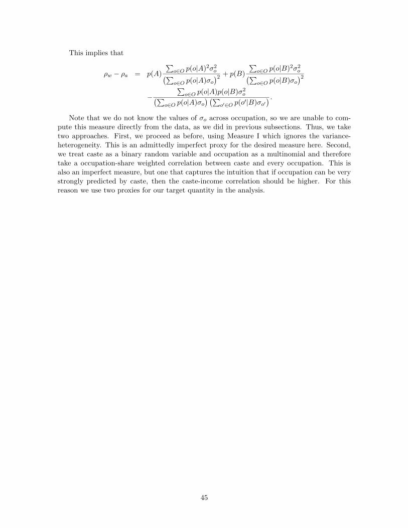
This implies that

ρw − ρa = p(A)

∑o∈O p(o|A)2σ2

o(∑o∈O p(o|A)σo

)2 + p(B)

∑o∈O p(o|B)2σ2

o(∑o∈O p(o|B)σo

)2−

∑o∈O p(o|A)p(o|B)σ2

o(∑o∈O p(o|A)σo

) (∑o′∈O p(o

′|B)σo′) .

Note that we do not know the values of σo across occupation, so we are unable to com-pute this measure directly from the data, as we did in previous subsections. Thus, we taketwo approaches. First, we proceed as before, using Measure I which ignores the variance-heterogeneity. This is an admittedly imperfect proxy for the desired measure here. Second,we treat caste as a binary random variable and occupation as a multinomial and thereforetake a occupation-share weighted correlation between caste and every occupation. This isalso an imperfect measure, but one that captures the intuition that if occupation can be verystrongly predicted by caste, then the caste-income correlation should be higher. For thisreason we use two proxies for our target quantity in the analysis.

45

C Supplementary Tables

Table C.1: Association between network density measures and measures of rainfall variabilityand within-caste income correlation

(1) (2) (3) (4) (5) (6)Income Correlation 0.368 0.207 0.145 0.235 0.208 0.173

(0.149) (0.148) (0.151) (0.098) (0.088) (0.113)[0.006] [0.24] [0.462] [0.002] [0.024] [0.092]

Income Variability -0.070 -0.013 -0.260 -0.062 -0.118 -0.270(0.157) (0.157) (0.058) (0.174) (0.163) (0.049)[0.668] [0.974] [0.002] [0.786] [0.572] [0.003]

District FE N Y Y N Y YSubdistrict FE N N Y N N YR-squared 0.1384 0.4206 0.6769 0.0747 0.4293 0.6875

Measure I Measure II

Notes: Outcome variable is the inverse of the average degree. Outcome variables and regressors scaled bytheir standard deviations. Columns (1-3) use Measure I of the caste-income correlation, whereas columns (4-6) use Measure II. Specifications include control for caste composition: p(1-p), where p is share in highcaste. Wild clustered bootstrap standard errors are presented in (.), using Rademacher weights. The clusteris at the subdistrict level, of which there are 12. 1000 samples are used per bootstrap. p-values from theWild clustered bootstrap t are presented in [.].

46

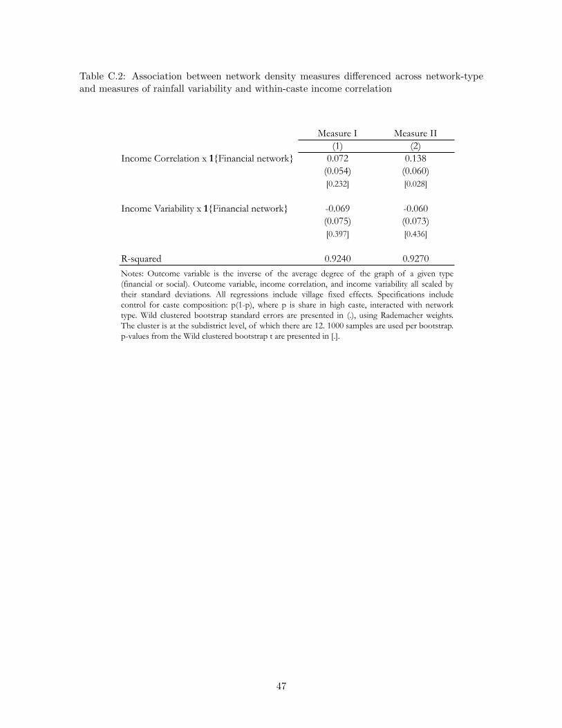
Table C.2: Association between network density measures differenced across network-typeand measures of rainfall variability and within-caste income correlation

Measure I Measure II(1) (2)

Income Correlation x 1Financial network 0.072 0.138(0.054) (0.060)[0.232] [0.028]

Income Variability x 1Financial network -0.069 -0.060(0.075) (0.073)[0.397] [0.436]

R-squared 0.9240 0.9270Notes: Outcome variable is the inverse of the average degree of the graph of a given type(financial or social). Outcome variable, income correlation, and income variability all scaled bytheir standard deviations. All regressions include village fixed effects. Specifications includecontrol for caste composition: p(1-p), where p is share in high caste, interacted with networktype. Wild clustered bootstrap standard errors are presented in (.), using Rademacher weights.The cluster is at the subdistrict level, of which there are 12. 1000 samples are used per bootstrap.p-values from the Wild clustered bootstrap t are presented in [.].

47

Table C.3: Association between average within-caste centrality of nodes with cross-caste linksand measures of rainfall variability and within-caste income correlation

(1) (2) (3) (4) (5) (6)Income Correlation x 1Financial network -0.125 -0.095 0.024 -0.421 -0.427 -0.333

0.083 0.041 0.075 0.094 0.086 0.104[0.156] [0.029] [0.818] [0.002] [0.036] [0.002]

Income Variability x 1Financial network 0.290 -0.215 -0.146 0.093 -0.131 -0.2370.206 0.409 0.211 0.123 0.161 0.132[0.212] [0.54] [0.544] [0.534] [0.532] [0.084]

District x 1Financial network FE N Y Y Y Y YSubdistrict x 1Financial network FE N N Y N Y YR-squared 0.163 0.480 0.667 0.183 0.247 0.418

Myerson Centrality Eigenvector Centrality

Notes: Outcome variable is the Myerson centrality, computed using our approximation algorithm, or eigenvector centrality. Incomecorrelation given by Measure II. Outcome variables and regressors are scaled by their standard deviations. All specifications use villagefixed effects and caste composition controls. Columns 2 and 4 include district-by-network type fixed effects and columns 3 and 6include subdistrict-by-network type fixed effects. Wild clustered bootstrap standard errors are presented in (.), using Rademacherweights. The cluster is at the subdistrict level, of which there are 12. 1000 samples are used per bootstrap. p-values from the Wildclustered bootstrap t are presented in [.].

48