© Copyright JASSS

A. O. I. Hoffmann, W. Jager and J. H. Von Eije (2007)

Social Simulation of Stock Markets: Taking It to the Next LevelJournal of Artificial Societies and Social Simulation vol. 10, no. 2, 7

<http://jasss.soc.surrey.ac.uk/10/2/7.html>For information about citing this article, click here

Received: 01-May-2006 Accepted: 09-Jan-2007 Published: 31-Mar-2007

Abstract

This paper studies the use of social simulation in linking micro level investor behaviour and macro level stock market dynamics. Empirical data from a surveyon individual investors' decision-making and social interaction was used to formalize the trading and interaction rules of the agents of the artificial stockmarket SimStockExchange. Multiple simulation runs were performed with this artificial stock market, which generated macro level results, like stock marketprices and returns over time. These outcomes were subsequently compared to empirical macro level data from real stock markets. Partial qualitative as well asquantitative agreement between the simulated asset returns distributions and the asset returns distributions of the real stock markets was found.

Keywords:Agent-Based Computational Finance, Artificial Stock Markets, Behavioral Finance, Micro-Macro Links, Multi-Agent Simulation, Stock Market Characteristics

Introduction

1.1In recent years, agent-based computational finance has developed into a growing field in which researchers rely on computational methods to overcome theinherent limitations of analytic methods (LeBaron 2000). Amongst the advantages that agent-based computational models have to offer are (1) the ease withwhich it is possible to limit agent rationality, (2) the facilitation of heterogeneity in the agent population, (3) the possibility of generating an entire dynamicalhistory of the processes under study, and (4) the ease with which it is possible to have agents interact in social networks (Axtell 2000). Furthermore, agent-based computational models as a specific instance of the broader field of social simulation are well adapted to developing and exploring theories concernedwith social processes and are well able to represent dynamic aspects of change. Using these models can help to increase our understanding of the relationshipbetween micro level attributes and individuals' behaviour and macro level aggregate effects (Gilbert & Troitzsch 1999). An example of the latter would be tostudy the influences of different types of investors' behaviour on the fluctuations of asset prices as described in e.g., Takahashi and Terano (2003).

1.2Moreover, the application of multi agent models for financial markets research has been promoted by a number of empirical puzzles or stylized facts (e.g.,time series predictability, volatility persistence/clustering, and fat tails in the asset returns distribution) that are difficult to explain using traditionalrepresentative agent structures (LeBaron, Arthur, & Palmer 1999). The latter structures assume rational agents who make optimal investment decisions andhave rational expectations about future developments (Hommes 2006). In addition, using the representative agent assumes that the choices made by all thediverse agents in a sector — e.g., consumers, investors, or producers — can be considered as the choices of one "representative" standard utility maximizingindividual whose choices coincide with the aggregate choices of the heterogeneous individuals. However, this reduction of the behaviour of a group ofheterogeneous agents is criticized as not simply being an analytical convenience but as being unjustified and leading to conclusions that are usuallymisleading and often wrong (Kirman 1992).

1.3An excellent overview of early and influential models in agent-based computational finance is given by LeBaron (2000; 2005). These models range fromrelatively simple models like the one of Lettau (1997) to very complicated models like the Santa Fe Artificial Stock Market (Arthur, Holland, LeBaron, & Palmer1997; LeBaron et al. 1999). It is beyond the scope of this paper to discuss them all in detail here, but for those unfamiliar with them, we have provided asummary in appendix 1.

1.4The myriad number of different agent-based models that are applied in finance makes this a complex research field. To even further complicate matters,finance itself is not a uniform entity. Rather, the finance literature distinguishes two fields, which are related, but differ in their main axioms and principles.These fields can be called "traditional finance" versus "behavioural finance", respectively.

1.5Traditional finance literature is based on the assumption of rational and omniscient investors who optimize the risk/return profile of their portfolios (Olsen1998). This approach has merits in the development of theoretical foundations like the Capital Asset Pricing Model and the Arbitrage Pricing Theory for astylized world with efficient markets. However, treating investors as being utility optimizing, omniscient, and unboundedly rational individuals, sets limits tounderstanding and explaining real-life investors' behaviour. The limitations of traditional finance are well-known in the field of behavioural finance and theextant literature in the latter field has contributed to understanding many facets of both micro level individual investor as well as macro level stock marketbehaviour that were inexplicable from a traditional finance perspective (for a brief overview of behavioural finance, see e.g., Nofsinger (2002), Schleifer (2000),and Shefrin (2002). However, the connections between micro level investor behaviour and macro level stock market (price) dynamics — which are an essentialpart of the artificial stock market that will be presented in this paper — remain an underdeveloped field of research according to Van der Sar (2004: 442). Withrespect to this topic, he argues in his review of behavioural finance that:

there still is a gap to be bridged between the individual investor and the market, and the question of aggregation has not been settled yet. (Vander Sar 2004: 442)

1.6Traditional finance has a long history and the majority of the agent-based computational models mentioned in previous sections and that are discussed in theliterature as outlined in appendix 1 — either explicitly or implicitly — spring from this history. Consequently, unlike the literature on agent basedcomputational finance in general, the literature on agent-based computational behavioural finance is still scarce. Takahashi and Terano (2003) are amongstthe first who explicitly aim to apply behavioural finance theories in agent-based computational models.[1] These authors state, that the decision-making rulesof investors based on behavioural finance are much more complicated than the ones in traditional finance. Moreover, they note that it is difficult to analyticallyderive asset prices under these assumptions which motivates their choice to use an agent-based model (Takahashi & Terano 2003: 2). However, they alsocritically observe that most research in artificial markets makes the micro level agent rules as simple as possible in accordance with Axelrod's "Keep It Simple,Stupid" principles (1997). Takahashi and Terano (2003) furthermore argue that this results in rules that are sometimes too mechanical and emphasize thatthese micro level rules are different from investors' behaviour in real markets. It is stated, that one of the novelties of their paper is that their models ofbounded rational agents are grounded in real theories, such as those of trend chasers, overconfident investors and the Prospect Theory as introduced byKahneman and Tversky (1979). Another novelty these authors claim to introduce is that they analyze, based on their investor models, how the behaviour ofeach investor type (i.e. fundamentalists, trend chasers and overconfident investors) are associated with overall asset price fluctuations.

1.7

This paper of Takahashi and Terano (2003) is an important step forward in explicitly applying behavioural finance theories and concepts in agent-basedmodels and argues with good reason for agent rules that are more thoroughly based on theoretical work. Notwithstanding the contribution of these authors,we consider our paper and the artificial stock market model we present, to be both novel and to offer a number of contributions to the field.

1.8The first contribution is that our model — like the model of Takahashi and Terano (2003) — is explicitly based on real theories. However, in contrast to theseauthors, we apply a multi-disciplinary approach, in which (behavioural) finance, social-psychological and consumer behaviour theories are used incombination. Amongst the theoretical concepts that are used in developing this model is the general notion of boundedly rational investors as propagated bythe behavioural finance literature (Schleifer 2000; Nofsinger 2002; Shefrin 2002) as well as more specific concepts like the Prospect Theory of Kahneman andTversky (1979). Other theories that are utilized are theories on the different personal needs people may strive to satisfy (Maslow 1954; Max-Neef 1992),conformity behaviour (Burnkrant & Cousineau 1975; Bikhchandani, Hirschleifer, & Welch 1998; Cialdini & Trost 1998; Cialdini & Goldstein 2004), and the waydecision-makers deal with uncertainty and risk (Knight 1921; Tversky & Kahneman 1974; Taylor 1974; Mitchell 1999). Moreover, theories on different socialnetwork topologies and the interactions within these networks are used in developing the model (Wellman & Berkowitz 1997; Newman 1999; Barabasi 2002).

1.9The second contribution lies in the fact that we not only based the model on the theories as introduced in the previous section, but furthermore, using thesetheories, we developed specific hypotheses with respect to the individual investors' trading and interaction behaviour and performed empirical studies in whichthese hypotheses were tested. In Hoffmann, Von Eije, and Jager (2006), we report on part of the results of these studies in which we investigated e.g., to whatextent individual investors have needs that deviate from a risk/returns perspective. Moreover, differences in the amount of investment-related knowledge andexperience of these investors were studied. Furthermore, the effect of these differences — which result in different levels of confidence — on the conformitybehaviour of these investors was examined. In the empirical studies it was found, that individual investors do have other, more social needs apart from theirfinancially oriented needs. In fact, investors that gave a higher importance to social needs and/or who had lower levels of investment-related knowledge andexperience, displayed more informational and normative conformity behaviour. Informational conformity behaviour is the expression of an individual'stendency to accept information from others as evidence about reality (Deutsch & Gerard 1955). This is expressed by e.g., asking the members of one'sreference group for information and subsequently using this information in one's own decision-making. Normative conformity behaviour is the expression ofan individual's desire to comply with the positive expectations of others (Deutsch & Gerard 1955). This expression of compliance takes the form of e.g.,performing similar actions as the individuals to whose norms one wishes to conform.

1.10Subsequently, the results of these studies have been used to develop empirically plausible agent trading and interactions rules and to parameterize the modelin order to achieve an artificial stock market that is a closer match with reality than existing models. In case we were unable to collect data to empiricallyground a model part, we conformed to well-accepted trading and behavioural principles as reported in the agent-based computational finance literature orrelied on information provided by investment practitioners like investment consultants and brokers. In the section where the model will be described, we willmake explicit how and where empirical findings have been incorporated in the model, and where we adhered to the agent-based computational financeliterature's "best practices". Moreover, more (technical) details on how the empirical findings are incorporated in the artificial stock market will be presentedthere.

1.11The third and last contribution is that we not only investigate how the aggregation of micro level investor behaviour results in macro level stock market results,but we will also estimate the empirical plausibility of the macro level stock market price and returns data that are generated by the model in the spirit ofLeBaron (1999). Yet, we will go one step further by not only investigating the occurrence of possible stylized financial market facts (Cont 2001) in the model'sreturns time series, but also determining the extent to which the stylized financial market facts in the returns time series of the simulation experiments agreewith those of a representative empirical stock market. In this case, we will compare the returns time series of our artificial stock market, that uses empiricaldata of Dutch investors, with the returns time series of the overall Dutch stock market using several statistical techniques.

1.12In this paper, we introduce the artificial stock market SimStockExchange™ (from here on "SSE") by outlining the main design of this model. Moreover, we reporton a number of simulation experiments and a first comparison is made between the results of the SSE and those of real stock markets. The remainder of thispaper is organized as follows. In section 2, the SSE model will be presented. In section 3, the results of two typical simulation runs of the SSE using twodifferent network types as well as empirically valid parameter settings for the agent rules are presented and subsequently compared to those of the overallDutch stock market. Section 4 concludes, outlines the limitations of the current paper, and discusses perspectives for related future research.

The SSE

2.1We built an artificial stock market called SSE on a personal computer using a multi agent social simulation approach. The program is written in Java and boththe Eclipse and Repast software packages are used in developing, error-testing and running the model. To succinctly show how the model works, we haveincluded a brief sample of the model's pseudo code in appendix 2. Two versions of the simulation are available for downloading: a stand-alone executableversion of the model suitable for Windows computers, SSE.exe, and a Java archive, SSE.jar that requires Java to be available on the computer and is for Linuxand MacOS. There is also a manual.

2.2The SSE is capable of simulating markets with any desirable number of investors. In the SSE, different types of investors exist who conduct transactions basedon the investment rules that are formalized for each type. At the beginning of each simulation run, each investor agent is allocated a number of stocks in itsportfolio as well as a cash budget. The investors can decide to invest all or part of their budget or to keep all or part of their budget in cash. Investors that areso unsuccessful that they lose their entire budget, are declared bankrupt by the SSE. The SSE offers the possibilities of either replacing these bankrupt agentsby similar new agents or to let them remain bankrupt and let them no longer participate in the market interactions of the model. In the simulation experimentsof this paper, bankrupt agents are replaced.

2.3The SSE operates in the following four steps: (1) every investor in the market receives a personal signal (information on the next period's expected price) andobserves the current market price, (2) depending on the confidence of the investor, the personal signal is weighted to a greater or lesser extent with the signalthat neighbouring agents have received, and based on this an order is forwarded to the stock market, (3) a new market price is calculated based on thecrossing of orders in the SSE's order book, and (4) the agent's rules can be updated according to their results. In the following sections, the SSE will beexplained in more detail.

Step 1: news enters the stock market

2.4Each time period t, investors observe for a stock s a current market price Pst (which is the same for every investor) and they also have an expectation of thenext period's price Est (which may differ among investors). The expectation of the next period's price is based on news that enters the market. Although thereis an important body of literature on the impact of different types of news on the stock markets, like announcements on company takeovers (see e.g., Keownand Pinkerton 1981), announcements on quarterly earnings (see e.g., Bernard and Thomas 1989), and announcements of stock splits (see e.g., Fama, Fisher,Jensen and Roll 1969), this literature provides little information on how one could actually model a news arrival process in an artificial stock market.Nevertheless, the literature seems to agree that one important feature of such a news arrival process would have to be that neither fat tails, nor volatilityclustering nor any kind of non-linear dependence in the returns time series of the model is caused by the news arrival process, but rather that the occurrenceof any of these stylized financial market facts is due to the actual trading and interaction of the investors in the market (Chen, Lux, & Marchesi 2001). Inspiredby the work of Chen, Lux and Marchesi (2001: 5-6), we therefore model our news arrival process as normally distributed noise with a user-specified standarddeviation around the current price.

2.5This property of the simulation model represents the fact that in real markets, different investors get different pieces of news, process the news in differentways, and consequently differ in their valuation of shares. This process leads to differences in the prices that the investors expect for the next period. Theagents do not know that the signal they receive is random noise and therefore they are bounded in their rationality.[2]

2.6

Yet, the current formalization of the news arrival process and corresponding decision-making by the investor agents differs in one important aspect fromthose that can be observed in real markets. Agents do not take news from previous periods into account for their decision-making. Rather, the agents forgetthe information signal of the previous period at the start of each new period. However, as we will see in later sections, as the agents make their decisions,information is spread through the social network. Depending on the agent's position in the social network and the agent's moment of trading, the informationit receives within a time period will be aggregated to a greater or lesser extent. So, although there is no aggregation of dispersed information beyondsubsequent time periods, within a time period, there are processes of information aggregation.

Step 2: agents make investment decisions

2.7In every time step t, each agent has to decide how much of its budget to invest in the stock s and how much to keep in cash. To determine what proportion ofits available cash budget an agent is willing to invest in the risky asset or what proportion of its portfolio of stocks it is willing to divest, formulas 1, 2, and 3as depicted below are used. These formulas are based on the well-accepted principle in the field (see e.g., Lux 1998: 148) and references therein) of making acomparison between some kind of fundamental value and current market value, or in our case comparing the expected price of a stock with its current marketprice.

If , then this proportion is (1)

If , then this proportion is -1(2)

If , then this proportion is 1(3)

Est = Expected price for stock s at time tPst = Current market price for stock s at time t

That is, an agent weighs the deviation of the current market price from the expected price for the next period by the current market price. When the expectedprice is higher than the current price it is attractive to invest, when the expected price is lower than the current price, it is more attractive to divest. The agentsreact stronger as the expected price deviates more from the current market price.[3] Depending on the standard deviation that is chosen for the news, it wouldbe possible that the above formula returns values that would imply an agent to invest more than its current cash budget allows or to sell more stocks than ithas in portfolio. In these instances — of which the chances of occurring are extremely small using the parameter settings of the experiments that arediscussed in this paper — the proportion is limited to the agent's available cash budget and portfolio of shares as can be seen in the formula's above. So,investors are not allowed to borrow money or short-sell stocks.

2.8Agents with lower levels of confidence C in the correctness of their own signal perform risk reducing strategies (RRS) in order to come to an investmentdecision. Using regression analyses, it was found in our empirical studies that investors with lower levels of investment related knowledge and experience andwho therefore have lower levels of confidence C, perform both more informational and more normative conformity behaviour, which are two specific instancesof the more general concept of RRS. In general (see e.g., Mitchell & McGoldrick 1996), RRS may be either more individual or more socially oriented and eitherof a clarifying or simplifying kind. In table 1, a number of examples of these different types of RRS that are relevant for an investing context are displayed.

Table 1: Risk reducing strategies

Individual SocialSimplifying Use a simple heuristic, e.g., the P/E ratio

of a stock.Copy the behaviour of other investors in one's social network.

Clarifying Collect more information about the stock. Ask other investors for more information, e.g., their expectations ofthe stock value.

2.9In the SSE, the focus is on social RRS. The parameter C weights the extent to which an agent trusts on its individual signal on the expected price for the nextperiod versus the extent to which it uses information obtained from its social network. C is bounded between 0 (no confidence in the correctness of theirindividual signal, i.e. only using information from the network) and 1 (complete confidence in the correctness of their individual signal, i.e. only usingindividual information on the expected next period's price). The values for C for each individual investor that will be used in the simulation experiments of thispaper are derived from the empirical studies of Hoffmann, Von Eije, and Jager (2006). In order to be able to incorporate this empirical data in the simulationmodel, two transformations were necessary. First, for each individual respondent, the average of his or her scores on the two questions that were used tomeasure C was calculated. Second, this overall score, which was on a five-point Likert scale, was transformed to a score on a one-point scale so that we onlyhad values for C between 0 and 1. These two steps resulted in an empirically validated set of estimates of C for a group of 167 investors that subsequentlycould be loaded into the model.

2.10The SSE also offers the possibility to use different distributions, e.g., uniform and normal distributions, as well as fixed values of the level of confidence C incase one would like to perform other experiments. The experiments presented in this paper, however, uses a replication of the distribution of C as found in theempirical study, based on the empirically derived estimates of C as found for each individual investor.

2.11The extent to which an agent uses a clarifying versus a simplifying strategy is weighed by a parameter named R (risk reducing strategy). R is bounded between0 (only using a clarifying strategy) and 1 (only using a simplifying strategy). The values for R that will be used in the experiments are derived from theempirical studies in the following way. First, for each individual respondent, we calculated his or her average score for his or her propensity to use clarifyingstrategies Sc, which was measured using two questions, and their propensity to use simplifying strategies Ss, which was measured using three questions.Second, we again transformed these overall scores — which were measured on a five-point Likert scale — to a score on a one-point scale, so that we also hadvalues for Sc and Ss between 0 and 1. Third, in order to convert these two scores to one value for R that indicated the relative importance of either of these twotypes of strategies, we used the following formulae:

If , then (4)

If , then (5)

These three steps resulted in an empirically validated set of estimates of R for a group of 167 investors. A schematical overview of the above is given in figure1 below. Although in this overview, only the extreme situations (C = 0, C = 1, R = 0, R = 1) are displayed, investors in our model can also trust partly on theirown signal and partly on information obtained from their social network (0 < C < 1) and use a combination of both clarifying and simplifying strategies (0 < R< 1) as can be seen in appendix 3.

2.12In case one would like to perform other experiments, the SSE also offers the possibility to use different distributions, e.g., uniform and normal distributions, as

well as fixed values with regard to the relative proportion R of using clarifying versus simplifying strategies. The experiments presented in this paper, however,only use the empirically derived set of estimates of R as found for the individual respondents.

2.13In appendix 3, the empirically derived values as well as sample statistics for C and R for the before discussed sample of investors are displayed in a table.

Figure 1. Simplified overview of the SSE agents' trading behaviour

2.14The previously introduced clarifying strategy is a form of informational conformity behaviour. When performing this strategy, the agent asks other agents in itssocial network to which it is connected by a single link what prices they expect for the next period and calculates the unweighted average of theseexpectations.[4] Subsequently, the agent will weigh the value of its individual signal of the expected next period's price and the signal of the next period'sexpected price obtained from its social network by its value for C (confidence). For example, if an agent's value for C is 0.2, the agent will weigh its ownexpectation for 20% and the expectation obtained from the social network for 80%.

2.15The previously introduced simplifying strategy is a form of normative conformity behaviour. When performing this strategy, the agent will perform similaractions as the agents in its social network to which it is connected by a single link. The agent observes the investment behaviour of its neighbours andevaluates whether there are more selling or more buying agents. It will decide whether to buy or to sell depending on what action is dominant among itsneighbours. After it has identified the dominant action, it will conform to this action. In order to decide how many shares to buy or to sell, the agent will takethe average value of the expectations of the next period's price of the group of investors (either buyers or sellers) it decided to copy. Then, it again weighs thisaverage value with its own expectation according to its level of confidence (C) to arrive at an average expected value for the next period's price. This value issubsequently used to arrive at the decision how much of its remaining cash budget or stock portfolio to invest or divest. When the number of buyers andsellers in the market is equal, the investor will simply take the average of all their expectations of the next period's stock price and weigh this with its ownexpectation to arrive at a decision. In this one and exceptional case, the decision is thus made in a similar way as in the clarifying strategy.

2.16All agents in the SSE are connected to each other in a social network. Depending on this social network topology, agents differ in the number of other agentsto which they are connected and information on the expectations of the next period's stock price diffuses in different ways and at different speeds through thesocial network. This may give some agents an informational advantage in comparison to other agents in the social network.

2.17In every time step, all agents receive news at the same time, but the order in which the agents are allowed to decide to trade and forward their order to theorder book, is random. So, depending on whether an agent is amongst the first or last agents which are selected to trade, the information this agent collectsfrom its direct neighbours may already contain information that these neighbours have collected from their neighbours and the neighbours' neighbours fortheir decision-making or not. Notwithstanding this simplification, different social network topologies will vary in their information diffusion characteristics(Cowan & Jonard 2004). In order to investigate to what extent the stock market returns time series' dynamical features are affected by these differences, wecompare in our simulation experiments the results of two different network topologies. The network topologies that we use are the torus network (regularlattice) and the Barabasi and Albert (1999) scale free network. A torus network is simply a lattice whose edges are connected, and a scale free network is anetwork in which the distribution of the connectivity of the nodes of the network follows a power law, i.e. there are many nodes with only a few connections toothers, and there are only a few nodes with many connections to others. Many networks in real life, like those of web pages on the Internet and scientificcitations, behave like a scale free network and also have small world characteristics (Watts & Strogatz 1998; Barabasi & Albert 1999; Amaral, Scala, Barthelemy,& Stanley 2000; Barabasi 2002; Buchanan 2002).

2.18Figures of the two different network topologies that are used in the experiments are displayed in figure 2 and figure 3, respectively.

Figure 2. Torus network

Figure 3. Barabasi and Albert scale free network

Step 3: a new market price is calculated

2.19To determine the market price, an order book is used to which agents forward their orders that either consists of a maximum price and the number of stocksthat the agent wishes to buy for this price or a minimum price and the number of stocks the agent is willing to sell for this price. The general rule is that theprocessing of orders follows the FIFO (first in, first out) principle and in the situation that it is not possible to cross a complete order, an order can be partlyexecuted.[5] The non-executed part of the order remains in the order book until it is (1) eventually crossed by another order or (2) the respective agentdecides to issue a new order.

Buying stocks

2.20The maximum price that buying agents are willing to pay for their shares is the price they expect for the next period. At prices lower than this expectation,these agents expect to gain money. At prices higher than their expectation, the agents expect to lose money. This maximum price is used to determine thenumber of shares the investor wants to buy. This is done by dividing the budget to invest by the expected price for the next period, rounded off downward tothe closest whole number. So, each buying investor forwards a limit order to the market stating the number of shares it wants to buy and the limit price that itis willing to pay for these shares. In case its limit order crosses another agent that is willing to sell the requested number of shares at the indicated limit price,the order is executed and removed from the order book. In case the order crosses another agent that is willing to sell at a price below the limit, the order isexecuted for the average of the bid and ask price. This system of "splitting the difference" is inspired by Beltratti and Margarita (1992). In case there is noagent willing to sell at the limit order price of the agent, the order stays in the order book until it eventually crosses another ask order or the agent issues anew order, in which case the old order is deleted from the order book.

Selling stocks

2.21The minimum price selling agents are willing to sell their shares for is the price that they expect for the next period. For them it is no problem to sell belowthe current price, as they expect the price in the next period to (downwardly) move towards their own expected price, which is lower than the current price. Aslong as the selling price is above the expected price for the next period, these agents expect to minimize their loss. However, they will not sell for less thanthe price they expect for the next period. So, these agents calculate the number of shares they want to sell as the budget they want to sell divided by theexpected price for the next period, also rounded off downward to the nearest whole number. In case this limit order crosses another agent that is willing tobuy the offered number of shares at the indicated limit price, the order is executed and removed from the order book. In case this order crosses another agentthat is willing to buy at a price above the limit, the order is executed for the average of the ask and bid price. In case there is no agent willing to buy at thelimit order price of the agent, the order stays in the order book until it finally crosses another bid order or the agent issues a new order, in which case the oldorder is deleted from the order book.

The market price of stocks

2.22The market price that is realized in each time step is calculated as the average of the bid and ask prices that are present in the order book, weighted by thenumber of asked and offered shares. In this way, we account for the price pressure that is put on the market by the bid and ask orders. Even when not all theorders are executed, they still influence the market sentiment and therefore the price level.

2.23Although in the simulation experiments described in this paper, only the shares of one stock are traded amongst the investor agents, the SSE offers thepossibility to incorporate a number of different stocks.

Step 4: updating the agents' rules

2.24Most if not all artificial stock market models, including the SSE, have a feedback loop from the macro to the micro level in the sense that the individual agent'sorders are influenced by an aggregate variable such as the stock price. This type of feedback effect can be characterized as feedback influencing the input thatis used in the decision-making of the individual agents. However, this type of feedback does not change the way in which the agents make their decisions.Investors for example do not change the type of strategy they use, only the input that is used to determine e.g., the type of order (buy or sell) and the ordersize, is affected. A general point of critique on these type of models made by e.g., Arthur (1995) is therefore that the market dynamics are generated by theactions of the investors, but the cognition of the investors is never affected by the evolution of the market. One of the contributions of the SSE is that we haveincorporated the possibility to include a feedback mechanism that influences the decision-making of the investor. Investors can change their strategiesaccording to the returns they get. Using this updating mechanism, the rules which the agents use depend on their successfulness. Agents with higher returns,who are more successful, get higher levels of confidence C in the correctness of their own signal and therefore in the correctness of their own rules. Yet, itshould be noted, that with the current formalization of the news arrival process, there is little in these news signals — except from the variance — that couldmake decisions based on them more or less effective than other agents' decisions. Since agents cannot "choose" this variance themselves, the currentformalization of the model gives little room for the agents' decisions to be improved consistently. In future versions of the model, experiments could beperformed with news arrival processes using other distributions, giving more learning opportunities for the agents and so the possibility to create trulysuperior strategies that provide these agents with consistently higher payoffs.

Experiments

3.1Using the settings for both C and R as were empirically found for 167 investors, the experiments that will be discussed in this paper compare the time seriesbehaviour of the simulated price and returns series in two different network situations, a torus network and a scale free network.[6] Due to the superiorinformation diffusion characteristics of the latter, we expect random shocks (news in the form of random noise) to dampen out more quickly and thereforeexpect these networks to display less volatility clustering than networks with poorer information diffusion characteristics, like the regular torus network.

3.2An overview of the settings of the two simulation experiments is shown in table 2 below.

Table 2: General parameter settings

Parameter description Experiment 1 Experiment 2Number of agents 167 167Initial wealth of agents 100 100Bankrupt agents Are replaced Are replacedNetwork type Torus Scale free networkNews distribution Normal NormalNews average μ 0 0News standard deviation σ 0.020 0.020News frequency Every time step Every time stepNumber of stocks 1 1Number of time steps 929 929Initial number of stocks in portfolio 10 10Initial stock price 10 10Updating of confidence of agents according to their returns Yes YesLevel of confidence C See appendix 3 See appendix 3Risk Reducing Strategy R See appendix 3 See appendix 3Seed to generate network 1159791325531 1159791325531

3.3To generate the time series of both experiments, the market was initially run for 500 time steps to allow eventual early transients to die out. Subsequently, themarket was run for another 929 time steps for which the returns time series were calculated. The value of 929 time steps was chosen to accommodate withthe availability of data on the real stock market that would be used as a benchmark. In order to avoid problems of missing data due to weekends, holidays, andother special occasions, we decided to use weekly data. This resulted in 929 observations for the overall Dutch stock market from the seventh of January of1987 until the twentieth of October 2005.[7]

3.4In figures 4 through 7 and 8 through 11, the price and returns time series, returns distribution and autocorrelation graphs for experiment 1 and 2 with thetorus network and the scale free network, respectively, are shown. Figures 12 through 15 show the same weekly information for the overall Dutch stockmarket.

Figure 4. Price time series experiment 1 (torus network)

Figure 5. Returns time series experiment 1 (torus network)

Figure 6. Returns distribution experiment 1 (torus network)

Figure 7. Autocorrelation graph of the returns of experiment 1 (torus network)

3.5The impression given by figure 4 and figure 5, although it is more difficult to notice in the latter figure, is that the price swings in the market "arrive inclusters". Periods of relative tranquillity in which the price changes remain small are alternated by periods of increased volatility with larger price changes.Volatility clustering in the returns time series of this experiment, as can also be observed in real stock markets, is therefore expected to be present in theresults of this first experiment. However, more thorough statistical analyses like GARCH (1,1) estimates are necessary to prove this to be actually the case. Intable 3, one can find the results of such a GARCH model.

3.6Evaluating figure 6 suggest the returns distribution of the first experiment to be relatively close to a normal distribution, while more formal results on this arealso presented in table 3.

3.7Figure 7 shows significant linear autocorrelation in the returns for many lags. In general, weekly and monthly data on real stock markets have also been foundto exhibit linear autocorrelation (Cont 2001) and it can be seen in figure 15, that the weekly returns of the overall Dutch stock market also show significantautocorrelation for many lags. For more high frequency data, like hourly or daily stock data, no significant linear autocorrelation in both price increments andasset returns are reported (Fama 1970; Pagan 1996). Absence of autocorrelation means that it is impossible to consistently achieve positive expected earningswith a simple strategy that uses statistical arbitrage. An investor cannot be expected to be able to predict tomorrow's stock prices or asset returns usingtoday's stock prices or asset returns data. This can be seen as support for the efficient market hypothesis (Fama 1991). However, as stated above, it has beenproven (see e.g., Cont 2001) that when the time scale on which the linear autocorrelation is measured is increased to e.g., weekly data, this absence ofautocorrelation does not systematically hold anymore.

Figure 8. Price time series experiment 2 (scale free network)

Figure 9. Returns time series experiment 2 (scale free network)

Figure 10. Returns distribution experiment 2 (scale free network)

Figure 11. Autocorrelation graph of the returns of experiment 2 (scale free network)

3.8It is difficult to detect systematic differences between the two experiments when comparing figures 4 through 6 with figures 8 through 10. On first sight, onemight be led to believe, that the price and returns time series of the experiments performed with the two different social network topologies display rathersimilar characteristics. Only when comparing the autocorrelation graphs of figures 7 and 11, a clear distinction between both experiments appears. While thereturns of experiment 1 (torus network) show significant autocorrelation in 17 lags, this is only true for 9 lags in experiment 2 (scale free network). Usingstatistical tests makes it is easier to detect systematic differences between the results of experiment 1 and 2. The results of such tests are depicted in table 3.

Figure 12. Price index time series overall Dutch stock market 1987~2005

Figure 13. Returns time series overall Dutch stock market 1987~2005

Figure 14. Returns distribution overall Dutch stock market 1987~2005

Figure 15. Autocorrelation graph of the returns of the overall Dutch stock market 1987~2005

Table 3: Summary statistics of experiment 1, 2, and the overall Dutch stock market

Description Experiment 1: torus network

Experiment 2: scale free network

Dutch Stock Market

Std. σ 0.051 0.063 0.025Kurtosis 3.149 2.919 8.466Durbin Watson Statistic 2.184 2.117 2.194

Coeff. Prob. Coeff. Prob. Coeff. Prob.Jarque-Bera 7.795** 0.020 4.819 0.090 1262.518* 0.000

Conditional Variance EquationExperiment 1: torus network

Experiment 2: scale free network

Dutch Stock Market

Coeff. Prob. Coeff. Prob. Coeff. Prob.C 0.000 0.9000 0.001 0.718 0.002* 0.000Residuals (-1)^2 (ARCH) 0.015 0.511 0.061 0.156 0.148* 0.000GARCH (-1) 0.827* 0.004 0.078 0.895 0.828* 0.000

Values marked with an asterisk ( * ) are significant at the 0.01 level.Values marked with two asterisks (**) are significant at the 0.05 level.All statistics are performed on the continuously compounded returns as a perunage (i.e. returns t1 = ln (pt / pt-1 )).

Table 3 reports on the results of a number of common statistical tests performed on the overall market returns time series of both experiments and of theweekly returns data of the overall Dutch stock market.

3.9The first row shows the volatility of the returns time series as defined by the standard deviations of the returns for the two simulation experiments as well asfor the overall Dutch stock market. The standard deviation of the news in the two experiments was set at 0.02, a value close to the standard deviation that canbe observed in the returns time series of the overall Dutch stock market. However, both experiments show a higher variability in the returns time series thanthe before mentioned 0.02 and the difference between the two cases is relatively small. Social interaction amongst investors in the SSE is a possible reason forthis increased level of the variability. Investors partly reacting on news and partly reacting on each other might create self-reinforcing dynamics, therebypushing the standard deviation of returns to higher levels than can be justified by the news that hits the market only.

3.10The second row shows the kurtosis of the simulation experiments as well as that of the overall Dutch stock market. The two simulation experiments show akurtosis that approximates that of a normal distribution — which has a kurtosis of 3.00 — while the empirical stock market shows a significant amount ofexcess kurtosis, which can also be seen in figure 14. The returns distribution in the overall Dutch stock market is leptokurtotic; a pattern that is common forreal asset returns distributions. Using the parameter settings from table 2, the SSE does not replicate this empirically found fact. This can be explained fromthe fact, that the news generation process in the SSE currently is based on a normal distribution. As argued in a previous section, this was a necessarysimplification as the literature provides no information on how one could incorporate real-life news arrival processes in a model.

3.11The third row shows the Durbin Watson statistic, testing for autocorrelation in the residuals.[8] We can observe from table 3, that the two simulationexperiments take on test values between 2.12 and 2.18, which lines up well both qualitatively and quantitatively with the test value of 2.19 as found in theempirical stock market. These values indicate, that both the two simulation experiments as well as the overall Dutch stock market display a very small amountof negative autocorrelation.

3.12The next row shows the coefficients and probabilities of the Jarque-Bera test, which is a goodness-of-fit measure of departure from normality which is basedon both the sample kurtosis and skewness (Bera & Jarque 1980; 1981). When the coefficient of this test is significant, the returns time series depart fromnormality, and the higher the value of this coefficient, the greater the departure from normality. As can be seen in table 3, the returns distribution of theoverall Dutch Stock Market strongly departs from normality, while the returns distribution of the first experiment (torus network) do so to a lesser extent. Thereturns distribution of the second experiment (scale free network) do not significantly deviate from normality.

3.13The next three rows show a common test in finance for volatility persistence or "volatility clustering", namely the (Generalized) ARCH test.[9] A typical patternobserved for real asset returns is that the coefficients on all three terms in the conditional variance equation are highly statistical significant, with a small valuefor the variance intercept term C, a somewhat larger ARCH term, and an even larger GARCH term. The ARCH term represents the lagged squared error, whilethe GARCH term represents the lagged conditional variance. For real asset returns, both terms summed together are generally found to be close to unity. Thisindicates that shocks to the conditional variance will be highly persistent, i.e. there is volatility persistence. Qualitatively, the results of both simulationexperiments line up relatively well with the empirical stock market with regard to the relative proportions of the three terms of the conditional varianceequation. Only in the first experiment, however, we observe a statistically significant GARCH term that also lines up well quantitatively with the terms found inthe real asset returns of the overall Dutch stock market. For experiment 2, with the scale free network, none of the terms in the conditional variance equationis statistically significant, while experiment 1, with a regular torus network, displays a highly significant GARCH effect. So, for these two experiments, weobserve ceteris paribus that in artificial stock markets with scale free networks, there is no statistically significant proof of volatility clustering, but artificialstock markets with a torus network do display volatility clustering. A possible explanation for this is that the superior information diffusion capacities of thescale free network facilitate an immediate absorption of the news by all network members and inhibit news shocks of yesterday to have much effect on today'sreturns. Moreover, one could argue that in spite of today's ubiquitous information through e.g., mass medial devices and the Internet, which have lowered thecost of information drastically, and despite the fact that theoretically and empirically there is a good case for the society as a scale free network, in reality (at

least for the investing population of society) the society is more likely to behave like a torus network with regard to the information diffusion capacities, whereinformation sometimes takes long to travel to remote corners of the network and shocks of the past continue to influence the present for a considerable periodof time.

Conclusions and Limitations

4.1In this study we have presented the SSE and given a practical example of the possible combination of empirical micro and macro level data, theoretical microand macro level perspectives, and a multi-agent based social simulation approach in the development of an artificial stock market. It was shown, how artificialstock markets can be used to explore how different micro level behavioural processes aggregate to macro level phenomena and, in turn, how these aggregatedoutcomes affect individual investors' behaviour. In the SSE, investor agents make investment decisions using empirically estimated decision rules and sociallyinteract in different social network structures. From these market interactions, macro level price and returns time series result, which are subsequentlycompared to empirical macro level data. First comparisons showed limited qualitative and quantitative resemblances of the simulated data with the real dataand therefore a number of opportunities to improve this fit. In the following, we will outline a number of limitations of the current study, which provideopportunities for future research and which are expected to improve the fit between the results of the model and the real world when they would be overcome.

4.2First, the artificial stock market SSE that was presented in this paper, remains a model and therefore a simplified reproduction of reality. Especially the questionon how one should model the news arrival process poses a number of difficult questions which are hard to overcome for a modeller of an artificial stockmarket. It is precisely this difficulty, and the chances to be heavily criticized for the way one models the news arrival process if one does try to incorporatesuch a process, that can be understood as a rationale for many modellers in agent-based finance to omit news arrival processes from their artificial stockmarkets altogether (Lux 2006). We, however, have chosen to model the news arrival process in a simplified way as normally distributed noise around thecurrent price, which forms a limitation of the current study but poses a challenge for future research.

4.3Second, the respondents from the empirical studies that were used to formalize the agents' trading and interaction rules, were mainly individual investors,although a small percentage (approximately 5%) of the respondents indicated to be either a professional investor, a broker or to work at a large investmentcompany. It could be argued, that in reality, large institutional investors are the main determinants of price dynamics and therefore the composition of oursample represents a limitation.[10] There are a number of reasons, why we expect the implications of this possible limitation to be limited. First, individualinvestors constitute an important group in the financial marketplace and their decision-making behaviour is likely to have an impact on the stock market as awhole (De Bondt 1998). The latter argument becomes even more pronounced taking into consideration that even a small country as The Netherlands alreadyaccommodates 2,300,000 individual investors that invest directly and indirectly in the stock market (VEB 2002). Second, it seems safe to assume, that thestock price expectations of most large institutional investors and investment banks — who are well-connected to the most important stock analysts — arepredominantly of the correct magnitude. This would imply that most market disturbances are caused by individual investors and that the large institutionalinvestors merely form a stable force in the market that has to react to or is affected by disturbances caused by individual investors. This makes it highlyinteresting and relevant to investigate the effect of different types of individual investors on the stock market dynamics.

4.4Third, the empirical benchmark in this study was the overall Dutch stock market, rather than specific shares of a company that are traded on this market. Weexpect important differences between the time series behaviour of specific companies and that of the aggregate market. It seems a realistic assumption, thatcertain shares are traded more by investors with a low confidence or who are highly socially oriented and other shares are traded more by high confidence,experienced investors who are only interested in certain fundamental characteristics of the company and make their decisions in a more individual way. Infuture research, we plan to compare the results of the SSE to the returns time series of several individual publicly traded companies.

4.5Fourth, the time horizons of the simulation-generated data and the real market data might be incompatible. It is not yet evaluated whether one time step ofthe simulation model with its accompanying data point is comparable to one data point in the real market data, but in future studies we intend to experimentwith different time horizons.

Acknowledgements

The authors like to thank conference participants of the First World Conference on Social Simulation WCSS 06 and the Artificial Economics 2006 Conference aswell as two anonymous referees of the JASSS for their valuable comments on this paper. This paper greatly profited from their feedback. Moreover, wegratefully acknowledge the programming assistance of Björn Lijnema. The usual disclaimer applies.

Notes

1 We note that there are authors (see e.g., Lux 1998: 148) who argue that distinguishing between groups of trend following and fundamentalist investors isalready an application of behavioral finance.

2 In the current formalization of the SSE, the latter characteristic implies that the market interactions are a zero-sum game. Furthermore, the currentformalization of the SSE features no transaction costs.

3 This mechanism can be interpreted as a form of symmetrical, linear loss aversion and is comparable to the mechanisms used in e.g. , Day and Huang (1990).It is also possible to include a more elaborate loss aversion mechanism, like the type as assumed in the prospect theory (Kahneman & Tversky 1979).Asymmetrical loss aversion types, however, call for more elaborate methods of analysis that take this asymmetry into account, like EGARCH (Brooks 2004). Foran example of the application of a loss aversion mechanism as proposed by prospect theory, see e.g., Takahashi and Terano (2003).

4 The SSE also offers other options of weighting the expectations of the agents' neighbors, like weighting the neighbors' expectations according to theimportance of their network position or their past success in investing. These options, however, are until now not researched and outside the scope of thispaper.

5 We use the in the financial literature common phrase “crossing of orders” to indicate, that a buy or sell order matches another sell or buy order, respectively,and subsequently a transaction takes place.

6As the 167 investors for which we have obtained empirical data do not constitute a social network by themselves, but rather are a sample of the overall Dutchinvestor population, the exact positions of the investor agents in the two different social networks is arbitrarily chosen. In future research, one might try torebuild an existing social network of investors and incorporate it in an artificial stock market. We have also performed the same simulation experiments, butthen creating 10 copies or “clones” of the 167 agents, resulting in 1670 agents, in order to test for the occurrence of the law of large numbers. However, theresults of these experiments are exactly the same as those of the experiments with only 167 agents

7 This was the longest time frame available from DataStream at the time of collecting the data for this article (October 2005).

8 Autocorrelation is the correlation of a process Xt against a time-shifted version of itself. The efficient markets hypothesis of modern finance literatureassumes that the residuals of today are uncorrelated with the residuals of tomorrow. That is, today's news is completely and immediately absorbed in today'sstock prices and has no effect on tomorrow's stock prices. When the Durbin Watson statistic takes on the test value of two, this corresponds to the case wherethere is no autocorrelation in the residuals. When this statistic takes on a test value of zero, this corresponds to the case of perfect positive autocorrelation inthe residuals. In case the test statistic takes on the value of four, this corresponds to the case where there is perfect negative autocorrelation in the residuals.

9 ARCH is the test for conditional heteroscedasticity as developed by Engle (1982). GARCH is a generalized model for conditional heteroscedasticity asdeveloped independently by Bollerslev (1986) and Taylor (1986).

10 We thank one of the anonymous referees for bringing this issue to our attention.

References

AMARAL, L. A. N., Scala, A., Barthelemy, M., & Stanley, H. E. (2000). Classes of small-world networks. Proceedings of the National Academy of Sciences USA, 97,11149-11152.

ARIFOVIC, J. (1996). The behavior of the exchange rate in the genetic algorithm and experimental economies. Journal of Political Economy, 104, 510-541.

ARTHUR, W. B. (1995). Complexity in Economic and Financial Markets. Journal of Complexity, 1.

ARTHUR, W. B., Holland, J., LeBaron, B., & Palmer, R. T. P. (1997). Asset pricing under endogenous expectations in an artificial stock market. In W.B.Arthur, S.Durlauf, & D. Lane (Eds.), The economy as an evolving complex system II (pp. 15-44). Reading, MA: Addison-Wesley.

AXELROD, R. (1997). The Complexity of Cooperation. Princeton: Princeton University Press.

AXTELL, R. L. (2000). Why Agents? On The Varied Motivations For Agent Computing In The Social Sciences. (Rep. No. 17).

BARABASI, A.-L. (2002). Linked. The new science of networks. Cambridge, Massachusetts: Perseus Publishing.

BARABASI, A.-L. & Albert, R. (1999). Emergence of scaling in random networks. Science, 286, 509-512.

BELTRATTI, A. & Margarita, S. (1992). Evolution of trading strategies among heterogeneous artificial economic agents. In J.A.Meyer, H. L. Roitblat, & S. W.Wilson (Eds.), From animals to animats 2. Cambridge, MA: MIT Press.

BERA, A. K. & Jarque, C. M. (1981). Efficient tests for normality, homoskedasticity and serial independence of regression residuals: Monte Carlo evidence.Economics Letters, 7, 313-318.

BERA, A. K. & Jarque, C. M. (1980). Efficient tests for normality, homoskedasticity and serial independence of regression residuals. Economics Letters, 6, 255-259.

BERNARD, V. L. & Thomas, J. K. (1989). Post-Earnings-Announcement Drift: Delayed Price Response or Risk Premium? Journal of Accounting Research, 27, 1-36.

BIKHCHANDANI, S., Hirschleifer, D., & Welch, I. (1998). Learning from the behavior of others: conformity, fads, and informational cascades. Journal of economicperspectives, 12, 151-170.

BOLLERSLEV, T. (1986). Generalised Autoregressive Conditional Heteroskedasticity. Journal of Econometrics, 31, 307-327.

BRAY, M. (1982). Learning, estimation, and the stability of rational expectations. Journal of economic theory, 26, 318-339.

BROOKS, C. (2004). Introductory Econometrics for Finance. Cambridge: Cambridge University Press.

BUCHANAN, M. (2002). Small World: uncovering nature's hidden networks. London: Phoenix.

BURNKRANT, R. E. & Cousineau, A. (1975). Informational and Normative Social Influence in Buyer Behavior. The Journal of Consumer Research, 2, 206-215.

CHEN, S.-H., Lux, T., & Marchesi, M. (2001). Testing for Non-Linear Structure in an Artificial Financial Market. Journal of Economic Behavior and Organization, 46,327-342.

CHIARELLA, C. (1992). The dynamics of speculative behavior. Annals of Operations Research, 37, 101-123.

CIALDINI, R. B. & Goldstein, N. J. (2004). Social Influence: Compliance and Conformity. Annual Review of Psychology, 55, 591-621.

CIALDINI, R. B. & Trost, M. R. (1998). Social influence: social norms, conformity, and compliance. In D.T.Gilbert, S. T. Fiske, & G. Lindzey (Eds.), The Handbook ofSocial Psychology (4 ed., pp. 151-192). Boston: McGraw-Hill.

CONT, R. (2001). Empirical properties of asset returns: stylized facts and statistical issues. Quantitative Finance, 1, 223-236.

COWAN, R. & Jonard, N. (2004). Network structure and the diffusion of knowledge. Journal of Economic Dynamics and Control, 28, 1557-1575.

DAY, R. H. & Huang, W. (1990). Bulls, bears and market sheep. Journal of Economic Behavior and Organization, 14, 299-329.

DE BONDT, W. F. M. (1998). A portrait of the individual investor. European economic review, 42, 831-844.

DEUTSCH, M. & Gerard, H. B. (1955). A study of normative and informative social influences upon individual judgment. Journal of Abnormal and SocialPsychology, 51, 629-636.

ENGLE, R. F. (1982). Autoregressive Conditional Heteroskedasticity with Estimates of the Variance of United Kingdom Inflation. Econometrica, 50, 987-1007.

FAMA, E. F. (1970). Efficient capital markets: a review of theory and empirical work. Journal of finance, 25, 383-417.

FAMA, E. F. (1991). Efficient capital markets: II. Journal of finance, 46, 1575-1617.

FAMA, E. F., Fisher, K. L., Jensen, M. C., & Roll, R. (1969). The Adjustment of Stock Prices to New Information. International Economic Review, 10, 1-21.

GILBERT, N. & Troitzsch, K. G. (1999). Simulation for the Social Scientist. Buckingham: Open University Press.

GODE, D. K. & Sunder, S. (1993). Allocative efficiency of markets with zero intelligence traders. Journal of Political Economy, 101, 119-137.

GROSSMAN, S. & Stiglitz, J. (1980). On the impossibility of informationally efficient markets. American Economic Review, 70, 393-408.

HOFFMANN, A. O. I., Von Eije, J. H., & Jager, W. (2006). Individual Investors' Needs and Conformity Behavior: An Empirical Investigation. SSRN Working Paper Series.http://papers.ssrn.com/sol3/papers.cfm?abstract_id=835426 .

HOMMES, C. H. (2006). Interacting Agents in Finance. In L.Blume & S. Durlauf (Eds.), New Palgrave Dictionary of Economics (2nd ed.). Palgrave Macmillan.

KAHNEMAN, D. & Tversky, A. (1979). Prospect theory: an analysis of decision under risk. Econometrica, 47, 263-291.

KARAKEN, J. & Wallace, N. (1981). On the indeterminacy of equilibrium exchange rates. Quarterly journal of economics, 96, 207-222.

KEOWN, A. & Pinkerton, J. (1981). Merger Announcements and Insider Trading Activity. Journal of finance, 36, 855-869.

KIRMAN, A. P. (1992). Whom or What Does the Representative Individual Represent. Journal of economic perspectives, 6, 117-136.

KNIGHT, F. H. (1921). Risk, Uncertainty and Profit. Boston, MA : Hart, Schaffner & Marx; Houghton Mifflin Company.

LEBARON, B. (2000). Agent-based computational finance: suggested readings and early research. Journal of Economic Dynamics and Control, 24, 679-702.

LEBARON, B. (2005). Agent-based Computational Finance. In K.L.Judd & L. Tesfatsion (Eds.), The Handbook of Computational Economics, Vol. II North-Holland.

LEBARON, B., Arthur, W. B., & Palmer, R. (1999). Time series properties of an artificial stock market. Journal of Economic Dynamics and Control, 23, 1487-1516.

LETTAU, M. (1997). Explaining the facts with adaptive agents: the case of mutual fund flows. Journal of Economic Dynamics and Control, 21, 1117-1148.

LUX, T. (1998). The socio-economic dynamics of speculative markets: interacting agents, chaos, and the fat tails of return distributions. Journal of EconomicBehavior and Organization, 33, 143-165.

LUX, T. (2006). Communication on the Artificial Economics 2006 Conference, Aalborg, Denmark. personal communication with the authors.

MASLOW, A. H. (1954). Motivation and personality. New York: Harper and Row.

MAX-NEEF, M. (1992). Development and Human Needs. In P.Ekins & M. Max-Neef (Eds.), Real-life economics: understanding wealth creation London/New York:Routledge.

MITCHELL, V.-W. & McGoldrick, P. J. (1996). Consumers' risk reducing strategies: a review and synthesis. The international review of retail, distribution andconsumer research, 6, 1-33.

MITCHELL, V.-W. (1999). Consumer Perceived Risk: Conceptualisations and Models. European Journal of Marketing, 33, 163-195.

NEWMAN, M. E. J. (1999). Small Worlds. The structure of social networks. Santa Fe Institute Working Paper .

NOFSINGER, J. R. (2002). The psychology of investing. Upper Saddle River, New Jersey: Prentice Hall.

OLSEN, R. A. (1998). Behavioral finance and its implications for stock-price volatility. Financial Analysts Journal, March/April, 10-18.

PAGAN, A. (1996). The econometrics of financial markets. Journal of empirical finance, 3, 15-102.

ROUTLEDGE, B. R. (1994). Artificial selection: genetic algorithms and learning in a rational expectations model (Rep. No. Technical raport, GSIA). Carnegie Mellon,Pittsburgh, Penn.

SCHLEIFER, A. (2000). Inefficient markets, an introduction to behavioral finance. Oxford University Press.

SHEFRIN, H. (2002). Beyond greed and fear. Understanding behavioral finance and the psychology of investing. Oxford University Press.

TAKAHASHI, H. & Terano, T. (2003). Agent-Based Approach to Investors' Behavior and Asset Price Fluctuation in Financial Markets. Journal of artificial societiesand social simulation, 6(3) http://jasss.soc.surrey.ac.uk/6/3/3.html.

TAYLOR, J. W. (1974). The Role of Risk in Consumer Behavior. Journal of Marketing, 38, 413-418.

TAYLOR, S. J. (1986). Forecasting the Volatility of Currency Exchange Rates. International Journal of Forecasting, 3, 159-170.

TVERSKY, A. & Kahneman, D. (1974). Judgement under uncertainty: Heuristics and Biases. Science, 185.

VAN DER SAR, N. L. (2004). Behavioral finance: How matters stand. Journal of Economic Psychology, 25, 425-444.

VEB (2002). Is beleggen uit en sparen in? Effect, 5.

WATTS, A. and Strogatz, S. H. (1998, June). Collective dynamics of 'small-world' networks. Nature, 393, 440-442.

WELLMAN, B. & Berkowitz, S. D. (1997). Social Structures: a Network Approach. London: JAI Press.

Appendix 1: overview of agent-based models in finance

A.1The framework of Lettau (1997) is an agent benchmark that implements many of the ideas of evolution and learning in a population of traders in a very simplesetting. In this setting, agents have to decide how much of a risky asset to purchase, which is sold at a price p and which issues a random dividend d that ispaid in the next period. There are two main simplifications in this framework: the price is given exogenously and the agents are assumed to have myopicconstant absolute risk aversion preferences. The objective of Lettau is to investigate how close evolutionary learning mechanisms can get to the optimalsolution in deciding how much of the risky asset to hold in comparison to the risk free bond paying zero interest. The results of this framework demonstratethat the genetic algorithm is able to learn the optimum distribution between the risky asset and risk free bond, but is biased towards holding more of the riskyasset.

A.2The framework of Gode and Sunder (1993) is presented as an early benchmark paper in which the effect of zero intelligence traders is investigated. In theirexperiments, Gode and Sunder compared the results of a population of non-learning, randomly trading agents with the results of real trading experiments. Inthis framework, a double auction market is used in which the efficiency of the market is evaluated by comparing the profits earned by the traders to themaximum possible profit. Two types of experiments are performed, one in which the agents trade randomly, but with a budget constraint and one in whichthe agents behave completely random, without any budget constraint. The population of budget-constrained traders displays relatively calm price series thatare close to equilibrium and the market efficiency of 97% is comparable to that of populations of human traders. The population of completely random tradersthat are not limited by a budget, however, displays very volatile price series and the market efficiency ranges from 50% to 100%. The message from this paperis that it is very important to distinguish between features of artificial (stock) markets that are due to learning and adaptation and those which are caused bythe market structure itself.

A.3An example of a more extensive framework that attempts to simulate more complicated market structures is that of Arifovic (1996). This author considers ageneral equilibrium foreign exchange market inspired by Kareken and Wallace (1981). LeBaron (2000) notes that a crucial aspect of this model is that it isunderspecified in its price space which causes it to contain infinitely many equilibria. The economy that this model aims to represent is based on a simpleoverlapping generations economy in which two period agents have to decide which of two currencies to use for their savings. This framework introduces anumber of important issues for artificial markets (LeBaron 2000). First, it considers the equilibrium in a general equilibrium setting with endogenous priceformation. Second, it compares the model learning dynamics to results obtained from actual experimental markets as in Gode and Sunder (1993). Third, it isable to replicate certain features from these experiments which other learning environments are unable to replicate.

A.4A framework with an even more complex model structure is the one of Routledge (1994), which focuses on ideas of uncertainty and information in financialmarkets. It implements a version of Grossman and Stiglitz's (1980) model with agents that use genetic algorithms for learning. The model is based on arepetition of a one period portfolio decision problem between a risky asset and a risk free asset in which agents can decide to purchase a costly informationsignal on the dividend payout. The informed agents develop their forecasts based on the signal which they have bought and the uninformed develop theirforecasts using the only piece of information available to them, the price. This model illustrates the finite number problem, i.e. how many agents are neededfor good learning to occur in a population; a problem which is suggested to be only really addressable using a computational framework (LeBaron, 2000).

A.5The Santa Fe Stock Market has been claimed as "one of the most adventuresome artificial market projects" (LeBaron 2000: 690) and is described in detail inArthur et al. (1997) and LeBaron et al. (1999). This market attempts to combine a well-defined economic structure in the market trading mechanisms withinductive learning using a classifier-based system. As with the previously described frameworks, the market setup utilizes concepts from existing work, suchas Bray (1982) and Grossman and Stiglitz (1980). In the Santa Fe Stock Market, the one-period, myopic, constant absolute risk averse agents have to composea portfolio of holdings of a risk free bond which is in infinite supply and pays a constant interest rate r and a risky stock which pays a stochastic dividend d.The before mentioned complexity of this market brings both advantages and disadvantages (LeBaron 2000). An advantage of this market is that it allowsagents to explore a wide range of possible forecasting rules and they are flexible in deciding whether to use or ignore different pieces of information.Moreover, the interactions that cause trend following rules to persist are endogenous. A disadvantage is that the market as a computer study is relativelydifficult to track and it is sometimes difficult to establish what causalities are functioning inside this market. The foregoing makes it more difficult to drawstrong theoretical conclusions about the reflections of this market on real markets.

A.6

Beltratti and Margarita (1992) present another interesting framework which differs from the ones previously described in that trade takes place in a randommatching environment and agents forecast future prices using an artificial neural network. Agents forecast future prices by using a network that is trained withe.g., several lagged prices and the average trade prices from earlier periods. Then, agents are randomly matched and trade occurs whenever two agents havedifferent expected future prices. The trades are executed at the average of their two respective expected future prices, i.e. they split the difference. Anotherway in which this framework differs from some of the previously discussed frameworks is that trade is decentralized. An interesting result from this model isthat when one varies the cost to agents of buying more complicated neural networks (that are able to give better forecasts) and/or the stages of a market'sdevelopment, different types of traders either can coexist or dominate the other type and the value of buying a more complicated neural network differs.

A.7Many other models of artificial stock markets exist (for an overview see e.g., the review article of LeBaron (2000: 695-696)). Many of these markets are basedon research that distinguishes several kinds of traders (e.g., information traders versus noise traders or fundamentalists versus chartists) and subsequentlyobserve the market dynamics after these groups are let to interact (e.g., Chiarella 1992 and Day and Huang 1990). For a recent overview of the specific fieldthat is called "interacting agents in finance", which studies the effects of different proportions of fundamentalists and chartists, we refer to Hommes (2006).

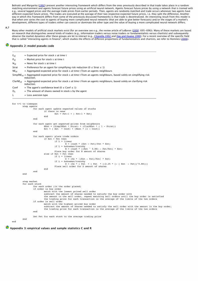
Appendix 2: model pseudo code

Est = Expected price for stock s at time tPst = Market price for stock s at time tNst = News for stock s at time tStrat = Preference for an agent for simplifying risk reduction (0 ≤ Strat ≤ 1)NEst = Aggregated expected price for stock s at time t from an agents neighboursSimplNEst = Aggregated expected price for stock s at time t from an agents neighbours, based solely on simplifying risk

reduction.ClarNEst = Aggregated expected price for stock s at time t from an agents neighbours, based solely on clarifying risk

reduction.Conf = The agent's confidence level (0 ≤ Conf ≤ 1)Os = The amount of shares owned in stock s by the agentL = Loss aversion type

for t=1 to timespan step agents for each agent update expected values of stocks if there is news Est = Pst-1 + ( Pst-1 * Nst) end end

for each agent get expected prices from neighbours NEst = (SimplNEst * Strat) + (ClarNEst * ( 1 - Strat)) Est = ( Est * Conf) + (Nest * (1 - Conf)) end

for each agent: place trade orders if Est > Pst then if L = linear B = (cash * (Est — Pst)/Pst * Est) if L = kahneman/tversky B = (cash * ((Est ^ 0.88) — Pst/Pst) * Est) Place buy order for B amount of shares else if Est < Pst then if L = linear S = (Os * |(Est - Pst)/Pst| * Est) if L = kahneman/tversky S = (Os * ( Pst + ( Pst * (-2.25 * (- ( Est - Pst))^0.88))) Place sell order for S amount of shares end end end

step market for each stock for each order (in the order placed) if order is buy order match with the lowest priced sell order subtract the amount of shares needed to satisfy the buy order with the amount in the sell order, repeat matching sell orders until the buy order is satisfied the trading price for each transaction is the average of the limits of the two orders if order is sell order match with the highest priced buy order subtract the amount of shares needed to satisfy the sell order with the amount in the buy order, repeat matching sell orders until the sell order is satisfied the trading price for each transaction is the average of the limits of the two orders end

Set Pst for each stock to the average trading price end end

Appendix 3: empirical values and sample statistics C and R

Return to Contents of this issue

© Copyright Journal of Artificial Societies and Social Simulation, [2007]