socio-economic causes and … causes and consequences of future environmental changes workshop ......
TRANSCRIPT
SOCIO-ECONOMIC CAUSES AND CONSEQUENCES OF FUTURE ENVIRONMENTAL CHANGES WORKSHOP
A WORKSHOP SPONSORED BY THE U.S. ENVIRONMENTAL PROTECTION AGENCY’S NATIONAL CENTER FOR ENVIRONMENTAL ECONOMICS (NCEE),
NATIONAL CENTER FOR ENVIRONMENTAL RESEARCH (NCER)
November 16, 2005
EPA Region 9 Building
75 Hawthorne Street 1st Floor Conference Room San Francisco, CA
Prepared by Alpha-Gamma Technologies, Inc. 4700 Falls of Neuse Road, Suite 350, Raleigh, NC 27609
ACKNOWLEDGEMENTS
This report has been prepared by Alpha-Gamma Technologies, Inc. with funding from the National Center for Environmental Economics (NCEE). Alpha-Gamma wishes to thank NCEE’s Cynthia Morgan and Jennifer Bowen and the Project Officer, Cheryl R. Brown, for their guidance and assistance throughout this project.
DISCLAIMER
These proceedings are being distributed in the interest of increasing public understanding and knowledge of the issues discussed at the workshop and have been prepared independently of the workshop. Although the proceedings have been funded in part by the United States Environmental Protection Agency under Contract No. 68-W-01-055 to Alpha-Gamma Technologies, Inc., the contents of this document may not necessarily reflect the views of the Agency and no official endorsement should be inferred.
U.S. Environmental Protection Agency Socio-Economic Causes and Consequences of Future Environmental Changes Workshop
November 16, 2005
EPA Region 9 75 Hawthorne Street
1St Floor Conference Room San Francisco, CA
8:45-9:15 Registration
9:15 -9:30 Introductory Remarks – Tom Huetteman, Deputy Assistant Regional Administrator, USEPA Pacific Southwest Region 9
9:30-11:30 Session I: Trends in Housing, Land Use, and Land Cover Change
Session Moderator: Jan Baxter, US EPA, Region 9, Senior Science Policy Advisor
9:30 – 10:00 Determinants of Land Use Conversion on the Southern Cumberland
Plateau Robert Gottfried (presenter), Jonathan Evans, David Haskell, and Douglass Williams, University of the South
10:00– 10:30 Integrating Economic and Physical Data to Forecast Land Use Change and
Environmental Consequences for California’s Coastal Watersheds Kathleen Lohse, David Newburn, and Adina Merenlender (presenter), University of California at Berkeley
10:30 – 10:45 Break 10:45 – 11:00 Discussant: Steve Newbold, US EPA, National Center for
Environmental Economics 11:00 – 11:15 Discussant: Heidi Albers, Oregon State University
11:15 – 11:30 Questions and Discussions
11:30 – 12:30 Lunch
12:30 –2:30 Session II: The Economic and Demographic Drivers of Aquaculture and Greenhouse Gas Emissions Growth
Session Moderator: Bobbye Smith, U.S. EPA Region 9
12:30 – 1:00 Future Growth of the U.S. Aquaculture Industry and Associated Environmental Quality Issues Di Jin (presenter), Porter Hoagland, and Hauke Kite Powell, Woods Hole Oceanographic Institution
1

1:00 – 1:30 Households, Consumption, and Energy Use: The Role of Demographic Change in Future U.S. Greenhouse Gas Emissions
Brian O’Neill, Brown University, Michael Dalton (presenter), California State University – Monterey Bay, John Pitkin, Alexia Prskawetz, Max Planck Institute for Demographic Research
1:30 – 1:45 Discussant: Tim Eichenberg, The Ocean Conservancy 1:45 – 2:00 Discussant: Charles Kolstad, University of California at Santa Barbara
2:00 – 2:30 Questions and Discussion
2:30 – 2:45 Break 2:45 - 4:55 Session III: New Research: Land Use, Transportation, and Air Quality
Session Moderator: Kathleen Dadey, US EPA, Region 9, Co-chair of the Regional Science Council
2:45 - 3:10 Transforming Office Parks Into Transit Villages: Pleasanton's
Hacienda Business Park Steve Raney (presenter), Cities21
3:10 – 3:35 Methodology for Assessing the Effects of Technological and Economic
Changes on the Location, Timing and Ambient Air Quality Impacts of Power Sector Emissions Joseph Ellis and Benjamin Hobbs (presenter), Johns Hopkins University, Dallas Burtaw and Karen Palmer, Resources for the Future
3:35 - 4:00 Integrating Land Use, Transportation and Air Quality Modeling
Paul Waddell (presenter), University of Washington
4:00- 4:25 Regional Development, Population Trend, and Technology Change Impacts on Future Air Pollution Emissions in the San Joaquin Valley
Michael Kleeman, Deb Niemeier, Susan Handy (presenter), Jay Lund, Song Bai, Sangho Choo, Julie Ogilvie, Shengyi Gao, University of California at Davis
4:25 – 4:55 Questions and Discussion 4:55 – 5:00 Wrap-Up and Closing Comments
2
[email protected], slide 1
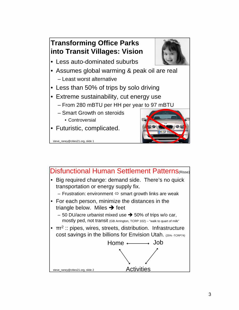
Transforming Office Parks into Transit Villages: Vision• Less auto-dominated suburbs• Assumes global warming & peak oil are real
– Least worst alternative• Less than 50% of trips by solo driving• Extreme sustainability, cut energy use
– From 280 mBTU per HH per year to 97 mBTU– Smart Growth on steroids
• Controversial
• Futuristic, complicated.
[email protected], slide 2
Disfunctional Human Settlement Patterns(Risse)
• Big required change: demand side. There’s no quick transportation or energy supply fix.– Frustration: environment smart growth links are weak
• For each person, minimize the distances in the triangle below. Miles feet– 50 DU/acre urbanist mixed use 50% of trips w/o car,
mostly ped, not transit (GB Arrington, TCRP 102) – “walk to quart of milk”
• πr2 :: pipes, wires, streets, distribution. Infrastructure cost savings in the billions for Envision Utah. (25% -TCRP74)
Home Job
Activities
3
[email protected], slide 3
The Villain: Suburban Office Parks• Main cause of sprawl & congestion for 30 years
– Affordability decreasing, segregation increasing– 200 with ~ 30K workers 6M+ workers
• ULI’s Transforming Suburban Business Districts• Calthorpe "We didn't focus on office parks. Huge
mistake. Need powerful strategies for these”• Cervero: So bad they’re easy to fix• Shoup (High Cost of Free Parking) - Parking lots land
bank. The new frontier: 5 spaces per car• Duany: "Upper Rock" business park TOD• Rail~Volution session: Tyson’s edgy TOD• 70% of tech workers want urban vitality.
[email protected], slide 4
Villain 2: Housing Industry• Problem: few innovative housing choices • 1) Zimmerman / Volk. Home industry: "lumbering
giants.” No genuine innovations. No “meaningful improvement of the product offered to the consumer"
• 2) SG America: "Homes are like pork bellies, all the same, rather than as consumer products which vary greatly according to people's preferences.” HPD #12i4
• New choice: vibrant, green suburban lifestyle: short commute apts and condos, mixed use, good schools.
(By John S. Pritchett
www.pritchettcartoons.com)
4
[email protected], slide 5
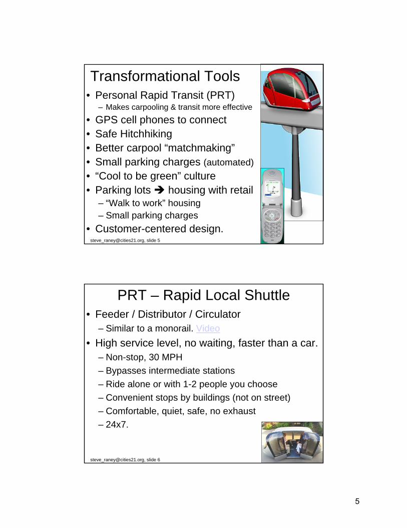
Transformational Tools• Personal Rapid Transit (PRT)
– Makes carpooling & transit more effective
• GPS cell phones to connect• Safe Hitchhiking• Better carpool “matchmaking”• Small parking charges (automated)• “Cool to be green” culture• Parking lots housing with retail
– “Walk to work” housing– Small parking charges
• Customer-centered design.
[email protected], slide 6
PRT – Rapid Local Shuttle• Feeder / Distributor / Circulator
– Similar to a monorail. Video• High service level, no waiting, faster than a car.
– Non-stop, 30 MPH– Bypasses intermediate stations– Ride alone or with 1-2 people you choose– Convenient stops by buildings (not on street)– Comfortable, quiet, safe, no exhaust– 24x7.
5
[email protected], slide 7
[email protected], slide 8
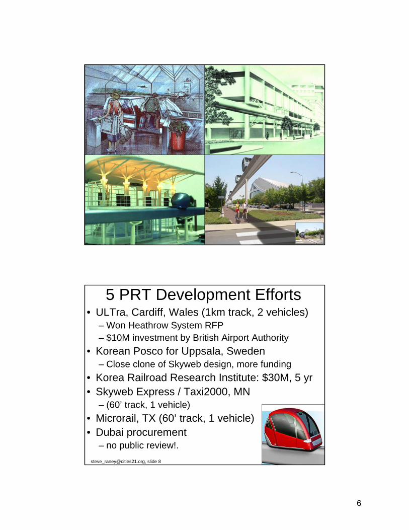
5 PRT Development Efforts• ULTra, Cardiff, Wales (1km track, 2 vehicles)
– Won Heathrow System RFP– $10M investment by British Airport Authority
• Korean Posco for Uppsala, Sweden– Close clone of Skyweb design, more funding
• Korea Railroad Research Institute: $30M, 5 yr• Skyweb Express / Taxi2000, MN
– (60’ track, 1 vehicle)• Microrail, TX (60’ track, 1 vehicle)• Dubai procurement
– no public review!.
6
[email protected], slide 9
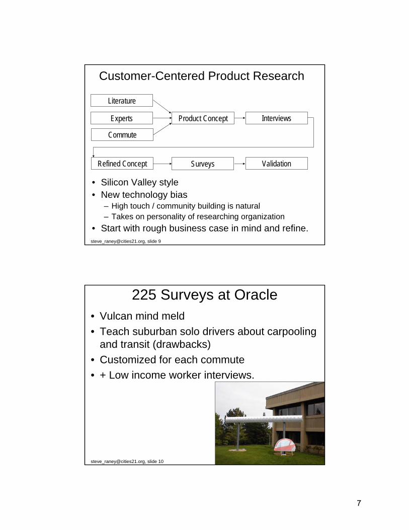
Customer-Centered Product Research
Literature
Product Concept InterviewsExperts
Commute
Refined Concept Surveys Validation
• Silicon Valley style • New technology bias
– High touch / community building is natural– Takes on personality of researching organization
• Start with rough business case in mind and refine.
[email protected], slide 10
225 Surveys at Oracle• Vulcan mind meld• Teach suburban solo drivers about carpooling
and transit (drawbacks)• Customized for each commute• + Low income worker interviews.
7
[email protected], slide 11
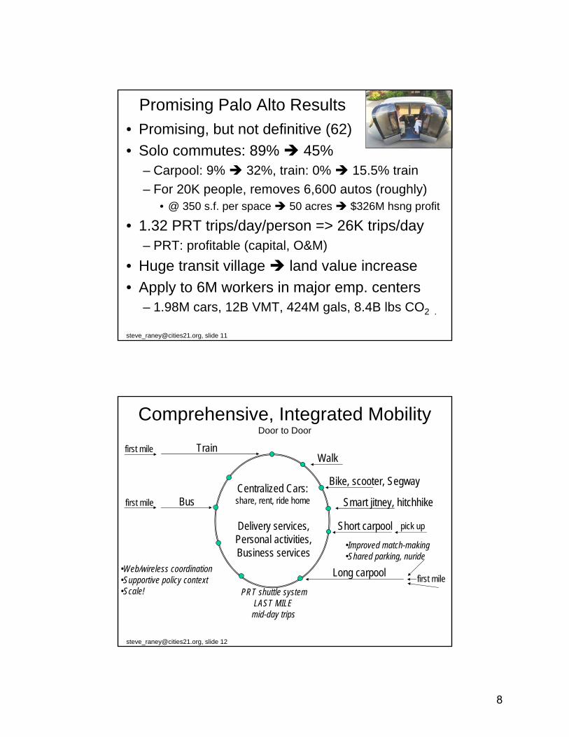
Promising Palo Alto Results• Promising, but not definitive (62)• Solo commutes: 89% 45%
– Carpool: 9% 32%, train: 0% 15.5% train– For 20K people, removes 6,600 autos (roughly)
• @ 350 s.f. per space 50 acres $326M hsng profit
• 1.32 PRT trips/day/person => 26K trips/day– PRT: profitable (capital, O&M)
• Huge transit village land value increase• Apply to 6M workers in major emp. centers
– 1.98M cars, 12B VMT, 424M gals, 8.4B lbs CO2 .
[email protected], slide 12
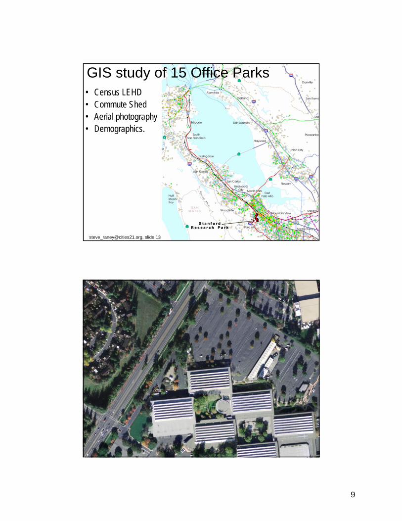
Comprehensive, Integrated MobilityDoor to Door
Centralized Cars:share, rent, ride home
Delivery services, Personal activities, Business services
first mile Train
first mile Bus
Walk
Bike, scooter, Segway
Smart jitney, hitchhike
•Web/wireless coordination•Supportive policy context•Scale!
Short carpool pick up
first mileLong carpool
•Improved match-making•Shared parking, nuride
PRT shuttle systemLAST MILEmid-day trips
8
[email protected], slide 13
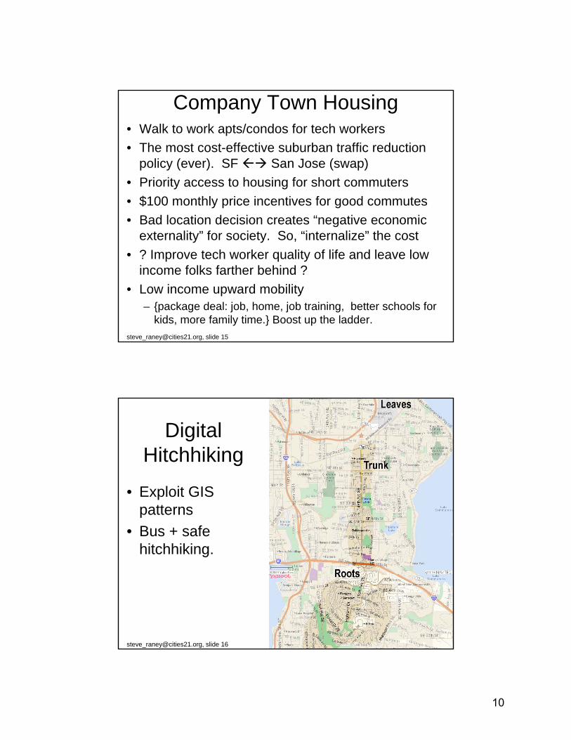
GIS study of 15 Office Parks • Census LEHD• Commute Shed• Aerial photography• Demographics.
[email protected], slide 14
9
[email protected], slide 15
Company Town Housing• Walk to work apts/condos for tech workers• The most cost-effective suburban traffic reduction
policy (ever). SF San Jose (swap)• Priority access to housing for short commuters• $100 monthly price incentives for good commutes• Bad location decision creates “negative economic
externality” for society. So, “internalize” the cost• ? Improve tech worker quality of life and leave low
income folks farther behind ?• Low income upward mobility
– {package deal: job, home, job training, better schools for kids, more family time.} Boost up the ladder.
[email protected], slide 16
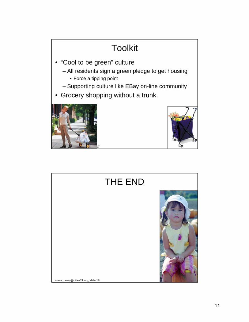
Digital Hitchhiking
• Exploit GIS patterns
• Bus + safe hitchhiking.
10
[email protected], slide 17
Toolkit• “Cool to be green” culture
– All residents sign a green pledge to get housing• Force a tipping point
– Supporting culture like EBay on-line community• Grocery shopping without a trunk.
[email protected], slide 18
THE END
11
Assessing the Effects of Technological & Economic Changes on the
Location, Timing, and Ambient Air Quality Impacts of Power Sector Emissions
InvestigatorsHugh Ellis (PI), Ben HobbsThe Johns Hopkins University
Dallas Burtraw, Karen PalmerResources for the Future
R831836
Develop methodology for:– creating geographically and temporally disaggregated emissions
scenarios– for the electric power sector – on a multidecadal time-scale
• Source of a large share of SOx, NOx, mercury and CO2 emissions– Future shares are highly uncertain– Technology change, fuel mix, electric load growth, regulation
• Alternative scenarios affect total emissions and their spatial and temporal distribution
• Emissions & air quality impacts sensitive to the growth and distribution of electricity demands – Geographically and temporally – Linked to temperature and other climate variables that may change
significantly
PURPOSE
WHY POWER?
12
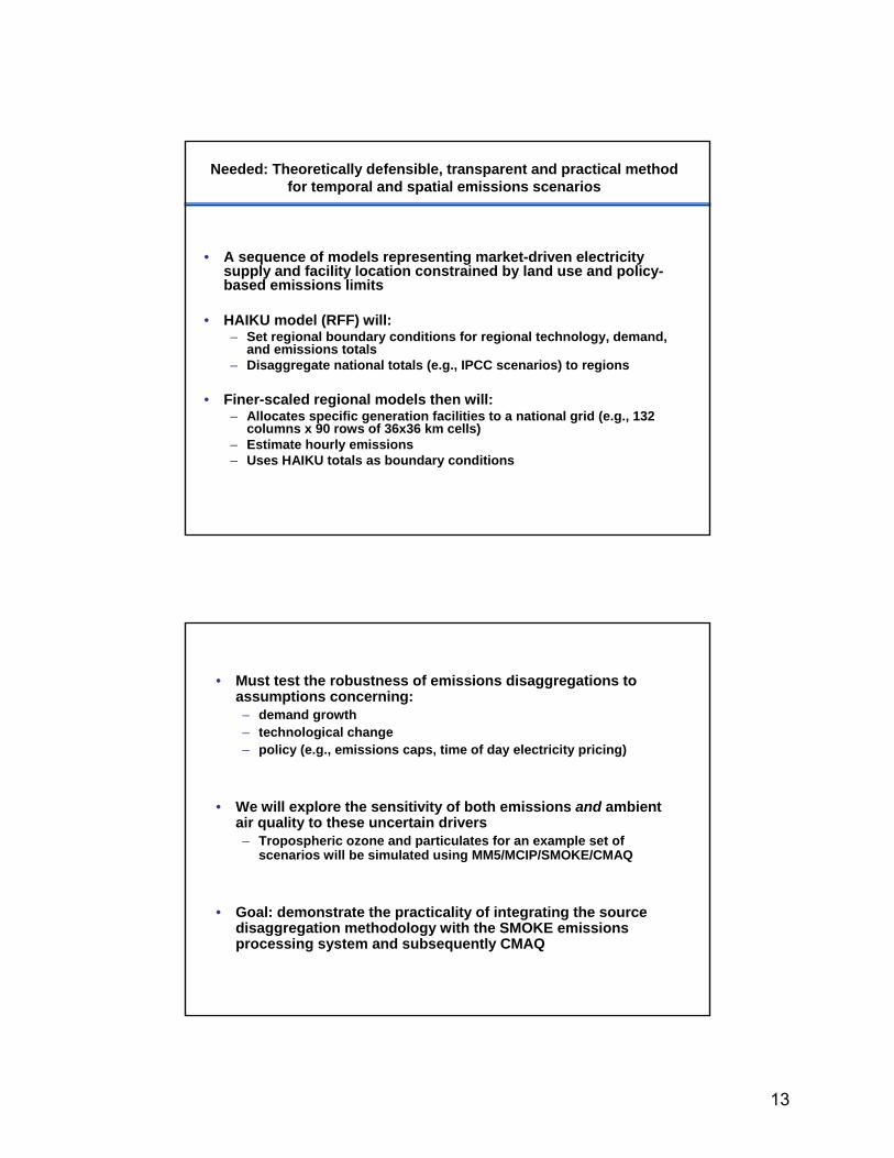
Needed: Theoretically defensible, transparent and practical method for temporal and spatial emissions scenarios
• A sequence of models representing market-driven electricity supply and facility location constrained by land use and policy-based emissions limits
• HAIKU model (RFF) will:– Set regional boundary conditions for regional technology, demand,
and emissions totals– Disaggregate national totals (e.g., IPCC scenarios) to regions
• Finer-scaled regional models then will: – Allocates specific generation facilities to a national grid (e.g., 132
columns x 90 rows of 36x36 km cells)– Estimate hourly emissions– Uses HAIKU totals as boundary conditions
• Must test the robustness of emissions disaggregations to assumptions concerning:– demand growth – technological change – policy (e.g., emissions caps, time of day electricity pricing)
• We will explore the sensitivity of both emissions and ambient air quality to these uncertain drivers – Tropospheric ozone and particulates for an example set of
scenarios will be simulated using MM5/MCIP/SMOKE/CMAQ
• Goal: demonstrate the practicality of integrating the source disaggregation methodology with the SMOKE emissions processing system and subsequently CMAQ
13
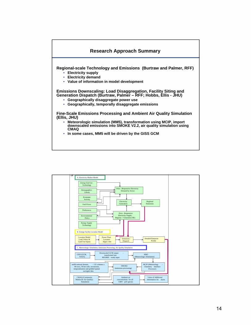
Research Approach Summary
Regional-scale Technology and Emissions (Burtraw and Palmer, RFF)• Electricity supply • Electricity demand• Value of information in model development
Emissions Downscaling: Load Disaggregation, Facility Siting and Generation Dispatch (Burtraw, Palmer – RFF; Hobbs, Ellis - JHU)
• Geographically disaggregate power use• Geographically, temporally disaggregate emissions
Fine-Scale Emissions Processing and Ambient Air Quality Simulation (Ellis, JHU)
• Meteorologic simulation (MM5), transformation using MCIP, import downscaled emissions into SMOKE V2.2, air quality simulation using CMAQ
• In some cases, MM5 will be driven by the GISS GCM
Energy End UseTechnology
DemographicsLibrary
Economic Activity
Fuel Prices
Preferences
Environmental Policy
ElectricityGeneration
Regional Emissions
Energy SupplyTechnology
A. Electricity Market Model
B. Energy Facility Location Model
C. Meteorologic Simulation, Emissions Processing, Air Quality Simulation
Location Model Load, Policy &
Land Use Inputs
Power PlantLocation
Algori thm
Detailed EmissionProfile
MM5 (Meteorologic Simulation)
GISS (GCM, NASA)
SMOKE (emissions processing)
Downscaled GCM output –transformed into
REGRID -ready input
CMAQ (Community Mutliscale Air Quality)
Simulation
MCIP (Meteorology –Chemistry Interface
Processor)
Ambient air concentrations for all
CBIV -p25 species
net96 national domain – 132 columns x 90 rows, 36 km cells; inventories,
temporalization and gridded spatial surrogate data
Price -Responsive Electricity Demand by Sector
Price -Responsive Electricity Supply,
Regiona l Generation Mix
EmissionsDispatch
Value of Additional Information An alysis
14
Energy End UseTechnology
DemographicsLibrary
Economic Activity
Fuel Prices
Preferences
Environmental Policy
ElectricityGeneration
Regional Emissions
Energy SupplyTechnology
A. Electricity Market Model
B. Energy Facility Location Model
C. Meteorologic Simulation, Emissions Processing, Air Quality Simulation
Location Model Load, Policy &
Land Use Inputs
Power PlantLocation
Algori thm
Detailed EmissionProfile
MM5 (Meteorologic Simulation)
GISS (GCM, NASA)
SMOKE (emissions processing)
Downscaled GCM output –transformed into
REGRID -ready input
CMAQ (Community Mutliscale Air Quality)
Simulation
MCIP (Meteorology –Chemistry Interface
Processor)
Ambient air concentrations for all
CBIV -p25 species
net96 national domain – 132 columns x 90 rows, 36 km cells; inventories,
temporalization and gridded spatial surrogate data
Price -Responsive Electricity Demand by Sector
Price -Responsive Electricity Supply,
Regiona l Generation Mix
EmissionsDispatch
Value of Additional Information An alysis
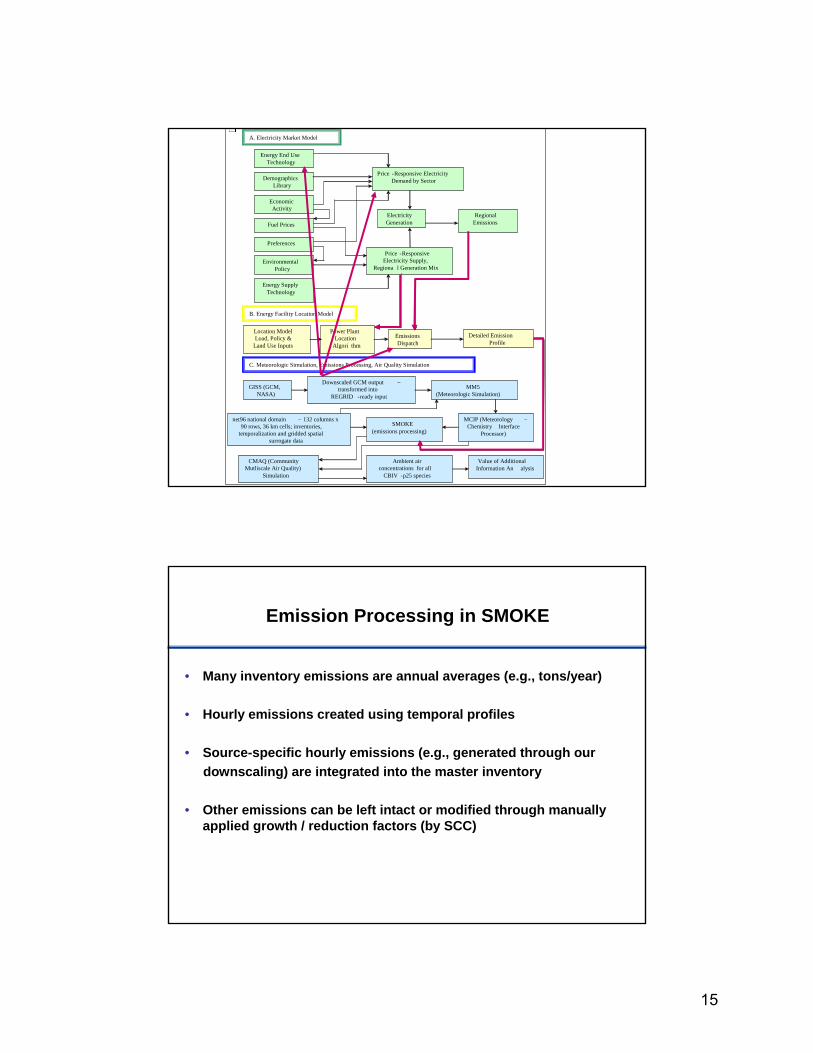
Emission Processing in SMOKE
• Many inventory emissions are annual averages (e.g., tons/year)
• Hourly emissions created using temporal profiles
• Source-specific hourly emissions (e.g., generated through ourdownscaling) are integrated into the master inventory
• Other emissions can be left intact or modified through manually applied growth / reduction factors (by SCC)
15
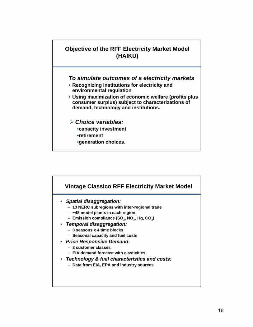
Objective of the RFF Electricity Market Model (HAIKU)
To simulate outcomes of a electricity markets • Recognizing institutions for electricity and
environmental regulation • Using maximization of economic welfare (profits plus
consumer surplus) subject to characterizations of demand, technology and institutions.
Choice variables:•capacity investment•retirement•generation choices.
Vintage Classico RFF Electricity Market Model
• Spatial disaggregation:– 13 NERC subregions with inter-regional trade– ~48 model plants in each region– Emission compliance (SO2, NOX, Hg, CO2)
• Temporal disaggregation:– 3 seasons x 4 time blocks– Seasonal capacity and fuel costs
• Price Responsive Demand: – 3 customer classes – EIA demand forecast with elasticities
• Technology & fuel characteristics and costs:– Data from EIA, EPA and industry sources
16
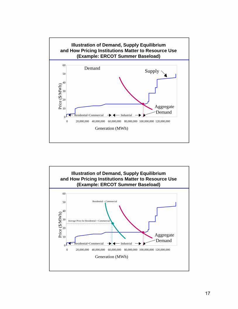
Illustration of Demand, Supply Equilibriumand How Pricing Institutions Matter to Resource Use
(Example: ERCOT Summer Baseload)
0
10
20
30
40
50
60
0 20,000,000 40,000,000 60,000,000 80,000,000 100,000,000 120,000,000
Generation (MWh)
Pric
e ($
/MW
h)
Supply
Residential+Commercial Industrial
AggregateDemand
Demand
Illustration of Demand, Supply Equilibriumand How Pricing Institutions Matter to Resource Use
(Example: ERCOT Summer Baseload)
0
10
20
30
40
50
60
0 20,000,000 40,000,000 60,000,000 80,000,000 100,000,000 120,000,000
Generation (MWh)
Pric
e ($
/MW
h)
Residential+Commercial Industrial
AggregateDemand
Average Price for Residential + Commercial
Residential + Commercial
17
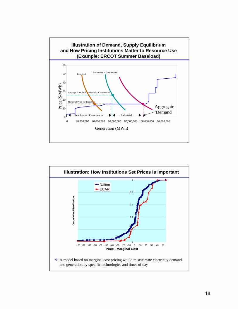
Illustration of Demand, Supply Equilibriumand How Pricing Institutions Matter to Resource Use
(Example: ERCOT Summer Baseload)
0
10
20
30
40
50
60
0 20,000,000 40,000,000 60,000,000 80,000,000 100,000,000 120,000,000
Generation (MWh)
Pric
e ($
/MW
h)
Residential+Commercial Industrial
AggregateDemand
Average Price for Residential + Commercial
Marginal Price for Industrial
Residential + CommercialIndustrial
Illustration: How Institutions Set Prices Is Important
0
0.2
0.4
0.6
0.8
1
-100 -90 -80 -70 -60 -50 -40 -30 -20 -10 0 10 20 30 40 50
Price - Marginal Cost
Cum
ulat
ive
Dis
trib
utio
n
NationECAR
A model based on marginal cost pricing would misestimate electricity demand and generation by specific technologies and times of day
18
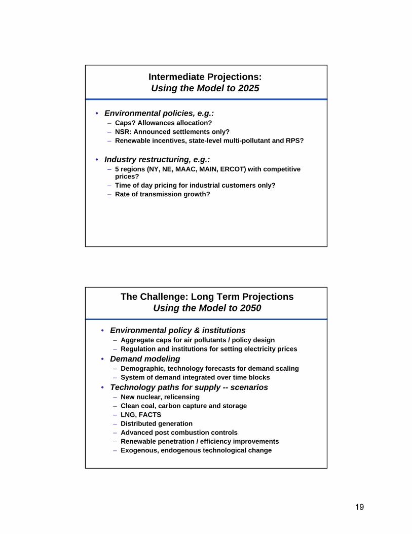
Intermediate Projections:Using the Model to 2025
• Environmental policies, e.g.:– Caps? Allowances allocation?– NSR: Announced settlements only?– Renewable incentives, state-level multi-pollutant and RPS?
• Industry restructuring, e.g.: – 5 regions (NY, NE, MAAC, MAIN, ERCOT) with competitive
prices? – Time of day pricing for industrial customers only?– Rate of transmission growth?
• Environmental policy & institutions– Aggregate caps for air pollutants / policy design– Regulation and institutions for setting electricity prices
• Demand modeling– Demographic, technology forecasts for demand scaling– System of demand integrated over time blocks
• Technology paths for supply -- scenarios– New nuclear, relicensing– Clean coal, carbon capture and storage– LNG, FACTS– Distributed generation– Advanced post combustion controls– Renewable penetration / efficiency improvements– Exogenous, endogenous technological change
The Challenge: Long Term ProjectionsUsing the Model to 2050
19
Recent Applications of the HAIKU Model
• “Cost-Effectiveness of Renewable Electricity Policies,” (Palmer and Burtraw) 2006. Energy Economics, forthcoming.
• Reducing Emissions from the Electricity Sector: The Costs and Benefits Nationwide and in the Empire State, (Palmer, Burtraw and Shih) 2005. New York State Energy Research and Development Authority, Report 05-02.
• “Efficient Emission Fees in the U.S. Electricity Sector,” (Banzhaf, Burtraw and Palmer) 2004. Resource and Energy Economics 26(3): 317-341.
• “Uncertainty and the Net Benefits of NOX Emissions Reductions from Electricity Generation,” (Burtraw, Bharvirkar and McGuinness) 2003. Land Economics79(3): 382-401.
• “Ancillary Benefits of Reduced Air Pollution in the United States from Moderate Greenhouse Gas Mitigation Policies in the Electricity Sector,” (Burtraw, Krupnick, Palmer, Paul, Toman and Bloyd) 2003. Journal of Environmental Economics and Management 45(3): 650-673.
• Economic Efficiency and Distributional Consequences of Different Approaches to NOx and SO2 Allowance Allocation, Burtraw and Palmer, Oct. 2003. Report to U.S. EPA.
• “The Effect on Asset Values of the Allocation of Carbon Dioxide Emission Allowances,” (with Karen Palmer, Anthony Paul and Ranjit Bharvirkar) 2002. The Electricity Journal 15 (5): 51-62.
The Downscaling Problem
• National electric sector models are aggregate in space and time. RFF model:– 13 NERC subregions– 12 time blocks per year– Based on average seasonal climate conditions
• The challenges:– CMAQ requires hourly emissions by point source– CMAQ results sensitive to interactions of location,
meteorology and timing– There is significant interannual variation in climate
and, thus, emissions and their impacts
20
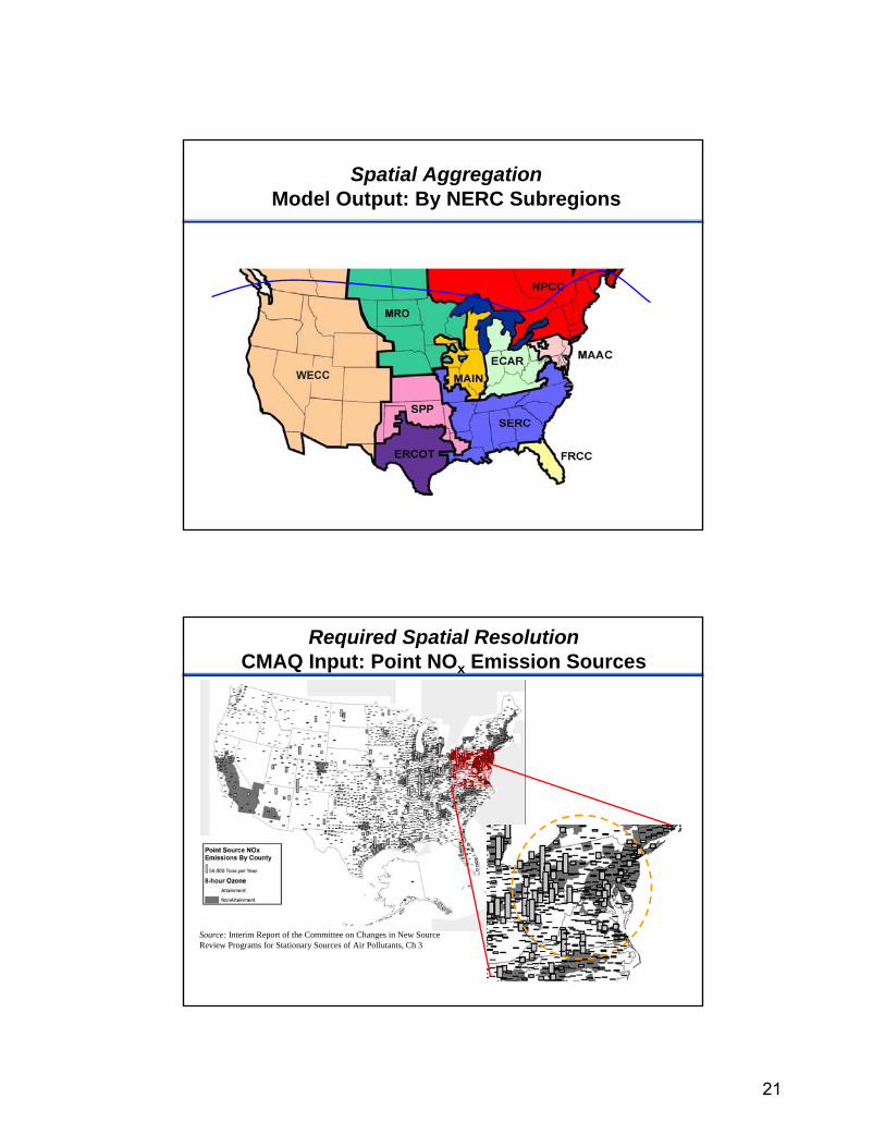
Spatial AggregationModel Output: By NERC Subregions
Required Spatial Resolution CMAQ Input: Point NOx Emission Sources
Source: Interim Report of the Committee on Changes in New Source Review Programs for Stationary Sources of Air Pollutants, Ch 3
21
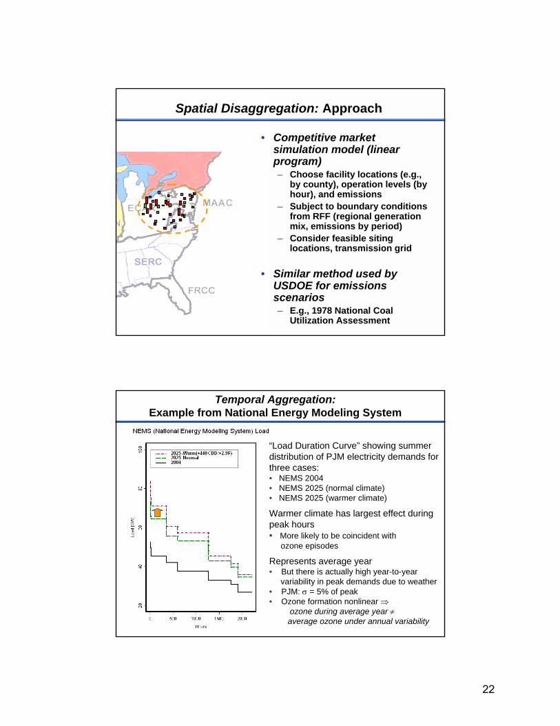
• Competitive market simulation model (linear program)– Choose facility locations (e.g.,
by county), operation levels (by hour), and emissions
– Subject to boundary conditions from RFF (regional generation mix, emissions by period)
– Consider feasible siting locations, transmission grid
• Similar method used by USDOE for emissions scenarios– E.g., 1978 National Coal
Utilization Assessment
Spatial Disaggregation: Approach
Temporal Aggregation:Example from National Energy Modeling System
“Load Duration Curve” showing summer distribution of PJM electricity demands for three cases:• NEMS 2004• NEMS 2025 (normal climate)• NEMS 2025 (warmer climate)
Warmer climate has largest effect during peak hours• More likely to be coincident with
ozone episodes
Represents average year• But there is actually high year-to-year
variability in peak demands due to weather• PJM: σ = 5% of peak• Ozone formation nonlinear ⇒
ozone during average year ≠average ozone under annual variability
22
NEMS (National Energy Modeling System) Load
Hours
Load
[GW
]
0 500 1000 1500 2000
2040
6080
100
2025-Warm(+440CDD/+2.9F)2025-Normal2004
Average Load Duration Curves
Hours
Load
[GW
]
0 1000 2000 3000
2040
6080
100
2050s Climate1990s Climate
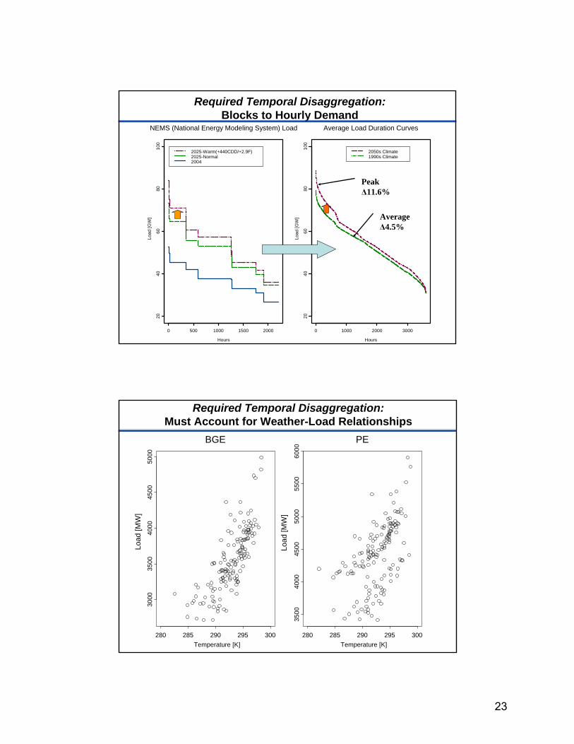
Peak∆11.6%
Average∆4.5%
Required Temporal Disaggregation:Blocks to Hourly Demand
Required Temporal Disaggregation:Must Account for Weather-Load Relationships
BGE
Temperature [K]280 285 290 295 300
3000
3500
4000
4500
5000
PE
Temperature [K]280 285 290 295 300
3500
4000
4500
5000
5500
6000
Load
[MW
]
Load
[MW
]
23
Hours
Load
[GW
]
0 1000 2000 3000
2040
6080
100
2055205119981994
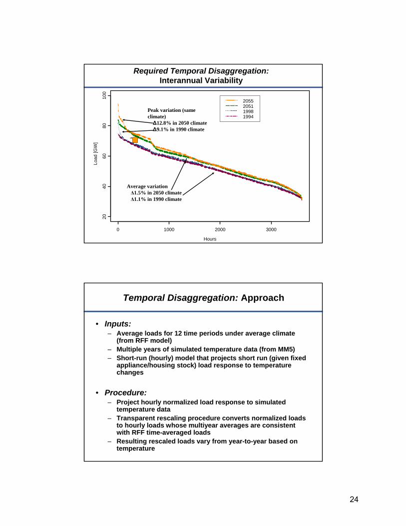
Required Temporal Disaggregation:Interannual Variability
Peak variation (same climate) ∆12.8% in 2050 climate∆9.1% in 1990 climate
Average variation∆1.5% in 2050 climate∆1.1% in 1990 climate
• Inputs: – Average loads for 12 time periods under average climate
(from RFF model)– Multiple years of simulated temperature data (from MM5)– Short-run (hourly) model that projects short run (given fixed
appliance/housing stock) load response to temperature changes
• Procedure:– Project hourly normalized load response to simulated
temperature data– Transparent rescaling procedure converts normalized loads
to hourly loads whose multiyear averages are consistent with RFF time-averaged loads
– Resulting rescaled loads vary from year-to-year based on temperature
Temporal Disaggregation: Approach
24
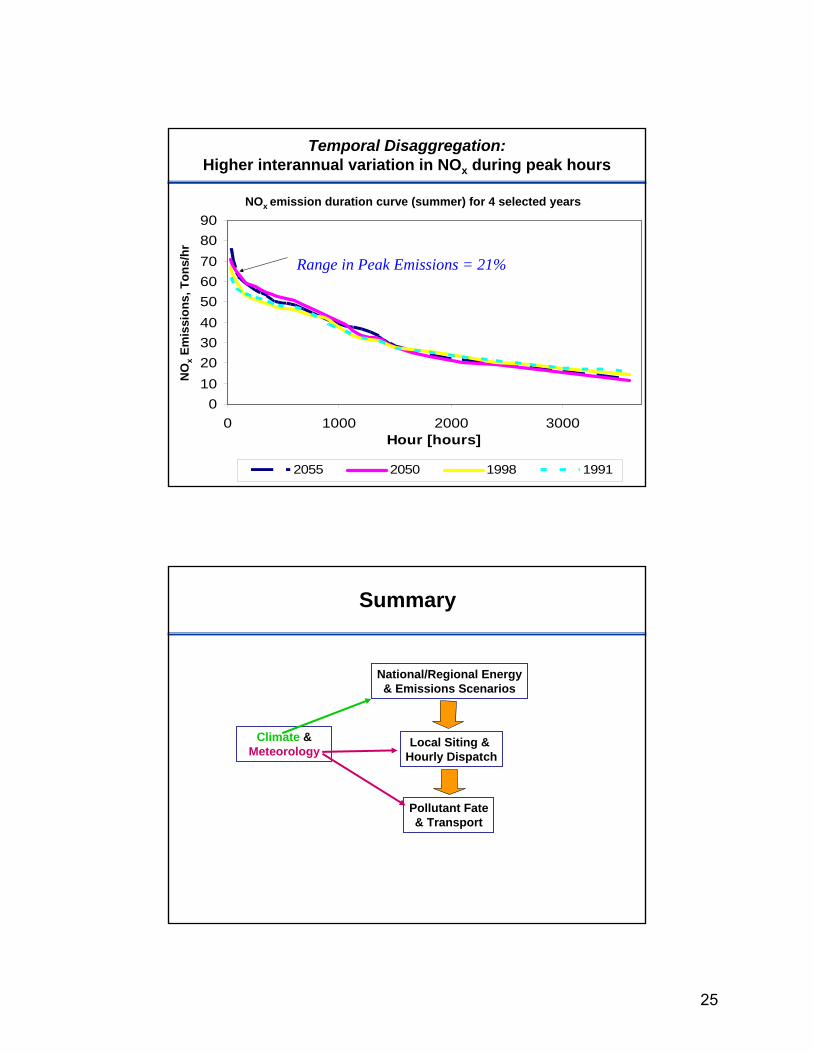
NOx emission duration curve (summer) for 4 selected years
0102030405060708090
0 1000 2000 3000Hour [hours]
NO
x em
issi
on [t
on/h
our]
2055 2050 1998 1991
Temporal Disaggregation: Higher interannual variation in NOx during peak hours
Range in Peak Emissions = 21%
NO
xEm
issi
ons,
Ton
s/hr
NOx emission duration curve (summer) for 4 selected years
Summary
National/Regional Energy& Emissions Scenarios
Local Siting & Hourly Dispatch
Pollutant Fate& Transport
Climate &Meteorology
25
Integrating Land Use, Transportation and Integrating Land Use, Transportation and Air Quality ModelingAir Quality Modeling
SocioSocio--Economic Causes and Consequences of Economic Causes and Consequences of Future Environmental Changes WorkshopFuture Environmental Changes Workshop
November 16, 2005November 16, 2005
Paul [email protected]
Center for Urban Simulation and Policy AnalysisEvans School of Public Affairs
University of Washingtonhttp://www.urbansim.org
AgendaAgenda
Research AgendaEPA STAR ProjectUrbanSimA Brief Example
26

Center for Urban Simulation and Policy AnalysisCenter for Urban Simulation and Policy AnalysisUniversity of WashingtonUniversity of Washington
Core FacultyPaul Waddell, Director, Public Affairs, PlanningAlan Borning, Co-Director, Computer Science and Eng.Marina Alberti, Urban Design and PlanningBatya Friedman, Information SchoolMark Handcock, StatisticsScott Rutherford, Civil and Environmental Engineering
Current (Active) Research ProjectsCurrent (Active) Research Projects
Integrating Land Use, Activity-Based Travel and Air Quality Models (EPA)Integrating Urban Development, Land Cover Change, and Urban Ecology (NSF Biocomplexity)Measuring and Representing Uncertainty in Policy Modeling (NSF Digital Government)Analyzing Distributional Effects of Policies (FHWA Eisenhower Fellowship)Modeling and Measuring Walking and Transit Accessibility (FHWA Eisenhower Fellowship)A Stakeholder Interface for Urban Simulation Models (NSF ITR)Open Platform for Urban Simulation (NSF ITR)Application of UrbanSim to the Puget Sound Region (Puget Sound Regional Council)
27
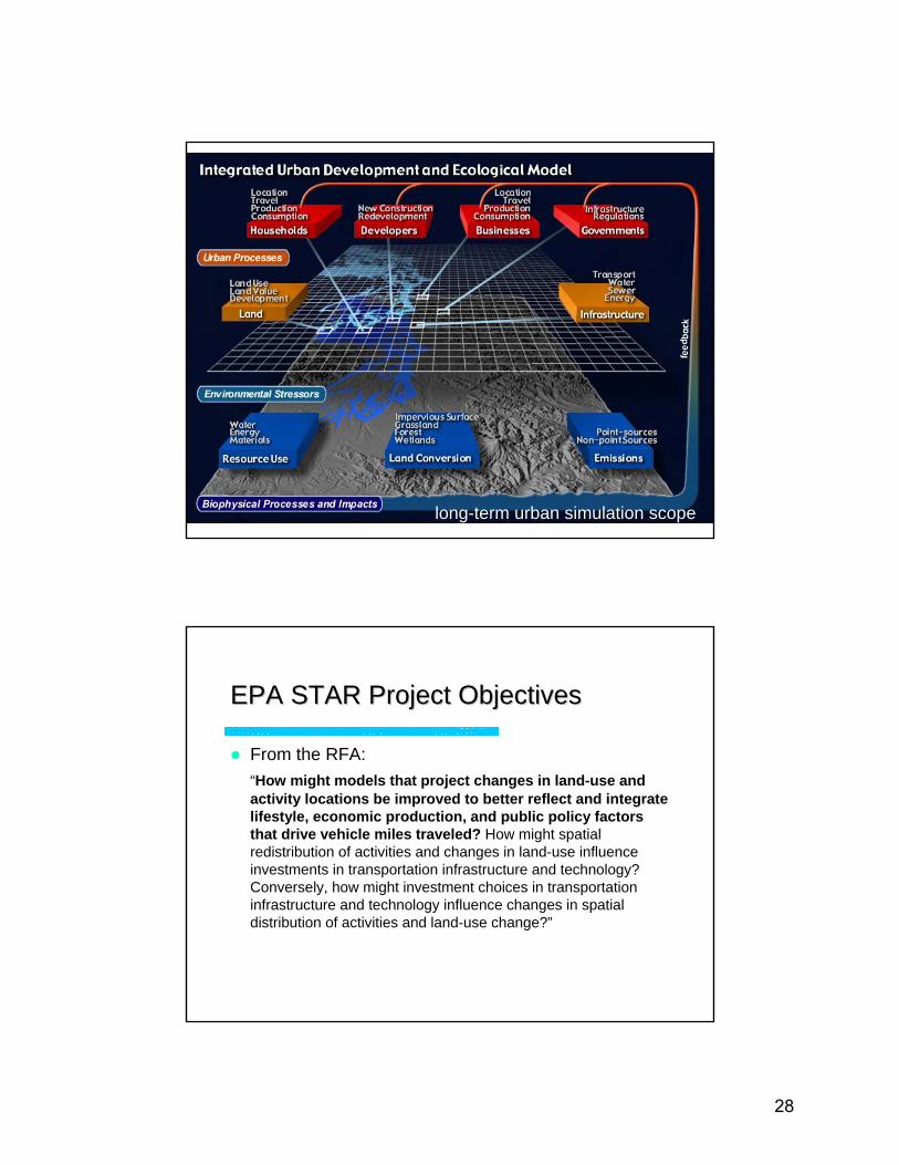
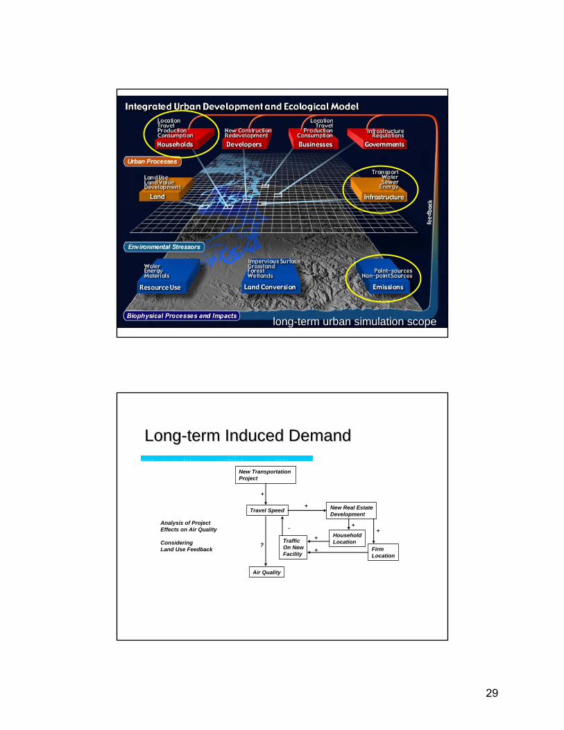
long-term urban simulation scope
EPA STAR Project ObjectivesEPA STAR Project Objectives
From the RFA:“How might models that project changes in land-use and activity locations be improved to better reflect and integrate lifestyle, economic production, and public policy factors that drive vehicle miles traveled? How might spatial redistribution of activities and changes in land-use influence investments in transportation infrastructure and technology? Conversely, how might investment choices in transportation infrastructure and technology influence changes in spatial distribution of activities and land-use change?”
28
long-term urban simulation scope
LongLong--term Induced Demandterm Induced Demand
New Transportation Project
New Real EstateDevelopmentTravel Speed
+
+
HouseholdLocation
FirmLocation
++
TrafficOn NewFacility
+
+
-
Air Quality
?
Analysis of ProjectEffects on Air Quality
ConsideringLand Use Feedback
29
Behavioral and Operational ComponentsBehavioral and Operational Components
Behavioral– Latent lifestyle choices– Substitution across long and short-term choices– Endogeneity and self-selection issues– Econometric estimation methods
Operational– Integration of activity-based models with urban simulation
models of land use– Integration with traffic assignment models– Integration with current and emerging emissions models– Testing of integrated platform on alternative scenarios
Key Operational ComponentsKey Operational Components
UrbanSim/OPUS – urban simulationPCATS/DEBNetS – activity-based travelEPA Moves – emmissions
30
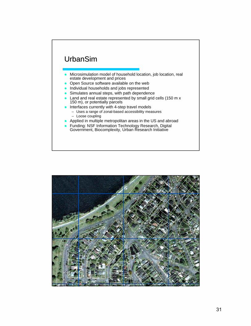
UrbanSimUrbanSim
Microsimulation model of household location, job location, real estate development and pricesOpen Source software available on the webIndividual households and jobs representedSimulates annual steps, with path dependenceLand and real estate represented by small grid cells (150 m x 150 m), or potentially parcelsInterfaces currently with 4-step travel models– Uses a range of zonal-based accessibility measures– Loose coupling
Applied in multiple metropolitan areas in the US and abroadFunding: NSF Information Technology Research, Digital Government, Biocomplexity, Urban Research Initiative
31
Residential Location VariablesResidential Location Variables
Housing Characteristics– Prices (interacted with income)– Development types (density, land use mix)– Housing age
Regional accessibility– Job accessibility by auto-ownership group– Travel time to CBD and airport
Urban design-scale (local accessibility)– Neighborhood land use mix and density– Neighborhood employment– Compensates for large traffic zones in Travel Model
Land Price VariablesLand Price Variables
Site characteristics– Development type– Land use plan– Environmental constraints
Regional accessibility– Access to population and employment
Urban design-scale– Land use mix and density– Proximity to highways and arterials
32
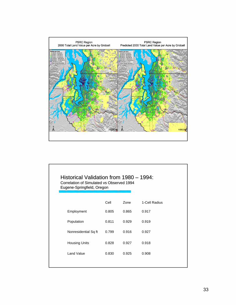
Historical Validation from 1980 Historical Validation from 1980 –– 1994:1994:Correlation of Simulated Correlation of Simulated vsvs Observed 1994Observed 1994EugeneEugene--Springfield, OregonSpringfield, Oregon
0.9080.9250.830Land Value
0.9180.9270.828Housing Units
0.9270.9160.799Nonresidential Sq ft
0.9190.9290.811Population
0.9170.8650.805Employment
1-Cell RadiusZoneCell
33
Creating Policy ScenariosCreating Policy ScenariosMacroeconomic Assumptions– Household and employment control totals
Development constraints– Can select any combination of
• Political and planning overlays• Environmental overlays• Land use plan designation
– Constraints determine which development types cannot be built
Transportation infrastructureUser-specified events
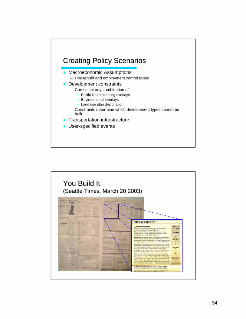
You Build It You Build It (Seattle Times, March 20 2003)(Seattle Times, March 20 2003)
34
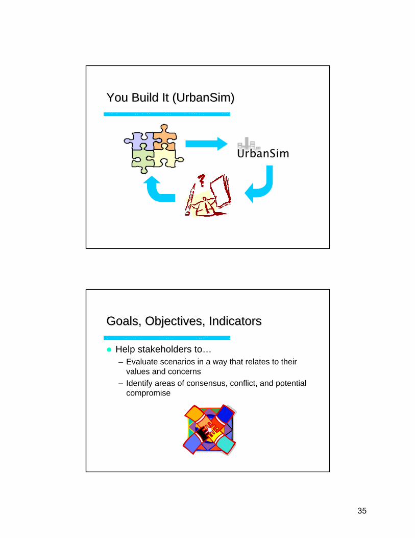
You Build It (UrbanSim)You Build It (UrbanSim)
Assemble Simulate
Evaluate
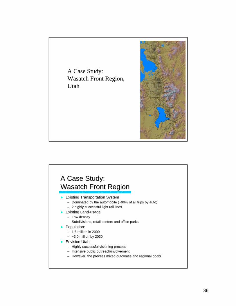
Goals, Objectives, IndicatorsGoals, Objectives, Indicators
Help stakeholders to…– Evaluate scenarios in a way that relates to their
values and concerns– Identify areas of consensus, conflict, and potential
compromise
35
A Case Study:Wasatch Front Region, Utah
A Case Study: A Case Study: Wasatch Front RegionWasatch Front Region
Existing Transportation System– Dominated by the automobile (~90% of all trips by auto)– 2 highly successful light rail lines
Existing Land-usage– Low density– Subdivisions, retail centers and office parks
Population:– 1.6 million in 2000– ~3.0 million by 2030
Envision Utah– Highly successful visioning process– Intensive public outreach/involvement– However, the process mixed outcomes and regional goals
36
Current Modeling Practice at WFRCCurrent Modeling Practice at WFRC
Federally mandated processTransportation Analyses:– Long-range plans (>20 years)– Short-range plans (3-5 years)– Corridor studies
Accepted practice transportation modelsLand-use forecast is independent of planned transportation system
Environmental ConcernsEnvironmental Concerns
Inadequate modeling:– Treatment of land-use (secondary impacts)– Modeling of non-automobile travel– Over-exaggerating congestion in “no-build” or transit
alternativesInadequate planning:– Resource usage– Environmental quality– Sustainability
General Skepticism
37
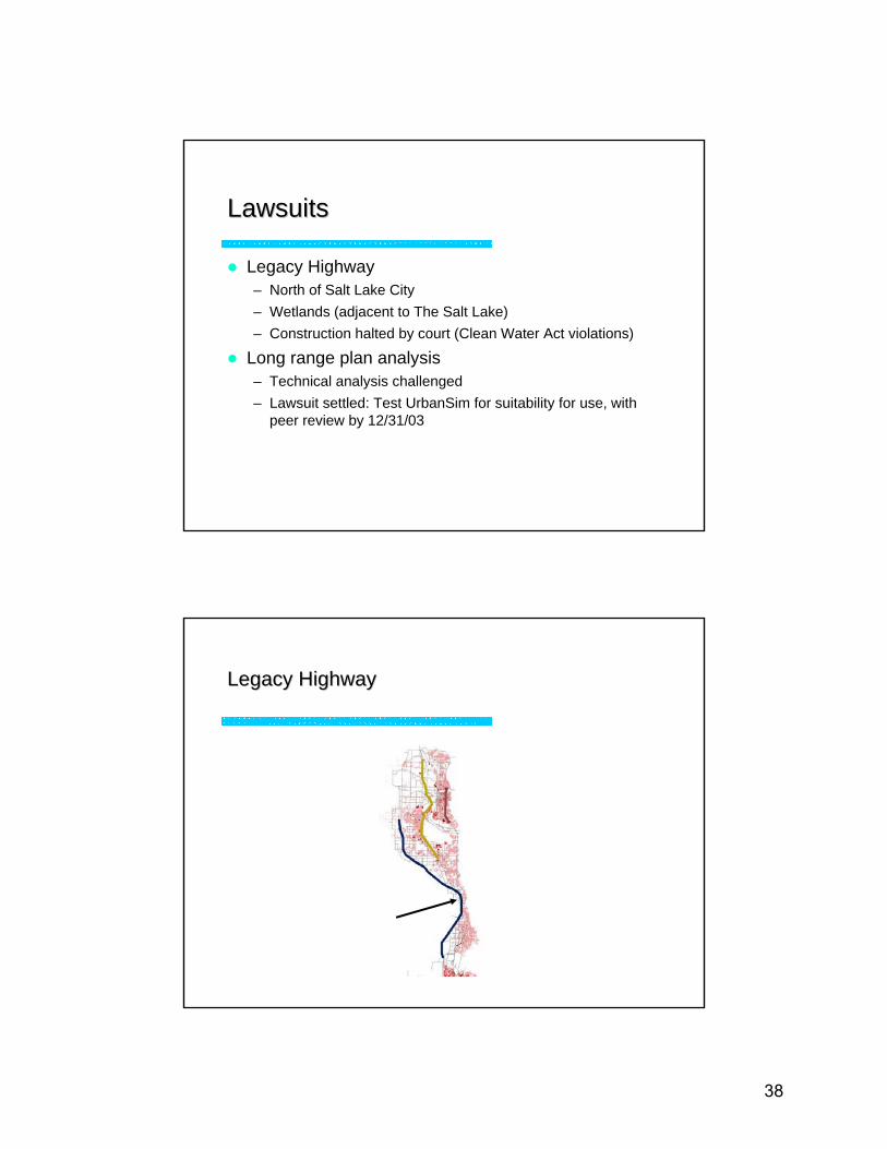
LawsuitsLawsuits
Legacy Highway– North of Salt Lake City– Wetlands (adjacent to The Salt Lake)– Construction halted by court (Clean Water Act violations)
Long range plan analysis– Technical analysis challenged– Lawsuit settled: Test UrbanSim for suitability for use, with
peer review by 12/31/03
Legacy HighwayLegacy Highway
38
WFRC Goals (short to longWFRC Goals (short to long--term)term)
Successful implementation & evaluation of land use model (UrbanSim)Incorporate into MPO modeling workDevelop advanced-practice transportation modelsUse in a visioning process – evaluate scenarios in terms of regional goals
Sensitivity Testing of Integrated Land Sensitivity Testing of Integrated Land Use and Transportation ModelsUse and Transportation Models
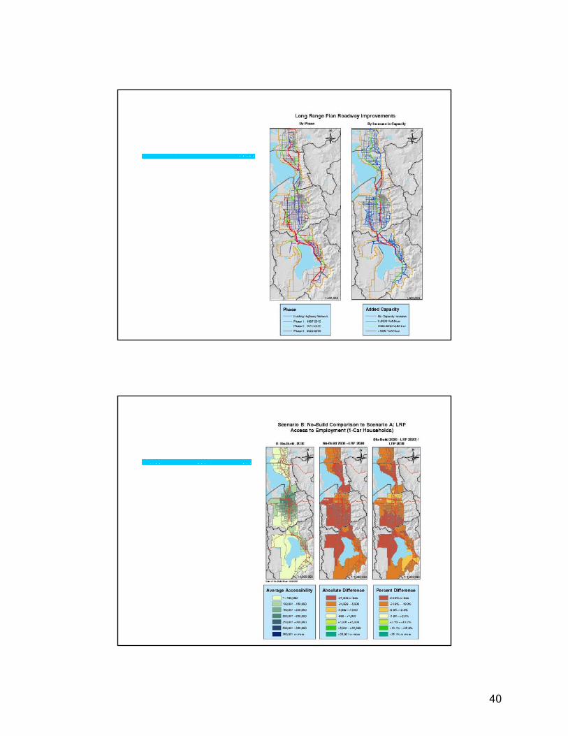
Tested several scenarios:– Long Range Plan (Baseline)– No-build– Drop a highway project– Drop a light rail project– Add parking pricing– Impose Urban Growth Boundary
39
40
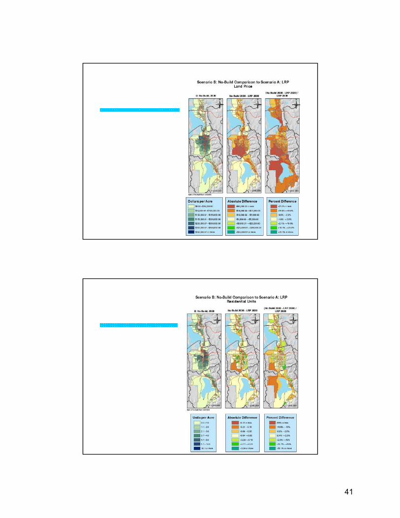
41
Regional Development, Population Trend, and Technology Change Impacts on Future Air
Pollution Emissions in the San Joaquin Valley
Michael KleemanDeb NiemeierSusan Handy
Jay LundWith Song Bai, Sangho Choo, Shengyi Gao, and Julie Ogilvie
University of California Davis
Dana Coe Sullivan Sonoma Technology, Inc.
RD-83184201
Project Objectives
• Develop a system of models for evaluating the impact of local and regional policies and trends on air quality– Global variables from sources like IPCC,
California Department of Finance• Apply this system to the San Joaquin
Valley to evaluate the sensitivity of air quality to different policy scenarios.
42
43
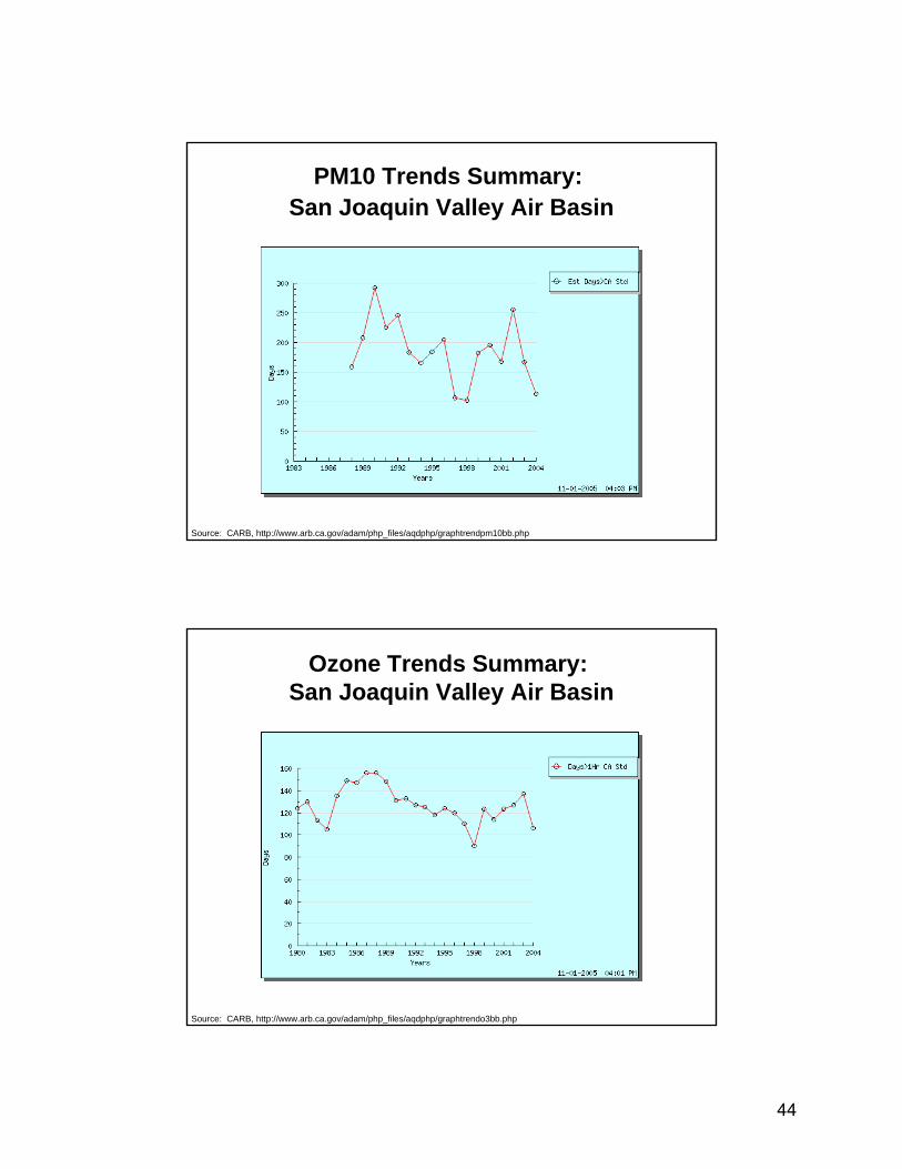
PM10 Trends Summary:San Joaquin Valley Air Basin
Source: CARB, http://www.arb.ca.gov/adam/php_files/aqdphp/graphtrendpm10bb.php
Ozone Trends Summary:San Joaquin Valley Air Basin
Source: CARB, http://www.arb.ca.gov/adam/php_files/aqdphp/graphtrendo3bb.php
44
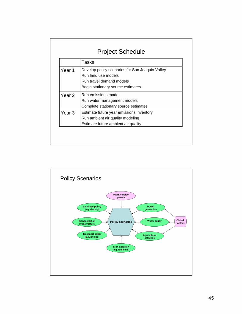
Project Schedule
Estimate future year emissions inventoryRun ambient air quality modelingEstimate future ambient air quality
Year 3
Run emissions modelRun water management modelsComplete stationary source estimates
Year 2
Develop policy scenarios for San Joaquin ValleyRun land use modelsRun travel demand modelsBegin stationary source estimates
Year 1
Tasks
Policy Scenarios
Policy scenarios
Transport policy (e.g. pricing)
Tech adoption (e.g. fuel cells)
Pop& employ growth
Water policy
Agricultural activities
Power generation
Transportation infrastructure
Land-use policy (e.g. density)
Global factors
45
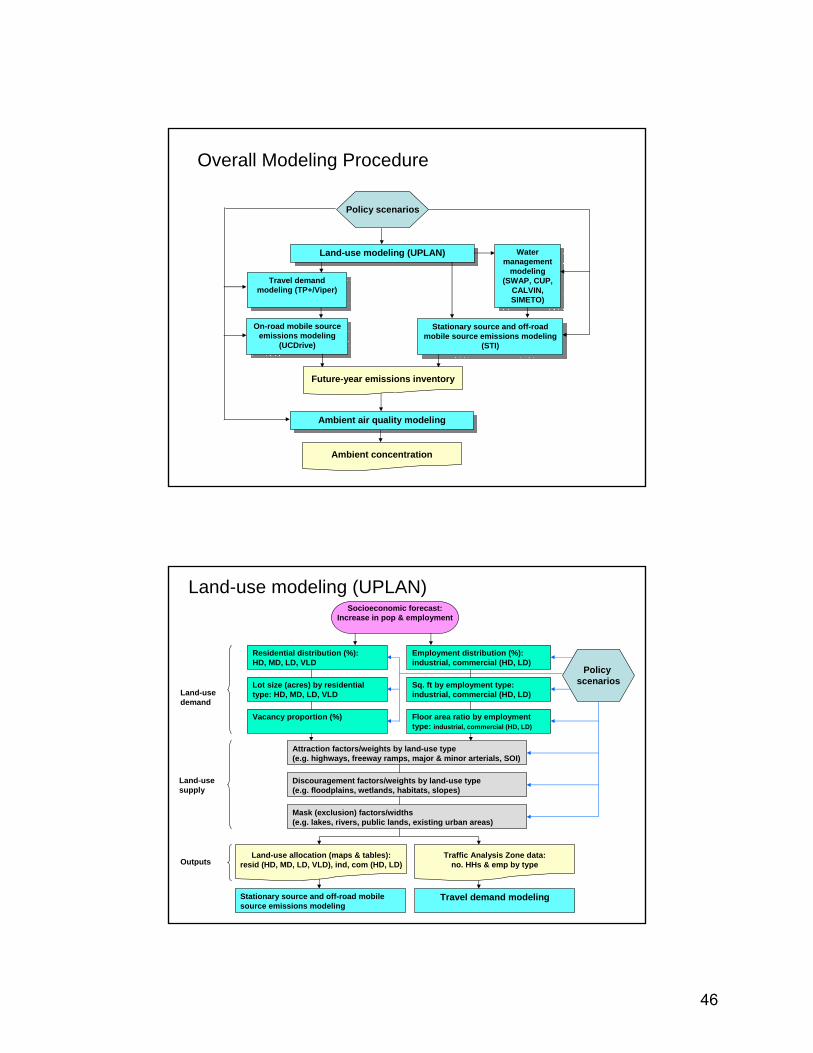
Overall Modeling Procedure
Land-use modeling (UPLAN)Land-use modeling (UPLAN)
Travel demand modeling (TP+/Viper)
Travel demand modeling (TP+/Viper)
Stationary source and off-road mobile source emissions modeling
(STI)
Stationary source and off-road mobile source emissions modeling
(STI)
On-road mobile source emissions modeling
(UCDrive)
On-road mobile source emissions modeling
(UCDrive)
Future-year emissions inventory
Policy scenarios
Ambient air quality modelingAmbient air quality modeling
Ambient concentration
Water management
modeling(SWAP, CUP,
CALVIN, SIMETO)
Water management
modeling(SWAP, CUP,
CALVIN, SIMETO)
Land-use modeling (UPLAN)
Residential distribution (%):HD, MD, LD, VLD
Lot size (acres) by residential type: HD, MD, LD, VLD
Vacancy proportion (%)
Employment distribution (%):industrial, commercial (HD, LD)
Sq. ft by employment type:industrial, commercial (HD, LD)
Floor area ratio by employment type: industrial, commercial (HD, LD)
Socioeconomic forecast:Increase in pop & employment
Attraction factors/weights by land-use type(e.g. highways, freeway ramps, major & minor arterials, SOI)
Discouragement factors/weights by land-use type(e.g. floodplains, wetlands, habitats, slopes)
Mask (exclusion) factors/widths(e.g. lakes, rivers, public lands, existing urban areas)
Land-use demand
Land-use supply
Policy scenarios
Outputs
Travel demand modeling
Land-use allocation (maps & tables):resid (HD, MD, LD, VLD), ind, com (HD, LD)
Traffic Analysis Zone data:no. HHs & emp by type
Stationary source and off-road mobile source emissions modeling
46
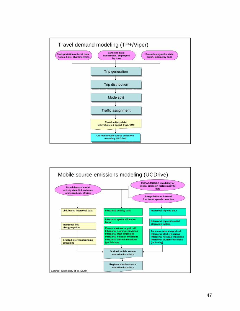
Travel demand modeling (TP+/Viper)
Trip generationTrip generation
Trip distributionTrip distribution
Mode splitMode split
Traffic assignmentTraffic assignment
Land use data: households, employees
by zone
Transportation network data: nodes, links, characteristics
Socio-demographic data:autos, income by zone
Travel activity data:link volumes & speed, trips, VMT
On-road mobile source emissions modeling (UCDrive)
On-road mobile source emissions modeling (UCDrive)
Travel demand model activity data: link volumes
and speed, no. of trips
EMFAC/MOBILE regulatory or modal emission factors activity
data
Interpolation or internal functional speed correction
Link-based interzonal data Intrazonal activity data Interzonal trip-end data
Interzonal link disaggregation
Intrazonal spatial allocation factor Interzonal trip-end spatial
allocation factors
Gridded interzonal running emissions
Zone emissions to grid cell:Intrazonal running emissionsIntrazonal start emissionsIntrazonal hotsoak emissionsIntrazonal diurnal emissions(partial-day)
Zone emissions to grid cell:Interzonal start emissionsInterzonal hotsoak emissionsInterzonal diurnal emissions(multi-day)
Mobile source emissions modeling (UCDrive)
Source: Niemeier, et al. (2004)
Gridded mobile source emission inventory
Regional mobile source emission inventory
47
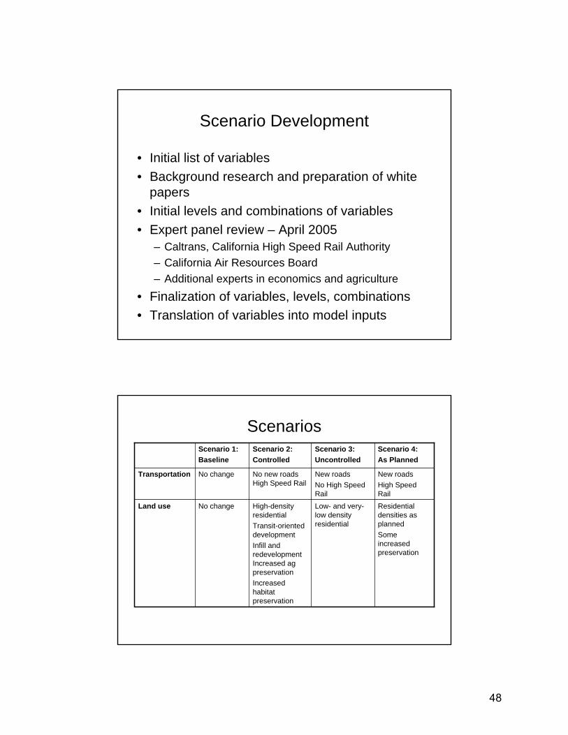
Scenario Development
• Initial list of variables• Background research and preparation of white
papers• Initial levels and combinations of variables• Expert panel review – April 2005
– Caltrans, California High Speed Rail Authority– California Air Resources Board– Additional experts in economics and agriculture
• Finalization of variables, levels, combinations• Translation of variables into model inputs
ScenariosScenario 4:As Planned
Scenario 3:Uncontrolled
Scenario 2:Controlled
Scenario 1:Baseline
No change
No change
High-density residential Transit-oriented developmentInfill and redevelopment Increased agpreservationIncreased habitat preservation
No new roads High Speed Rail
Low- and very-low density residential
New roads No High Speed Rail
Residential densities as plannedSome increased preservation
Land use
New roadsHigh Speed Rail
Transportation
48
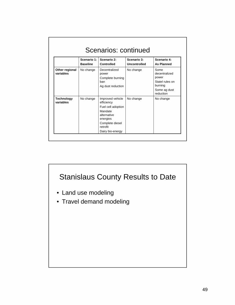
Scenarios: continuedScenario 4:As Planned
Scenario 3:Uncontrolled
Scenario 2:Controlled
Scenario 1:Baseline
No change
No change
Improved vehicle efficiencyFuel cell adoptionMandate alternative energiesComplete diesel retrofitDairy bio-energy
Decentralized power Complete burning banAg dust reduction
No change
No change
No changeTechnology variables
Some decentralized powerStatel rules on burningSome ag dust reduction
Other regional variables
Stanislaus County Results to Date
• Land use modeling• Travel demand modeling
49
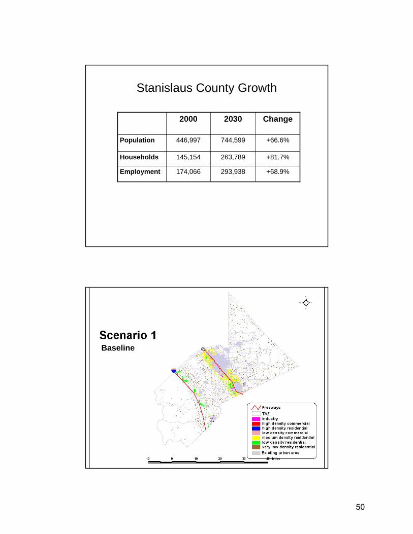
Stanislaus County Growth
293,938
263,789
744,599
2030 Change2000
174,066
145,154
446,997
+68.9%
+81.7%
+66.6%
Employment
Households
Population
Baseline
50
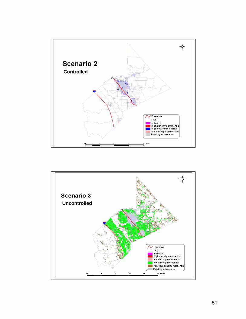
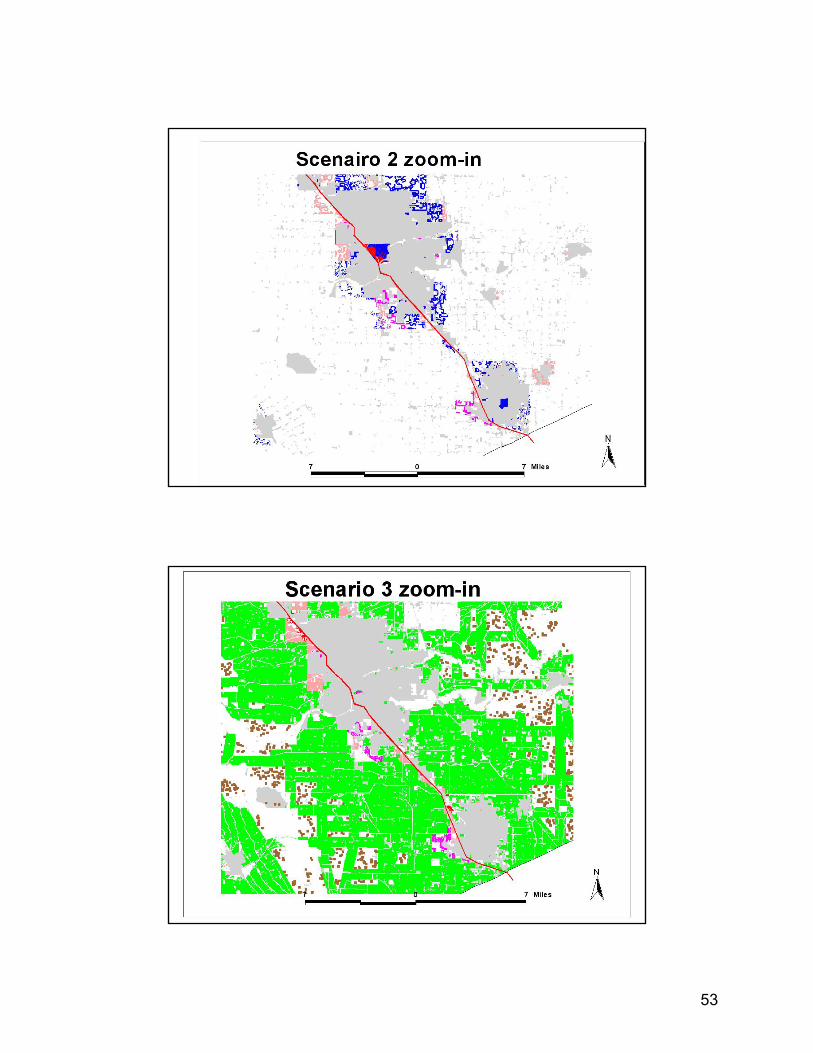
Controlled
Uncontrolled
51
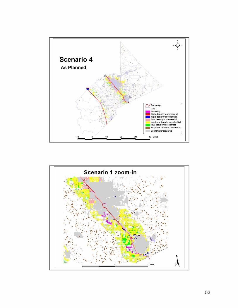
As Planned
52
53
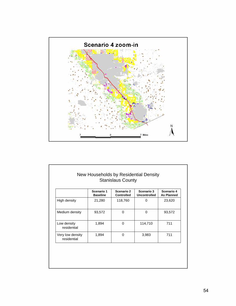
New Households by Residential Density Stanislaus County
7113,98301,894Very low density residential
711114,71001,894Low density residential
93,5720093,572Medium density
23,6200118,76021,280High density
Scenario 4As Planned
Scenario 3Uncontrolled
Scenario 2Controlled
Scenario 1Baseline
54
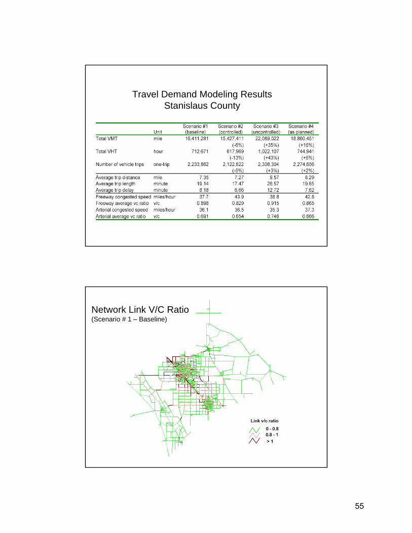
Travel Demand Modeling ResultsStanislaus County
Network Link V/C Ratio(Scenario # 1 – Baseline)
55
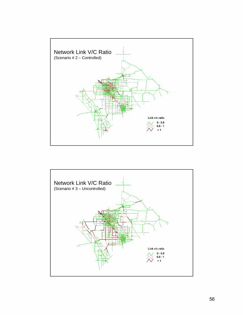
Network Link V/C Ratio(Scenario # 2 – Controlled)
Network Link V/C Ratio(Scenario # 3 – Uncontrolled)
56
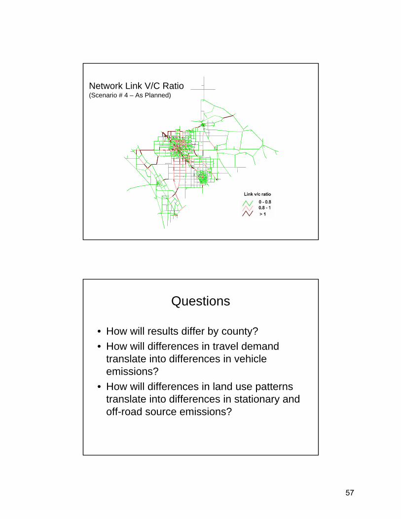
Network Link V/C Ratio(Scenario # 4 – As Planned)
Questions
• How will results differ by county?• How will differences in travel demand
translate into differences in vehicle emissions?
• How will differences in land use patterns translate into differences in stationary and off-road source emissions?
57

Acknowledgements
• United States Environmental Protection Agency Science to Achieve Results (STAR) Grant # RD-83184201
58
Summary of the Q&A Discussion Following Session III
Maurice Abrams, (a “concerned citizen”) Mr. Abrams asked about the status of the Hacienda Project—whether it has been completed. Steve Raney, (Cities21) Mr. Raney replied that the 24-month study was just getting underway. He added, “One of the key things in this study is that the General Manager of the office park, James Paxson, is just a great, progressive guy, and he participates in a lot of forward-thinking transportation studies. He also has a very high social IQ—he’s really well liked—and that was really important as he helped in putting together the letters of support that created the winning grant proposal.” Dr. Raney went on to say that the researchers are “tied in with MTC and BART and the Congestion Management Agency and lots of other good groups, so it’s a pretty exciting team that came together mostly because of James’s unique personality.” ________________________ Steve Raney, (Cities21) Directing his question to Dr. Paul Waddell, Mr. Raney asked, “What’s the order of magnitude of effort to bring the Urban SIM model to the Bay Area or any big place?—Is it four person years of work or what?” Dr. Paul Waddell, (University of Washington) Saying, “You would end with a hard question,” Dr. Waddell stated that as of a year ago the answer would have been “very high” due to the fact that the model is extremely “data hungry, requiring the use of parcel data and business establishment data as well as a lot of data cleaning and data synthesizing.” He acknowledged that that’s where most of the effort has gone. He added, however, that they’ve “been working quite hard over the course of this past year to develop capacity to create much simpler models, so that if one wanted to, you could start with a simpler version and then make it more sophisticated or more sensitive or more detailed, as time and data permit.” Dr. Waddell revealed that in about a month [approximately mid-December 2005] they’re preparing to release a new version that will have the capacity to generate much more quickly “runnable models with local data, but with lighter data requirements and easier construction.” He projected that a “light-weight version of the model could be up and running within 3 to 6 months.” He added that a full-detailed model operating with parcel-level data “really depends on the quality of the data in hand and how long it takes to get it into usable shape.” ________________________ Nancy Levin, (U.S. EPA Region 9) Saying that she works on the environmental review of transportation projects, Ms. Levin stated that one of the questions they deal with is: To what extent does transportation
59
affect land use? She asked the panelists what the current thinking is on that and “whether there is an increasing willingness to use land-use models in looking at impacts of transportation projects.” Dr. Paul Waddell, (University of Washington) Stating that there seemed to be “a couple of questions in there,” Dr. Waddell identified one of them as “How much does transportation influence land use?” Another, he said, pertains to connecting land-use models and the interest in using them. Addressing the first question, Dr. Waddell said, “California has some of the few critics of the argument that transportation influences land use. He specifically named Genevieve Giuliano (USC School of Planning, Policy, and Development), Harry Richardson, and Peter Gordon (both also at USC) as people who have made “pretty strong claims that there are reasons to think that transportation just isn’t what it used to be in influencing land use.” One of the reasons for this belief, he stated, is that in larger metropolitan areas we now have very mature systems, so adding a particular highway or transit project is a fairly incremental change. He said an additional argument used to bolster this case is that multi-worker households make it much harder to minimize commuting time. On the other hand, Dr. Waddell feels that “there is still a large body of evidence to the contrary, that even in a large metropolitan area with a mature transport system building a particular project will have at least localized effects and [a number of projects] will add cumulative effects across the metropolitan region. He stated that he has found that “even in a place as utterly dominated as Salt Lake City, both regional accessibility and local, walking-scale accessibility measures turn out to be significant in predicting people’s location choices in the housing market.” Acknowledging that Susan Handy “has done a lot of work on this topic,” Dr. Waddell yielded the floor to her input. Dr. Susan Handy, (University of California at Davis) Dr. Handy commented, “I don’t think I could answer it any better, Paul.” Dr. Paul Waddell Dr. Waddell asked whether the second question posed by Ms. Levin was whether there is a greater willingness now to use land-use models. Nancy Levin Ms. Levin clarified that in speaking with others from transportation agencies she has found a general reluctance to use land-use models due to great costs, great time involvement, and/or great data needs—basically just the huge investment required. She rephrased her question in this fashion: “Can you only use these models really in a big academic setting for a huge project or is there some move to make them a little bit more accessible to policy makers?”
60
Dr. Paul Waddell Saying, “This is perhaps not totally unrelated to the earlier question,” Dr. Waddell said that “there were several discussions along this line at the Transportation Research Board conference at the beginning of the year.” He added that “there was a sense that academics promoting very complex models—activity-based travel models and integrated land-use and transportation models—may tend to oversell them a little bit, and the practitioners out there who need to implement the models are cautious or skeptical. Essentially, they’re being asked to make huge commitments of time and resources to implement models without a whole lot of evidence to date they’ll make significant differences in what the benefit/cost ratio really is.” Dr. Waddell feels that the skepticism among practitioners is well founded and that academics need to do two things: First, make models easier to implement. Second, “provide more of an incremental development path so that one could start with a simple model, get it running quickly, identify what the weaknesses are in that, and then work on making improvements gradually and with lower levels of investment.” He concluded by saying that it’s important to be able, at each stage, to document what’s been gained and what it cost so that it’s easier to make a case for further development of the project. “Otherwise, it will be rather irrelevant if we can’t make it [i.e., a model] accessible to practitioners.” Dr. Susan Handy Dr. Handy added, “The Transportation Research Board is organizing a conference that will be held in May or June in Austin, Texas that will deal with this very issue: How do you bring all these innovations that are coming out of academia into practice?—sort of helping to build that bridge.” Unidentified Questioner Addressing Dr. Paul Waddell, the questioner said, “Given the effort that is involved in assembling the data for these types of models, is it really the case that what you really need is to assemble the data for the major metropolitan areas and then you can use whatever model is appropriate to use with that? What fraction of the effort involved in setting up a more realistic picture of how transportation interacts with land use is data assembly and data cleaning versus the model itself, and should we perhaps just put that effort into getting the data because we’ll need it for whatever we decide to do?” Dr. Paul Waddell Dr. Waddell commented that “this is an excellent point,” and he said he “would wager that something on the order of 75 percent or so of the effort is in the data” and he added that “there are some important lessons in all that.” One lesson is for agencies/institutions to view the data as “infrastructure that has lots of other uses besides the modeling applications—it enables them to answer lots of questions that they couldn’t answer otherwise.” Consequently, many agencies/institutions are deciding “to go ahead and make commitments and invest in creating databases and maintaining them because they’ll have lots of secondary applications.”
61
Continuing, Dr. Waddell added, “Secondly, I’d say we probably need to be a lot smarter about how we deal with the data development process.” He noted that in the past he and his colleagues simply assumed that they could “get good quality data and integrate it and resolve errors in it to the point that it was completely internally consistent—and then use it in modeling.” As an example, he cited the accounting of where jobs are and where commercial space is—“there’s an implied square-footage-per-employee ratio that tells you how many jobs you can fit into the quantity of space that is available.” He went on to explain that errors in the data can create some really unreasonable or impossible square-footage per employee values that really distort the modeling. Dr. Waddell feels that a lesson from this is that “we should make the modeling much more robust to data artifacts, data errors.” He also thinks “we should probably be synthesizing data a little bit more than we are now, using statistical data mining tools to explore data patterns and being less concerned about getting every single data point exactly right, so we can cut the cost down on getting usable data at a high level of detail.” ________________________ Michael Gill, (U.S. EPA Region 9) Mr. Gill commented that “we are fairly blessed in the West with a lot of land and fairly blessed in this country with low gas prices,” particularly in comparison to Europe. He asked, “Are we learning any lessons from Europe or other places in this realm of transportation and land use?” Steve Raney Mr. Raney responded that “the grocery bag cart that you showed was the one that I used in the Netherlands to walk from my home to my grocery store.” He added, “It’s a cultural thing there—there it’s good to be cheap, which, incidentally, makes you green.” Dr. Benjamin Hobbs Dr. Hobbs said he believes that we’re making some progress and beginning to “get in the right mindset,” although these changes are coming slowly. In his view, the environmental challenges we’re facing dictate that the changes “need to accelerate significantly.” Dr. Susan Handy Dr. Handy added this comment: “Those of us who care about these things look a lot to Europe and say, “Why can’t we do that here?” She believes that, more and more, we are seeing American versions of European ideas. At the same time, “Europe is also seeing a lot more of what we have happening too,” with Wal-mart and suburbanization. She concluded, “Maybe they need to learn from the mistakes we’ve made, as much as we need to learn from the right things they’ve done.” Dr. Paul Waddell Referring to the post-Katrina spike in gas prices, Dr. Waddell said this might provide “one little bit of evidence we have about how people might react to substantially higher gas prices. The sort of spike we’ve seen in transit ridership, for example, provides a little bit of optimism” that sustained higher gasoline prices might bring on meaningful shifts in
62
people’s behavior. He added, “Before this, we didn’t really know what threshold of fuel prices would start to trigger that,” but this episode has provided “at least some glimmer of evidence that there is some elasticity of demand with respect to fuel prices there.” Dr. Waddell went on to say that he wanted to echo what Susan Handy had said about Europe. He explained that he spent last year on sabbatical in the totally pedestrian environment of central Paris—he had no car and walked everywhere. Shortly afterward he went to a seminar on transportation trends, where he heard about “reports on travel surveys that have been done since 1970 or so in the Isle de France region,” and he said he was horrified by what these reports revealed. The trends in central Paris were fairly stable, with very low auto ownership and very high transit ridership being maintained. However, the story in the suburbs is different, with inter-suburban traffic climbing drastically over the years of the studies, and “there’s nothing that gives any indication that the pattern of development and the pattern of transport in the suburbs is anything like the old core of the city.” Dr. Waddell said he believes this is true not just in Paris but in a lot of European cities. This causes him to wonder whether “they have it all figured out and they’re doing things so much better, or whether they have an accident of history on their side—that their cities were built on a more pedestrian transportation economy, and now the outlying areas are developing more on an auto-oriented basis.” He ended by classifying this possibility as “quite scary.” ________________________ END OF SESSION III Q & A
63