IZA DP No. 1488

Socio-Economic Status, Health Shocks,Life Satisfaction and Mortality: Evidence froman Increasing Mixed Proportional Hazard Model

Paul FrijtersJohn Haisken-DeNewMichael A. Shields

DI

SC

US

SI

ON

PA

PE

R S

ER

IE

S

Forschungsinstitutzur Zukunft der ArbeitInstitute for the Studyof Labor

February 2005

Socio-Economic Status, Health Shocks, Life Satisfaction and Mortality:

Evidence from an Increasing Mixed Proportional Hazard Model

Paul Frijters RSSS, Australian National University

John Haisken-DeNew

RWI Essen and IZA Bonn

Michael A. Shields University of Melbourne and IZA Bonn

Discussion Paper No. 1488 February 2005

IZA

P.O. Box 7240 53072 Bonn

Germany

Phone: +49-228-3894-0 Fax: +49-228-3894-180

Email: iza@iza.org

Any opinions expressed here are those of the author(s) and not those of the institute. Research disseminated by IZA may include views on policy, but the institute itself takes no institutional policy positions. The Institute for the Study of Labor (IZA) in Bonn is a local and virtual international research center and a place of communication between science, politics and business. IZA is an independent nonprofit company supported by Deutsche Post World Net. The center is associated with the University of Bonn and offers a stimulating research environment through its research networks, research support, and visitors and doctoral programs. IZA engages in (i) original and internationally competitive research in all fields of labor economics, (ii) development of policy concepts, and (iii) dissemination of research results and concepts to the interested public. IZA Discussion Papers often represent preliminary work and are circulated to encourage discussion. Citation of such a paper should account for its provisional character. A revised version may be available directly from the author.

IZA Discussion Paper No. 1488 February 2005

ABSTRACT

Socio-Economic Status, Health Shocks, Life Satisfaction and Mortality: Evidence from

an Increasing Mixed Proportional Hazard Model

The socio-economic gradient in health remains a controversial topic in economics and other social sciences. In this paper we develop a new duration model that allows for unobserved persistent individual-specific health shocks and provides new evidence on the roles of socio-economic characteristics in determining length of life using 19-years of high-quality panel data from the German Socio-Economic Panel. We also contribute to the rapidly growing literature on life satisfaction by testing if more satisfied people live longer. Our results clearly confirm the importance of income, education and marriage as important factors in determining longevity. For example, a one-log point increase in real household monthly income leads to a 12% decline in the probability of death. We find a large role for unobserved health shocks, with 5-years of shocks explaining the same amount of the variation in length of life as all the other observed individual and socio-economic characteristics (with the exception of age) combined. Individuals with a high level of life satisfaction when initially interviewed live significantly longer, but this effect is completely due to the fact that less satisfied individuals are typically less healthy. We are also able to confirm the findings of previous studies that self-assessed health status has significant explanatory power in predicting future mortality and is therefore a useful measure of morbidity. Finally, we suggest that the duration model developed in this paper is a useful tool when analyzing a wide-range of single-spell durations where individual-specific shocks are likely to be important. JEL Classification: I1, C23 Keywords: income, education, marriage, life satisfaction, shocks, mortality, duration

analysis Corresponding author: Michael A. Shields Department of Economics University of Melbourne Parkville, Melbourne 6010 Australia Email: mshields@unimelb.edu.au

2

1. Introduction

The relationship between socio-economic characteristics and health, and the causal pathways

underlying such a relationship, continues to be a widely debated topic by economists and other

social scientists (see Adda et al., 2003; Adler et al., 1994; Benzeval and Judge, 2001; Case, 2001;

Ettner, 1996; Smith, 1999; van Doorslaer et al., 1997). As noted by Deaton and Paxson (1998),

“There is a well-documented but poorly understood gradient linking socio-economic status to a

wide range of health outcomes”. Economists have recently contributed to the untangling of the

gradient by using large household panel data sets, exogenous variations in income and/or dynamic

econometric techniques to attempt to more firmly establish if income changes do causally affect

adult morbidity. Importantly, all the evidence so far suggests that any such causal effect is weak

and quantitatively small in magnitude (see, for example, Adams et al., 2003, and Meer et al., 2003,

for US evidence; Contoyannis et al., 2004, for the UK; Frijters et al., 2005, for Germany; and

Lindahl, 2005, for Sweden). This is despite it being reasonable to think that higher income could be

used to ‘buy’ a better lifestyle through greater leisure opportunities and improved nutritional intake,

fewer financial worries, better access to medical services and an improved living environment

through better housing and the ability to move to more prosperous neighbourhoods.

A second strand of the literature has focused on the role of socio-economic characteristics in

determining length of life. Two of the pioneering studies on this topic were the first and second

Whitehall studies of Marmot et al. (1984, 1991), which found that men working in the lowest

grades of the British civil service were observed to have death rates significantly higher than those

in the highest grades. In this paper, we aim to shed further light on this important issue by

developing and estimating a duration model that accounts for individual-specific health shocks,

which we apply to high-quality household panel data. So far the studies that have used such data

have found mixed results. For example, while Gerdtham and Johannesson (2004) found an

important role for income in explaining variations in longevity in Sweden using a Proportional

Hazard (PH) model, Gardner and Oswald (2004) found no such role when estimating a binary

probit model of mortality with lagged income using data from the British Household Panel Survey.

However, both studies confirmed previous findings of a positive relationship between marriage and

longevity, and between education and longevity. A detailed review of the earlier literature can be

found in Gardner and Oswald (2004), but it appears that there is still little consensus about the

quantitative importance of socio-economic characteristics in explaining mortality.

In addition to investigating the roles of income, education and marriage, conditioning on initial

health status and measures of wealth, we provide new evidence on the importance of individual-

3

specific health shocks in determining length of life. We also provide what we believe is a novel

contribution to the rapidly growing literature on life satisfaction and happiness (see Oswald, 1997;

Frey and Stutzer, 2002; Frijters et al., 2004, for reviews), by testing if individuals with higher life

satisfaction live longer independent of their socio-economic status. This question also indirectly

relates to the small recent medical literature that finds that more optimistic people have a better

survival rate following certain chronic illness such as cancer (see, for example, Allison et al.,

2003). However, the evidence on this issue is mixed (see Schofield et al., 2004). We are also able

to contribute to the debate about the usefulness of self-assessed measures of morbidity, by testing

whether or not such measures are strong predictors of future mortality (see Idler and Angel, 1990;

Idler and Benysmini, 1997; van Doorslaer and Gerdtham, 2003).

We address these issues using 19 waves of high-quality panel data on around 26,000

individuals followed in the German Socio-Economic Panel (GSOEP) over the period 1984 to 2002.

Important for our analysis, is the fact that when individuals drop-out of the GSOEP panel,

information is collected on the reason, which allows us to identify around 2,400 individuals who

died in this period. We introduce a new duration model that we call the "Increasing Mixed

Proportional Hazard Model" (IMPH), which allows for unobserved heterogeneity that increases

over time due to unobserved persistent health-related shocks. We argue that the assumptions

underlying the IMPH model are superior to the often used Mixed Proportional Hazard Model

(MPH) in the context of modelling length of life, and find strong evidence that health shocks

explain a large part of the variation in longevity. We also suggest that the IMPH model is a useful

tool for modelling a wide range of single spell duration applications in economics and the social

sciences where individual-specific persistent shocks are likely to be important e.g. duration of

unemployment or duration to bankruptcy.

In Section 2 we describe our data, define the main variables used in the analysis and provide

some preliminary statistics. We introduce our modelling framework in Section 3, and the

corresponding results are discussed in Section 4. Conclusions are drawn in Section 5.

2. Data and Sample Properties

To provide new evidence on the roles of socio-economic characteristics and life satisfaction on the

duration of life we use high-quality data drawn from 19 waves of the German Socio-Economic

Panel (GSOEP) between 1984 and 2002. The GSOEP is a nationally representative household

panel that follows a large sample of adults (living in some 7,000 households) each year since 1984.

In 1990, the year of German reunification, the panel was extended to include residents of the

former East Germany. As with any panel survey, the GSOEP suffers from attrition with individuals

4

dropping out of the panel for a variety of reasons. In order to maintain the nationally representative

nature of the data, each year new individuals enter the panel for the first time. For those individuals

that move home, the GSOEP is very successful in following them up. Importantly, in the context of

this study, information is collected from other household members if an individual has died in the

past year, and if this is not possible, this information is obtained from neighbours or from the

official death register. In this paper, we use the full sample of adults in East and West Germany observed in all the

currently available waves of the GSOEP. This comprises 26,401 individuals age over 15, for which

we have 223,723 observations. The average number of years in the panel is 8.47. The average age

of the sample is 44.5 years, 48.8% of respondents are male, 79.9% reside in West Germany and the

average real monthly pre-tax household income is 3,949DM. Household income has been deflated

by the OECD main economic indicators consumer price index (base year 1995).

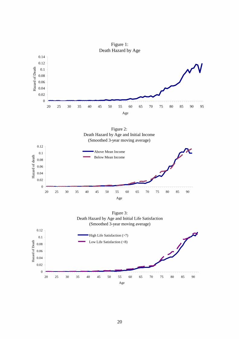
Of the 26,401 individuals we observe, 2,400 died over this period implying a mortality rate of

9.1%. Unfortunately, data is not collected on cause of death. The youngest death we observe is at

age 19 and the oldest death at age 105, with an average age of death of 73 (71 for males, 76 for

females). Figure 1 shows the hazard of death by age. The likelihood of mortality is very small in

Germany up until the age of about 45, then increases gradually between ages 45 and 75, followed

by a steep gradient thereafter. However, the raw data clearly suggests that income plays an

important role in determining survival rates. This is highlighted in Figure 2, where separate hazard

of death by age are shown for individuals with an initially observed real pre-tax monthly household

income above and below the sample mean value. While there is little difference in the death hazard

by income for individuals aged less than 60, individuals initially observed with below mean income

have a higher chance of death between ages 60 and 80. Interestingly, the converse is the case for

those with low incomes who survive until at least 85, although the sample sizes for the most elderly

are small.

Finally, Figure 3 shows the relationship between initially observed life satisfaction and the

hazard of death. Although there appears to be no difference across high and low satisfaction up

until the age of about 74, individuals who report low life satisfaction (i.e. <8 on a 0-10 scale) have a

higher likelihood of death at each age above 74. Therefore there is some evidence from the raw

data that more satisfied individuals live longer.

3. Empirical Models

In this section we outline our empirical strategy by first describing one of the most widely used

5

duration analysis models by economists, namely, the Mixed Proportional Hazard Model (MPH).

We then introduce a new extension to this model, which we have called the “Increasing Mixed

Proportional Hazard Model” (IMPH), and then contrast the underlying assumptions of the two

models. We suggest that the IMPH model is a useful new tool for modelling a wide-range of single-

spell durations in economics when cumulative individual unobserved shocks are likely to be

important and/or when the researcher observes a lot of information about respondents in the initial

interview but little thereafter.

(i) The MPH Model

In the literature on single-spell duration hazard models to date, the Proportional Hazard (PH)

model, and its extension to allow for unobservable heterogeneity, the Mixed Proportional Hazard

(MPH) model, have been by far the most popular. The MPH takes the form:

( | ) '( ) ( )t x z t xθ λ λ φ, = (0.1)

where x is a set of observable characteristics, θ is the hazard rate at duration t, '( )z t is a

continuous baseline function, and 0λ > is a fixed unobservable characteristic. Van den Berg

(2001) provides an extensive survey of the various applications of this model, for which the

durations under scrutiny not only include the length of life, but also include the length of

unemployment, the length of business solvency, the length of wars, the length of time until first

child and the length of time until a stock market crash. This model is identified under a certain set

of assumptions, including the assumptions that λ and x are independent and that ( )E λ is finite

(see Elbers and Ridder, 1982; Heckman and Singer, 1984; Ridder, 1990; and Heckman, 1991).

Various recent extensions deal with the cases where there are multiple durations (Honoré, 1993;

Frijters, 2002), and a combination of multiple and competing durations (Abbring and Van den

Berg, 2003). However, the basic building block of any individual hazard remains the same i.e.

multiplicativity in the various components of the hazard and some observed characteristics (time

varying or not) that are not related toλ .

The treatment of unobservables in this model is unusual for a time-series model. The MPH

model essentially includes the presence of three unobservable components. The first unobservable

component is the fixed individual one (λ ). The second component stems from the fact that even

conditional on observables and λ, the model does not specify an observed event, but only a hazard

6

rate of an event occurring which implicitly means that other time-varying unobservables (whose

distribution is constant) determine whether a transition is made or not. One can call these

‘incidence unobservables’. The third and more hidden unobservable component is the baseline

function '( )z t : duration itself is not a directly meaningful variable and merely proxies for other

time-varying variables. When researchers discuss the hazard to first-time unemployment for

instance, the baseline function is sometimes interpreted as picking up discouragement, stigma and

time-varying benefit entitlements (see Van den Berg, 2001). When researchers discuss the hazard

to death, where the baseline depends on age, the baseline function is interpreted as picking up

health deterioration. The baseline function should therefore more properly be understood as a

common time-varying unobservable.

However, having only common time-varying unobservables is clearly implausible in most

practical applications in economics. In time-series analyses it is normal to have cumulative

unobserved shocks over time. In the case of wage changes for instance, an unobserved promotion

leading to a wage increase is not usually reversed the next period, but is a permanent wage change.

In the case of first-time unemployment also, some time-varying unobservables (such as benefit

entitlements or motivation) are subject to individual-specific persistent shocks. In the case of the

hazard to death, unobserved time-varying cumulative health deterioration occurs but is not the same

for all individuals. We thus argue that it is more natural to assume that time-varying unobservables

have a distribution over the population and are cumulative, leading to an individual-specific path in

the time-varying unobservables rather than a common path.

(ii) The Increasing Mixed Proportional Hazard Model (IMPH)

The main limitation of the MPH model in the context of modelling longevity is that it places an

unduly large emphasis on unobserved health differences at some starting point, whilst paying no

attention to the potentially much greater issue of unobserved cumulative individual health

deteriorations.

We therefore propose the following model to deal with this limitation:

2

( ) '( ) ( )

(0 )

tt

t

t x e z t x

N t

λθ λ φ

λ σ

| , =

,∼ (0.2)

which has both common time-varying unobservables (in '( )z t ) and an individual time-varying

unobservable, tλ . This unobservable is defined to have expectation 0 over the whole population

7

(surviving and not-surviving) at any time, and follows a Wiener process, also known as a random

walk or a unit root process. It can be understood as the accumulation of smaller iid shocks over

time and captures the permanent health shocks that are such a pervasive aspect of real life.1

However, the problem of identification arises in this model because individuals, who are hit by

particularly severe health shocks that increase their hazard rate of dying, are also more likely to

leave the stock of the living over time leaving a selective stock of individuals. Therefore, even

though for the entire population that starts at t=0, E ( ) 0tλ = at any age t, for those that survive until

t, E( ) 0tλ < . We provide a discussion of the conditions needed for identification in the Appendix,

which contains a plausibility argument that the continuous model is (over)identified under weak

assumptions. The discrete version of the model we use in the empirical analysis is also identified.

Importantly, the IMPH model inverts the usual assumption on unobserved heterogeneity:

whilst the MPH assumes there to be heterogeneity at the start of the observation plan which reduces

to zero over time because only those with low unobserved heterogeneity remain in the sample, our

model assumes that there is zero unobserved heterogeneity at the start of the observation plan (i.e.

perfect initial information on hazards) which increases over time due to unobserved persistent

shocks. We take the following parameterisation:

'

1

( )

'( ) a

x

a a

x e

z t e s t s

β

θ

φ

−

=

= ⇐⇒ ≤ < (0.3)

which means β conveys the influence of the observables x; the baseline hazard '( )z t is taken to

be a non-parametric step-function of age where we need to estimate the parameters aθ . We

furthermore take age to be discrete (in years), we have as our information set for each individual i

some individually-specific starting age 0it , a set of characteristics denoted by X which are

observed at some individual-specific calendar time 0iτ , and for the subset that has died before the

end of our observation plan (ending at calendar time S ), we observe age at death iT . The

likelihood of an individual i who still lives at the end of our observation plan (calendar time S ) is

therefore:

1 There are a number of potential extensions and generalizations of this model. One such generalization in a discrete environment is to have an additive process with an unknown distribution of shocks each period. However, in the continuous case any process with unknown additional shocks will closely resemble a Wiener process when aggregated to discrete time intervals.

8

0 01

0

( )0(1 ) ( )

i it a a a

i

t t Ss t s X

t it t

e e e dG Sτ

λ θ β λ τ′

−

= + −∗ ≤ <

=

∑− , −∏∫ (0.4)

where we integrate over the distribution of all paths tλ in the time-interval of length 0iS τ− . It is

also important to bear in mind that t here denotes age and not calendar time. A computational

problem arises when we consider that 0( )t iG Sλ τ, − is in principle of infinite dimension. If we

reduce the dimensionality of tλ to one where there are discrete shocks each year, then

0( )t iG Sλ τ, − is still of dimension 0iS τ− and can thus be extremely large. To solve this, we use a

simulation method whereby we draw a large number M of possible paths tλ from the Wiener

process and integrate over them. Denote each randomly drawn path j as 0 1{ }j j j jTλ λ λ λ= , ,.., where

T denotes the maximum age observed in the sample. Then, our computed likelihood for someone

who remains alive at S equals:

0 0

0 1

0

( ) '

1

1 { (1 )}i i jj

t ti a a a

i

t t SMs t s X

j t t

e e eM

τλ λ θ β−

= + −− ∗ ≤ <

= =

∑−∑ ∏ (0.5)

and the likelihood for someone who is observed to die at age iT equals:

0 1 0 1

0

1( ) ( )' '

1

1 { (1 ) )}i j j jj

t t T ti a a a i i a a i a

i

t TMs t s s T sX X

j t t

e e e e e eM

λ λ λ λθ θβ β− −

= −− −∗ ≤ < ∗ ≤ <

= =

∑ ∑− ∗∑ ∏ (0.6)

where 0 1( ) 'j j

T ti i a a i as T s Xe e eλ λ θ β−− ∗ ≤ <∑ equals the probability of dying at age iT . For large enough M , this

simulated likelihood approaches the true one. The precision of the approximation can further be

increased by reducing the time-interval. Given our data, where individuals are interviewed each

year, the natural unit of time is years. In this application, we have found that taking smaller time

intervals made only a negligible difference to the main parameters of interest. We undertook a

specification search using M=1000, and in a final run used M=2000 and M=5000, neither of which

changed the estimated coefficients noticeably or significantly, implying that M=1000 appears to be

reasonable in practice.

9

(iii) Contrasting the MPH and IMPH Models

The basic idea of the IMPH model versus the MPH model can be clearly illustrated by showing

how the two models work in a hypothetical case. To focus the discussion on the unobserved

heterogeneity distribution, which is the sole item of difference between these two models, consider

a case with no observed heterogeneity and no baseline hazard.

In Figure 4 we have taken a very simple MPH model, where there is only unobserved

heterogeneity which at t=0 follows a uniform distribution on the points {0.01,0.02,..,0.3}. We can

see that at t=0 the unobserved heterogeneity distribution is uniform, but over time the distribution

becomes more and more tilted to the low hazard rates, until after 400 periods, nearly all individuals

surviving in the sample are those with the lowest unobserved hazard rates (i.e. hazards equal to

0.01). This shows a well-known trait of the MPH model, which is that all the ‘high-risks’ (i.e. high

unobserved hazards) sort themselves out of the surviving population, leaving only low-risk

individuals in the surviving population.

Contrast this with the IMPH model. In Figure 5, we take each individual to start with the same

hazard rate in the mid-point of the [0.01,0.3] range, but a Wiener process operates on this

distribution such that at each point in time, the unobserved heterogeneity has an equal chance of

going up as well as down.2 We can see that at t=0, the distribution has a single spike and that as

time passes, the distribution flattens, until finally, after 100 periods, the unobserved heterogeneity

distribution of the survivors follows a bell-type shape. However, the bell is not perfect with the left

tail being thicker than the right tail. This relates to the fact that the mean of the distribution

gradually shifts downwards i.e. it is individuals with shocks that make them less likely to leave that

survive. The survival of the low-risk groups shown in Figures 4 and 5, which results in a shift in the

distribution to the left, is therefore a feature of both the MPH and IMPH models.

One major difference between the MPH and the IMPH models is that the MPH model

presumes to know very little about the population at the start of the sampling frame (t=0), but that

over time one ‘learns’ more and more about the population in the sense that there is less and less

variation in the unobservables and the remaining population is therefore more and more

homogeneous. In contrast, the IMPH presumes to know a lot about the population at the start of the

sampling frame, but ‘loses touch’ with the population in the sense that there is more and more

variation in the unobservables in the surviving population. We argue that for our application the

2 Our specific assumptions here are that the entire population starts at a hazard rate of 0.16, and that every individual at each point in time has a probability of 90% to keep the same hazard rate, a 5% probability of increasing the hazard rate by 0.01, and a 5% probability of decreasing the hazard rate by 0.01 (except at 0.01 itself).

10

latter presumption is more sensible since the GSOEP asks a whole host of question to respondents,

but those who die are often not observed having responded to questions for several years. In fact,

for around 40% of those we observe dying, no questionnaires are responded to in any of the five

years before death. In such a situation, where one knows a lot about a population at some fixed

point in time, but little after that other than who has left the state of interest (in our case, life), we

suggest the IMPH model as the logical model to use rather than the MPH model.

The situation where the researcher observes a great deal of information about a population at

some point in time, but observes far less afterwards, other than whether some particular event took

place, arises often in economics. For example, the unemployed and the disabled are in many data

sets asked many questions at the time that they become unemployed or disabled. However, after

such an ‘intake-interview’, it is often the case that little is known about the respondent other than

whether they leave unemployment or disability. It is very likely that persistent shocks are

unobserved for these people e.g. whether they marry, whether they have followed training, whether

they have moved house and whether they have been active in voluntary work. The IMPH model is

also more appropriate for such situations.

The IMPH model also has other advantages over the MPH model. In particular, the origin of

‘unobserved heterogeneity’ is left unspecified in the MPH model. Unknown factors are presumed

to be present before t=0 which have left permanent differences between individuals. These

unknown factors are often interpreted in labour market context as upbringing or peer influences.

However, once observed in the sample such processes are presumed to have stopped completely i.e.

there is nothing that affects individually-varying unobserved factors once the duration of interest

begins. Upbringing and peer influences essentially ‘stop’. This aspect of the MPH model is often

unappealing. If there are unobserved processes at work creating unobserved differences between

individuals, then it would seem unlikely that these would happen to stop just because individuals

were interviewed or recorded in some other way.

Our model effectively presumes that the outcome of ‘unobserved processes’ are revealed as

specific variables at the start of a sampling period, but that these unobserved processes continue

unabated after that and therefore lead to an increase in unobserved heterogeneity.

A legitimate question is to ask ‘so what’, in the sense of whether there is any good reason to

suppose that the MPH model and the IMPH model are in general going to yield different results.

We show in this study that they do in terms of the quantitative effect of socio-economic

characteristics on mortality. However, the key issue we want to raise in this respect is the

identification of the unobserved heterogeneity distribution in the MPH model applied to single spell

data. As noted by Elbers and Ridder (1982), the unobserved heterogeneity distribution is identified

11

from the change in the relative hazard between a high-risk group and a low-risk group. To illustrate

this, Figure 6 shows a typical profile of the observed relative hazards in a hypothetical environment

(again, without any baseline hazard). In this figure we have supposed that there is a group with an

observed difference whose true effect on the hazard rate is to double it. Both groups start out with

the same unobserved heterogeneity distribution.

The broken line shows the observed relative hazard for the MPH model and the straight line

shows the same statistic for the IMPH model. For the MPH model, the relative hazard of the two

observed groups (high and low) at the start reveals what the true relative effect is. This is an

important observation in the identification of the MPH model, because it is a feature that holds for

all possible MPH models. Over time, however, the relative hazard of the high group first declines

(possibly even below 1) and then returns again to its initial level. This decline is due to sorting,

with those in the high risk group that have high unobserved heterogeneity leaving quickest. This

means that within the high-risk group the unobserved heterogeneity distribution changes faster than

for the low-risk group. In essence, within the high-risk group, those with low unobserved

heterogeneity are very quickly the only individuals remaining, whilst within the low-risk group,

this sorting is much slower. This is the reason why the relative hazard drops even though the true

effect on the hazard of being in the high-risk group remains 2 over the entire period. The observed

relative hazard in the MPH model can even drop below 1, which means that if we do not observe

individuals from the start of the period we could easily draw misleading conclusions.

Consequently, when the start of the spell is not observed for the entire sample, there is an initial-

conditions problem with the MPH model.

For the MPH model this relative hazard profile is not just due to our choice of parameters.

Rather, the general profile holds for all MPH models, regardless of the baseline hazard, the

observed heterogeneity or the unobserved heterogeneity distribution. There is always a dip

followed by a recovery in the relative hazards between the high and low risk groups. However, the

exact shape of the profile is of a particular form: it is unique to a particular unobserved

heterogeneity distribution and hence identifies the unobserved heterogeneity distribution. Such

profiles in empirical practice are therefore used in this way. Baker and Melino (2001) showed that

this source of identification is very weak with finite data and that the MPH model for single spells

is extremely sensitive to the parameterization of the baseline hazards.

The relative hazards in the IMPH model also start out being correct. However, the profile of

the relative hazard is very different to the case of the MPH model. There is still a clear decline in

the relative hazard, but it accelerates over time rather than reduces over time. However, as the

duration goes to infinity, the relative hazard should always tend to 1, since the relative importance

12

of the initial heterogeneity versus the unobserved cumulative shocks becomes less and less.

Therefore, if the IMPH model is correct, the relative hazard of the high risk and the low risk groups

has a very different profile from what the MPH model ‘uses’ to identify parameters and would in

general mean that different parameter estimates can be obtained.

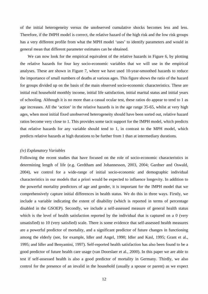
We can now look for the empirical equivalent of the relative hazards in Figure 6, by plotting

the relative hazards for four key socio-economic variables that we will use in the empirical

analyses. These are shown in Figure 7, where we have used 10-year-smoothed hazards to reduce

the importance of small numbers of deaths at various ages. This figure shows the ratio of the hazard

for groups divided up on the basis of the main observed socio-economic characteristics. These are

initial real household monthly income, initial life satisfaction, initial marital status and initial years

of schooling. Although it is no more than a casual ocular test, these ratios do appear to tend to 1 as

age increases. All the ‘action’ in the relative hazards is in the age range 35-65, whilst at very high

ages, when most initial fixed unobserved heterogeneity should have been sorted out, relative hazard

ratios become very close to 1. This provides some tacit support for the IMPH model, which predicts

that relative hazards for any variable should tend to 1, in contrast to the MPH model, which

predicts relative hazards at high durations to be further from 1 than at intermediary durations.

(iv) Explanatory Variables

Following the recent studies that have focused on the role of socio-economic characteristics in

determining length of life (e.g. Gerdtham and Johannesson, 2003, 2004; Gardner and Oswald,

2004), we control for a wide-range of initial socio-economic and demographic individual

characteristics in our models that a priori would be expected to influence longevity. In addition to

the powerful mortality predictors of age and gender, it is important for the IMPH model that we

comprehensively capture initial differences in health status. We do this in three ways. Firstly, we

include a variable indicating the extent of disability (which is reported in terms of percentage

disabled in the GSOEP). Secondly, we include a self-assessed measure of general health status

which is the level of health satisfaction reported by the individual that is captured on a 0 (very

unsatisfied) to 10 (very satisfied) scale. There is some evidence that self-assessed health measures

are a powerful predictor of mortality, and a significant predictor of future changes in functioning

among the elderly (see, for example, Idler and Angel, 1990; Idler and Kasl, 1995; Grant et al.,

1995; and Idler and Benyamini, 1997). Self-reported health satisfaction has also been found to be a

good predictor of future health care usage (van Doorslaer et al., 2000). In this paper we are able to

test if self-assessed health is also a good predictor of mortality in Germany. Thirdly, we also

control for the presence of an invalid in the household (usually a spouse or parent) as we expect

13

that such caring responsibility would be directly detrimental to the health of the carer.

Turning to the economic variables, we control for initial income and wealth, as well as the

prosperity of the region of residence. The income measure we include is the log of real pre-tax total

monthly household income in 1995 prices. We control for wealth in two ways. Firstly, we control

for whether or not the household owns outright or has a mortgage on their home, and conditional on

home ownership, an imputed monthly rentable value of the home. Secondly, we control for the

amount of asset income the household receives per month.

Importantly, we also include controls for marital status, years of schooling and employment

status, all of which we expect, given the results of previous studies, to be significant predictors of

mortality. We also control for number of children in the household and whether or not the

individual was born outside of Germany. In an attempt to contribute to the recent literature that

focused on the potential importance of income inequality on health outcomes (see Gravelle et al.,

2001, for a discussion), following Gerdtham and Johannesson (2004) we include a measure of

average income by geographical area (region in our case) that is time-varying across our 19-year

sample period.

Finally, in order to test whether individuals with high life satisfaction live longer, we control

for initial life satisfaction, which in the GSOEP is reported on the familiar 0 (very unsatisfied) to 10

(very satisfied) scale.

4. Empirical Results

Table 1 presents the parameter estimates from PH models using the entire sample, and then

separately for East and West Germans. The corresponding results from the MPH and IMPH models

using the entire sample are then shown in Table 2.3 The estimates from the PH models are shown in

order to allow for a direct comparison with the results of Gerdtham and Johannesson (2004) for

3 The MPH model we have estimated specifies the mixing distribution to have mass-points. The results presented in Table 2 allow for 2 mass-points, although we have also estimated this model using more mass-points to test for robustness of the main results (see later text). The assumption on mixing is that the mixing occurs at the moment of entering the panel, which is consistent with the assumption that the fixed unobservables are measurement errors in the initial observed characteristics. A natural alternative to ask is whether it would have made sense to estimate a MPH model where the mixing occurs at birth and would thus denote a fixed unobserved health characteristic? The MPH would then, however, be inappropriate as an empirical comparison to the IMPH for this data, mainly because of the initial conditions problem. That is, under the assumptions of the MPH model, the actual sample when mixing occurs at birth is selective because only the ‘good risks’ have survived long enough to make it into the sample. To deal with this, one (explicitly or implicitly) has to make assumptions about the entire life history of all sample participants from birth until entry into the sample. This would entail making detailed assumptions about their marriage, health and employment histories, and all other variables that change over time but are not observed before the start of the sample. Comparing the outcome of such an exercise with the outcomes of the IMPH would be meaningless because of these auxiliary assumptions, which is why we have opted to take the PH as an additional empirical benchmark by which to compare the IMPH model. This is also why we only estimate the MPH under the assumption that the unobservables are measurement errors.

14

Sweden. Moreover, for our purposes the PH model, which does not control for unobserved

heterogeneity, also acts as a useful comparison for the MPH and IMPH models. In this respect, the

PH model is nested in the IMPH model since when the variance of tλ goes to 0, the model reverts

to a PH model. This comparison also leads to a natural test of the validity of the IMPH model,

namely the Likelihood Ratio Test of the additional value of the extra heterogeneity parameter

versus the PH model. The additional Likelihood between the IMPH and the PH model is 91.6 (for

the model using the whole sample), which means the p-value of the IMPH being statistically

‘better’ than the PH is in the order of 0.99999. The significance of the increasing heterogeneity can

also be deduced from the t-value of 12.35 on the log of the standard deviation of tλ .

In contrast, the MPH model is not nested in the IMPH model, and can therefore not be directly

compared by looking at the log likelihood, although we do note that the IMPH has a higher

likelihood. Rather, the fit of the MPH model compared to the IMPH model can be based on the

Akaike information criterion, which equals A(k)=-2*L+2k, where L is the log-likelihood and k is

the number of parameters in the models. The lower the score, the better the model fits the data. We

can see that according to this criterion the IMPH performs statistically best of all three models (the

score of the PH model for the whole sample was 21228.3). As a robustness check on the correct

number of points of support for the MPH model, we re-estimated the MPH model with three points

of support instead of two. This actually led to a lower Akaike information score i.e. the likelihood

with three points of support was -10572.34, which comes at the cost of two extra variables.

(i) Individual-specific health shocks (the IMPH model)

As to the size of the unobserved heterogeneity shocks identified by the IMPH model, the

coefficient on the log of the standard deviation of tλ translates into yearly random shocks that

increase or decrease the hazard rate to death by about 27% (=e-1.3) per standard deviation. This is a

large effect: the difference between the death hazard for an individual aged 40 compared to an 80

year old is about 0.03:1 i.e. an individual aged 80 is per year about 31 times more likely to die than

a similar person aged 40. This is equivalent to about 12.6 standard deviations of the unobserved

shocks, implying that increasing age from 40 to 80 is the same as experiencing 5 or 6 particularly

bad unobserved shocks (slightly above 2 standard deviations). Another way of ascertaining the

importance of the unobserved shocks is to reflect on the fact that the standard deviation of non-age

effects, by which we mean the standard deviation of the total effect of all other observables on the

log-hazard rate, is about 0.592. This is worth 2.2 standard deviations of the unobserved shocks.

Importantly, the unobserved health shocks accumulate to have the same variance as all observed

15

factors within 4.73 years. The IMPH model therefore finds strong support for the existence of large

individual-specific unobserved shocks over time that impact on the hazard of death.

(ii) Socio-economic determinants of mortality

Despite the clear importance of health shocks in the IMPH model, and differences in the

assumptions underlying the three models with regard to unobserved heterogeneity, we find a large

degree of consistency in the parameter estimates of the socio-economic factors affecting mortality

across the PH, MPH and IMPH models.

The findings for the baseline hazard are entirely as expected with the young having a far lower

hazard to death than the old, which we attribute in our modelling framework to unobserved

common deteriorations in health (often captured under the banner of ‘ageing’). Moreover, the

estimates on the socio-economic characteristics to a large extent confirm our prior expectations,

with there being consistent evidence that the death hazard (i.e. the probability of death at any point

in time) significantly increases with being male, being disabled, having an invalid in the household

and being a non-participant in the labour market, and significantly falls with being married, having

more years of schooling, having high initial health satisfaction, having high real household income4

and residing in a more wealthy region of Germany (the latter two effects, however, are not

significant in the PH model for East Germans). In contrast to income, our wealth indictors are not

estimated to be significant predictors of mortality, with the exception of home ownership in East

Germany, which is associated with a lower death hazard. This could be due to the limited nature of

these measures, but if we take them at face value they would imply that accumulated assets simply

‘buy’ little life expectancy. We find no evidence that mortality is affected by number of children.

Contrary to our expectation, being an immigrant in Germany is associated with longer life, but a

higher probability of return migration for immigrants who experience health shocks might be

driving this result.

Turning to the quantitative effects of the main socio-economic variables in explaining

variations in mortality, Table 3 shows the estimated percentage change in the death hazard and the

associated change in expected length of life due to increased household income, being married,

4 The fact that the effect of household income on the death hazard is roughly the same across both East and West Germany, to some extent provides extra credibility to the income finding since, as we have argued in Frijters et al. (2005), incomes in East Germany can be considered mostly driven by exogenous (non-health related) factors in the years following reunification. Moreover, following Gerdtham and Johannesson (2004) we have tested the robustness of the income result to a number of functional forms and income definitions. For example, we have used household equivalent income adjusted for household size and composition. None of these additional tests changed the result of the significant income effect on mortality. These additional results are available on request.

16

having higher health satisfaction and having a great number of years of schooling. Here it is

important to note that a reduction or increase in the death hazard of a certain percentage does not

translate into the same percentage change in expected length of life. This is because a change in the

hazard of death interacts with the baseline hazard. For example, having a 10% lower probability of

dying when an individual is young, and therefore has an extremely low chance of dying anyway, is

going to make very little difference, whereas a 10% higher probability of dying when an individual

is very old, and has a high chance of dying per se, is only going to make a 10% difference within

that age range.

Focusing on the results from the IMPH model, we find that a one-log point increase in real

household monthly income leads to a fall in the death hazard of 12.21% and an increase in expected

length of life of just under one year (at the gravity point). This important role that income has to

play in determining longevity supports the result for Sweden by Gerdtham and Johannesson (2004),

but is in contrast to that found by Gardner and Oswald (2004) who estimated a simple probit model

of mortality using British data. However, while Gerdtham and Johannesson (2004) found no

significant effect of community or area average income on mortality, we find a significantly

positive effect with individual residing in higher income regions, conditional on their own

household income, living longer. From the IMPH estimates, we calculate that residing in a

geographical area with a one-log point higher average income is associated with a 10% decline in

the death hazard, which correspondents to 0.75 years of life. However, the size of this effect is far

higher in the MPH model, accounting for about 5 more years of life. The important role of area

income could be capturing the direct role that income inequality might have on health, or the fact

that richer areas might have better health or public amenities (e.g. such as road safety, less serious

crime). It is certainly an important topic for future research.

Interestingly, the quantitative effect of being married has roughly the same effect as a one-log

point increase in household income, being associated with a 15% reduction in the probability of

death and living 1.17 more years. Self-assessed health, in the form of health satisfaction, is clearly a

good predictor of mortality, with a one point increase on the 0-10 scale leading to a 10% decline in

the death hazard. Moving from 5 to 10 on the scale would therefore be associated with a 50%

decline in the probability of death and 3.75 more years of life. In fact, it is interesting to note that

initial self-assessed health is a stronger predictor of mortality than initial levels of disability. This

also provides some additional support to the validity of using self-assessed health measures as

indicators of morbidity.

An important policy-related question to ask is what is the size of the estimated mortality

differential at the two extremes of the socio-economic characteristics? Holding age, gender and

17

immigrant status constant, we have calculated that an individual who is initially observed in the

panel with the worst possible set of observable socio-economic characteristics is expected to live to

only 43 years of age, in contrast to an individual with high initial health status, no disability, being

married, highly educated, in the top decile of the income distribution and residing in the richest

region etc., who would be expected to live to age 94. If we hold age, gender, immigrant status, and

health satisfaction and disability constant, then the worst possible set of remaining socio-economic

variables would give an expected 59 years of life, and the best set would give 92 years of life.

These results clearly support the argument that socio-economic factors are very important in

explaining variations in length of life across the population.

(iii) The role of life satisfaction

While the parameter estimate on life satisfaction in the IMPH model is negative, suggesting that

individuals who were initially observed in the panel with high life satisfaction have a lower death

hazard, it is not statistically significant. To explore the effect of initial life satisfaction on mortality

further, we re-estimated the model excluding health satisfaction. When we did this the coefficient

on life satisfaction was negative and significant at the 1% level (i.e. -0.041, t-stat = 4.13), with a

one point increase in initial life satisfaction reducing the death hazard by 3.1%. This clearly implies

that more satisfied individuals live longer. However, this is only the case because more satisfied

individuals typically also have a better initial health status. The other parameter estimates were

virtually unchanged.5

We have also tested the robustness of this result by instrumenting life satisfaction using

information on ‘locus of control’ collected in certain years of the GSOEP, which is an assessment

of the extent to which an individual possesses internal or external reinforcement beliefs. It is widely

used as a measure of personality traits by psychologists (see the Journal of Personality and Social

Psychology, for a wide range of articles relating to locus of control and personality traits).

Importantly, this experiment did not change the above life satisfaction result.

5. Conclusions

In this paper we have contributed to the debate about the importance of socio-economic factors in

determining how long individuals live. We have done this in two main ways. Firstly, we have used

19 years of high-quality data on around 26,000 individuals from the German Socio-Economic Panel

Study between 1990 and 2002, of which we observe 2,400 deaths. In this respect our analysis is

5 The full results from these models are available on request.

18

most similar to that undertaken by Gerdtham and Johannesson (2004), who analysed a similar data

set for Sweden. Secondly, as with the Swedish study, we have estimated a number of Proportional

Hazard (PH) models of mortality, but we have also developed a new duration model, which we

have called the Increasing Mix Proportional Hazard Model (IMPH), that explicitly allows for

unobservable individual-specific health shocks. This new model fits the data statistically better than

the other main duration models (the Proportional Hazard Model and the Mixed Proportional Hazard

Model (MPH)), and we find strong evidence that health shocks play a large role in determining

longevity. However, despite the importance of heath shocks the parameter estimates of the various

models in this application are remarkably consistent.

As expected, age, gender and initial health status are strong predictors of death. In addition, we

have found a large role for socio-economic characteristics in determining how long an individual

lives. In particular, we have been able to confirm the positive significant effects of being married

and years of schooling on promoting longevity found for other countries, for both East and West

Germans. With respect to the more contentious issue of the role that income plays in promoting

longevity, we have found that having a higher level of real household income, when initially

observed in the panel, is associated with living significantly longer. Moreover, this effect is

considerably larger than found in the recent literature that has investigated the effect of income on

morbidity using panel data. Specifically, a one-log point increase in household income leads to a

12% reduction in the probability of death. We have also found an important role for average

regional income, with individuals residing in richer regions also living significantly longer. Further

investigation might be able to unravel why this is the case. Importantly, we have calculated,

holding age, gender and immigrant status constant, that an individual with the ‘worst’ socio-

economic characteristics, including poor health and disability, is expected to live to only 43 years

of age, compared to 94 years for an individual with the ‘best’ socio-economic characteristics. If we

also hold health satisfaction and disability constant, then the worst possible set of remaining socio-

economic variables would give an expected 59 years of life, and the best set would give 92 years of

life. Together, we take these findings as strong support for the important role that socio-economic

characteristics play in promoting longevity and explaining mortality variations across the

population.

A new contribution in this paper has been to test whether individuals with high life satisfaction

when initially interviewed in the panel live longer. The raw data and the results for duration models

that do not control for initial self-assessed health status, clearly support this hypothesis.

Importantly, however, once we control for health status this effect is no longer evident capturing

the fact that less satisfied people typically have poorer health. The significant role that self-assessed

19

health has in predicting future mortality confirms previous studies and supports the validity of such

measures of morbidity.

Finally, we believe that the duration estimator that we have developed in this paper is a useful

additional tool for econometricians. It can be applied to a wide-range of single-spell duration

outcomes in economics where unobservable individual-specific persistent shocks are likely to be

important and when little information is observed for individuals after the initial survey interview.

20

Figure 1:Death Hazard by Age

0

0.02

0.04

0.06

0.08

0.1

0.12

0.14

20 25 30 35 40 45 50 55 60 65 70 75 80 85 90 95

Age

Haz

ard

of D

eath

Figure 2:Death Hazard by Age and Initial Income

(Smoothed 3-year moving average)

0

0.02

0.04

0.06

0.08

0.1

0.12

20 25 30 35 40 45 50 55 60 65 70 75 80 85 90

Age

Haz

ard

of d

eath

Above Mean IncomeBelow Mean Income

Figure 3:Death Hazard by Age and Initial Life Satisfaction

(Smoothed 3-year moving average)

0

0.02

0.04

0.06

0.08

0.1

0.12

20 25 30 35 40 45 50 55 60 65 70 75 80 85 90

Age

Haz

ard

of D

eath

High Life Satisfaction (>7)

Low Life Satisfaction (<8)

21

Figure 4:The Distribution of Unobserved Heterogeneity over Time in the MPH model

0

0.2

0.4

0.6

0.8

1

1.2

0.01 0.03 0.05 0.07 0.09 0.11 0.13 0.15 0.17 0.19 0.21 0.23 0.25 0.27 0.29

Unobserved Hazards

Prop

ortio

n of

Sur

vivi

ng P

opul

atio

n

t=0: Uniform Distribution

t=5

t=25

t=45

t=100

t=400

22

Figure 5:The Distribution of Unobserved Heterogeneity over Time in the IMPH Model

0

0.2

0.4

0.6

0.8

1

1.2

0.01 0.03 0.05 0.07 0.09 0.11 0.13 0.15 0.17 0.19 0.21 0.23

Unobserved Hazards

Prop

ortio

n of

Sur

vivi

ng P

opul

atio

n

t=0: Single Peak Distribution

t=5

t=25

t=45t=100

t=10

t=70

23

Figure 6:How Relative Hazards for Observed Groups Change in the MPH and the

IMPH model

0

0.5

1

1.5

2

2.5

1 6 11 16 21 26 31 36 41 46 51 56 61 66 71 76 81Duration

Haz

ard

(Hazard of High Group)/(Hazard Low Group)in the MPH model

(Hazard of High Group)/(Hazard Low Group)in the IMPH model

Figure 7:Death Hazard Ratios by Socio-Economic Characteristics and Age

0

0.5

1

1.5

2

2.5

3

33 38 43 48 53 58 63 68 73 78 83 88 93

Age

Dea

th H

azar

d R

atio

Unmarried \ Married

Low education \ High education

Low income \ High income

Low life satisfaction \ High life satisfaction

24

TABLE 1:

Proportional Hazard Model Estimates of Mortality PH

All West East

Coeff. |t|-stat Coeff. |t|-stat Coeff. |t|-stat

Age < 50 -4.121 38.71 -4.173 36.32 -3.717 12.70

49<age<65 -2.511 29.48 -2.575 27.35 -2.103 10.03

64<age<75 -1.601 22.56 -1.581 20.32 -1.702 9.36

74 < age< 85 -0.690 11.62 -0.685 10.65 -0.745 4.71

Male 0.618 12.42 0.610 11.14 0.651 5.16

Married -0.170 3.34 -0.169 3.05 -0.131 0.93

Number of children -0.001 0.03 0.012 0.29 0.001 0.01

Foreign-born -0.708 8.20 -0.716 7.87 0.005 0.02

Years of schooling -0.040 3.37 -0.036 2.79 -0.076 2.41

% Disabled 0.005 6.21 0.005 6.17 0.003 1.20

Health satisfaction -0.091 10.46 -0.083 8.89 -0.145 5.71

Invalid in household 0.170 2.37 0.076 0.95 0.529 3.38

Employed -0.063 0.65 -0.026 0.24 -0.278 1.28

Non-participant 0.194 2.13 0.207 2.00 0.241 1.18

Life satisfaction 0.016 0.52 -0.002 0.07 0.244 1.59

House owner -0.003 0.53 0.054 0.82 -0.437 2.36

House owner * Imputed rent / 1000 0.001 0.04 -0.001 0.47 0.074 1.12

Asset income / 10000 0.031 0.96 0.028 0.86 0.059 0.20

Log household income -0.095 2.16 -0.099 2.11 -0.100 0.76

Log Average area income -0.139 3.25 -0.153 3.41 -0.079 0.64

West Germany -0.073 1.14

Sample in observed years 338717 289077 49640

Number of individuals 25772 20376 5396

Number of deaths 2236 1878 358

Mean Log Likelihood per year -0.031 -0.031 -0.034

Notes: Absolute t-statistic in parentheses. Omitted categories are female, not married, born in Germany, no invalid in household, unemployed, renter, living in West Germany.

25

TABLE 2:

Mixed Proportional Hazard and Increasing Mixed Proportional Hazard Model Estimates of

Mortality MPH IMPH

All All

Coeff. |t|-stat Coeff. |t|-stat

Age < 50 -3.248 37.05 -4.346 34.75

49 <age< 65 -2.671 28.40 -2.777 25.21

64 <age <75 -1.781 21.80 -1.881 18.99

74 < age< 85 -0.867 10.95 -0.899 11.26

Male 0.657 11.97 0.697 12.12

Married -0.177 3.19 -0.164 2.85

Number of children -0.006 0.16 -0.022 0.52

Foreign-born -0.747 8.46 -0.786 8.56

Years of schooling -0.039 3.15 -0.037 2.90

% Disabled 0.005 6.28 0.005 6.40

Health satisfaction -0.105 10.95 -0.105 10.37

Invalid in household 0.260 3.35 0.239 3.04

Employed -0.068 0.70 -0.089 0.87

Non-participant 0.202 2.14 0.241 2.44

Life satisfaction 0.063 1.92 -0.025 0.71

House owner -0.054 0.80 -0.053 0.75

House owner * Imputed rent / 1000 0.004 0.24 0.001 0.49

Asset income / 10000 0.035 1.05 0.037 1.06

Log household income -0.121 2.45 -0.130 2.51

Log average area income -0.546 2.01 -0.105 2.10

West Germany -0.065 0.66 -0.075 1.07

Log Standard Deviation of Lambda - -1.301 12.35

First point of support 1 - -

Second point of support 42.45 1.79 -

Probability of first point 0.128 - -

Probability of second point 0.872 5.95 -

Sample in observed years 338717 338717

Number of individuals 25772 25772

Number of deaths 2236 2236

Total likelihood -10573.1 -10501.5 Akaike information criterion 21192.18 21047.05

Notes: Absolute t-statistic in parentheses. Omitted categories are female, not married, born in Germany, no invalid in household, unemployed, renter, living in West Germany.

26

TABLE 3:

Estimated Effects of Socio-Economic Characteristics of Mortality PH MPH IMPH

% Change in death hazard

Income 9.08 11.38 12.21

Marriage 15.64 16.25 15.14

Health satisfaction 8.71 9.98 9.98

Years of schooling 3.94 3.81 3.66

Area average income 12.96 42.06 9.98

Additional years of life

Income 1.00 1.12 0.93

Marriage 1.79 1.64 1.17

Health satisfaction 0.96 0.97 0.75

Years of schooling 0.42 0.36 0.27

Area average income 1.46 5.05 0.75

Total socio-economic variation in years of life

Maximum expected years of life 95.62 96.13 93.61

Minimum expected years of life 44.47 38.53 43.14

Notes: The % change in the death hazard and additional years of life are computed for a one-log point increase in real household monthly income, being married relative to being single, a one-point increase on the 0-10 health satisfaction scale, a one-year increase in years of schooling and a one-log point increase in average area income, respectively (holding all else at the sample means). Total socio-economic variation in years of life shows the maximum expected and minimum expected years of life at the two extremes of the socioeconomic characteristics (calculated at the gravity point of the sample and holding age, gender and immigrant status constant).

27

References

Abbring, J. and van den Berg, G. (2003). The nonparametric identification of treatment effects in

duration models. Econometrica, 71, pp. 1491-1517.

Adams, P., Hurd, M., McFadden, D., Merrill, A. and Ribeiro, T. (2003). Healthy, wealthy, and

wise? Tests for direct causal paths between health and socioeconomic status. Journal of

Econometrics, 112, pp. 3-56.

Adda, J., Chandola, T. and Marmot, M. (2003). Socio-economic status and health: Causality and

pathways. Journal of Econometrics, 112, pp. 57-63.

Adler, N. et al. (1994). Socioeconomic status and health: The challenge of the gradient. American

Psychologist, 49, pp. 15-24.

Allison P., Guichard C. and Fung K. et al. (2003). Dispositional optimism predicts survival status 1

year after diagnosis in head and neck cancer patients. Journal of Clinical Oncology, 21, pp.

543-48.

Baker, M. and Melino, A. (2000). Duration dependence and nonparametric heterogeneity: a Monte

Carlo Study. Journal of Econometrics, 96, 57-393.

Benzeval, M. and Judge, K. (2001). Income and health: The time dimension. Social Science and

Medicine, 52, pp. 1371-90.

Case, A. (2001). Does money protect health status? Evidence from South African pensions. NBER

Working Paper no. 8495. Forthcoming in Perspectives on the Economics of Aging, David Wise

(editor), University of Chicago Press, 2004.

Contoyannis, P., Jones, A. and Rice, N. (2004). The dynamics of health in the British Household

Panel Study. Journal of Applied Econometrics, forthcoming.

Deaton, A. and Paxson, C. (1998). Aging the inequality in income and health. American Economic

Review, 88, pp. 248-253.

Elbers, C., Ridder, G. (1982), `True and Spurious Duration Dependence: The Identifiability of the

Proportional Hazard Model', Review of Economic Studies, 49, pp. 403-09.

Ettner, S. (1996). New evidence on the relationship between income and health. Journal of Health

Economics, 15, pp. 67-85.

Frijters, P. (2002). The non-parametric identification of lagged duration dependence. Economics

Letters, 75, pp.289-292.

Frijters, P., Haisken-DeNew, J. and Shields, M. (2004). Changes in the pattern and determinants of

life satisfaction in East and West Germany following reunification. Journal of Human

Resources, 39, pp. 649-674.

Frijters, P., Haisken-DeNew, J. and Shields, M. (2005). The causal effect of income on health:

28

Evidence from German reunification. Journal of Health Economics, forthcoming.

Gardner, J. and Oswald, A. (2004). How is mortality affected by money, marriage, and stress?

Journal of Health Economics, 23, pp. 1181-1207.

Gerdtham, U. and Johannesson, M. (2004). Absolute income, relative income, income inequality

and mortality. Journal of Human Resources, 39, pp. 234- 53.

Grant, M., Zdzisiaw, H. and Chappell, R. (1995). Self-reported health and survival in the

longitudinal study of aging. Journal of Clinical Epidemiology, 48, pp. 375-387.

Gravelle, H., Wildman, J. and Sutton, M. (2001). Income, income inequality and health: what can

we learn from aggregate data? Social Science and Medicine, 54, pp. 577-589.

Heckman, J. and Singer, B. (1984). A method for minimizing the impact of distributional

assumptions in econometric models for duration data. Econometrica, 52, pp. 271-320.

Heckman, J. (1991). Identifying the hand of the past: distinguishing state dependence from

heterogeneity. American Economic Review, 81, pp. 71-79.

Honoré, B. (1993). Identification results for duration models with multiple spells. Review of

Economic Studies, 60, pp. 241-246.

Idler, E. and Angel, R. (1990). Self-rated health and mortality in the NHANES. I. Epidemiologic

follow-up study. American Journal of Public Health, 80, pp. 446-452.

Idler, E. and Benysmini, Y. (1997). Self-reported health and mortality: A review of twenty-seven

community studies. Journal of Health and Social Behavior, 38, pp. 21-37.

Idler, E. and Kasl, S. (1995). Self-rating of health: Do they also predict change in functional

ability? Journal of Gerontology: Social Sciences, 508, pp. S344-S353.

Lindahl, M. (2005). Estimating the effect of income on health and mortality using lottery prizes as

an exogenous source of variation in income. Journal of Human Resources, forthcoming.

Marmot, M., Shipley, M. and Rose, G. (1984). Inequalities in death – specific explanations of a

general pattern. The Lancet, pp. 1003-1006.

Marmot, M., Davey Smith, G., Stansfeld, S., Patel, C., North, F., Head, J., White, I., Brunner, E.,

Feeney, A. (1991). Health inequalities among British civil servants: The Whitehall II Study.

The Lancet, 337, pp. 1387-1393.

Meer, J., Miller, D. and Rosen, H. (2003). Exploring the health-wealth nexus. Journal of Health

Economics, 22, pp. 713-730.

Ridder, G. (1990). The non-parametric identification of generalised accelerated failure-time

models. Review of Economic Studies, 57, pp. 167-82.

Schofield, P., Ball, D. and Smith, J. et al. (2004). Optimism and survival in lung carcinoma

patients. Cancer, 100, pp. 1276-82.

29

Smith, J. (1999). Healthy bodies and thick wallets: The dual relation between health and economic

status. Journal of Economic Perspectives, 13, pp. 145-66.

Van den Berg. G.J. (2001). Duration models: specification, identification, and multiple durations.

In J. Heckman and E. Leamer (eds.), Handbook of Econometrics, Volume 5, North-Holland,

Amsterdam.

van Doorslaer, E. et al. (1997). Income-related inequalities in health: Some international

comparisons. Journal of Health Economics, 16, pp. 93-112.

Van Doorslaer, E. and Gerdtham, U. (2003) Does inequality in self-assessed health predict

inequality in survival by income? Evidence from Swedish data, Social Science and Medicine,

57, pp. 1621-1629

Weir, D. (1995). Family income, mortality, and fertility on the eve of the demographic transition: A

case study of Rosny-Sous-Bois. Journal of Economic History, 55, pp. 1-26.

Appendix

Take the model defined by:

2

( ) ( ) ( )

(0 )

tt

t

t x e z t x

N t

λθ λ φ

λ σ

′| , =

,∼

we make the following additional assumptions:

Assumption 1: ( )z t dt′ = ∞∫ (no defective distribution).

Assumption 2: 2σ is finite.

Assumption 3: ( )xφ has (at least) two distinct points of support, i.e. 0 0( )xφ φ= and 1 1( )xφ φ= .

We can then trivially choose a normalization, and we take 0 1φ = . Conjecture 1 summarises our

plausibility argument.

Conjecture 1: Under Assumptions 1, 2, and 3, the functions ( )z . and ( )xφ , and the parameter 2σ ,

are non-parametrically identified.

30

Motivation: For the sub-populations defined by 0x and x, we have an observed hazard rate equal

to 00 0( ) ( ) t xt x z t Eeλθ φ |′| = and ( ) ( ) ( ) t xt x z t x Eeλθ φ |′| = . Therefore, ( )xφ is identified by

0

( )( )0( ) lim t xt xtx θ

θφ ||↓= . Then, 0(0) ( 0 )z t xθ′ = = | because 0 1t xEeλ | = at 0t = . Knowing 2σ would then

allow a straightforward calculation of ( )z t′ as the solution to a differential equation involving

t xEeλ | . However, this does not yet use information on the difference between 0x and 1x . intuitively

0t xEeλ | is a monotonic decreasing function of 2σ and ( )xφ with (perhaps) a decreasing second

derivative, which would make the information invertible and therefore uniquely identify 2σ .

Remark 1: Without variation in x, the model is not identified because any 2σ and hence any path

tEeλ can be compensated by ( )z t to leave an equivalent model. Like the standard hazard model

therefore, it is the interaction between x and t that identifies the model.

Remark 2: There is some information that is not yet used in this motivation which is useful in

extending the model. To see this, think of the case where there are only infinite shocks in tλ (i.e. no

memory in )tλ , which have a fixed arrival rate δ . It is then the case that ( )0

0 0( ) ( ) ( )dS t x

dtS t x z t xδ φ

|′

| = +

from which we can see that ( ) ( )0 1

( ) ( )0 1

0 1( ) ( )( )dS t x dS t x

dt dtS t x S t x

x xz t φ φ

| |

| |−′−= . This does not use the constraint that ( ) 0z t′ ≥ and

indeed may violate it if the shocks are not in actuality of the infinite-or-nothing variety , which

means there is surplus information. Intuitively, therefore, there is some extra information on the

shape of the distribution of shocks.

Remark 3: We can write the pdf f [ ( )t y T t z tλ φ′= | > , , ] for t>0. It is known at time t=0. For time

t+ , it can be written as: f[ ( )t y T t z tλ φ′+ = | ≥ + , ]=

2( )21 2

22( )

21 22

( )(1 ( ) )

( )(1 ( ) )

Y yY

t

Y sY

t

e f Y e z t dY

e f Y e z t dYds

σπ σ

σπ σ

φ

φ

−−+∞ ′

−∞

−−+∞ ′

−∞

−

−

∫ .∫ ∫

The numerator

can be simplified as 1 ( ) tz t Ee φλφ |′− . The difficulty now is finding the limit of this when goes to

0, and then to build an expression for tdEedt

λ . If the characteristics of tdEedt

λ allow it to be invertible

and smooth, then this, combined with the initial conditions and the differential equation for ( )z t′ ,

would provide uniqueness.

31

Remark 4: The discrete version of this model is identified. We can think of the discrete version as

having unobserved shocks that take place just at the end of one period and before the beginning of

the next. The relative hazards at t=0 then identify ( )xφ . The hazards at t=1 give as many different

hazards that are monotonic in 2σ and ( )z t′ as there are different point of support for x. Therefore,

we would only need two different points of support for x to identify both 2σ and ( )z t′ at t=1. The

discrete version has a great deal of identifying information that is not used, implying the possibility

of specification tests, and the relaxation of some assumptions.